Macroscale structural complexity analysis of subordinated spatiotemporal random fields

José M. Angulo and María D. Ruiz-Medina
Abstract

Large-scale behavior of a wide class of spatial and spatiotemporal processes is characterized in terms of informational measures. Specifically, subordinated random fields defined by non-linear transformations on the family of homogeneous and isotropic Lancaster-Sarmanov random fields are studied under long-range dependence (LRD) assumptions. In the spatial case, it is shown that Shannon mutual information beween marginal distributions for infinitely increasing distance, which can be properly interpreted as a measure of macroscale structural complexity and diversity, has an asymptotic power decay that directly depends on the underlying LRD parameter, scaled by the subordinating function rank. Sensitivity with respect to distortion induced by the deformation parameter under the generalized form given by divergence-based Rényi mutual information is also analyzed. In the spatiotemporal framework, a spatial infinite-dimensional random field approach is adopted. The study of the large-scale asymptotic behavior is then extended under the proposal of a functional formulation of the Lancaster-Sarmanov random field class, as well as of divergence-based mutual information. Results are illustrated, in the context of geometrical analysis of sample paths, considering some scenarios based on Gaussian and Chi-Square subordinated spatial and spatio-temporal random fields.


Keywords: Lancaster-Sarmanov random field models; subordinated random fields; information measures; spatial functional models; structural complexity

1 Introduction

A growing interest is observed, in the last few decades, on the parametric (Bosq, 2000) and nonparametric (Ferraty and Vieu, 2006) spatiotemporal data analysis based on infinite-dimensional spatial models. Particularly, the field of Functional Data Analysis (FDA) has been nurtured by various disciplines, including probability in abstract spaces (see, e.g., Ledoux and Talagrand, 1991). The most recent contributions are developed in the framework of stochastic partial differential and pseudodifferential equations (see, e.g., Ruiz-Medina, 2022). Particularly in the Gaussian random field context, it is well-known that Gaussian measures in Hilbert spaces and associated infinite-dimensional quadratic forms play a crucial role (see Da Prato and Zabczyk, 2002). The tools developed have recently been exploited in several statistical papers on spatiotemporal modeling under the umbrella of infinite-dimensional inference, based on statistical analysis of infinite-dimensional multivariate data and stochastic processes (see, e.g., Frías et al., 2022; Ruiz-Medina, 2022; Torres-Signes et al., 2021). In particular, the statistical distance based approach constitutes a useful tool in hypothesis testing (see, e.g., Ruiz-Medina, 2022, where an estimation methodology based on a Kullback-Leibler divergence-like loss operator is proposed in the temporal functional spectral domain). This methodology has been also exploited in structural complexity analysis based on sojourn measures of spatiotemporal Gaussian and Gamma-correlated random fields. Indeed, there exists a vast literature in the context of stochastic geometrical analysis of the sample paths of random fields based on these measures (see, e.g., Bulinski et al., 2012; Ivanov and Leonenko, 1989, among others). Special attention has been paid to the asymptotic analysis of long-range dependent random fields (see Leonenko, 1999; Leonenko and Olenko, 2014; Makogin and Spodarev, 2022). Recently, in Leonenko and Ruiz-Medina (2022), new spatiotemporal limit results have been derived to analyze, in particular, the limit distribution of Minkowski functionals, in the context of Gaussian and Chi-Square subordinated spatiotemporal random fields.

The geometrical interpretation of these functionals, which, for instance in 2D, is related to the total area of all hot regions, and the total length of the boundary between hot and cold regions, as well as the Euler-Poincaré characteristic, counting the number of isolated hot regions minus the number of isolated cold regions within the hot regions, has motivated several statistical approaches, adopted, for instance, in the Cosmic Microwave Background (CMB) evolution modeling and data analysis (see, e.g., Marinucci and Peccati, 2011).

The present work continues the above-referred research lines in relation to structural complexity analysis of long-range dependent Gaussian and Chi-Square subordinated spatial and spatiotemporal random fields. Indeed, a more general random field framework is considered, defined from the Lancaster-Sarmanov random field class.

The approach adopted here is based on the quantitative assessment in terms of appropriate information-theoretic measures, a framework which has played a fundamental role, with a very extensive related literature, in the probabilistic and statistical characterization and description of structural aspects inherent to stochastic systems arising in a wide variety of knowledge areas. More precisely, the asymptotic behavior, for infinitely increasing distance, of divergence-based Shannon and Rényi mutual information measures, which are formally and conceptually connected to certain forms of ‘complexity’ and ‘diversity’ (see, for instance, Angulo et al. 2021, and references therein), is derived for this random field class. This behavior is characterized by the long-range dependence (LRD) parameter, that in this context determines the global diversity loss, associated with lower values of such a parameter. The deformation parameter $q\neq 1$ involved in the definition of Rényi mutual information also modulates the power rate of decay of this structural dependence indicator as the distance between the considered spatial location increases. As is well-known, the derived asymptotic analysis results based on Shannon mutual information arise as limiting cases, for $q\to 1$, of the ones obtained based on Rényi mutual information. The spatiotemporal case is analyzed in an infinite-dimensional spatial framework. In particular, related spatiotemporal extensions of the Lancaster-Sarmanov random field class, as well as of divergence-based mutual information measures, are formalized under a functional approach. A simulation study is undertaken showing, in particular, that the same asymptotic orders as in the purely spatial case hold for the infinite-dimensional versions of divergence measures here considered (see, e.g., Angulo and Ruiz-Medina, 2023).

The paper content is structured as follows. Section 2 provides the preliminary elements on the analyzed class of Lancaster-Sarmanov random fields, as well as the introduction of information-complexity measures. The main results derived on the asymptotic macroscale behavior of Shannon and Rényi mutual information measures, involving the bivariate distributions of the Lancaster-Sarmanov subordinated random field class studied, are obtained in Section 3. These aspects are illustrated in terms of some numerical examples in subsection 3.3. The functional approach to the spatiotemporal case based on an infinite-dimensional spatial framework is addressed in Section 4. Final comments, with a reference to open research lines, are given in Section 5.

2 Preliminaries

Let $(\Omega,\mathcal{A},P)$ be the basic complete probability space, and denote by $\mathcal{L}^{2}(\Omega,\mathcal{A},P)$ the Hilbert space of equivalence classes (with respect to $P$) of zero-mean second-order random variables on $(\Omega,\mathcal{A},P)$. Consider $X=\{X(\mathbf{z}),\ \mathbf{z}\in\mathbb{R}^{d}\}$ to be a zero-mean spatial homogeneous and isotropic mean-square continuous second-order random field, with correlation function $\gamma(\|\mathbf{x}-\mathbf{y}\|)=\mbox{Corr}\left(X(\mathbf{x}),X(\mathbf{y})\right)$. Assume that the marginal probability distributions are absolutely continuous, having probability density $p(u)$ with support included in $(a,b)$, $-\infty\leq a<b\leq\infty$. Let now $L^{2}((a,b),p(u)du)$ be the Hilbert space of equivalence classes of measurable real-valued functions on the interval $(a,b)$ which are square-integrable with respect to the measure $\mu(du)=p(u)du$.

2.1 Lancaster-Sarmanov random field class

Assume that there exists a complete orthonormal basis $\{e_{k},\ k\geq 0\}$, with $e_{0}\equiv 1$, of the space $L^{2}((a,b),p(u)du)$ such that

$\displaystyle\frac{\partial^{2}}{\partial u\partial v}P\left[X(\mathbf{x})\leq u,X(\mathbf{y})\leq v\right]=:p(u,v,\|\mathbf{x}-\mathbf{y}\|)$
$\displaystyle=p(u)~{}p(v)~{}\left[1+\sum_{k=1}^{\infty}\gamma^{k}(\|\mathbf{x}-\mathbf{y}\|)~{}e_{k}(u)~{}e_{k}(v)\right],\quad\forall\mathbf{x},\mathbf{y}\in\mathbb{R}^{d}.$ (1)

The family of random fields $X$ satisfying the above conditions is known as the Lancaster-Sarmanov random field class (see, e.g., Lancaster, 1958; Leonenko et al., 2017; Sarmanov, 1963). Gaussian and Gamma-correlated random fields are two important cases within this class, with $\{e_{k},\ k\geq 0\}$ being given by the (normalized) Hermite polynomial system in the Gaussian case (see, for example, Peccati and Taqqu, 2011), and by the Laguerre polynomials in the Gamma-correlated case. An interesting special case of the latter is defined by the Chi-Square random field family.

It is well-known that non-linear transformations of these random fields can be approximated in terms of the above series expansions: For every $g\in L^{2}((a,b),p(u)du)$,

$$g(x)=\sum_{k=0}^{\infty}C_{k}^{g}e_{k}(x),\quad\mbox{with}\quad C_{k}^{g}=\int_{a}^{b}g(u)~{}e_{k}(u)~{}p(u)~{}du,\ k\geq 0.$$ (2)

In particular, $C_{0}^{g}=E_{p}[g(X)]$. The minimum integer $m$ such that $C_{k}=0$ for all $1\leq k\leq m-1$ represents the rank of function $g$ in the orthonormal basis $\{e_{k},\ k\geq 0\}$ of the space $L^{2}((a,b),p(u)du)$; that is,

$$g(x)=C_{0}^{g}+\sum_{k=m}^{\infty}C_{k}^{g}e_{k}(x).$$ (3)

In the cases of Gaussian and Gamma-correlated subordinated random fields we will refer to the Hermite and Laguerre ranks, respectively, of function $g$.

An interesting example is Minkowski functional $M_{0}(\nu;X,D)$ providing the random volume of the set of spatial points within $D$ (usually a bounded subset of $\mathbb{R}^{d}$) where random field $X$ crosses above a given threshold $\nu$. That is, denoting by $\lambda$ the Lebesgue measure on $\mathbb{R}^{d}$,

$$M_{0}(\nu;X,D)=\int_{D}1_{\nu}(X(\mathbf{y}))~{}d\mathbf{y}=\lambda(S_{X,D}(\nu)),$$ (4)

where

$$S_{X,D}(\nu)=\left\{\mathbf{z}\in D:\ X(\mathbf{z})\geq\nu\right\}=\left\{\mathbf{z}\in D:\ g(X(\mathbf{z}))=1\right\},$$ (5)

with $g(x)=1_{\nu}(x)$, the indicator function based on threshold $\nu$.

In the Gaussian standard case, since $p(u)=\frac{1}{\sqrt{2\pi}}\exp(-u^{2}/2)$, equation (2) leads to

$$1_{\nu}(x)=\sum_{k=0}^{\infty}\frac{G_{k}(\nu)}{k!}\mathcal{H}_{k}(x),$$

where $\{\mathcal{H}_{k},\ k\geq 0\}$ denotes the basis of (non-normalized) Hermite polynomials, with

$$G_{k}(\nu)=\left\langle 1_{\nu},\mathcal{H}_{k}\right\rangle_{L^{2}((a,b),p(u)du)}=\frac{1}{\sqrt{2\pi}}\exp(-\nu^{2}/2)\mathcal{H}_{k-1}(\nu),\quad k\geq 1,$$

and $G_{0}(\nu)=\frac{1}{\sqrt{2\pi}}\int_{\nu}^{\infty}\exp(-u^{2}/2)du=1-\Phi(\nu)$ (the value of the decumulative normal distribution at $\nu$). Therefore,

$$M_{0}(\nu;X,D)=\sum_{k=0}^{\infty}\frac{G_{k}(\nu)}{k!}\int_{D}\mathcal{H}_{k}(X(\mathbf{y}))~{}d\mathbf{y}$$

(see Leonenko and Ruiz-Medina, 2022).

The following assumption on the large-scale behaviour of the correlation function $\gamma$ is considered:

Assumption I.

$\displaystyle\gamma(\|\mathbf{x}-\mathbf{y}\|)$ $\displaystyle=$ $\displaystyle\mathcal{O}\left(\|\mathbf{x}-\mathbf{y}\|^{-\varrho}\right),\quad\mbox{as}\enspace\|\mathbf{x}-\mathbf{y}\|\to\infty,\quad\varrho\in(0,d).$ (6)

2.2 Information-complexity measures

Since the seminal paper by Shannon (1948), arisen in the context of communications, Information Theory has extraordinarily grown as a fundamental scientific discipline, with a wide projection in many diverse fields of application. In particular, a variety of information and complexity measures have been proposed and thoroughly studied, with the aim of characterizing the uncertain behaviour inherent to random systems.

Although most concepts have a simpler interpretation in the case of systems with a finite number of states, in this preliminary introduction, and in the sequel, we directly refer to definitions for the continuous case, as is the object of this paper. Accordingly, for a continuous multivariate probability distribution with density function $\{f(\mathbf{x}):\mathbf{x}\in\mathbb{R}^{n}\}$, Shannon entropy (in this continuous case, also called ‘differential entropy’) is defined as

$$H(f):=-\int_{\mathbb{R}^{n}}\ln(f(\mathbf{x}))~{}f(\mathbf{x})~{}d\mathbf{x}=E_{f}[-\ln(f)].$$

As is well known, the infimum and supremum of $H(f)$ are $-\infty$ and $+\infty$, respectively. Shannon entropy satisfies ‘extensivity’, i. e. additivity for independent (sub)systems.

Among various generalizations of Shannon entropy, Rényi entropy (Rényi, 1961), based on a deformation (distortion) parameter, constitutes the most representative one under preservation of extensivity. For a continuous multivariate distribution with probability density function $\{f(\mathbf{x}):\mathbf{x}\in\mathbb{R}^{n}\}$, Rényi entropy of order $q$ is defined as

$$H_{q}(f):=\frac{1}{1-q}\ln\left(\int_{\mathbb{R}^{n}}f^{q}(\mathbf{x})~{}d\mathbf{x}\right)=\frac{1}{1-q}\ln\left(E_{f}[f^{q-1}]\right)\qquad(q\neq 1).$$

As before, the infimum and supremum of $H_{q}(f)$ are $-\infty$ and $+\infty$, respectively. Shannon entropy $H(f)$ is the limiting case of Rényi entropy $H_{q}(f)$ as $q\rightarrow 1$, hence also denoted as $H_{1}(f)$.

In particular, Rényi entropy constitutes the basis for the formal definition of the two-parameter generalized complexity measures proposed by López-Ruiz et al. (2009), given by

$$C_{\alpha,\beta}(f):=e^{H_{\alpha}(f)-H_{\beta}(f)},$$

for $0<\alpha,\beta<\infty$.

Campbell (1968) justified the interpretation of Shannon and Rényi entropies in exponential scale (both in the discrete and continuous cases) as an index of ‘diversity’ or ‘extent’ of a distribution. For the continuous case, the diversity index of order $q$,

$$DI_{q}(f)=e^{H_{q}(f)},$$

then varies between 0 and $+\infty$, and

$$C_{\alpha,\beta}(f)=\frac{DI_{\alpha}(f)}{DI_{\beta}(f)},$$

which leads to the interpretation of this concept of complexity in terms of sensitivity of the diversity index of order $q$ with respect to the deformation parameter; see Angulo et al. (2021).

Beyond the assessment on global uncertainty, divergence measures are defined for comparison of two given probability distributions at state level. As before, we here directly focus on versions for the continuous case. For two density functions $\left\{f(\mathbf{x}):\mathbf{x}\in\mathbf{R}^{n}\right\}$ and $\left\{g(\mathbf{x}):\mathbf{x}\in\mathbf{R}^{n}\right\}$, with $f$ being absolutely continuous with respect to $g$, Kullback and Leibler (1951), following the same conceptual approach leading to the definition of Shannon entropy, introduced the (directed) divergence of $f$ from $g$ as

$\displaystyle KL(f\|g)$ $\displaystyle:=\int_{\mathbb{R}^{d}}f(\mathbf{x})~{}\ln\left(\frac{f(\mathbf{x})}{g(\mathbf{x})}\right)~{}d\mathbf{x}=E_{f}\left[\ln\left(\frac{f}{g}\right)\right],$

which, among other uses, has been widely adopted as a meaningful reference measure for inferential optimization purposes. Correspondingly, a generalization is given by Rényi (1961) divergence of order $q$, defined as, for $q\neq 1,$

$\displaystyle H_{q}(f\|g)$ $\displaystyle:=\frac{1}{q-1}\ln\left(\int_{\mathbb{R}^{d}}f(\mathbf{x})~{}\left(\frac{f(\mathbf{x})}{g(\mathbf{x})}\right)^{q-1}d\mathbf{x}\right)=\frac{1}{q-1}\ln\left(E_{f}\left[\left(\frac{f}{g}\right)^{q-1}\right]\right).$

For $q\rightarrow 1$, $H_{q}(f\|g)$ tends to $KL(f\|g)$ (also denoted as $H_{1}(f\|g)$).

Angulo et al. (2021) proposed a natural formulation of a ‘relative diversity’ index of order $q$ as

$$DI_{q}(f\|g)=e^{H_{q}(f\|g)},$$

meaning the structural departure of $f$ from $g$ in terms of the state-by-state probability contribution to diversity. This also gives a complementary interpretation, in terms of sensitivity with respect to the deformation parameter of Rényi divergence, for the two-parameter generalized relative complexity measure introduced by Romera et al. (2011):

$$C_{\alpha,\beta}(f\|g):=e^{H_{\alpha}(f\|g)-H_{\beta}(f\|g)}=\frac{DI_{\alpha}(f\|g)}{DI_{\beta}(f\|g)},$$

for $0<\alpha,\beta<\infty$.

A further step, aiming at quantifying stochastic dependence between two random vectors, is achieved in terms of mutual information measures. From the point of view of departure from independence, divergence measures constitute, in particular, a direct instrumental approach, comparing the (true) joint distribution to the product of the corresponding marginal distributions (hypothetical case of independence). Thus, in the continuous case, for two random vectors $X\sim f_{X}$ and $Y\sim f_{Y}$, with $(X,Y)\sim f_{XY}$, the Rényi-divergence-based measure of mutual information of order $q$ is defined as

$\displaystyle I_{q}(X,Y)$ $\displaystyle:=H_{q}(f_{XY}\|f_{X}f_{Y}),$ (7)

including the special case

$\displaystyle I(X,Y)$ $\displaystyle:=KL(\bar{p}_{XY}\|\bar{p}_{X}\bar{p}_{Y})=H(X)+H(Y)-H(X,Y)$ (8)

(with the last equality not being similarly satisfied, in general, for $q\neq 1$). Related concepts and interpretations can be derived in relation to ‘mutual complexity’ and ‘mutual diversity’ (see, e. g., Alonso et al., 2016; Angulo et al., 2021).

These elements are applied in the next sections to studying, under the informational approach, the large-scale asymptotic behaviour of real and infinite-dimensional valued (for the spatio-temporal case) random fields of Lancaster-Sarmanov type.

3 Methodology: mutual information dependence assessment

In this section, we apply equation (6) in the derivation of the asymptotic order characterizing the spatial macroscale behaviour of mutual information between the marginal spatial components of Lancaster-Sarmanov subordinated random fields. Under Assumption I, this asymptotic order is related to the LRD parameter $\varrho$ of the underlying Lancaster-Sarmanov random field. Note that the lower values of $\varrho$ correspond to higher asymptotic structural diversity loss. Such an asymptotic order is evaluated in Section 3.1, in particular, for mutual information based on Shannon entropy, which corresponds to a limiting case of the asymptotic spatial macroscale order of mutual information based on Rényi entropy.

3.1 Asymptotic analysis from Shannon mutual information

Let $\{X(\mathbf{x}),\ \mathbf{x}\in\mathbb{R}^{d}\}$ be an element of the Lancaster-Sarmanov random field class. From equation (1), mutual information between component r.v.’s $X(\mathbf{x})$ and $X(\mathbf{y})$ can be computed as follows:

$\displaystyle I(X(\mathbf{x}),X(\mathbf{y}))=\int_{a}^{b}\int_{a}^{b}p(u,v,\|\mathbf{x}-\mathbf{y}\|)~{}\ln\left(\frac{p(u,v,\|\mathbf{x}-\mathbf{y}\|)}{p(u)~{}p(v)}\right)~{}dudv$
$\displaystyle=\int_{a}^{b}\int_{a}^{b}p(u)~{}p(v)~{}\left[1+\sum_{k=1}^{\infty}\gamma^{k}(\|\mathbf{x}-\mathbf{y}\|)~{}e_{k}(u)~{}e_{k}(v)\right]~{}$
$\displaystyle\hskip 28.45274pt\times\ln\left(1+\sum_{k=1}^{\infty}\gamma^{k}(\|\mathbf{x}-\mathbf{y}\|)~{}e_{k}(u)~{}e_{k}(v)\right)~{}dudv.$ (9)

The following lemma shows that, under Assumption I, the asymptotic behavior of $\mathcal{S}_{\varrho}(\|\mathbf{x}-\mathbf{y}\|):=I(X(\mathbf{x}),X(\mathbf{y}))$, when $\|\mathbf{x}-\mathbf{y}\|\to\infty$, involves the LRD parameter $\varrho$, thus providing an indicator of diversity loss at macroscale, with higher values attained as $\varrho$ gets closer to 0.

Lemma 1

Under Assumption I, the following asymptotic behavior holds:

$$\mathcal{S}_{\varrho}(\|\mathbf{x}-\mathbf{y}\|)=\mathcal{O}\left(\|\mathbf{x}-\mathbf{y}\|^{-\varrho}\right),\quad\mbox{as}\enspace\|\mathbf{x}-\mathbf{y}\|\to\infty.$$ (10)

Proof. Note that $p(u)\in L^{2}((a,b),p(u)du)$ admits the series expansion

$$p(u)=\sum_{k=0}^{\infty}C_{k}^{p}e_{k}(u),\quad\mbox{with}\quad C_{k}^{p}=\int_{a}^{b}[p(u)]^{2}~{}e_{k}(u)~{}du,\quad k\geq 0.$$

From equation (9), applying Taylor series expansion of logarithmic function at a neighborhood of 1, keeping in mind that $\sum_{k=0}^{\infty}\left[C_{k}^{p}\right]^{2}<\infty,$ we obtain

$\displaystyle\mathcal{S}_{\varrho}(\|\mathbf{x}-\mathbf{y}\|)=I(X(\mathbf{x}),X(\mathbf{y}))\simeq\int_{a}^{b}\int_{a}^{b}\left[\sum_{k=0}^{\infty}C_{k}^{p}~{}e_{k}(u)\right]\left[\sum_{l=0}^{\infty}C_{l}^{p}~{}e_{l}(v)\right]$
$\displaystyle\times\left[1+\sum_{i=1}^{\infty}\gamma^{i}(\|\mathbf{x}-\mathbf{y}\|)~{}e_{i}(u)~{}e_{i}(v)\right]\left[\sum_{j=1}^{\infty}\gamma^{j}(\|\mathbf{x}-\mathbf{y}\|)~{}e_{j}(u)~{}e_{j}(v)\right]~{}dudv$
$\displaystyle=\sum_{j=1}^{\infty}\gamma^{j}(\|\mathbf{x}-\mathbf{y}\|)\left[C_{j}^{p}\right]^{2}+\sum_{i=1}^{\infty}\sum_{j=1}^{\infty}\gamma^{i+j}(\|\mathbf{x}-\mathbf{y}\|)$
$\displaystyle\hskip 28.45274pt\times\int_{a}^{b}\int_{a}^{b}~{}e_{i}(u)~{}e_{i}(v)~{}e_{j}(u)~{}e_{j}(v)~{}p(u)~{}p(v)~{}dudv$
$\displaystyle=\sum_{j=1}^{\infty}\gamma^{j}(\|\mathbf{x}-\mathbf{y}\|)\left[C_{j}^{p}\right]^{2}+\sum_{i=1}^{\infty}\sum_{j=1}^{\infty}\gamma^{i+j}(\|\mathbf{x}-\mathbf{y}\|)~{}\delta_{i,j}$
$\displaystyle=\ \sum_{j=1}^{\infty}\gamma^{j}(\|\mathbf{x}-\mathbf{y}\|)\left[C_{j}^{p}\right]^{2}+\sum_{i=1}^{\infty}\gamma^{2i}(\|\mathbf{x}-\mathbf{y}\|)$
$\displaystyle\leq$ $\displaystyle\left(\sup_{j\geq 1}\left[C_{j}^{p}\right]^{2}\right)\sum_{j=1}^{\infty}\gamma^{j}(\|\mathbf{x}-\mathbf{y}\|)+\sum_{i=1}^{\infty}\gamma^{2i}(\|\mathbf{x}-\mathbf{y}\|)$
$\displaystyle=\ \left(\sup_{j\geq 1}\left[C_{j}^{p}\right]^{2}\right)\frac{\gamma(\|\mathbf{x}-\mathbf{y}\|)}{1-\gamma(\|\mathbf{x}-\mathbf{y}\|)}+\frac{\gamma^{2}(\|\mathbf{x}-\mathbf{y}\|)}{1-\gamma^{2}(\|\mathbf{x}-\mathbf{y}\|)}$
$\displaystyle=\mathcal{O}\left(\|\mathbf{x}-\mathbf{y}\|^{-\varrho}\right),\quad\mbox{as}\enspace\|\mathbf{x}-\mathbf{y}\|\to\infty.$

Similarly, as $\|\mathbf{x}-\mathbf{y}\|\to\infty,$

$\displaystyle\mathcal{S}_{\varrho}(\|\mathbf{x}-\mathbf{y}\|)$ $\displaystyle=$ $\displaystyle I(X(\mathbf{x}),X(\mathbf{y}))\simeq\sum_{j=1}^{\infty}\gamma^{j}(\|\mathbf{x}-\mathbf{y}\|)\left[C_{j}^{p}\right]^{2}+\sum_{i=1}^{\infty}\gamma^{2i}(\|\mathbf{x}-\mathbf{y}\|)$
$\displaystyle\geq$ $\displaystyle\sum_{j=1}^{\infty}\gamma^{j}(\|\mathbf{x}-\mathbf{y}\|)\left[C_{j}^{p}\right]^{2}$
$\displaystyle\geq$ $\displaystyle\left(\inf_{j\geq 1}\left[C_{j}^{p}\right]^{2}\right)\sum_{j=1}^{\infty}\gamma^{j}(\|\mathbf{x}-\mathbf{y}\|)=\mathcal{O}\left(\|\mathbf{x}-\mathbf{y}\|^{-\varrho}\right),$

where we have applied that the rank of function $p\in L^{2}((a,b),p(u)du)$ is equal to 1.

For $g\in L^{2}((a,b),p(u)du)$, a similar asymptotic behavior is displayed by mutual information $I(g(X(\mathbf{x})),g(X(\mathbf{y})))$ when $\|\mathbf{x}-\mathbf{y}\|\to\infty$, involving the LRD parameter $\varrho$ scaled by the rank $m$ of function $g$ in the orthonormal basis $\{e_{k},\ k\geq 0\}$ (Hermite and Laguerre ranks in the Gaussian and Gamma-correlated cases, respectively). This fact is proved in the following result.

Theorem 1

Let $p(u)$ be, as before, the probability density characterizing the marginal probability distributions of the Lancaster-Sarmanov random field $X=\{X(\mathbf{z}),\ \mathbf{z}\in\mathbb{R}^{d}\}$. Assume that $g\in L^{2}((a,b),p(u)du)$ has rank $m$, and is such that $g(X(\mathbf{z}))$ is a discrete random variable whose state space is finite (with cardinal $N$), for $\mathbf{z}\in\mathbb{R}^{d}.$ The following asymptotic behavior then holds:

$$I\left(g(X(\mathbf{x})),g(X(\mathbf{y}))\right)=\mathcal{O}\left(\|\mathbf{x}-\mathbf{y}\|^{-m\varrho}\right),\quad\mbox{as}\enspace\|\mathbf{x}-\mathbf{y}\|\to\infty.$$ (13)
Remark 1

Note that applying variable change theorem, equation (13) is also satisfied in the case where, for every $\mathbf{z}\in\mathbb{R}^{d},$ $g(X(\mathbf{z}))$ is a continuous random variable and $g$ admits an inverse function $g^{-1}$ having non-null derivatives over $g((a,b)).$ Identity (13) also holds when $g$ is non injective but a countable set $\{g_{k}^{-1}(\mathbf{y}),\ k\in\mathbb{N}\}$ of preimages is associated with every point $\mathbf{y}\in g((a,b)),$ with $g_{k}^{-1}$ having non-null derivatives over $g((a,b)),$ for $k\in\mathbb{N}.$

Proof. Under Assumption I, applying Jensen’s inequality, since $\{e_{k},\ k\geq 0\}$ is an orthonormal basis of the space $L^{2}((a,b),p(u)du),$

$\displaystyle I\left(g(X(\mathbf{x})),g(X(\mathbf{y}))\right)=\sum_{i=1}^{N}\sum_{j=1}^{N}\ln\left[\frac{p_{g(X(\mathbf{x})),g(X(\mathbf{y}))}(g_{i},g_{j})}{p_{g(X(\mathbf{x}))}(g_{i})~{}p_{g(X(\mathbf{y}))}(g_{j})}\right]$
$\displaystyle\times\int_{g^{-1}(g_{i})\times g^{-1}(g_{j})}p(u)~{}p(v)~{}\left[1+\sum_{h=m}^{\infty}\gamma^{h}(\|\mathbf{x}-\mathbf{y}\|)~{}e_{h}(u)~{}e_{h}(v)\right]~{}dudv$
$\displaystyle\leq\sup_{i,j}\left(\ln\left[\frac{p_{g(X(\mathbf{x})),g(X(\mathbf{y}))}(g_{i},g_{j})}{p_{g(X(\mathbf{x}))}(g_{i})~{}p_{g(X(\mathbf{y}))}(g_{j})}\right]\right)$
$\displaystyle\times\enspace N^{2}\left[1+\sum_{h=m}^{\infty}\gamma^{h}(\|\mathbf{x}-\mathbf{y}\|)\int_{a}^{b}\int_{a}^{b}p(u)~{}p(v)~{}e_{h}(u)~{}e_{h}(v)~{}dudv\right]$
$\displaystyle=\sup_{i,j}\left(\ln\left[\frac{p_{g(X(\mathbf{x})),g(X(\mathbf{y}))}(g_{i},g_{j})}{p_{g(X(\mathbf{x}))}(g_{i})~{}p_{g(X(\mathbf{y}))}(g_{j})}\right]\right)$
$\displaystyle\hskip 28.45274pt\times N^{2}\left[1+\sum_{h=m}^{\infty}\gamma^{h}(\|\mathbf{x}-\mathbf{y}\|)\left(E_{p}\left[e_{h}(\cdot)\right]\right)^{2}\right]$
$\displaystyle\leq\sup_{i,j}\left(\ln\left[\frac{p_{g(X(\mathbf{x})),g(X(\mathbf{y}))}(g_{i},g_{j})}{p_{g(X(\mathbf{x}))}(g_{i})~{}p_{g(X(\mathbf{y}))}(g_{j})}\right]\right)$
$\displaystyle\hskip 28.45274pt\times N^{2}\left[1+\sum_{h=m}^{\infty}\gamma^{h}(\|\mathbf{x}-\mathbf{y}\|)\|e_{h}\|_{L^{2}((a,b),p(u)du)}^{2}\right]$
$\displaystyle=\sup_{i,j}\left(\ln\left[\frac{p_{g(X(\mathbf{x})),g(X(\mathbf{y}))}(g_{i},g_{j})}{p_{g(X(\mathbf{x}))}(g_{i})~{}p_{g(X(\mathbf{y}))}(g_{j})}\right]\right)$
$\displaystyle\hskip 28.45274pt\times N^{2}\left[\gamma^{0}(\|\mathbf{x}-\mathbf{y}\|)+\sum_{h=m}^{\infty}\gamma^{h}(\|\mathbf{x}-\mathbf{y}\|)\right]$
$\displaystyle=\mathcal{O}\left(\|\mathbf{x}-\mathbf{y}\|^{-m\varrho}\right),\quad\mbox{as}\enspace\|\mathbf{x}-\mathbf{y}\|\to\infty.$ (14)

From (1), the following lower bound is obtained:

$\displaystyle I\left(g(X(\mathbf{x})),g(X(\mathbf{y}))\right)=\sum_{i=1}^{N}\sum_{j=1}^{N}\ln\left[\frac{p_{g(X(\mathbf{x})),g(X(\mathbf{y}))}(g_{i},g_{j})}{p_{g(X(\mathbf{x}))}(g_{i})~{}p_{g(X(\mathbf{y}))}(g_{j})}\right]$
$\displaystyle\times\int_{g^{-1}(g_{i})\times g^{-1}(g_{j})}p(u)~{}p(v)~{}\left[1+\sum_{h=m}^{\infty}\gamma^{h}(\|\mathbf{x}-\mathbf{y}\|)~{}e_{h}(u)~{}e_{h}(v)\right]~{}dudv$
$\displaystyle\geq\inf_{i,j}\left(\ln\left[\frac{p_{g(X(\mathbf{x})),g(X(\mathbf{y}))}(g_{i},g_{j})}{p_{g(X(\mathbf{x}))}(g_{i})~{}p_{g(X(\mathbf{y}))}(g_{j})}\right]\right)$
$\displaystyle\times\enspace N^{2}\left[1+\left[\sum_{h=m}^{\infty}\gamma^{h}(\|\mathbf{x}-\mathbf{y}\|)\right]\int_{\mathcal{S}\times\mathcal{S}}e_{h}(u)~{}e_{h}(v)~{}p(u)~{}p(v)~{}dudv\right]$
$\displaystyle=\inf_{i,j}\left(\ln\left[\frac{p_{g(X(\mathbf{x})),g(X(\mathbf{y}))}(g_{i},g_{j})}{p_{g(X(\mathbf{x}))}(g_{i})~{}p_{g(X(\mathbf{y}))}(g_{j})}\right]\right)$
$\displaystyle\times\enspace N^{2}\left[\left(E_{p}[1_{\mathcal{S}}e_{h}(\cdot)]\right)^{2}+\left[\sum_{h=m}^{\infty}\gamma^{h}(\|\mathbf{x}-\mathbf{y}\|)\right]\left(E_{p}[1_{\mathcal{S}}e_{h}(\cdot)]\right)^{2}\right]$
$\displaystyle\geq\inf_{i,j}\left(\ln\left[\frac{p_{g(X(\mathbf{x})),g(X(\mathbf{y}))}(g_{i},g_{j})}{p_{g(X(\mathbf{x}))}(g_{i})~{}p_{g(X(\mathbf{y}))}(g_{j})}\right]\right)$
$\displaystyle\times\enspace\left[N\left(\inf_{h\geq m}E_{p}[1_{\mathcal{S}}e_{h}(\cdot)]\right)\right]^{2}\left[\gamma^{0}(\|\mathbf{x}-\mathbf{y}\|)+\sum_{h=m}^{\infty}\gamma^{h}(\|\mathbf{x}-\mathbf{y}\|)\right]$
$\displaystyle=\mathcal{O}\left(\|\mathbf{x}-\mathbf{y}\|^{-m\varrho}\right),\quad\mbox{as}\enspace\|\mathbf{x}-\mathbf{y}\|\to\infty,$ (15)

where $\mathcal{S}\subseteq(a,b)$ satisfies $p(\mathcal{S})=\inf_{i=1,\dots,N}p(g^{-1}(g_{i}))>0,$ and in the last inequality we have applied that $1_{\mathcal{S}}\in L^{2}((a,b),p(u)du)$ with $\|1_{\mathcal{S}}\|_{L^{2}((a,b),p(u)du)}>0,$ and $E_{p}[1_{\mathcal{S}}e_{m}(\cdot)]>0$, $\forall m$, hence $\inf_{h\geq m}E_{p}[1_{\mathcal{S}}e_{h}(\cdot)]>0.$ From (14) and (15), equation (13) holds.

3.2 Asymptotic analysis from Rényi mutual information

This section extends the asymptotic analysis derived in the previous section beyond the special limit case based on Shannon entropy to the framework of Rényi mutual information. Hence, several interpretations arise in terms Campbell’s diversity indices for generalized complexity measures.

From equation (1), for any $\mathbf{x},\mathbf{y}\in\mathbb{R}^{d}$, Rényi mutual information between random components $X(\mathbf{x})$ and $X(\mathbf{y})$ of random field $X$ in the Lancaster-Sarmanov class is given by

$\displaystyle I_{q}(X(\mathbf{x}),X(\mathbf{y}))=\frac{1}{q-1}\ln\left(\int_{a}^{b}\int_{a}^{b}\left[\frac{p(u,v,\|\mathbf{x}-\mathbf{y}\|)}{p(u)~{}p(v)}\right]^{q-1}\right.$
$\displaystyle\hskip 142.26378pt\times\left.p(u,v,\|\mathbf{x}-\mathbf{y}\|)~{}dudv\right)$ (16)
Theorem 2

Under the conditions assumed in Lemma 1, if

$$\sup_{k_{1},\dots,k_{q}\in\mathbb{N}^{q}}\left(E_{p}\left[\prod_{i=1}^{q}e_{k_{i}}\right]\right)^{2}<\infty,$$ (17)

then,

$$I_{q}(X(\mathbf{x}),X(\mathbf{y}))=\mathcal{O}\left(\|\mathbf{x}-\mathbf{y}\|^{-q\varrho}\right),\quad\mbox{as}\enspace\|\mathbf{x}-\mathbf{y}\|\to\infty.$$

Here, as before, $E_{p}[\cdot]$ denotes the expectation with respect to the marginal probability density $p.$

Proof. Under the conditions of Lemma 1, from equations (1) and (16), for any $\mathbf{x},\mathbf{y}\in\mathbb{R}^{d}$,

$\displaystyle I_{q}(X(\mathbf{x}),X(\mathbf{y}))=\frac{1}{q-1}\ln\left(\int_{a}^{b}\int_{a}^{b}\left[1+\sum_{k=1}^{\infty}\gamma^{k}(\|\mathbf{x}-\mathbf{y}\|)~{}e_{k}(u)~{}e_{k}(v)\right]^{q}\right.$
$\displaystyle\hskip 85.35826pt\left.\times p(u)~{}p(v)~{}dudw\right)$
$\displaystyle=\frac{1}{q-1}\ln\left(1+\int_{a}^{b}\int_{a}^{b}|\mathcal{Q}_{\|\mathbf{x}-\mathbf{y}\|}(u,v)|^{q}p(u)~{}p(v)~{}dudv\right)$
$\displaystyle=\frac{1}{q-1}\ln\left(1+\sum_{k_{1},\dots,k_{q}}\gamma^{k_{1}+\dots+k_{q}}\left(\|\mathbf{x}-\mathbf{y}\|\right)\right.$
$\displaystyle\left.\times\int_{a}^{b}\int_{a}^{b}\prod_{i=1}^{q}e_{k_{i}}\otimes e_{k_{i}}(u,v)~{}p\otimes p(u,v)~{}dudv\right)$
$\displaystyle=\frac{1}{q-1}\ln\left(1+\sum_{k_{1},\dots,k_{q}}\gamma^{k_{1}+\dots+k_{q}}\left(\|\mathbf{x}-\mathbf{y}\|\right)\left[E_{p}\left[\prod_{i=1}^{q}e_{k_{i}}\right]\right]^{2}\right)$
$\displaystyle\simeq\frac{1}{q-1}\left(\sum_{k_{1},\dots,k_{q}}\gamma^{k_{1}+\dots+k_{q}}\left(\|\mathbf{x}-\mathbf{y}\|\right)\left[E_{p}\left[\prod_{i=1}^{q}e_{k_{i}}\right]\right]^{2}\right)$
$\displaystyle\leq\frac{1}{q-1}\sup_{k_{1},\dots,k_{q}\in\mathbb{N}^{q}}\left(E_{p}\left[\prod_{i=1}^{q}e_{k_{i}}\right]\right)^{2}\left[\frac{\gamma(\|\mathbf{x}-\mathbf{y}\|)}{1-\gamma(\|\mathbf{x}-\mathbf{y}\|)}\right]^{q}$
$\displaystyle=\mathcal{O}\left(\|\mathbf{x}-\mathbf{y}\|^{-q\varrho}\right),\quad\mbox{as}\enspace\|\mathbf{x}-\mathbf{y}\|\to\infty.$

Here, $\mathcal{Q}_{\|\mathbf{x}-\mathbf{y}\|}(u,v)$ denotes the kernel $\sum_{k=1}^{\infty}\gamma^{k}(\|\mathbf{x}-\mathbf{y}\|)~{}e_{k}(u)~{}e_{k}(v),$ for $u,v\in(a,b)$.

Similarly, the following asymptotic behavior is obtained:

$\displaystyle I_{q}(X(\mathbf{x}),X(\mathbf{y}))$ $\displaystyle\simeq$ $\displaystyle\frac{1}{q-1}\left(\sum_{k_{1},\dots,k_{q}}\gamma^{k_{1}+\dots+k_{q}}\left(\|\mathbf{x}-\mathbf{y}\|\right)\left[E_{p}\left[\prod_{i=1}^{q}e_{k_{i}}\right]\right]^{2}\right)$
$\displaystyle\geq$ $\displaystyle\frac{1}{q-1}\inf_{k_{1},\dots,k_{q}\in\mathbb{N}^{q}}\left[E_{p}\left[\prod_{i=1}^{q}e_{k_{i}}\right]\right]^{2}\left[\frac{\gamma(\|\mathbf{x}-\mathbf{y}\|)}{1-\gamma(\|\mathbf{x}-\mathbf{y}\|)}\right]^{q}$
$\displaystyle=$ $\displaystyle\mathcal{O}\left(\|\mathbf{x}-\mathbf{y}\|^{-q\varrho}\right),\quad\|\mathbf{x}-\mathbf{y}\|\to\infty,$

as we wanted to prove. Here, we have applied that $\inf_{k_{1},\dots,k_{q}\in\mathbb{N}^{q}}\left[E_{p}\left[\prod_{i=1}^{q}e_{k_{i}}\right]\right]^{2}>0,$ for $q>1.$ Note that for $q=1,$ $E_{p}[e_{k}]=0,$ for every $k\geq 1$ (see, e.g., Leonenko at al., 2017).

Remark 2

Condition (17) is satisfied, for example, when the moment generating function of the marginal probability distributions exists. That is the case of Gaussian and Gamma-correlated random fields.

3.3 Simulations

Let $\{X(\mathbf{x}),\ \mathbf{x}\in\mathbb{R}^{d}\}$ be a measurable zero-mean Gaussian homogeneous and isotropic mean-square continuous random field on a probability space $(\Omega,\mathcal{A},P),$ with $\mathrm{E}[Y^{2}(\mathbf{x})]=1,$ for all $\mathbf{x}\in\mathbb{R}^{d},$ and correlation function $\mathrm{E}[X(\mathbf{x})X(\mathbf{y})]$ $=B(\|\mathbf{x}-\mathbf{y}\|)$ of the form:

$$B(\|\mathbf{z}\|)=\frac{\mathcal{L}(\|\mathbf{z}\|)}{\|\mathbf{z}\|^{\alpha}},\quad\mathbf{z}\in\mathbb{R}^{d},\quad 0<\alpha<d/2.$$ (20)

The correlation $B$ of $X$ is a continuous function of $r=\|\mathbf{z}\|.$ It then follows that $\mathcal{L}(r)=\mathcal{O}(r^{\alpha}),$ $r\to 0.$ Note that the covariance function

$$B(\|\mathbf{z}\|)=\frac{1}{(1+\|\mathbf{z}\|^{\beta})^{\gamma}},\quad 0<\beta\leq 2,\quad\gamma>0,$$ (21)

is a particular case of the family of covariance functions (20) studied here with $\alpha=\beta\gamma,$ and

$$\mathcal{L}(\|\mathbf{z}\|)=\frac{\|\mathbf{z}\|^{\beta\gamma}}{(1+\|\mathbf{z}\|^{\beta})^{\gamma}}.$$ (22)

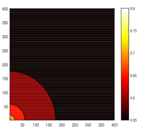
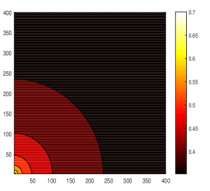
In the present simulation study, we restrict our attention to such a family of covariance functions. Specifically, we have considered the parameter values $\beta=\gamma=0.2,$ in the generations of Gaussian random field $X$ with covariance function (21) (see Figure 1). From ten independent copies $X_{i},$ $i=1,\dots,10,$ of random field $X$ a $\chi_{10}^{2}$ random field is also generated from the identity

$$\chi_{10}^{2}(\mathbf{x})=\frac{1}{2}\left[X_{1}^{2}(\mathbf{x})+\dots+X_{10}^{2}(\mathbf{x})\right],\mathbf{x}\in\mathbb{R}^{d}.$$

Its correlation function $\gamma$ is given by

$$\gamma(\|\mathbf{x}-\mathbf{y}\|)=\frac{\mbox{Cov}(\chi_{10}^{2}(\mathbf{x}),\chi_{10}^{2}(\mathbf{y}))}{\mbox{Var}(\chi_{10}^{2}(\mathbf{0}))}=B^{2}(\|\mathbf{z}\|),$$

where $B^{2}(\|\mathbf{z}\|)$ has been introduced in (21).

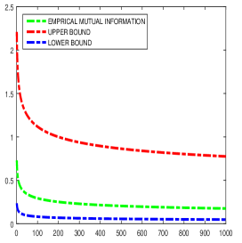
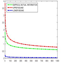
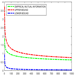
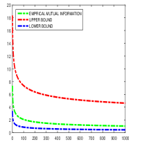
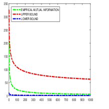
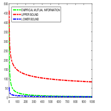
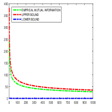
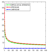
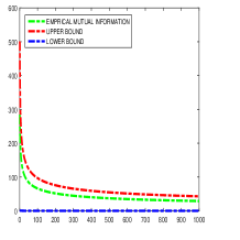
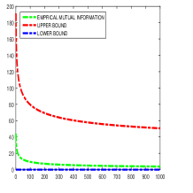
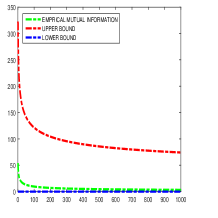
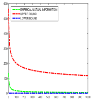
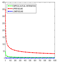
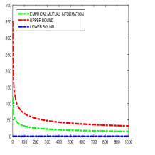
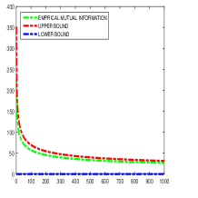
The results derived in Lemma 1, and Theorems 1 and 2 are illustrated for both models, computing Shannon and Rényi mutual informations for the corresponding original random variables, and for their transformed versions in terms of indicator functions, considering an increasing sequence of distances between the involved random variables. Specifically, a truncated version of $I(X(\mathbf{x}),X(\mathbf{y})),$ and $I_{q}(X(\mathbf{x}),X(\mathbf{y})),$ based on $M=5$ Hermite and Laguerre polynomials, respectively, is computed for spatial distances $d_{n}=\|\mathbf{x}_{n}-\mathbf{y}_{n}\|,$ $d_{n}=1,\dots,1000.$ The derived lower and upper bounds are represented as well. In particular, Figure 2 displays in green dashed line $I(X(\mathbf{x}),X(\mathbf{y}))$ (top-left), and $I(\chi_{10}^{2}(\mathbf{x}),\chi_{10}^{2}(\mathbf{y}))$ (top-right)$I(g(X(\mathbf{x})),g(X(\mathbf{y})))$ (bottom-left), and $I(g(\chi_{10}^{2}(\mathbf{x})),g(\chi_{10}^{2}(\mathbf{y})))$ (bottom-right). Here, $g(x)=1_{\nu}(x),$ $\nu=0.95.$ The upper and lower bounds are represented in dashed red and blue lines, respectively. The values of $I_{q}(X(\mathbf{x}),X(\mathbf{y})),$ $q=1.5,~{}2.10,~{}2.25;$ $I_{q}(\chi_{10}^{2}(\mathbf{x}),\chi_{10}^{2}(\mathbf{y})),$ $q=2,~{}2.05,~{}2.10;$ $I_{q}(g(X(\mathbf{x})),g(X(\mathbf{y}))),$ $q=1.5,~{}1.75,~{}1.95;$ and $I_{q}(g(\chi_{10}^{2}(\mathbf{x})),g(\chi_{10}^{2}(\mathbf{y}))),$ $q=1.75,~{}1.85,~{}1.95;$ for $g(x)=1_{\nu}(x),$ $\nu=0.95,$ are also plotted in Figure 3. It must be observed that, as we have checked through a large number of simulations, sensitivity at shorter distances with respect to the deformation parameter $q$ depends on the polynomial basis and the truncation order selected.

Refer to caption
Refer to caption
Figure 1: Covariance function of $X$ (left-hand side), and covariance function of $\chi_{10}^{2}$ (right-hand side) for a regular grid of $20\times 20$ spatial locations, with respect to distances in horizontal axis.
Refer to caption
Refer to caption
Refer to caption
Refer to caption
Figure 2: In green color, truncated $I(X(\mathbf{x}),X(\mathbf{y}))$ (top-left), and $I(\chi_{10}^{2}(\mathbf{x}),\chi_{10}^{2}(\mathbf{y}))$ (top-right), $I(g(X(\mathbf{x})),g(X(\mathbf{y})))$ (bottom-left), and $I(g(\chi_{10}^{2}(\mathbf{x})),g(\chi_{10}^{2}(\mathbf{y})))$ (bottom-right). The upper and lower bounds are represented in red and blue colors, respectively. Here, $g(x)=1_{\nu}(x),$ $\nu=0.95$
Refer to caption
Refer to caption
Refer to caption
Refer to caption
Refer to caption
Refer to caption
Refer to caption
Refer to caption
Refer to caption
Refer to caption
Refer to caption
Refer to caption
Figure 3: In green color, truncated $I_{q}(X(\mathbf{x}),X(\mathbf{y})),$ $q=1.5,~{}2.10,~{}2.25$ (top-row); $I_{q}(\chi_{10}^{2}(\mathbf{x}),\chi_{10}^{2}(\mathbf{y})),$ $q=2,~{}2.05,~{}2.10$ (second row); $I_{q}(g(X(\mathbf{x})),g(X(\mathbf{y}))),$ $q=1.5,~{}1.75,~{}1.95$ (third row), and $I_{q}(g(\chi_{10}^{2}(\mathbf{x})),g(\chi_{10}^{2}(\mathbf{y}))),$ $q=1.75,~{}1.85,~{}1.95,$ for $g(x)=1_{\nu}(x)$ (fourth row). The upper and lower bounds are represented in red and blue colors, respectively. As before, $g(x)=1_{\nu}(x),$ $\nu=0.95$

4 Spatiotemporal case: functional approach

In this section, we consider the extension of the above introduced concepts and elements in an infinite-dimensional framework. In this sense, a wider concept of diversity is adopted for functional systems characterized by separable non-countable families of infinite-dimensional random variables, and their measurable functions.

Specifically, the departure from independence of the components of a functional system, as displayed by spatial white noise random fields, is measured in terms of diversity loss in the spatial functional sample paths. Equivalently, diversity loss is induced here by the strong interrelations displayed by the functional random components of such systems.

4.1 Mutual information in an infinite-dimensional framework

The formulation of mutual information as a measure for spatiotemporal structural complexity analysis can be addressed for the general class of Lancaster-Sarmanov random fields adopting the infinite-dimensional spatial framework introduced in Angulo and Ruiz-Medina (2023).

Let $X=\{X_{\mathbf{x}}(\cdot),\ \mathbf{x}\in\mathbb{R}^{d}\}$ be a zero-mean homogeneous and isotropic spatial functional random field on the separable Hilbert space $(H,<\cdot,\cdot>_{H})$, mean-square-continuous w.r.t. the $H$ norm. In the following, we will assume that $H=L^{2}(\mathcal{T}),$ with $\mathcal{T}\subseteq\mathbb{R}_{+}$. For every $\mathbf{x},\mathbf{y}\in\mathbb{R}^{d}$, $\left(X_{\mathbf{x}}(\cdot),X_{\mathbf{y}}(\cdot)\right)^{T}$ is a random element in the separable Hilbert space $\left(H^{2},\left\langle\cdot,\cdot\right\rangle_{H^{2}}\right)$ of vector functions $\mathbf{f}=(f_{1},f_{2})^{T}$, with the inner product given by $\left\langle\mathbf{f},\mathbf{g}\right\rangle_{H^{2}}=\sum_{i=1}^{2}\left\langle f_{i},g_{i}\right\rangle_{H},\ \forall\mathbf{f},\mathbf{g}\in H^{2}$. Thus, for every $\mathbf{x},\mathbf{y}\in\mathbb{R}^{d}$, we consider the measurable function

$$\left(X_{\mathbf{x}}(\cdot),X_{\mathbf{y}}(\cdot)\right)^{T}:\;(\Omega,\mathcal{A},P)\longrightarrow\left(H^{2},\mathcal{B}(H^{2}),P_{\|\mathbf{x}-\mathbf{y}\|}(dh_{1},dh_{2})\right).$$

Let us denote by $\{P_{X_{\mathbf{x}}(\cdot)}(dh),\ \mathbf{x}\in\mathbb{R}^{d}\}$ the marginal infinite-dimensional probability distributions, with $P_{X_{\mathbf{x}}(\cdot)}(dh)=P(dh),$ for every $\mathbf{x}\in\mathbb{R}^{d}.$ Let $L^{2}(H,P(dh))$ be the space of measurable functions $g:\ H\longrightarrow\mathbb{R}$ such that $\int_{H}|g(h)|^{2}P(dh)<\infty.$ Assume that there exists an orthonormal basis $\{\mathcal{B}_{k},\ k\geq 0\}$ of $L^{2}(H,P(dh))$ such that the Radon-Nikodym derivative of the bivariate infinite-dimensional probability distribution $P_{\|\mathbf{x}-\mathbf{y}\|}(dh_{1},dh_{2})$ can be written in terms of the corresponding marginals as (see, e.g., Ledoux and Talagrand, 1991), for $n,m\geq 1,$

$\displaystyle p_{\|\mathbf{x}-\mathbf{y}\|,n,m}(h_{1},h_{2})=p(h_{1})p(h_{2})$
$\displaystyle\times\left[1+\sum_{k\geq 1}\left[\int_{H}\left\langle X_{\mathbf{x}}(\cdot),\phi_{n}(\cdot)\right\rangle_{L^{2}(\mathcal{T})}\left\langle X_{\mathbf{y}}(\cdot),\phi_{m}(\cdot)\right\rangle_{L^{2}(\mathcal{T})}P_{\|\mathbf{x}-\mathbf{y}\|}(dX_{\mathbf{x}}(\cdot),dX_{\mathbf{y}}(\cdot))\right]^{k}\right.$
$\displaystyle\hskip 142.26378pt\left.\times\mathcal{B}_{k}(h_{1})\mathcal{B}_{k}(h_{2})\right]\mu(dh_{1},dh_{2}),$

for a given orthonormal basis $\{\phi_{n},\ n\geq 1\}$ of $H,$ with

$\displaystyle\gamma_{\|\mathbf{x}-\mathbf{y}\|}(\phi_{n})(\phi_{m})=\mbox{Corr}(X_{\mathbf{x}}(\phi_{n}),X_{\mathbf{y}}(\phi_{m}))$
$\displaystyle=\int_{H}\left\langle X_{\mathbf{x}}(\cdot),\phi_{n}(\cdot)\right\rangle_{L^{2}(\mathcal{T})}\left\langle X_{\mathbf{y}}(\cdot),\phi_{m}(\cdot)\right\rangle_{L^{2}(\mathcal{T})}P_{\|\mathbf{x}-\mathbf{y}\|}(dX_{\mathbf{x}}(\cdot),dX_{\mathbf{y}}(\cdot))$

being the spatial correlation operator applied to the elements $\phi_{n}$ and $\phi_{m}$ of the orthonormal basis $\{\phi_{n},\ n\geq 1\},$ for every $\mathbf{x},\mathbf{y}\in\mathbb{R}^{d}.$ Here, $p(h)$ denotes the Radon-Nikodym derivative of the absolutely continuous marginal infinite–dimensional probability measure $P(dh),$ with respect to the uniform probability measure $\mu(dh)$ in $H.$ The bivariate uniform measure on $H^{2}$ is denoted as $\mu(dh_{1},dh_{2}).$

Under the above setting of conditions, the resulting class of spatial functional random fields defines the infinite–dimensional version of Lancaster-Sarmanov random fields. In the simulation study undertaken in the next section, we analyze the asymptotic behavior of the Shannon entropy based mutual information between two random components of an element of this functional random field class. Specifically, from the infinite-dimensional formulation of Kullback-Leibler divergence established in Angulo and Ruiz-Medina (2023), we consider the following version of Shannon mutual information operator as a functional counterpart of equation (9): For $\mathbf{x},\mathbf{y}\in\mathbb{R}^{d}$, and $n,m\geq 1,$

$\displaystyle\mathcal{S}_{\varrho}(\|\mathbf{x}-\mathbf{y}\|,n,m):=\mathcal{S}_{\varrho}(\|\mathbf{x}-\mathbf{y}\|)(\phi_{n})(\phi_{m})$
$\displaystyle\int_{H^{2}}P_{\|\mathbf{x}-\mathbf{y}\|,n,m}(dh_{1},dh_{2})\ln\left(\frac{p_{\|\mathbf{x}-\mathbf{y}\|,n,m}(h_{1},h_{2})}{p(h_{1})p(h_{2})}\right)$
$\displaystyle=\int_{H^{2}}p(h_{1})~{}p(h_{2})~{}\left[1+\sum_{k=1}^{\infty}[\gamma_{\|\mathbf{x}-\mathbf{y}\|}(\phi_{n})(\phi_{m})]^{k}\right.$
$\displaystyle\left.\times\mathcal{B}_{k}(h_{1})\mathcal{B}_{k}(h_{2})\right]\ln\left(1+\sum_{k=1}^{\infty}[\gamma_{\|\mathbf{x}-\mathbf{y}\|}(\phi_{n})(\phi_{m})]^{k}~{}\mathcal{B}_{k}(h_{1})\mathcal{B}_{k}(h_{2})\right)\mu(dh_{1},dh_{2}).$

4.2 Simulation study

Let $\varphi(u)$, $u\geq 0$, be a completely monotone function, and suppose further that $\psi(u)$, $u\geq 0$, is a positive function with a completely monotone derivative (such functions are also called Bernstein functions). Consider the function

$$C(\left\|z\right\|,\tau)=\frac{\sigma^{2}}{[\psi(\tau^{2})]^{d/2}}\varphi\left(\frac{\left\|z\right\|^{2}}{\psi(\tau^{2})}\right),\text{ }\sigma^{2}\geq 0,\text{ }(z,\tau)\in\mathbb{R}^{d}\times\mathbb{R}.$$ (24)

Hence $C$ is a covariance function under Gneiting’s criterion (see Gneiting, 2002). Let now consider the special case of functions $\varphi$ and $\psi$ given by

$\displaystyle\varphi(u)$ $\displaystyle=$ $\displaystyle\frac{1}{(1+cu^{\gamma})^{\delta}},u>0,c>0,0<\gamma\leq 1,\delta>0$
$\displaystyle\psi(u)$ $\displaystyle=$ $\displaystyle(1+au^{\alpha})^{\beta},\text{ }a>0,\text{ }0<\alpha\leq 1,\text{ }0<\beta\leq 1,\text{ }u\geq 0.$ (25)

Note that, functions $\varphi$ and $\psi$ can also be written as

$\displaystyle\varphi(u)$ $\displaystyle=$ $\displaystyle\frac{\mathcal{L}_{1}(u)}{u^{\gamma\delta}},\quad\mathcal{L}_{1}(u)=\frac{u^{\gamma\delta}}{(1+cu^{\gamma})^{\delta}}$
$\displaystyle\psi(u)$ $\displaystyle=$ $\displaystyle\left[\frac{\mathcal{L}_{2}(u)}{u^{\alpha\beta}}\right]^{-1},\quad\mathcal{L}_{2}=\frac{u^{\alpha\beta}}{(1+au^{\alpha})^{\beta}},$ (26)

where $\mathcal{L}_{i},$ $i=1,2,$ represent positive continuous slowly varying function at infinity, satisfying

$$\lim_{T\to\infty}\frac{\mathcal{L}_{i}\left(T\|z\|\right)}{\mathcal{L}\left(T\right)}=1,\quad i=1,2,$$ (27)

for every $z\in\mathbb{R}^{d},$ $d\geq 1.$

Applying Tauberian Theorems (see Doukhan et al., 1996; see also Theorems 4 and 11 in Leonenko and Olenko, 2014), their Fourier transforms satisfy

$\displaystyle\widehat{\varphi}(\lambda)=\int_{\mathbb{R}^{d}}\exp\left(-i\left\langle\lambda,z\right\rangle\right)\varphi(\|z\|^{2})dz$ $\displaystyle\sim$ $\displaystyle c(1,2\gamma\delta)\frac{\mathcal{L}_{1}\left(\frac{1}{\|\lambda\|}\right)}{\|\lambda\|^{d-2\gamma\delta}},\quad\mbox{as }\|\lambda\|\to 0$
$\displaystyle\widehat{\psi}(\omega)=\int_{\mathbb{R}}\exp\left(-i\left\langle\omega,t\right\rangle\right)\psi(|t|^{2})dt$ $\displaystyle\sim$ $\displaystyle c(1,2\alpha\beta)\frac{\mathcal{L}_{2}\left(\frac{1}{|\omega|}\right)}{|\omega|^{1-2\alpha\beta}},\quad\mbox{as }|\omega|\to 0,$

where $c\left(d,\theta\right)=\frac{\Gamma\left(\frac{d-\theta}{2}\right)}{\pi^{d/2}2^{\theta}\Gamma(\theta/2)},$ with $\theta=2\gamma\delta,$ and $\theta=2\alpha\beta,$ for $0<2\gamma\delta<d,$ and $0<2\alpha\beta<1.$

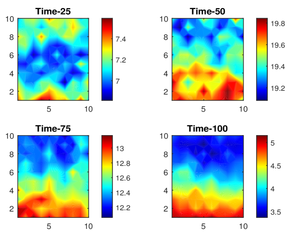
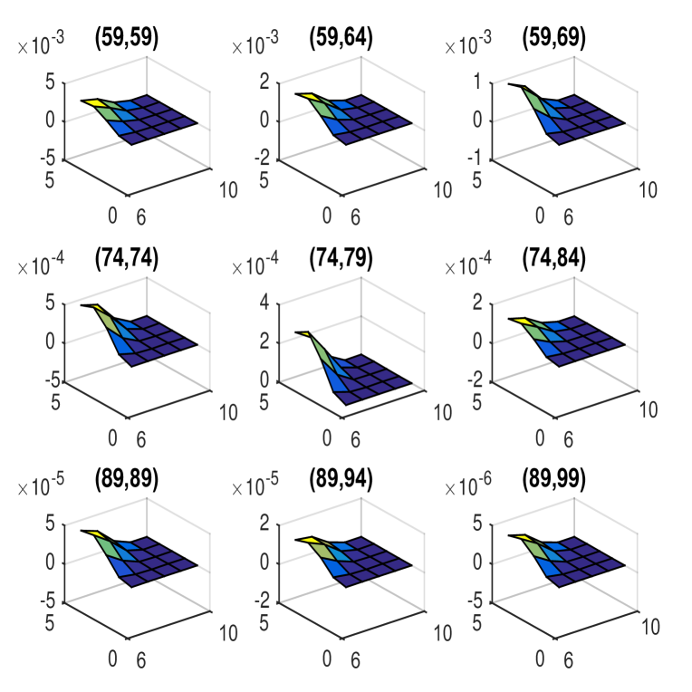
Figure 4 displays color plots surfaces of the Gaussian spatiotemporal random field, generated with covariance function in the Gneiting class for $\alpha=0.3,$ $\beta=0.7,$ $\gamma=0.2,$ and $\delta=0.35,$ at times $t=25,50,75,100.$ Shannon mutual information surfaces are evaluated from the reconstruction formula

$$\mathcal{K}_{\mathcal{S}_{\|\mathbf{x}-\mathbf{y}\|}}(t,s)=\sum_{n=1}^{M}\sum_{m=1}^{M}\mathcal{S}_{\varrho}(\|\mathbf{x}-\mathbf{y}\|)(\phi_{n})(\phi_{m})\phi_{n}\otimes\phi_{m}(t,s)$$

implemented for $M=100.$ Figure 4 displays spatial cross–sections $\mathcal{K}_{\mathcal{S}_{\|\mathbf{x}_{i}-\mathbf{y}_{i}\|}}(t,s)$ corresponding to spatial nodes $(i,1),$ $i=1,2,3,4,5$ (labeled at the x-axis), and $(i,1),$ $i=6,7,8,9,10$ (labeled at the y-axis), at $(t,s)\in[1,100]\times[1,100].$ It can be observed the same power law in the decay of $\mathcal{K}_{\mathcal{S}_{\|\mathbf{x}-\mathbf{y}\|}}(t,s)$ as $\|\mathbf{x}-\mathbf{y}\|\to\infty,$ for each fixed $(t,s)\in[1,100]\times[1,100].$

Refer to caption
Figure 4: The surfaces values at times $t=25,50,75,100$ of the Gaussian spatiotemporal random field generated with covariance function in the Gneiting class are displayed
Refer to caption
Figure 5: Shannon mutual information surfaces corresponding to crossing two random components respectively located at spatial nodes $(i,1),$ $i=1,2,3,4,5$ (values labeled at the x-axis), and $(i,1),$ $i=6,7,8,9,10$ (values labeled at the y-axis) of the $10\times 10$ spatial regular grid considered, for crossing times in the set $\left[\{59,\dots,99\}\right]^{2}.$

5 Conclusion

This paper focuses on the asymptotic mutual information based analysis of a class of spatial and spatiotemporal LRD Lancaster-Sarmanov random fields and their subordinated. Persistence of memory in space is characterized in terms of the LRD parameter, modelling the mutual information decay representing spatial structure dissipation at large scales. Random field subordination affects this decay rate when the rank $m$ of the function $g$ involved in the subordination is larger than one. Hence, large scale aggregation is lost up to order $m.$ Faster decay to zero is then observed in the corresponding asymptotic order modeling a faster spatial structure dissipation from intermediate scales. However, when the rank is equal to one, as illustrated here in the case of $g$ being the indicator function, spatial structure dissipation occurs at the same rate, for the original and transformed random variables. The structural index provided by Rényi mutual information reflects some different behaviors depending on the characteristics of the polynomial basis (in our simulation study, Hermite or Laguerre polynomials), as well as on the range analyzed for the $q$ deformation parameter. Particularly, this range induces strong changes at small spatial scales, but the general shape of the curves reflecting asymptotic decay is invariant, and displays a power law involving the LRD and the deformation parameters.

In the spatiotemporal case, the class of Lancaster-Sarmanov random fields is introduced in a spatial functional framework. The simulation study undertaken shows a similar asymptotic behavior at spatial macroscale level, i.e., power law decay of the mutual information surfaces, which is accelerated at coarser temporal scales. Thus, time varying asymptotic orders are obtained characterizing the spatial diversity loss in a functional framework, under an increasing domain asymptotics. Similar results will be derived, in a subsequent paper, regarding the asymptotic analysis of Shannon and Rényi mutual information measures, in an infinite-dimensional framework, in terms of time-varying spatial local complexity orders associated with a fixed domain asymptotics, reflecting limiting behaviors at high resolution levels.

Acknowledgements

This work has been supported in part by grants PGC2018-098860-B-I00 (J.M. Angulo), PGC2018-099549-B-I00 (M.D. Ruiz-Medina) and PID2021-128077NB-I00 (J.M. Angulo) funded by MCIN / AEI/10.13039/501100011033 / ERDF A way of making Europe, EU, and grant CEX2020-001105-M funded by MCIN / AEI/10.13039/501100011033.

References

  • [1] Alonso, F.J., Bueso, M.C., Angulo, J.M., 2016. Dependence assessment based on generalized relative complexity: Application to sampling network design. Methodology and Computing in Applied Probability 18, 921-933.
  • [2] Angulo, J.M., Esquivel, F.J, Madrid, A.E., Alonso, F.J., 2021. Information and complexity analysis of spatial data. Spatial Statistics 42, 100462.
  • [3] Angulo, J.M., Ruiz-Medina, M.D., 2023. Infinite-dimensional divergence information analysis. In: Trends in Mathematical, Information and Data Sciences, N. Balakrishnan, M.A. Gil, N. Martín, D. Morales, M.C. Pardo (eds.), 147-157. Studies in Systems, Decision and Control 445. Springer (in press).
  • [4] Bosq, D., 2000 Linear Processes in Function Spaces. Springer-Verlag, New York.
  • [5] Bulinski, A., Spodarev, E., Timmermann, F., 2012. Central limit theorems for the excursion volumes of weakly dependent random fields. Bernoulli 18, 100-118.
  • [6] Campbell, L.L., 1966. Exponential entropy as a measure of extent of a distribution. Zeitschrift für Wahrscheinlichkeitstheorie und Verwandte Gebiete 5,217-225.
  • [7] Da Prato, G., Zabczyk, J., 2002. Second Order Partial Differential Equations in Hilbert Spaces. Cambridge University Press, Cambridge, New York.
  • [8] Doukhan, P., León, J.R, Soulier, P., 1996. Central and non-central limit theorems for quadratic forms of a strongly dependent Gaussian field. Brazilian Journal of Probability and Statistics 10, 205-223.
  • [9] Ferraty, F., Vieu, P., 2006. Nonparametric Functional Data Analysis: Theory and Practice. Springer, New York.
  • [10] Frías, M.P., Torres-Signes, A., Ruiz-Medina, M.D., 2022. Spatial Cox processes in an infinite-dimensional framework. Test 31, 175-203.
  • [11] Gneiting, T., 2002. Nonseparable, stationary covariance functions for space-time data. Journal of the American Statistical Association 97, 590-600.
  • [12] Ivanov, A.V., Leonenko, N.N., 1989. Statistical Analysis of Random Fields. Kluwer Academic, Dordrecht.
  • [13] Kullback, S., Leibler, R.A. 1951. On information and sufficiency. The Annals of Mahematical Statistics 22, 79-86.
  • [14] Lancaster, H.O., 1958. The structure of bivariate distributions. The Annals of Mathematical Statistics 29, 719-736.
  • [15] Ledoux, M., Talagrand, M., 1991. Probability in Banach Spaces. Springer, Heidelberg.
  • [16] Leonenko, N.N., 1999. Limit Theorems for Random Fields with Singular Spectrum. Mathematics and its Applications 465. Kluwer Academic, Dordrecht.
  • [17] Leonenko, N.N., Olenko, A., 2014. Sojourn measures of Student and Fisher-Snedecor random fields. Bernoulli 20, 1454-1483.
  • [18] Leonenko, N.N., Ruiz-Medina, M.D., 2022. Sojourn functionals for spatiotemporal Gaussian random fields with long-memory. Advances in Applied Probability (in press).
  • [19] Leonenko, N.N., Ruiz-Medina, M.D., Taqqu, M.S., 2017. Non-central limit theorems for random fields subordinated to Gamma-correlated random fields. Bernoulli 23, 3469-3507.
  • [20] López-Ruiz, R., Nagy, Á., Romera, E., Sañudo, J., 2009. A generalized statistical complexity measure: Applications to quantum systems. Journal of Mathematical Physics 50, 123528.
  • [21] Makogin, V., Spodarev, E., 2022. Limit theorems for excursion sets of subordinated Gaussian random fields with long-range dependence. Stochastics 94, 111-142.
  • [22] Marinucci, D., Peccati, G., 2011. Random Fields on the Sphere. Representation, Limit Theorems and Cosmological Applications. London Mathematical Society Lecture Note Series 389. Cambridge University Press, Cambridge.
  • [23] Peccati, G., Taqqu, M.S., 2011. Wiener Chaos: Moments, Cumulants and Diagrams. Springer, New York.
  • [24] Rényi, A., 1961. On measures of entropy and information. In: Proceedings of the Fourth Berkeley Symposium on Mathematical Statistics and Probability, Berkeley, CA, USA, June 20-July 30 1960, J. Neyman (ed.) Vol. 1, 547-561. University of California Press, Berkeley.
  • [25] Romera, E., Sen, K.D., Nagy, Á., 2011. A generalized relative complexity measure. Journal of Statistical Mechanics: Theory and Experiment 2011(9), P09016.
  • [26] Ruiz-Medina, M.D., 2022. Spectral analysis of long range dependence functional time series. Fractional Calculus and Applied Analysis 25, 1426-1458.
  • [27] Sarmanov, O.V., 1963. Investigation of stationary Markov processes by the method of eigenfunction expansion. Selected Translations in Mathematical Statistics and Probability 4, 245-269.
  • [28] Shannon, C.E., 1948. A mathematical theory of communication. The Bell System Technical Journal 27, 379-423.
  • [29] Simon, T., 2014. Comparing Fréchet and positive stable laws. Electronic Journal of Probability 19, 1-25.
  • [30] Torres-Signes, A., Frías, M.P., Ruiz-Medina, M.D., 2021. COVID-19 mortality analysis from soft-data multivariate curve regression and machine learning. Stochastic Environmental Research and Risk Assessment 35, 2659-2678.