Principled and Efficient Transfer Learning of Deep Models via Neural Collapse

Abstract

As model size continues to grow and access to labeled training data remains limited, transfer learning has become a popular approach in many scientific and engineering fields. This study explores the phenomenon of neural collapse (NC) in transfer learning for classification problems, which is characterized by the last-layer features and classifiers of deep networks having zero within-class variability in features and maximally and equally separated between-class feature means. Through the lens of NC, in this work the following findings on transfer learning are discovered: (i) preventing within-class variability collapse to a certain extent during model pre-training on source data leads to better transferability, as it preserves the intrinsic structures of the input data better; (ii) obtaining features with more NC on downstream data during fine-tuning results in better test accuracy. These results provide new insight into commonly used heuristics in model pre-training, such as loss design, data augmentation, and projection heads, and lead to more efficient and principled methods for fine-tuning large pre-trained models. Compared to full model fine-tuning, our proposed fine-tuning methods achieve comparable or even better performance while reducing fine-tuning parameters by at least 70% as well as alleviating overfitting.

1 Introduction

Transfer learning has gained widespread popularity in computer vision, medical imaging, and natural language processing [1, 2, 3]. By taking advantage of domain similarity, a pre-trained, large model from source datasets is reused as a starting point or feature extractor for fine-tuning a new model on a smaller downstream task [1]. The reuse of the pre-trained model during fine-tuning reduces computational costs significantly and leads to superior performance on problems with limited training data.

However, without principled guidance, the underlying mechanism of transfer learning is not well understood. First, when pre-training deep models on the source dataset, there are no good metrics to measure the quality of the learned model or representation in terms of transferability. In the past, people used to rely on controversial metrics, such as validation accuracy on the pre-trained data (e.g., validation accuracy on ImageNet [4]), to predict test performance on downstream tasks. However, some popular methods for boosting ImageNet validation accuracy, such as label smoothing [5] and dropout [6], have been shown to harm (rather than boost) transfer performance on downstream tasks [7]. On the other hand, the design of loss functions [7, 8], data augmentations [9], increased model size, and projection head layers [9] to improve transferability are often based on trial and error without much understanding of the underlying mechanism. Second, due to the size of models (e.g., GPT-3 and transformer [10, 11, 2, 12]), efficient fine-tuning on downstream tasks remains a big challenge but is crucial for large models [13, 14, 15]. Full fine-tuning of the pre-trained model parameters often results in the best performance, but it becomes increasingly expensive with larger models and often leads to overfitting due to limited downstream data. These challenges highlight the need for a deeper understanding of what makes pre-trained deep models more transferable.

Figure 1: An illustration of neural collapse. Here dots $\bullet$ represent training samples, crosses $\times$ stand for the testing samples, and $\phi_{\bm{\theta}}(\cdot):\mathbb{R}^{D}\rightarrow\mathbb{R}^{d}$ represents the feature mapping of the network, meaning the output of the second-to-last layer.

In this work, we examine the fundamental principles of transfer learning based on a recent discovery in last-layer representations referred to as “Neural Collapse” ($\mathcal{NC}$) [16, 17], where the last-layer features and classifiers “collapse” to simple while elegant mathematical structures on the training data. Specifically, (i) the within-class variability of last-layer features collapses to zero for each class and (ii) the between-class means and last-layer classifiers collapse to the vertices of a Simplex Equiangular Tight Frame (ETF) up to a scaling. This $\mathcal{NC}$ phenomenon has been observed across different network architectures and datasets [16, 17]. Moreover, under simplified unconstrained feature models [18, 19], recent works have explained the prevalence of $\mathcal{NC}$ for training overparameterized deep networks, across various training losses [20, 21, 22, 23] and problem formulations [19, 24, 25]. Despite these efforts, a critical question remains: is $\mathcal{NC}$ a blessing or a curse for deep representation learning? This work seeks to address this question within the context of transfer learning.

1.1 Contributions of This Work

In this work, we study the transferability of pre-trained models through the lens of $\mathcal{NC}$. Because $\mathcal{NC}$ results in the reduction of within-class feature variability, the learned representations fails to preserve the intrinsic dimensionality of the input data. This can lead to poor transferability in vanilla supervised learning. To ensure transferability during model pre-training, it is important for the learned features of each class to be not only discriminative but also diverse, to preserve the intrinsic structures of the input data. Conversely, during fine-tuning on the downstream task, we aim for greater collapse of the features on the downstream training data.

Based on these intuitions, we adapt the metrics for evaluating $\mathcal{NC}$ to measure the quality of learned representations in terms of both within-class diversity and between-class discrimination. This approach not only helps us understand several commonly used heuristics in transfer learning, but it also leads to more systematic and efficient methods for fine-tuning large pre-trained models on downstream data. In summary, our empirical findings using the $\mathcal{NC}$ metrics can be highlighted as follows.

• Less collapsed features on source data leads to better transferability to certain extents. We evaluated the $\mathcal{NC}$ metrics on different loss functions [26] and various techniques in transfer learning, such as the projection head [9], data augmentations [27, 8], and adversarial training [28, 29]. We found that the more diverse the features are, the better the transferability of the pre-trained model. As such, our findings explain the underlying mechanism of many popular heuristics in model pre-training. Additionally, we found that the relationship between feature diversity and transfer accuracy only holds to a certain extent, as randomly generated features that are not collapsed do not generalize well.

• More collapsed features on downstream tasks result in better transfer accuracy. Our evaluation of different pre-trained models on downstream tasks shows that greater collapse of features on the downstream data generally leads to better transfer accuracy; a similar phenomenon also happens for few-shot learning. For transfer learning, such a phenomenon has been demonstrated to be universal across various downstream datasets [30, 31, 32, 33] and pre-trained models [34, 12, 35, 36]. Furthermore, we showed that this phenomenon also occurs across different layers of the same pre-trained model.

• More efficient fine-tuning of large pre-trained models via $\mathcal{NC}$. Based on our above findings, we propose a simple but memory-efficient fine-tuning method: we only fine-tune one key layer with skip connection to collapse the features of the penultimate layer. Our experiments with various network architectures show that the proposed fine-tuning strategy performs equally well or even better than full model fine-tuning. In the scenario of limited downstream data, our method demonstrates greater resilience to data scarcity and less overfitting.

1.2 Relationship to Prior Art

The occurrence of the Neural Collapse ($\mathcal{NC}$) phenomenon has recently received significant attention in both practical and theoretical fields, and our work explores the link between $\mathcal{NC}$ and transfer learning. Prior to our work, several recent studies have also examined the properties of deep representations for transfer learning, which are also relevant to our work. Below, we provide a summary and brief discussion of these results.

• Understanding the Neural Collapse Phenomenon. Recently, several studies have focused on deciphering the training, generalization, and transferability of deep networks in terms of $\mathcal{NC}$; see a recent review paper [37]). With regards to training, recent studies have shown that $\mathcal{NC}$ occurs with a variety of loss functions and formulations, including cross-entropy (CE) [16, 38, 20, 19, 39, 25], mean-squared error (MSE) [18, 17, 22, 24, 40, 41], and supervised contrastive (SupCon) losses [21]. In terms of generalization, the study in [42] has shown that $\mathcal{NC}$ also occurs on test data drawn from the same distribution asymptotically, but less severe with limited finite test samples [43]. Several recent works [16, 42, 43] have studied the connection between $\mathcal{NC}$ and generalization of overparameterized deep networks. In addition, [43, 44, 45] have demonstrated that feature variability collapses progressively from shallow to deep layers (with a linear decay rate [45]), and [46] showed that test performance can be improved by enforcing variability collapse on intermediate layer features. The line of work [19, 47, 48, 49, 50, 51, 52] investigated the connections between imbalanced training and $\mathcal{NC}$, where [48] showed that fixing the classifier as simplex ETFs enhances test performance on imbalanced training and long-tailed classification problems. Finally, the study in [7] has implicitly shown that there is a tradeoff between feature variability collapse and transfer accuracy through experiments with various loss functions.

• Representation Learning and Model Pre-training. The factors affecting the transferability of pre-trained models have been studied in a number of recent works, but the conclusions are not entirely clear. The work in [4] suggests that models pre-trained on ImageNet with higher accuracy tend to perform better on other downstream tasks. However, this conclusion has been challenged by more recent works such as [7, 53], which showed that the training loss and feature diversity may be more important factors in transferability than pre-training accuracy. Moreover, compared to our work, these works only study a limited number of aspects that affect transferability, focusing only on the diversity of the source dataset. On the other hand, [54] found that models learned using contrastive loss functions have better transferability and [55] found that their representations are more uniform over hyperspheres. The architecture and depth of convolutional neural networks (CNN) have also been shown to impact transfer performance [56]. Additionally, the result in [57] highlights the importance of layers in overparameterized networks, which suggests that shallow and deep layers are crucial in fine-tuning pre-trained models for downstream tasks.

1.3 Notations & Organization

Throughout the paper, we use bold lowercase and upper letters, such as $\bm{A}$ and $\bm{A}$, to denote vectors and matrices, respectively. Not-bold letters are reserved for scalars. The symbols $\bm{I}_{K}$ and $\bm{1}_{K}$ respectively represent the identity matrix and the all-ones vector with an appropriate size of $K$, where $K$ is some positive integer. We use $[K]:=\left\{1,2,\dots,K\right\}$ to denote the set of all indices up to $K$. For any matrix $\bm{A}\in\mathbb{R}^{n_{1}\times n_{2}}$, we write $\bm{A}=\begin{bmatrix}\bm{a}_{1}&\dots&\bm{a}_{n_{2}}\end{bmatrix}$, so that $\bm{a}_{i}$ ($i\in[n_{2}]$) denote a column vector of $\bm{A}$.

The rest of the paper is organized as follows. In Section 2, we provide a review of neural collapse and introduce metrics for measuring the discrimination and diversity of learned representations to evaluate transferability. In Section 3, we conduct extensive experiments using the metrics to demystify the heuristics used in model pre-training and provide guiding principles for model fine-tuning. Finally, we conclude the work in Section 4. Additional experimental details are included in the appendices.

2 Evaluating Representations of Pretrained Models via $\mathcal{NC}$

In this section, we first provide a brief overview of the $\mathcal{NC}$ phenomenon, followed by the introduction of metrics for evaluating the quality of learned representations for transfer learning. We end this section by a discussion of progressive collapse phenomenon across layers, which is crucial for our investigation in Section 3.

2.1 Basics of Deep Neural Networks

Let us first introduce some basic notations by considering a multi-class (e.g., $K$ class) classification problem with finite training samples. Let $\left\{n_{k}\right\}_{k=1}^{K}$ be the number of training samples in each class. Let $\bm{x}_{k,i}$ denote the $i$th input data in the $k$th class ($i\in[n_{k}]$, $k\in[K]$), and the corresponding one-hot training label is represented by $\mathbf{y}_{k}\in\mathbb{R}^{K}$, with only the $k$th entry equal to $1$. Thus, given any input data $\bm{x}_{k,i}$, we learn a deep network to fit the corresponding (one-hot) training label $\bm{y}_{k}$ such that

$$\bm{y}_{k}\;\approx\;\psi_{\bm{\Theta}}(\bm{x}_{k,i})\;=\;\underset{\text{\bf linear classifier}\;\bm{W}}{\bm{W}_{L}}\;\cdot\;\underset{\text{ \bf feature}\;\;\bm{h}_{k,i}\;=\;\phi_{\bm{\theta}}(\bm{x}_{k,i})}{\sigma\left(\bm{W}_{L-1}\cdots\sigma\left(\bm{W}_{1}\bm{x}_{k,i}+\bm{b}_{1}\right)+\bm{b}_{L-1}\right)}+\bm{b}_{L},$$ (1)

where $\bm{W}=\bm{W}_{L}$ represents the last-layer linear classifier and $\bm{h}_{k,i}=\bm{h}(\bm{x}_{k,i})=\phi_{\bm{\theta}}(\bm{x}_{k,i})$ is a deep hierarchical representation (or feature) of the input $\bm{x}_{k,i}$. Here, for a $L$-layer deep network $\psi_{\bm{\Theta}}(\bm{x})$, each layer is composed of an affine transformation, followed by a nonlinear activation $\sigma(\cdot)$ and normalization functions (e.g., BatchNorm [58]). We use $\bm{\Theta}$ to denote all the network parameters of $\psi_{\bm{\Theta}}(\bm{x})$ and $\bm{\theta}$ to denote the network parameters of $\phi_{\bm{\theta}}(\bm{x})$. Additionally, we use

$$\bm{H}\;=\;\begin{bmatrix}\bm{H}_{1}&\bm{H}_{2}&\cdots&\bm{H}_{K}\end{bmatrix}\in\mathbb{R}^{d\times N},\quad\bm{H}_{k}\;=\;\begin{bmatrix}\bm{h}_{k,1}&\cdots&\bm{h}_{k,n}\end{bmatrix}\in\mathbb{R}^{d\times n},\;\forall\;k\in[K],$$

to represent all the features in matrix form. Additionally, the class mean for each class is written as

$$\overline{\bm{H}}\;:=\;\begin{bmatrix}\overline{\bm{h}}_{1}&\cdots&\overline{\bm{h}}_{K}\end{bmatrix}\in\mathbb{R}^{d\times K}\quad\text{and}\quad\overline{\bm{h}}_{k}\;:=\;\frac{1}{n_{k}}\sum_{i=1}^{n_{k}}\bm{h}_{k,i},\quad;\forall\;k\in[K].$$

Accordingly, we denote the global mean of $\bm{H}$ as $\bm{h}_{G}=\frac{1}{K}\sum_{k=1}^{N}\overline{\bm{h}}_{k}$.

2.2 A Review of Neural Collapse in Terminal Phase of Training

It has been widely observed that the last-layer features $\mathbf{H}$ and classifiers $\mathbf{W}$ of a trained network on a balanced training dataset $\left\{\bm{x}_{k,i},\bm{y}_{k}\right\}$ with $n=n_{1}=n_{2}=\cdots=n_{K}$ exhibit simple but elegant mathematical structures [16, 44]. Here, we highlight two key properties below.

• Within-class variability collapse. For each class, the last-layer features collapse to their means,

  $$\bm{h}_{k,i}\rightarrow\overline{\bm{h}}_{k},\quad\forall\;1\leq i\leq n,\;1\leq k\leq K.$$ (2)

• Maximum between-class separation. The class-means ${\overline{\mathbf{h}}k}{k=1}^{K}$ centered at their global mean $\mathbf{h}_{G}$ are not only linearly separable but also maximally distant and form a Simplex Equiangular Tight Frame (ETF): for some $c>0$, $\overline{\bm{H}}=\begin{bmatrix}\overline{\bm{h}}_{1}-\bm{h}_{G}&\cdots&\overline{\bm{h}}_{K}-\bm{h}_{G}\end{bmatrix}$ satisfies

  $$\overline{\bm{H}}^{\top}\overline{\bm{H}}\;=\;\frac{cK}{K-1}\left(\bm{I}_{K}-\frac{1}{K}\bm{1}_{K}\bm{1}_{K}^{\top}\right).$$ (3)

Recent studies have shown that $\mathcal{NC}$ is prevalent across a wide range of classification problems, regardless of the loss function used (e.g., CE [16, 19], MSE [18, 22, 17], or SupCon [19, 21]), the neural network architecture (e.g., VGG [59], ResNet [34], or DenseNet [35]), and the dataset (e.g., MNIST [60], CIFAR [30], or ImageNet [61]). Although maximum between-class separation implies that the learned features are discriminative, the collapse of within-class variability to a single dimension (as shown in Equation 2) implies that the network is memorizing the labels instead of preserving the intrinsic structures of the data. This loss of information from the input to the output could negatively impact the transferability of the learned deep models. Nonetheless, the $\mathcal{NC}$ phenomenon provides useful metrics for evaluating the transferability of pre-trained models, which we will discuss further in the following.

2.3 Measuring Representation Quality via $\mathcal{NC}$ Metrics

Based on the above discussion, we can assess the transferability of pre-trained models by measuring the feature diversity and separation using metrics for evaluating $\mathcal{NC}$ [16, 20] defined as follows:

$$\mathcal{NC}_{1}\;:=\;\frac{1}{K}\operatorname{trace}\left(\bm{\Sigma}_{W}\bm{\Sigma}_{B}^{\dagger}\right).$$ (4)

More specifically, it measures the magnitude of the within-class covariance matrix $\bm{\Sigma}_{W}\in\mathbb{R}^{d\times d}$ of the learned features compared to the between-class covariance matrix $\bm{\Sigma}_{B}\in\mathbb{R}^{d\times d}$, where

$$\bm{\Sigma}_{W}\;:=\;\frac{1}{nK}\sum_{k=1}^{K}\sum_{i=1}^{n}\left(\bm{h}_{k,i}-\overline{\bm{h}}_{k}\right)\left(\bm{h}_{k,i}-\overline{\bm{h}}_{k}\right)^{\top},\quad\bm{\Sigma}_{B}\;:=\;\frac{1}{K}\sum_{k=1}^{K}\left(\overline{\bm{h}}_{k}-\bm{h}_{G}\right)\left(\overline{\bm{h}}_{k}-\bm{h}_{G}\right)^{\top}.$$

Here, $\bm{\Sigma}_{B}^{\dagger}$ represents the pseudo-inverse of $\bm{\Sigma}_{B}$, which normalizes $\bm{\Sigma}_{W}$ to capture the relative relationship between the two covariances. Essentially, if the features of each class are more closely clustered around their corresponding class means, $\mathcal{NC}_{1}$ will be smaller. Conversely, if the class means are more separated, $\mathcal{NC}_{1}$ will also be smaller for the same $\bm{\Sigma}_{W}$. However, computing this metric in (4) can be computationally expensive due to the pseudo-inverse, which is often the case for large models. To address this issue, alternative metrics such as class-distance normalized variance (CDNV) [42] and numerical rank [22] have been introduced recently; we refer interested readers to Appendix A for more details.

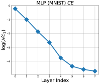
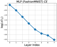
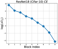
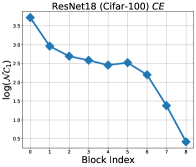
(a) CE

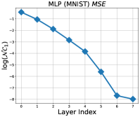
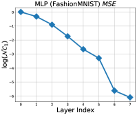
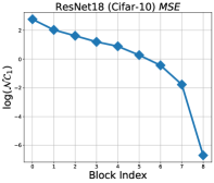
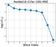
(b) MSE

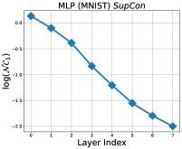
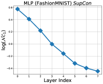
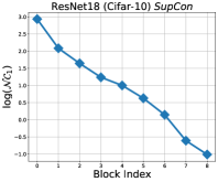
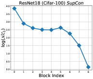
(c) SupCon

Figure 2: Decrease of the $\mathcal{NC}_{1}$ metric for trained MLP/ResNet18 Models with different losses. The MLP models were trained on the MNIST [60] and FashionMNIST [62] datasets, respectively. The ResNet18 models were trained on the Cifar-10 and Cifar-100 datasets. Similar results with progressive decay of $\mathcal{NC}_{1}$ across layers on MLP have been reported in previous studies using the CE loss on different datasets [16, 43, 45]; specifically, [45] showed linear convergence of $\mathcal{NC}_{1}$ across layers.

2.4 Progressive Collapse Across Layers

So far, various works [16, 17] have shown that the $\mathcal{NC}_{1}$ metric converges to zero when evaluated on the last-layer features $\bm{h}$. More surprisingly, when $\mathcal{NC}_{1}$ is evaluated on the features of intermediate layers, such as

$$\bm{h}^{\ell}\;:=\;\sigma\left(\bm{W}_{\ell-1}\cdots\sigma\left(\bm{W}_{1}\bm{x}+\bm{b}_{1}\right)+\bm{b}_{\ell-1}\right),\quad\forall\ell\in[L-1],$$

the $\mathcal{NC}$₁ quantity on the $\ell$-th layer ($\ell\in[L-1]$) is improved by roughly an equal multiplicative factor compared to the previous $\ell-1$-th layer [44, 43, 45]; see Figure 2 for an illustration.

Similar to the last-layer $\mathcal{NC}$, layer-wise progressive collapse is also a common occurrence across different training losses, network architectures, and datasets [45]. Furthermore, recent research [45] shows that the decay rate can be linear for simple networks such as MLPs, VGGs, and ResNets. The gradual decrease in feature diversity implies that the deep network is enhancing data separation and discarding input information as it progresses from shallow to deep layers. By utilizing this progressive collapse phenomenon, in the following we will show that we can gain a deeper understanding of various commonly used heuristic methods in pre-training deep models as well as develop more efficient fine-tuning methods based on principles.

3 Methods & Experiments

In this section, we will evaluate the quality of learned representations for transfer learning using the metric in (4). We will provide new insights into model pre-training and fine-tuning. Specifically, in Section 3.1, we will examine the relationship between transferability and the $\mathcal{NC}$ metric in pre-training, and explain common heuristics such as the use of a projection head and training loss choices. In Section 3.2, we will focus on downstream tasks and find that the $\mathcal{NC}$ metric and transfer accuracy are negatively correlated: smaller $\mathcal{NC}$₁ on downstream data leads to better transfer accuracy. Based on these findings, we will propose a simple and efficient fine-tuning method in Section 3.3 that outperforms full fine-tuning. The experimental setup is detailed in Appendix B.

3.1 Study of $\mathcal{NC}$ & Transfer Accuracy on Model Pre-training

We begin our investigation by examining the relationship between the $\mathcal{NC}$ metrics and transfer accuracy on the pre-training dataset. Within a certain extent, we find that the two are positively correlated, meaning that larger $\mathcal{NC}$ metrics lead to better transfer accuracy, echoing recent findings in [54, 7]. The reasoning is that if the learned representations are less collapsed on the pre-training data, they better preserve the intrinsic structures of the inputs. Furthermore, compared to [54, 7], our work not only examines the effect of different training losses on feature diversity but also (i) provides insights into several popular heuristics in model pre-training (e.g. projection head, data augmentation), and (ii) reveals the limitations of using feature diversity as the sole metric for evaluating the quality of pre-trained models.

Impact of training losses and network architectures on feature diversity and transferability.

Our investigation shows that the choice of training losses and the design of network architecture have a substantial impact on the levels of feature collapse on the penultimate layer and hence on the transfer accuracy. Similar observations were made in [54, 7] regarding the impact of different training losses on transfer performance. To demonstrate this, we pre-trained ResNet18 models on the Cifar-100 dataset using three different loss functions: CE, MSE [26], and SupCon [8]. We then evaluated the test accuracy on the Cifar-10 dataset by training a linear classifier on the frozen pre-trained models. For the SupCon loss, we followed the setup described in [8], which uses an MLP as a projection head after the ResNet18 encoder. However, after pre-training, we only used the encoder network as the pre-trained model for downstream tasks and abandoned the projection head. The results of $\mathcal{NC}_{1}$ and the corresponding transfer accuracy for each scenario are summarized in Table 1, where the last two columns reports the results for SupCon with different layers of projection heads. As we observe from Table 1,

• The choice of training loss impacts feature diversity, which in turn affects transfer accuracy. Larger feature diversity, as measured by a larger $\mathcal{NC}$₁ value, generally leads to better transfer accuracy. For example, a model pre-trained with the MSE loss exhibits a severely collapsed representation on the source dataset, with the smallest $\mathcal{NC}$₁ value and the worst transfer accuracy.

• The MLP projection head is crucial for improved transferability. The model pre-trained with the SupCon loss and a multi-layer MLP projection head shows the least feature collapse compared to the other models and demonstrates superior transfer accuracy. If we substitute the MLP with a linear projection layer, both the $\mathcal{NC}$₁ metric and transfer accuracy of SupCon decrease, resulting in performance comparable to the models pre-trained with the CE loss.

Building on the above observation, in the following we delve deeper into the role of the projection head in transfer learning by exploring the progressive decay of the $\mathcal{NC}_{1}$ metric across layers.

Training	MSE (w/o proj.)	Cross-entropy (w/o proj.)	SupCon (w/ linear proj.)	SupCon (w/ mlp proj.)
$\mathcal{NC}_{1}$ (Cifar-100)	0.001	0.771	0.792	2.991
Transfer Acc.	53.96	71.2	69.89	79.51

Table 1: Comparisons of $\mathcal{NC}$₁ and transfer accuracy with different training losses and settings. We pre-train ResNet18 models on the Cifar-100 dataset, and then test the models on Cifar-10. We use proj. to denote projection head; w/o proj. means without projection head, w/linear proj. means adding one linear layer projection layer, and w/ mlp proj. means adding a two-layer MLP projection.

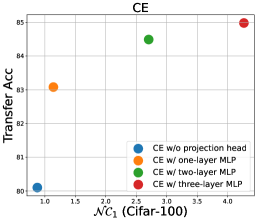
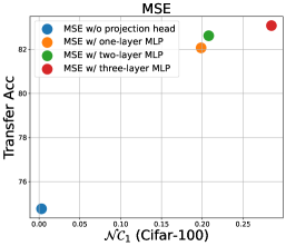
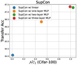
Figure 3: Trend of $\mathcal{NC}_{1}$ during training and transfer learning accuracy of the pretrained models. ResNet-50 models are pretrained using Cifar-100 dataset with CE loss (Left), MSE loss (Middle) and SupCon loss (Right). Models are pretrained with different numbers of layers for projection heads and transfered on the Cifar-10 dataset.

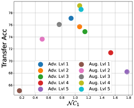
Figure 4: $\mathcal{NC}_{1}$ vs. transfer learning accuracy. Models are pre-trained on the Cifar-100 dataset with different levels of data augmentation and adversarial training strength, and then transfer accuracy of pre-trained models is reported on the Cifar-10 dataset.

Projection layers in pre-training increase feature diversity for better transferability.

The use of projection head for model pre-training was first introduced and then gained popularity in self-supervised learning [9, 27], but the reason for its effectiveness is not fully understood. In this work, we uncover its mechanism through the concept of progressive variability collapse. As we discussed in Section 2 and shown in Figure 2, the feature within-class variability collapses progressively from shallow to deep layers, with the collapse becoming more severe in deeper layers (i.e., smaller $\mathcal{NC}_{1}$ values). Based upon this discovery, our findings for model pre-training is that

The use of a projection layer in pre-training helps to prevent the variability collapse of the encoder network, thereby better preserving the information of the input data with improved transfer performance.

This can be demonstrated by our experiments in Figure 3, where we pre-train ResNet-50 models on the Cifar-100 dataset and report $\mathcal{NC}$ metrics and transfer accuracy for varying numbers of projection head layers (from one to three layers). Our results show that using projection heads significantly increases representation diversity and transfer accuracy – adding more layers of MLP projection leads to higher $\mathcal{NC}$₁ and improved transfer accuracy, although the performance improvement quickly plateaus at three layers of MLP. This suggests that the effectiveness of projection heads in model pre-training is not limited to contrastive losses but applies universally across various training loss types (e.g. CE and MSE).

Usage of the pre-trained $\mathcal{NC}$ metric for predicting transfer accuracy has limitations.

So far, we have seemingly demonstrated an universal positive correlation between the $\mathcal{NC}$₁ and transferability. However, does the increase for the $\mathcal{NC}$₁ of learned features always lead to improved model transferability? To more comprehensively characterize the relationship between $\mathcal{NC}$₁ and transferability, we pre-train ResNet50 models on the Cifar-100 dataset using different levels of data augmentations and adversarial training [63, 28, 29] strength, and then report the transfer accuracy of the pre-trained models on the Cifar-10 dataset. As shown in Figure 4, we observe that the positive relationship between the $\mathcal{NC}$₁ on the source dataset and the transfer accuracy only holds up to a certain threshold. If the $\mathcal{NC}$₁ metric is larger than a certain threshold, the transfer accuracy decreases as the $\mathcal{NC}$₁ increases.

We believe the reason behind the limitation is that the magnitude of $\mathcal{NC}_{1}$ is affected by two factors of the learned features: (i) within class feature diversity and (ii) between class discrimination. When the $\mathcal{NC}_{1}$ of is too large, the features lose the between-class discrimination, which results in poor transfer accuracy. An extreme example would be an untrained deep model with randomly initialized weights. Obviously, it possesses large $\mathcal{NC}$₁ with large feature diversity, but its features have poor between-class discrimination. Therefore, random features have poor transferability. To better predict the model transferability, we need more precise metrics for measuring both the within-class feature diversity and between-class discrimination, where the two could have a tradeoff between each other. We leave the investigation as future work.

3.2 Study of $\mathcal{NC}$ & Transfer Accuracy on Downstream Tasks

Next, we investigate the relationship between the $\mathcal{NC}$₁ metric and transfer accuracy by evaluating pre-trained models on downstream data. Transferring pre-trained large models to smaller downstream tasks has become a common practice in both the vision [12] and language [2] domains. In the meanwhile, evaluating $\mathcal{NC}$ metrics of pre-trained models on downstream data is more convenient, due to the limited availability and large size of source data. To control factors affecting our study, we freeze the whole pre-trained model without fine-tuning for each downstream task and only train a linear classifier using the downstream data. Contrary to our findings in Section 3.1 for $\mathcal{NC}$ on source data, we find that transfer accuracy is negatively correlated with the $\mathcal{NC}$₁ metric on the downstream data. This phenomenon is universal for different pre-training models and methods and holds even across different layers of the same model.

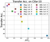
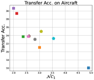
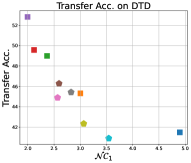
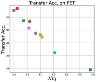
Figure 5: Transfer accuracy and $\mathcal{NC}_{1}$ of Cifar-100 pre-trained models on different downstream tasks. We pre-train ResNet50 models on Cifar-100 using different levels of data augmentation or adversarial training. Here, $\mathcal{NC}_{1}$ is measured on the downstream Cifar-10 dataset.

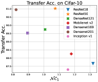
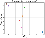
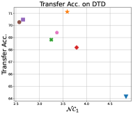
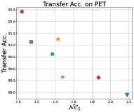
Figure 6: Transfer accuracy and $\mathcal{NC}_{1}$ of public ImageNet-1k pre-trained models on different downstream tasks. We evaluate transfer accuracy and $\mathcal{NC}_{1}$ on multiple downstream datasets using various ImageNet-1k pre-trained models, such as ResNet [34], DenseNet [35] and MobileNetV2 [36]. The $\mathcal{NC}_{1}$ is measured on the corresponding downstream dataset.

Pre-trained models with more collapsed last-layer features exhibit better transferability.

To support our claim, we pre-train various ResNet50 models on the Cifar-100 dataset using different levels of data augmentation and adversarial training intensity, similar to what we did above in Section 3.1. Once pre-trained, we evaluate the transfer accuracy of each model on four downstream datasets: Cifar-10 [30], FGVC-Aircraft [31], DTD [32] and Oxford-IIIT-Pet [33]. As shown in Figure 5, we find a negative (near linear) correlation between $\mathcal{NC}$₁ on Cifar-10 and transfer accuracy on the downstream tasks, where lower $\mathcal{NC}$₁ on Cifar-10 corresponds to higher transfer accuracy. Thus, the $\mathcal{NC}$₁ metric on Cifar-10 can serve as a reliable indicator of transfer accuracy on downstream tasks. To further reinforce our argument, we conduct experiments on the same set of downstream tasks using publicly available pre-trained models on ImageNet-1k [61], such as ResNet [34], DenseNet [35] and MobileNetV2 [36]. In Figure 6, we observe the same negative correlation between $\mathcal{NC}$₁ on the downstream data and transfer accuracy, demonstrating that this relationship is not limited to a specific training scenario or network architecture.

Moreover, this negative correlation between downstream $\mathcal{NC}_{1}$ and transfer accuracy also applies to the few-shot (FS) learning settings, as shown in Table 2 for miniImageNet and CIFAR-FS datasets. Following [65], we pre-train different models on the merged meta-training data, and then freeze the models, and learn a linear classifier at meta-testing time. During meta-testing time, support images and query images are transformed into embeddings using the fixed neural network. The linear classifier is trained on the support embeddings. On the query images, we compute the $\mathcal{NC}_{1}$ of the embeddings and record the few-shot classification accuracies using the linear model.

The contrast in the relationship between the $\mathcal{NC}$₁ metric and transfer accuracy between pre-trained data and downstream data implies distinct objectives for model pre-training and fine-tuning. On one hand, during pre-training on the source data, our goal is to generate more diverse features (large $\mathcal{NC}$₁) so that the learned features can capture the structure of the input data as explained in Section 3.1. On the other hand, for the downstream tasks, our goal is to achieve maximum between-class separation with a wide margin (small $\mathcal{NC}$₁). Furthermore, pre-trained models that have better capability in preserving structures of the input data (larger $\mathcal{NC}$₁ on the source data) tend to have wider class separation on downstream data (smaller $\mathcal{NC}$₁) and result in better transfer accuracy.

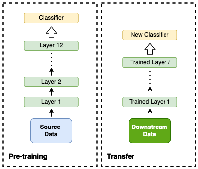
Figure 7: An illustration of layer-wise transfer learning. We use a pre-trained model up to the intermediate $i$-th layer as a feature extractor for transfer learning on the downstream tasks.

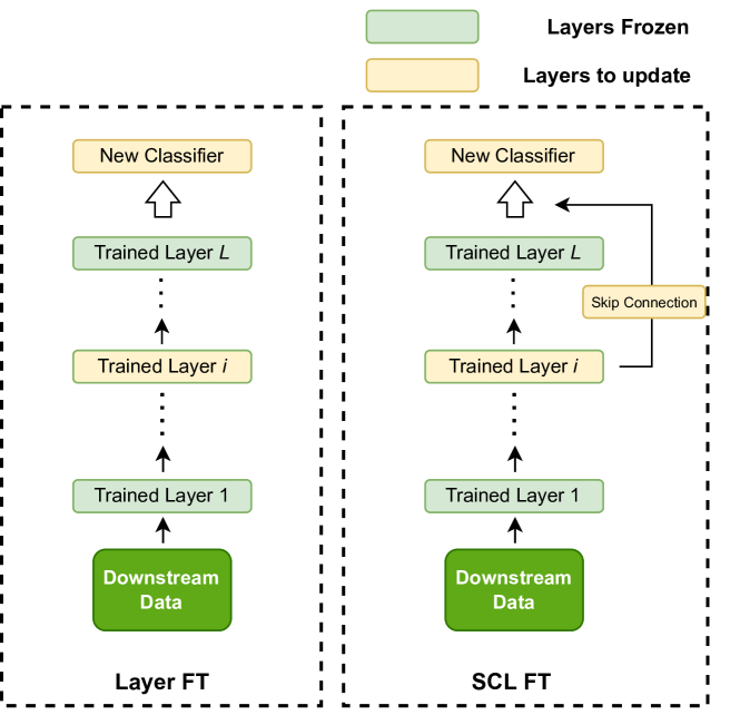
Figure 8: Illustrations of Layer FL (left) and SCL FT (right). Layer FL simply fine-tune one intermediate layer, while SCL FT adds a skip connection to the final layer.

Fewshot Accuracy
Architecture	ConvNet4		ResNet12[34]		SEResNet12[66]
	1 shot	5 shots	1 shot	5 shots	1 shot	5 shots
CIFAR-FS	61.59	77.45	68.61	82.81	69.99	83.34
miniImageNet	52.04	69.07	59.52	75.92	60.21	77.17
$\mathcal{NC}_{1}$ of models pre-trained on meta-train splits
CIFAR-FS	38.12		29.13		28.40
miniImageNet	51.82		28.24		25.58

Table 2: Average few-shot classification accuracy and $\mathcal{NC}_{1}$ metrics on CIFAR-FS and miniImageNet. The test few-shot accuracies and $\mathcal{NC}_{1}$ are evaluated on miniImageNet and tieredImageNet meta-test splits. ConvNet4 denotes a 4-layer convolutional network with 64 filters in each layer.

Layers with more collapsed output features result in better transferability.

In addition, the correlation between the $\mathcal{NC}$₁ metric and transfer accuracy that we observed is not limited to different pre-trained models, but also occurs across different layers of the same pre-trained model. Specifically, as depicted in Figure 7, we use the output of each individual layer as a "feature extractor" and assess its transfer accuracy by training a linear classifier on top of it. Surprisingly, regardless of the layer’s depth, if the layer’s outputs are more collapsed (smaller $\mathcal{NC}$₁), the resulting features lead to better transfer accuracy. To support our claim, we carried out experiments using the ImageNet-1k pre-trained ResNet34 model [61, 34]. We evaluated the $\mathcal{NC}_{1}$ metric on each residual block’s output feature for the downstream data, as shown in Figure 9 (a). The results indicate that the output features with a smaller $\mathcal{NC}_{1}$ lead to better transfer accuracy, and there is a near-linear relationship between $\mathcal{NC}_{1}$ and transfer accuracy, suggesting that transfer accuracy is more closely related to the degree of variability collapse in the layer than the layer’s depth. This phenomenon is observed across different network architectures. Figure 9 (b) shows similar results with experiments on the ViT-B (vision transformer base model) [12] using a pre-trained checkpoint available online.

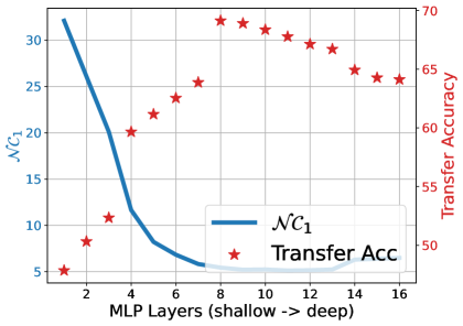
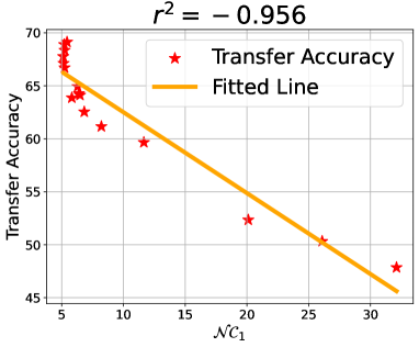
(a) ResNet34

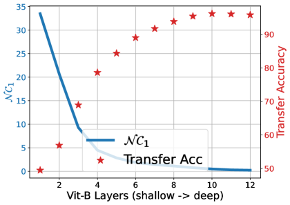
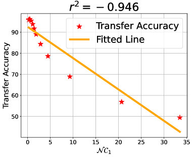
(b) ViT-B

Figure 9: $\mathcal{NC}_{1}$ and transfer learning accuracy of different layers from a pre-trained model (Left) and nearly linear relationship between transfer learning accuracy and $\mathcal{NC}_{1}$ (Right). We use (a) an ImageNet-1k dataset pre-trained ResNet34 model and (b) a released pre-trained ViT-B model. We use the Cifar-10 dataset for transfer learning and measuring the corresponding $\mathcal{NC}_{1}$.

3.3 A Simple & Efficient Fine-tuning Strategy for Improving Transferability

Finally, we show that the relationship we discovered between layer variability and transfer accuracy in Section 3.2 can be used to design simple and effective fine-tuning strategies. There are two common transfer learning approaches for vision tasks: (i) fixed feature training [8, 7, 29], which uses the pre-trained model up to the penultimate layer as a feature extractor and trains a new linear classifier on top of the features for the downstream task, and (ii) full model fine-tuning [12, 4, 28], which fine-tunes the entire pre-trained model to fit the downstream task. While full fine-tuning can be computationally expensive, fixed feature training often results in lower performance. An alternative approach, selective layer fine-tuning, has the potential to achieve better transfer accuracy but has received less attention [67, 68]. Based on the correlation between penultimate layer variability and transfer accuracy, we conjecture that

The optimal transfer accuracy can be achieved by selectively fine-tuning layers to make the penultimate layer’s features as collapsed as possible for the downstream training data.

We propose two simple fine-tuning strategies to increase the level of collapse in the penultimate layer, and we report the results in Table 3. Our results indicate that the proposed methods achieve comparable or even better transfer accuracy compared to full model fine-tuning. In the following, we describe our proposed fine-tuning methods in detail.

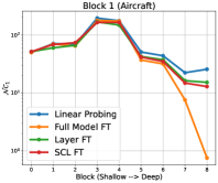
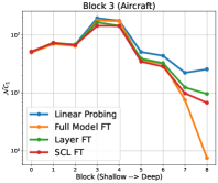
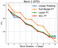
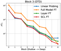
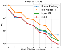
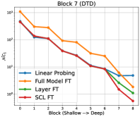
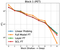
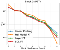
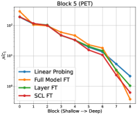
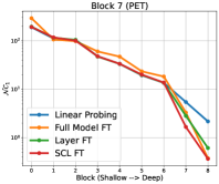
Figure 10: Layer-wise $\mathcal{NC}_{1}$ for different fine-tuning methods. We compare the layer-wise $\mathcal{NC}_{1}$ across different fine-tuning methods, including linear probing, Layer FT, and SCL FT, using the ImageNet-1k pre-trained ResNet18 backbone. We evaluate the models on the downstream datasets of FGVC-Aircraft (top), DTD (middle), and Oxford-IIIT-Pet (bottom). For the figures from left to right, we plot the results of fine-tuning only Block 1, Block 3, Block 5, and Block 7 in both Layer FT and SCL FT.

• Layer fine-tuning (FT). First, we show that we can collapse features of the penultimate layer simply by fine-tuning only one of the intermediate layers, while keeping the rest of the network frozen. As shown in Figure 10, fine-tuning the layer closer to the final layer usually leads to more collapsed features of the penultimate and, thus, the better transfer accuracy. This is because the information from the inputs has been better extracted and distilled as getting closer to final layers. On the other hand, it is a common scenario in deep networks that the closer a layer is to the final layer, the more parameters it has . Therefore, to achieve a better transfer performance while at the same time maintaining parameter efficiency, we choose to fine-tune one of the middle layers . As shown in Table 3, with only $6\%-8\%$ parameters fine-tuned, this simple Layer FT approach leads to substantial performance gains compared to vanilla linear probing (i.e., fixed feature training) on a variety of datasets, including Cifar, FGVC-Aircraft [31], DTD [32], and Oxford-IIIT-Pet [33]. This approach works well for both ResNet and ViT network architectures.

• Skip connection layer (SCL) fine-tuning (FT). Based on the Layer FT approach, we can further enhance the method by introducing a skip connection from the fine-tuned layer to the penultimate layer; see Figure 8 (right) for an illustration. Then, we can use the combined features (i.e., addition of two outputs) of these two layers as the new feature for training the linear classifier and fine-tuning the selected layer. Similar to Layer FT, although fine-tuning the layer closer to the final layer usually leads to more collapsed features of the penultimate and the better transfer accuracy(see Figure 10), fine-tuning one of the middle layers is sufficient to yield satisfactory results. The proposed SCL FT method allows the network to fine-tune the selected layer more effectively by explicitly passing the data’s information from the intermediate layer to the classifier, without losing information through the cascade of intermediate layers. Furthermore, the approach takes advantage of the depth of the deep models, making sure the more distilled features from the penultimate layer can also be passed to the linear classifier. According to Table 3, SCL FT outperforms Layer FT and achieves comparable or better results than full model FT on various datasets for both ResNet and ViT network architectures.

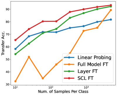
Figure 11: Transfer accuracy for different fine-tuning methods with varying size of downstream training dataset. We fine-tune ResNet18 models pre-trained on ImageNet-1k using subsets of the Cifar-10 downstream dataset with varying sizes.

Significantly improved memory efficiency and reduced overfitting compared to full FT.

Full model FT involves retraining all 23 million parameters for ResNet50 or 88 million parameters for ViT-B32. In contrast, our methods, Layer FT and SCL FT, are much more efficient as they can achieve on-par or even better results by fine-tuning only around 8% of the model’s parameters, as shown in tables Tables 5, 6 and 7. These methods can achieve equal or better performance compared to full model FT while being less prone to overfitting. In the case of limited data, fine-tuning the entire model on the downstream training data can result in severe overfitting and hence poor generalization performance. In contrast, because our methods only fine-tune a small portion of the parameters, they are more robust to data scarcity with reduced overfitting. To demonstrate this, we fine-tuned pre-trained models on different size of subsets of Cifar-10 training samples and report the results in Figure 11. Our results show that full model FT is vulnerable to data scarcity and performs worse than linear probing when the size of downstream training data is limited. In contrast, our layer FT and SCL FT remain robust and outperform full model FT until a large amount of downstream training data is available.

Backbone	ResNet18					ResNet50					ViT-B
Dataset	Cifar-10	Cifar-100	Aircraft	DTD	PET	Cifar-10	Cifar-100	Aircraft	DTD	PET	Aircraft	DTD	PET
Transfer accuracy
Linear Probe	81.64	59.75	38.94	60.16	86.26	85.33	65.47	43.23	68.46	89.26	43.65	73.88	92.23
Layer FT	92.12	74.24	67.36	66.01	87.90	94.04	77.47	70.27	67.66	89.40	65.83	77.13	92.94
SCL FT	93.11	74.35	69.19	69.84	89.78	94.94	78.32	70.72	72.87	91.69	65.80	77.34	93.13
Full Model FT	92.11	78.65	78.25	41.38	74.24	85.51	78.88	80.77	38.83	73.24	64.66	76.54	93.02
$\mathcal{NC}_{1}$ evaluated on the penultimate layer feature $\bm{h}^{L-1}$
Linear Probe	1.82	22.72	22.50	4.51	2.32	1.84	18.36	20.36	3.52	1.45	17.91	1.99	0.66
Layer FT	0.32	4.82	5.80	1.80	1.05	0.28	3.22	3.37	1.68	0.68	6.98	1.62	0.44
SCL FT	0.27	3.25	1.78	0.94	0.63	0.22	2.61	1.02	0.64	0.39	7.48	1.33	0.35
Full Model FT	0.08	0.39	0.75	1.83	0.38	0.17	0.15	0.61	1.85	0.28	3.78	1.11	0.21
Percentage of parameters fine-tuned
Linear Probe	0.05%	0.46%	0.46%	0.22%	0.17%	0.09%	0.86%	0.86%	0.41%	0.32%	0.09%	0.04%	0.03%
Layer FT	8.27%	8.64%	8.64%	8.42%	8.38%	6.52%	7.24%	7.24%	6.82%	6.73%	8.18%	8.14%	8.13%
SCL FT	8.27%	8.64%	8.64%	8.42%	8.38%	6.52%	7.24%	7.24%	6.82%	6.73%	8.18%	8.14%	8.13%
Full Model FT	100%	100%	100%	100%	100%	100%	100%	100%	100%	100%	100%	100%	100%

Table 3: Transfer learning results for Linear probing, layer fine-tuning, SCL fine-tuning and full model fine-tuning on various downstream datasets. We use public ResNet models pre-trained on ImageNet-1k [61], and ViT-B model pre-trained on JFT [64] and ImageNet-21k [69] datasets.

4 Discussion & Conclusion

In this work, we have explored the relationship between the degree of feature collapse, as measured by the $\mathcal{NC}$, and transferability in transfer learning. Our findings show that there is a twofold relationship between $\mathcal{NC}$ and transferability: (i) models that are less collapsed on the source data have better transferability up to a certain threshold; and (ii) more collapsed features on the downstream data leads to better transfer performance. This relationship holds both across and within models. Based on these findings, we propose a simple yet effective model fine-tuning method with significantly reduced number of fine-tuning parameters. Our experiments show that our proposed method can achieve comparable or even superior performance compared to full model FT across various tasks and setups. Our findings open up new avenues for future research that we discuss in the following.

Neuron collapse is not a pure training phenomenon.

Previous work [43] points out that $\mathcal{NC}$ is mainly an optimization phenomenon that does not necessarily relate to generalization (or transferability). Our work, on one hand, corroborates with the finding that pretraining $\mathcal{NC}$ does not always suggest better transferability, but also shows a positive correlation between pretraining $\mathcal{NC}$ and transferability to a certain extent. On the other hand, our work also shows that downstream $\mathcal{NC}$ on a dataset where $\mathcal{NC}$ is well-defined correlates with the transfer performances across different datasets and thus could be a general indicator for the transferability. This suggests that $\mathcal{NC}$ may not be merely an optimization phenomenon. An important future direction we will pursue is to theoretically understand the connection between transferability and $\mathcal{NC}$.

Boost model transferability by insights from $\mathcal{NC}$.

Our findings can be leveraged to enhance model transferability from two perspectives. Firstly, the correlation between pretraining $\mathcal{NC}$ and transferability suggests that increasing $\mathcal{NC}_{1}$ to a certain extent can boost transferability, which can be accomplished through popular methods like multi-layer projection heads and data augmentation. We expect that other methods that focus on the geometry of the representations could also be developed. Secondly, by showing the strong correlation between downstream $\mathcal{NC}$ and transfer accuracy, we can devise simple but effective strategies for efficient transfer learning. Although our simple approach may not be the optimal way to take advantage of this relationship, we believe that there are more potent methods that could exploit this relationship better and therefore lead to better transferability. We leave this as a topic for future investigation.

Transfer learning beyond $\mathcal{NC}$.

Our results indicate that $\mathcal{NC}$ on the source datasets is related to transferability to a certain extent. However, identifying the threshold and explaining the change in transferability beyond this threshold is challenging using the $\mathcal{NC}$ framework alone. Moreover, solely relying on $\mathcal{NC}$ to study transfer learning may not always be appropriate. For instance, recent research [55] demonstrated that representations learned through unsupervised contrastive methods are uniform across hyperspheres, and [70] showed that representations learned using the principle of maximal coding rate reduction (MCR²) form subspaces rather than collapse to single points. Therefore, further disclosing the mysteries shrouded around transfer learning would require new frameworks and new tools, which we leave for future investigation.

The appendices are organized as follows. In Appendix A, we review other metrics that measure feature diversity and discrimination. In Appendix B, we provide experimental details for each figure and each table in the main body of the paper. Finally, in Appendix C, we provide complimentary experimental results for Section 3.2, and the proposed fine-tuning methods in Section 3.3.

Appendix A Other Metrics for Measuring $\mathcal{NC}$

Numerical rank of the features $\bm{H}$.

The $\mathcal{NC}$₁ does not directly reveal the dimensionality of the features spanned for each class. In this case, measuring the rank of the features ($\bm{H}_{k}$) is more suitable. However, the calculations for both $\mathcal{NC}$₁ and rank are expensive when feature dimension gets too large. Thus, we emphasize introducing numerical rank [71] as an approximation.

$$\widetilde{\operatorname{rank}}(\bm{H})\;:=\;\frac{1}{K}\sum_{k=1}^{K}\left\|\bm{H}_{k}\right\|_{F}^{2}/\left\|\bm{H}_{k}\right\|_{2}^{2},$$

where $\left\|\cdot\right\|_{F}$ represents the Frobenius norm and $\left\|\cdot\right\|_{2}$ represents the Spectral norm. $\widetilde{\operatorname{rank}}(\bm{H})$(numerical rank) could be seen as an estimation of the true rank for any matrix. Note that we use the Power Method to approximate the Spectral norm. The metric is evaluated by averaging over all classes, and a smaller $\widetilde{\operatorname{rank}}(\bm{H})$ indicates more feature collapse towards their respective class means.

Class-distance normalized variance (CDNV) [42].

To alleviate the computational issue of $\mathcal{NC}_{1}$, the class-distance normalized variance (CDNV) introduced in [42] provides an alternative metric that is inexpensive to evaluate. Let $\mathcal{X}$ denote the space of the input data $\bm{x}$, and let $\bm{Q}_{k}$ be the distribution over $\mathcal{X}$ conditioned on class $k$. For two different classes with $\bm{Q}_{i}$ and $\bm{Q}_{j}$ ($i\not=j$), the CDNV metric can be described by the following equation:

$$V_{\phi_{\bm{\theta}}}(\bm{Q}_{i},\bm{Q}_{j})=\frac{\text{Var}_{\phi_{\bm{\theta}}}(\bm{Q}_{i})+\text{Var}_{\phi_{\bm{\theta}}}(\bm{Q}_{j})}{2||\mu_{\phi_{\bm{\theta}}}(\bm{Q}_{i})-\mu_{\phi_{\bm{\theta}}}(\bm{Q}_{j})||_{2}^{2}},$$

where $\mu_{\phi_{\bm{\theta}}}(\bm{Q}_{k})=\mathbb{E}_{\bm{x}\sim\bm{Q}_{k}}[\phi_{\bm{\theta}}(\bm{x})]$ denotes the class-conditional feature mean and $\text{Var}_{\phi_{\bm{\theta}}}(\bm{Q}_{k})=\mathbb{E}_{\bm{x}\sim\bm{Q}_{k}}[||\phi_{\bm{\theta}}(\bm{x})-\mu_{\phi_{\bm{\theta}}}(\bm{Q}_{k})||^{2}]$ denotes the feature variance for the distribution $\bm{Q}_{k}$. Although the exact expectation is impossible to evaluate, we can approximate it via its empirical mean and empirical variance on the given training samples as

$$\widehat{V}_{\phi_{\bm{\theta}}}(\bm{Q}_{i},\bm{Q}_{j})\;=\;\frac{\widehat{\text{Var}}_{\phi_{\bm{\theta}}}(\bm{Q}_{i})+\widehat{\text{Var}}_{\phi_{\bm{\theta}}}(\bm{Q}_{j})}{2||\widehat{\mu}_{\phi_{\bm{\theta}}}(\bm{Q}_{i})-\widehat{\mu}_{\phi_{\bm{\theta}}}(\bm{Q}_{j})||^{2}},$$

$$\widehat{\mu}_{\phi_{\bm{\theta}}}(\bm{Q}_{k})\;=\;\frac{1}{n_{k}}\sum_{i=1}^{n_{k}}\phi_{\bm{\theta}}(\bm{x}_{k,i}),\;\widehat{\text{Var}}_{\phi_{\bm{\theta}}}(\bm{Q}_{k})\;=\;\frac{1}{n_{k}}\sum_{i=1}^{n_{k}}||\phi_{\bm{\theta}}(\bm{x}_{k,i})-\mu_{\phi_{\bm{\theta}}}(\bm{X}_{k})||^{2}.$$

To characterize the overall degree of collapse for a model, we can use the empirical CDNV between all pairwise classes (i.e., $\text{Avg}_{i\neq j}[\widehat{V}_{\phi_{\bm{\theta}}}(\bm{Q}_{i},\bm{Q}_{j})]$). If a model achieves perfect collapse on the data, we have $\text{Avg}_{i\neq j}[\widehat{V}_{\phi_{\bm{\theta}}}(\bm{Q}_{i},\bm{Q}_{j})]=0$. Because the CDNV metric is purely norm-based, computational complexity scales linearly with the feature dimension $d$, making it a good surrogate for $\mathcal{NC}_{1}$ when the feature dimension $d$ is large.

Appendix B Extra Experimental Details

In this section, we provide additional technical details for all the experiments in the main body of the paper to facilitate reproducibility. In particular, Appendix B.1 includes all the experimental details for the figures (from Figure 2 to Figure 11), and Appendix B.2 includes all the experimental details for the tables (from Table 1 to Table 3).

General experiment setups.

We perform all experiments using a single NVIDIA A40 GPU. Unless otherwise specified, all pre-training and transfer learning are run for 200 epochs using SGD with a momentum of 0.9, a weight decay of $1\times 10^{-4}$, and a dynamically changing learning rate ranging from $1\times 10^{-1}$ to $1\times 10^{-4}$ controlled by a CosineAnnealing learning rate scheduler as described in [72]. When using ImageNet pre-trained models, we resize each input image to $224\times 224$ for training, testing, and evaluating $\mathcal{NC}$.

B.1 Technical Detail for the Figures

Experimental details for Figure 2.

For MNIST [60] and FashionMNIST [62], we train MLP models consisting of 9 layers with a fixed hidden dimension of 784 across all layers. This choice aligns the hidden dimension with the input data dimension. We train these models for 150 epochs. For CIFAR-10 and CIFAR-100 [30], we employ the widely used ResNet18 [34] architecture and train the models for 200 epochs. After pre-training, we calculate the layer-wise $\mathcal{NC}_{1}$ on the corresponding training datasets and plot the trend of $\mathcal{NC}_{1}$ vs. layers.

Experimental details for Figure 3.

In Figure 3, we pre-train ResNet50 models with different number of projection layers and different loss functions (CE, MSE, SupCon) using Cifar-100 for 200 epochs. Then we use the learned model to do transfer learning on Cifar-10. The $\mathcal{N}C_{1}$ is then evaluated on the source dataset. For projection head used for different losses, we use MLP with ReLU activation, and we vary the number of its layers.

Experimental details for Figure 4.

In Figure 4, we pre-train ResNet50 models using different levels of data augmentation and adversarial training. For data augmentation, we consider RandomCrop, RandomHorizontalFlip, ColorJitter, and RandomGrayScale. We increase the levels of data augmentation by adding one additional type of augmentation to the previous level. For Level 1, we only do the standardization for samples to make the values have mean $0$, variance $1$; for level 2, we add RandomCrop to the Level 1 augmentation; for level 3, we add RandomHorizontalFlip to the previous level, and so on, so forth. Previous research has demonstrated the effectiveness of adversarial pre-training for enhancing transferability [28, 29]. To investigate the impact of adversarial training with more detail, we adopted the $\ell_{\infty}$-norm bounded adversarial training framework proposed in [63], employing five different levels of attack sizes: $\frac{1}{255}$, $\frac{2}{255}$, $\frac{3}{255}$, $\frac{5}{255}$, and $\frac{8}{255}$. Our experimental results, illustrated in Figure Figure 4, confirm that using smaller attack sizes in adversarial training can enhance the transferability of pre-trained models, while larger step sizes can negatively impact the transferability.

Experimental details for Figure 5 and Figure 6.

With the same pre-training setup as in Figure 4, we transfer the pre-trained models to four different downstream datasets: Cifar-10, FGVC-Aircraft, DTD, and Oxford-IIIT-Pet. Although there are many other benchmark datasets to use, we choose these four because the number of samples for each class is balanced for the ease of study. This aligns with the scenario where $\mathcal{NC}$ is studied in [16]. In Figure 5, we pre-train ResNet50 models on Cifar-100 dataset, while in Figure 6 we conduct similar experiments using public avaiable pre-trained models on ImageNet-1k [61] including ResNet [34], DenseNet [35], and Mobilenet-v2 [36]

Experimental details for Figure 9.

In Figure 9 (a), we used a pre-trained ResNet34 [34] model trained on ImageNet-1k [61]. To simplify the computation of $\mathcal{NC}_{1}$, we extracted the output from each residual block as features (as demonstrated in Figure 12), and then conducted adaptive average pooling on these features, ensuring that each channel contained only one element. We then computed $\mathcal{NC}_{1}$ and performed transfer learning on the resulting features. In Figure 9 (b), we used a pre-trained Vit-B32 [12] model that is publicly available online. For each encoder layer $l$ in Vit-B32, the output features $\bm{h}_{l}$ are of dimension 145 (which includes the number of patches plus an additional classification token) $\times$ 768 (the hidden dimension), i.e., $\bm{h}_{l}\in\mathbb{R}^{145\times 768}$. To conduct our layer-wise transfer learning experiment, we first applied average pooling to the 145 patches to reduce the dimensionality of the feature vectors. Specifically, we used an average pooling operator $\textit{ap}:\mathbb{R}^{145\times 768}\mapsto\mathbb{R}^{768}$ to downsample $\bm{h}_{l}$, resulting in $\widehat{\bm{h}_{l}}=\textit{ap}(\bm{h}_{l})$. Subsequently, we trained a linear classifier using the downsampled features $\widehat{\bm{h}_{l}}$ on top of each encoder layer.

Experimental details for Figure 10.

In Figure 10, we investigate the effects of different fine-tuning methods on the layerwise $\mathcal{NC}_{1}$ when we are fine-tuning ResNet18 models pre-trained on ImageNet-1k. To facilitate the computation of $\mathcal{NC}_{1}$, we adopt the same adaptive pooling strategy as in Figure 9 on the features from each residual block of the ResNet model.

Experimental details for Figure 11.

We empirically demonstrate that our proposed Layer FT and SCL FT are more robust to data scarcity compared with linear probing and full model FT. To this end, we transfer the ImageNet-1k pre-trained ResNet18 model on subsets of Cifar-10 with varying sizes. More specifically, we select the sizes from a logarithmically spaced list of values: [10, 24, 59, 142, 344, 835, 2022, 4898]. We note that when fine-tuning the models using Layer FT and SCL FT, in particular, we only fine-tune Block 5 of the pre-trained ResNet18 model.

B.2 Technical Detail for the Tables

Experimental details for Table 1.

In Table 1, we pre-trained ResNet18 models on the Cifar-100 dataset using three different loss functions: CE, MSE, and SupCon, each for 200 epochs. For transfer to the Cifar-10 dataset, we froze the pre-trained models and trained only a linear classifier on top of them for 200 epochs. Both procedures employed the cosine learning rate scheduler with an initial learning rate of $0.1$. We computed $\mathcal{N}C_{1}$ on the source dataset (Cifar-100) and evaluated the downstream dataset’s (Cifar-10) test accuracy.

Experimental details for Table 2.

The negative correlation between downstream $\mathcal{NC}_{1}$ and transfer accuracy extends to few-shot learning, as shown in Table 2. We observed that the $\mathcal{NC}_{1}$ of the penultimate layer negatively correlates with the few-shot classification accuracies on miniImageNet and CIFAR-FS meta-test splits. To obtain few-shot accuracy, we followed [65] and first learned a feature extractor through supervised learning on the meta-training set. We then trained a linear classifier on top of the representations obtained by the extractor. We calculated the $\mathcal{NC}_{1}$ of the penultimate layer in the feature extractor network using different architectures and observed that they are negatively correlated with the 1-shot and 5-shot accuracies.

Following previous works [73, 74], ResNet12 is adopted as our backbone: the network consists of 4 residual blocks, where each has three convolutional layers with $3\times 3$ kernel; a $2\times 2$ max-pooling layer is applied after each of the first three blocks; a global average-pooling layer is on top of the fourth block to generate the feature embedding.

On the optimization side, we use SGD optimizer with a momentum of $0.9$ and a weight decay of $5e-4$. Each batch consists of 64 samples. The learning rate is initialized as $0.05$ and decayed with a factor of $0.1$ by three times for all datasets, except for miniImageNet where we only decay twice as the third decay has no effect. We train 100 epochs for miniImageNet, and $90$ epochs for both CIFAR-FS. When training the embedding network on transformed meta-training set, we adopt augmentations such as random crop, color jittering, and random horizontal flip as in [75]. For meta-testing time, we train a softmax regression base classifier. We use the multi-class logistic regression implemented in scikitlearn [76] for the base classifier.

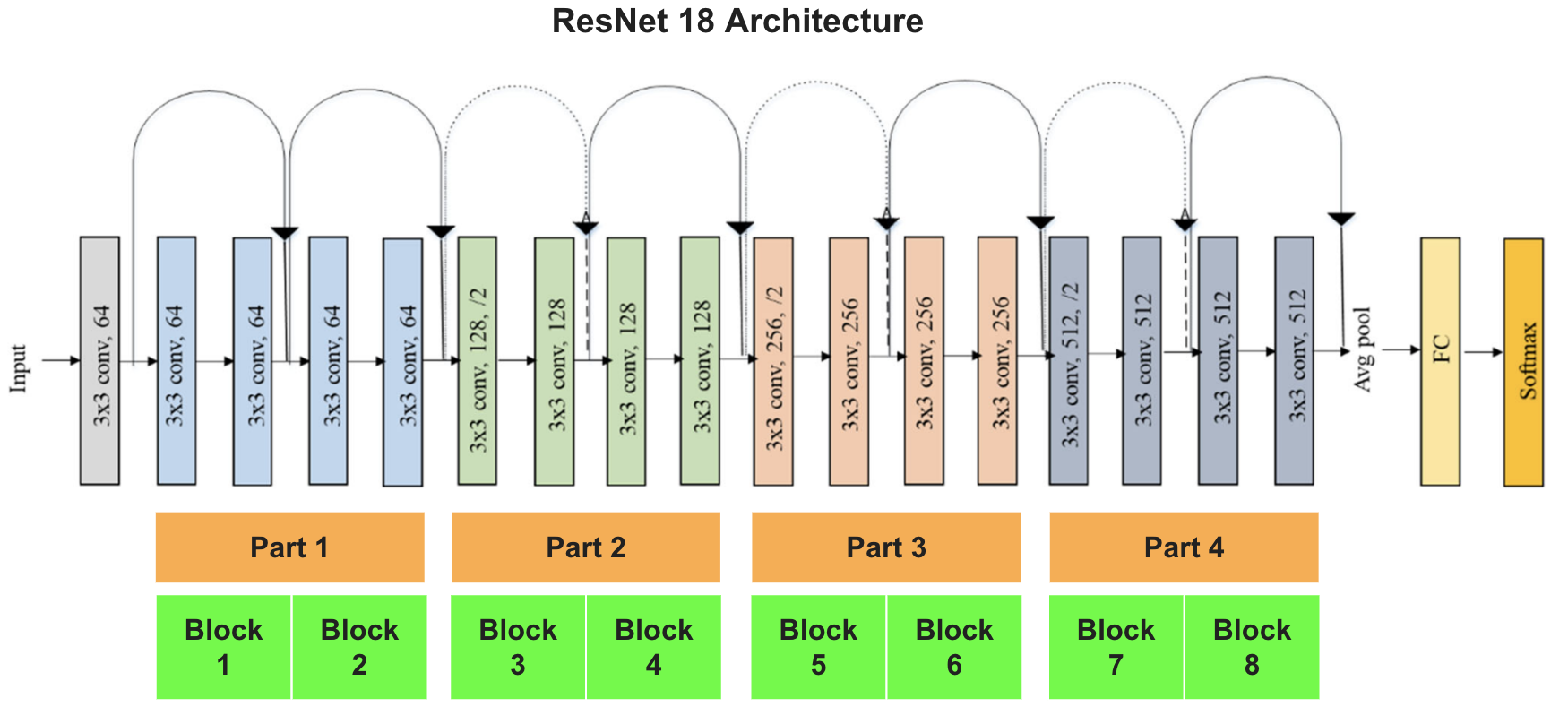
Figure 12: Fine-tuning unit of ResNet. Image of ResNet18 from [77].

Experimental details for Table 3.

In Table 3, we compare the performance between linear probing, Layer FT, SCL FT and full model FT based upon a wide variety of experimental setups, such as different model architectures, different pre-training and downstream datasets. In particular, we consider the following.

• Fine-tuning blocks for different network architectures. Each residual block in the ResNet models is regarded as a fine-tuning unit, and only the first residual block of each channel dimension is fine-tuned. As illustrated in Figure 12, the feature extractor of ResNet18 is partitioned into four parts, with each part containing two residual blocks of the same channel dimension, and the first block of each part is fine-tuned. In the case of the Vit-B32 model, each of its 12 encoder layers is considered a fine-tuning unit.

• SCF FT for different models. For SCL FT with skip connections, the Vit-B32 model had a constant feature dimension across layers, making it easy to directly apply the skip connection between the fine-tuned layer and the penultimate layer features. However, ResNet models have varying numbers of channels and feature dimensions across layers, making it necessary to calculate the skip connection differently. To address this for ResNet, we first perform adaptive average pooling on the fine-tuned layer features to ensure that each channel had only one entry, and then we use zero-padding to match the number of channels with the penultimate layer features. Finally, for both ResNet and ViT models, we apply the skip connection and used the combined features to train the classifier.

• Batch normalization. For a fair comparison between different fine-tuning methods, we always let the normalization layers [58, 78] update the running means and variances on the downstream data for all fine-tuning methods (i.e., linear probing, layer FT, SCL FT, and full model FT).

Appendix C Additional Experimental Results

In this final part of the appendices, we present extra complementary experimental results to corroborate our claims in the main body of the paper.

C.1 Experiments for Section 3.2 & Section 3.3

Extra experiments for Section 3.2.

In the main paper’s Figure 5, we illustrate a correlation between $\mathcal{NC}_{1}$ on Cifar-10 and transfer accuracy on various downstream tasks for ResNet50 models pre-trained on Cifar100. However, when evaluating this relationship directly on downstream datasets for ResNet50 models pre-trained on Cifar100, the negative correlation becomes less apparent, as depicted in Figure 13. Nonetheless, we believe that $\mathcal{NC}_{1}$ is somewhat less sensitive when the magnitude is too large, as shown in Figure 6; when $\mathcal{NC}_{1}$ has a smaller magnitude, the negative correlation on downstream data becomes clear again.

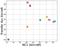
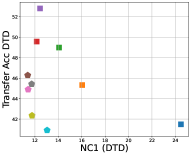
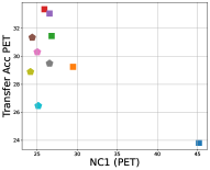
Figure 13: Transfer accuracy on different downstream tasks and $\mathcal{NC}_{1}$. Transfer accuracy and $\mathcal{NC}_{1}$ are measured on the same downstream datasets.

Extra experiments for Section 3.3.

In Figure 10, we only visualized the layer-wise $\mathcal{NC}_{1}$ for ResNet18 models on downstream datasets with different fine-tuning method. Here, for a more comprehensive study, we conducted similar experiments for the pre-trained ViT-B32 models, where we use the classification token of each layer to calculate the associate $\mathcal{NC}_{1}$. In Figure 14, we observe a similar trend that we have seen on ResNet18 models, that within-class variability of the ViT model (measured by $\mathcal{NC}_{1}$) decreases from shallow to deep layers and the minimum values often appear near the penultimate layers. Moreover, we can observe that Layer FT and SCL FT always have smaller penultimate $\mathcal{NC}_{1}$ compared with Linear Probing and also better transfer performance.

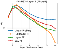
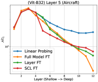
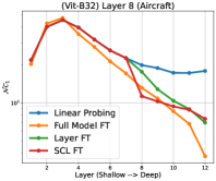
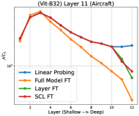
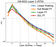
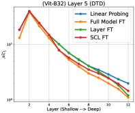
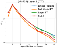
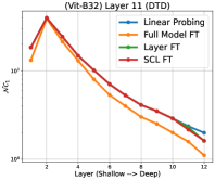
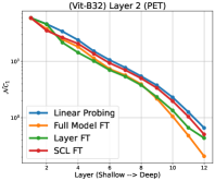
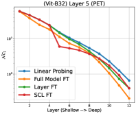
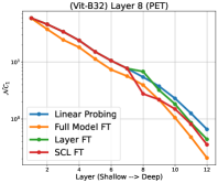
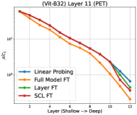
Figure 14: Layer-wise $\mathcal{NC}_{1}$ for different fine-tuning methods. We compare the layer-wise $\mathcal{NC}_{1}$ across different fine-tuning methods, including linear probing, Layer FT, and SCL FT, using the pre-trained Vit-B32 model. We evaluate the models on the downstream datasets of FGVC-Aircraft (top), DTD (middle), and Oxford-IIIT-Pet (bottom). For the figures from left to right, we plot the results of fine-tuning only Layer 2, Layer 5, Layer 8, and Layer 11 in both Layer FT and SCL FT.

C.2 Extra Experimental Results for Efficient Fine-Tuning in Section 3.3

In Table 3, to maintain a balance between good transfer learning performance and parameter efficiency, we have presented the fine-tuning results of SCL FT and Layer FT for the middle block/layer (i.e., Block 5 for ResNet18, Block 8 for ResNet50 and Layer 8 for Vit-B32). In this section, we first report the optimal transfer accuracy that can be achieved by Layer FT and SCL FT in Table 4. The best results are typically achieved by fine-tuning layers near the penultimate layer due to better extracted and distilled features. Moreover, we conduct a comprehensive ablation study by fine-tuning more individual layers for SCL FT and Layer FT of pre-trained ResNet18, ResNet50, and Vit-B32 models. We then show the corresponding transfer accuracy and percentage of parameters fine-tuned for ResNet18, ResNet50, and Vit-B32 in Tables 5, 6 and 7, respectively. From these tables, we observe that fine-tuning the layer or block near the penultimate layer consistently leads to the best transfer accuracy for SCL FT and Layer FT.

However, we note that the trend of achieving better transfer accuracy with smaller penultimate layer $\mathcal{NC}$₁ is not always consistent in terms of model fine-tuning. For instance, in Table 5, the fine-tuned model with the smallest penultimate layer $\mathcal{NC}$₁ does not yield the best transfer accuracy for the Cifar-10 dataset. We attribute this to overfitting. When the downstream dataset is small, fine-tuning to achieve the smallest penultimate layer $\mathcal{NC}$₁ can cause overfitting, leading to degraded transfer accuracy. Our experiments in Table 3 and recent studies such as [43] support this claim.

Backbone	ResNet18					ResNet50					ViT-B
Dataset	Cifar-10	Cifar-100	Aircraft	DTD	PET	Cifar-10	Cifar-100	Aircraft	DTD	PET	Aircraft	DTD	PET
Transfer accuracy
Linear Probe	81.64	59.75	38.94	60.16	86.26	85.33	65.47	43.23	68.46	89.26	43.65	73.88	92.23
Layer FT	93.08	75.04	68.65	68.56	88.01	94.04	77.82	72.67	71.81	90.13	65.83	77.13	93.02
SCL FT	93.65	75.69	70.24	71.22	89.78	94.94	78.40	74.26	74.89	91.71	65.80	77.34	93.19
Full Model FT	92.11	78.65	78.25	41.38	74.24	85.51	78.88	80.77	38.83	73.24	64.66	76.54	93.02
$\mathcal{NC}_{1}$ evaluated on the penultimate layer feature $\bm{h}^{L-1}$
Linear Probe	1.82	22.72	22.50	4.51	2.32	1.84	18.36	20.36	3.52	1.45	17.91	1.99	0.66
Layer FT	0.22	1.60	2.47	1.10	1.49	0.28	7.72	1.27	0.78	0.32	6.98	1.62	0.44
SCL FT	0.16	1.43	1.43	0.56	0.63	0.22	7.24	0.37	0.51	0.16	7.48	1.33	0.40
Full Model FT	0.08	0.39	0.75	1.83	0.38	0.17	0.15	0.61	1.85	0.28	3.78	1.11	0.21
Percentage of parameters fine-tuned
Linear Probe	0.05%	0.46%	0.46%	0.22%	0.17%	0.09%	0.86%	0.86%	0.41%	0.32%	0.09%	0.04%	0.03%
Layer FT	32.90%	33.17%	33.17%	33.01%	2.23%	6.52%	1.18%	26.33%	25.99%	25.93%	8.18%	8.14%	8.13%
SCL FT	32.90%	33.17%	33.17%	33.01%	8.38%	6.52%	1.18%	26.33%	25.99%	25.93%	8.18%	8.14%	8.13%
Full Model FT	100%	100%	100%	100%	100%	100%	100%	100%	100%	100%	100%	100%	100%

Table 4: Comparison between optimal transfer learning results for layer fine-tuning, SCL fine-tuning, Linear probing and full model fine-tuning on various downstream datasets. We use public ResNet models pre-trained on ImageNet-1k [61], and ViT-B model pre-trained on JFT [64] and ImageNet-21k [69] datasets.

Transfer Accuracy
FT method	Linear Probe	Block 1		Block 3		Block 5		Block 7		Full Model
		Layer FT	SCL FT	Layer FT	SCL FT	Layer FT	SCL FT	Layer FT	SCL FT
Cifar-10	81.64	91.23	91.76	92.02	92.43	92.12	93.11	93.08	93.65	92.11
Cifar-100	59.75	73.36	75.04	73.87	74.41	74.24	74.35	75.04	75.69	78.65
Aircraft	38.94	55.06	56.86	60.49	61.54	67.36	69.19	68.65	70.24	78.25
DTD	60.16	60.00	62.07	61.70	65.11	66.01	69.84	68.56	71.22	41.38
PET	86.26	86.67	88.14	88.01	89.02	87.90	89.78	86.56	89.18	74.24
$\mathcal{NC}_{1}$ evaluated on the penultimate layer feature $\bm{h}^{L-1}$
Cifar-10	1.82	0.72	0.64	0.51	0.41	0.32	0.27	0.22	0.16	0.08
Cifar-100	22.72	10.50	9.74	7.18	7.16	4.82	3.25	1.60	1.43	0.39
Aircraft	22.50	14.64	12.28	8.30	5.02	5.80	1.78	2.47	1.43	0.75
DTD	4.51	4.05	3.20	2.85	1.82	1.80	0.94	1.10	0.56	1.83
PET	2.32	2.00	1.56	1.49	1.08	1.05	0.63	0.61	0.37	0.38
Percentage of parameters fine-tuned
	0.23%	0.89%		2.28%		8.43%		33.02%		100%

Table 5: Transfer learning performance (Top) and penultimate $\mathcal{NC}_{1}$ (Bottom)of ResNet18 (pretrained on Imagenet) on downstream datasets with different fine tuning methods.

Transfer Accuracy
FT method	Linear Probe	Block 1		Block 4		Block 8		Block 14		Full Model
		Layer FT	SCL FT	Layer FT	SCL FT	Layer FT	SCL FT	Layer FT	SCL FT
Cifar-10	85.33	93.64	93.45	93.54	93.78	94.04	94.94	93.35	94.14	85.51
Cifar-100	65.47	77.82	78.40	77.75	77.76	77.47	78.32	76.44	77.13	78.88
Aircraft	43.23	53.17	55.45	61.18	62.74	70.27	70.72	72.67	74.26	80.77
DTD	68.46	65.96	68.94	66.01	69.84	67.66	72.87	71.81	74.89	38.83
PET	89.26	89.67	90.95	89.92	91.41	89.40	91.69	90.13	91.71	73.24
$\mathcal{NC}_{1}$ evaluated on the penultimate layer feature $\bm{h}^{L-1}$
Cifar-10	1.84	0.63	0.58	0.49	0.40	0.28	0.22	0.15	0.09	0.17
Cifar-100	18.36	7.72	7.24	5.78	5.57	3.22	2.61	1.27	0.84	0.15
Aircraft	20.36	13.87	11.27	9.20	5.01	3.37	1.02	1.27	0.37	0.61
DTD	3.52	3.45	2.64	2.72	1.45	1.68	0.64	0.78	0.51	1.85
PET	1.45	1.39	1.07	1.06	0.76	0.68	0.39	0.32	0.16	0.28
Percentage of parameters fine-tuned
	0.43%	0.75%		2.04%		6.84%		26.01%		100%

Table 6: Transfer learning performance (Top) and penultimate $\mathcal{NC}_{1}$ (Bottom) of ResNet50 (pre-trained on Imagenet) on downstream datasets with different fine tuning methods.

Transfer Accuracy
FT method	Linear Probe	Layer 2		Layer 5		Layer 8		Layer 11		Full Model
		Layer FT	SCL FT	Layer FT	SCL FT	Layer FT	SCL FT	Layer FT	SCL FT
DTD	73.88	76.54	77.02	75.85	77.18	77.13	77.34	76.12	76.54	76.54
PET	92.23	92.42	92.23	92.67	93.19	92.94	93.13	93.02	93.13	93.02
Aircraft	43.65	57.64	56.50	64.93	62.35	65.83	65.80	62.80	62.32	64.66
$\mathcal{NC}_{1}$ evaluated on the penultimate layer feature $\bm{h}^{L-1}$
DTD	1.99	1.54	1.62	1.21	1.46	1.62	1.33	1.61	1.62	1.11
PET	0.66	0.43	0.50	0.40	0.40	0.44	0.35	0.44	0.36	0.21
Aircraft	17.91	8.13	9.67	6.97	8.20	6.98	7.48	7.12	8.56	3.78
Percentage of parameters fine-tuned
	0.04%	8.14%		8.14%		8.14%		8.14%		100%

Table 7: Transfer learning performance of Vit-B32 (pretrained on JFT and ImageNet-21k) on downstream datasets with different fine tuning methods.

References

- [1] F. Zhuang, Z. Qi, K. Duan, D. Xi, Y. Zhu, H. Zhu, H. Xiong, and Q. He, “A comprehensive survey on transfer learning,” Proceedings of the IEEE, vol. 109, no. 1, pp. 43–76, 2020.
- [2] J. Devlin, M.-W. Chang, K. Lee, and K. Toutanova, “Bert: Pre-training of deep bidirectional transformers for language understanding,” ArXiv, vol. abs/1810.04805, 2019.
- [3] V. Cheplygina, M. de Bruijne, and J. P. Pluim, “Not-so-supervised: A survey of semi-supervised, multi-instance, and transfer learning in medical image analysis,” pp. 280–296, 2019.
- [4] S. Kornblith, J. Shlens, and Q. V. Le, “Do better imagenet models transfer better?,” in Proceedings of the IEEE/CVF conference on computer vision and pattern recognition, pp. 2661–2671, 2019.
- [5] C. Szegedy, V. Vanhoucke, S. Ioffe, J. Shlens, and Z. Wojna, “Rethinking the inception architecture for computer vision,” 2016 IEEE Conference on Computer Vision and Pattern Recognition (CVPR), pp. 2818–2826, 2016.
- [6] N. Srivastava, G. Hinton, A. Krizhevsky, I. Sutskever, and R. Salakhutdinov, “Dropout: A simple way to prevent neural networks from overfitting,” Journal of Machine Learning Research, vol. 15, no. 56, pp. 1929–1958, 2014.
- [7] S. Kornblith, T. Chen, H. Lee, and M. Norouzi, “Why do better loss functions lead to less transferable features?,” in NeurIPS, 2021.
- [8] P. Khosla, P. Teterwak, C. Wang, A. Sarna, Y. Tian, P. Isola, A. Maschinot, C. Liu, and D. Krishnan, “Supervised contrastive learning,” arXiv preprint arXiv:2004.11362, 2020.
- [9] T. Chen, S. Kornblith, M. Norouzi, and G. E. Hinton, “A simple framework for contrastive learning of visual representations,” ArXiv, vol. abs/2002.05709, 2020.
- [10] T. B. Brown, B. Mann, N. Ryder, M. Subbiah, J. Kaplan, P. Dhariwal, A. Neelakantan, P. Shyam, G. Sastry, A. Askell, S. Agarwal, A. Herbert-Voss, G. Krueger, T. J. Henighan, R. Child, A. Ramesh, D. M. Ziegler, J. Wu, C. Winter, C. Hesse, M. Chen, E. Sigler, M. Litwin, S. Gray, B. Chess, J. Clark, C. Berner, S. McCandlish, A. Radford, I. Sutskever, and D. Amodei, “Language models are few-shot learners,” ArXiv, vol. abs/2005.14165, 2020.
- [11] A. Vaswani, N. M. Shazeer, N. Parmar, J. Uszkoreit, L. Jones, A. N. Gomez, L. Kaiser, and I. Polosukhin, “Attention is all you need,” in NIPS, 2017.
- [12] A. Dosovitskiy, L. Beyer, A. Kolesnikov, D. Weissenborn, X. Zhai, T. Unterthiner, M. Dehghani, M. Minderer, G. Heigold, S. Gelly, J. Uszkoreit, and N. Houlsby, “An image is worth 16x16 words: Transformers for image recognition at scale,” ArXiv, vol. abs/2010.11929, 2021.
- [13] N. Houlsby, A. Giurgiu, S. Jastrzebski, B. Morrone, Q. de Laroussilhe, A. Gesmundo, M. Attariyan, and S. Gelly, “Parameter-efficient transfer learning for nlp,” in International Conference on Machine Learning, 2019.
- [14] S. Xie, J. Qiu, A. Pasad, L. Du, Q. Qu, and H. Mei, “Hidden state variability of pretrained language models can guide computation reduction for transfer learning,” in Empirical Methods in Natural Language Processing, 2022.
- [15] U. Evci, V. Dumoulin, H. Larochelle, and M. C. Mozer, “Head2toe: Utilizing intermediate representations for better transfer learning,” in International Conference on Machine Learning, 2022.
- [16] V. Papyan, X. Han, and D. L. Donoho, “Prevalence of neural collapse during the terminal phase of deep learning training,” Proceedings of the National Academy of Sciences, vol. 117, no. 40, pp. 24652–24663, 2020.
- [17] X. Han, V. Papyan, and D. L. Donoho, “Neural collapse under MSE loss: Proximity to and dynamics on the central path,” in International Conference on Learning Representations, 2022.
- [18] D. G. Mixon, H. Parshall, and J. Pi, “Neural collapse with unconstrained features,” arXiv preprint arXiv:2011.11619, 2020.
- [19] C. Fang, H. He, Q. Long, and W. J. Su, “Exploring deep neural networks via layer-peeled model: Minority collapse in imbalanced training,” Proceedings of the National Academy of Sciences, vol. 118, no. 43, 2021.
- [20] Z. Zhu, T. Ding, J. Zhou, X. Li, C. You, J. Sulam, and Q. Qu, “A geometric analysis of neural collapse with unconstrained features,” Advances in Neural Information Processing Systems, vol. 34, 2021.
- [21] F. Graf, C. Hofer, M. Niethammer, and R. Kwitt, “Dissecting supervised constrastive learning,” in International Conference on Machine Learning, pp. 3821–3830, PMLR, 2021.
- [22] J. Zhou, X. Li, T. Ding, C. You, Q. Qu, and Z. Zhu, “On the optimization landscape of neural collapse under mse loss: Global optimality with unconstrained features,” in International Conference on Machine Learning, 2022.
- [23] J. Zhou, C. You, X. Li, K. Liu, S. Liu, Q. Qu, and Z. Zhu, “Are all losses created equal: A neural collapse perspective,” arXiv preprint arXiv:2210.02192, 2022.
- [24] T. Tirer and J. Bruna, “Extended unconstrained features model for exploring deep neural collapse,” arXiv preprint arXiv:2202.08087, 2022.
- [25] C. Yaras, P. Wang, Z. Zhu, L. Balzano, and Q. Qu, “Neural collapse with normalized features: A geometric analysis over the riemannian manifold,” arXiv preprint arXiv:2209.09211, 2022.
- [26] L. Hui and M. Belkin, “Evaluation of neural architectures trained with square loss vs cross-entropy in classification tasks,” arXiv preprint arXiv:2006.07322, 2020.
- [27] X. Chen and K. He, “Exploring simple siamese representation learning,” 2021 IEEE/CVF Conference on Computer Vision and Pattern Recognition (CVPR), pp. 15745–15753, 2021.
- [28] H. Salman, A. Ilyas, L. Engstrom, A. Kapoor, and A. Madry, “Do adversarially robust imagenet models transfer better?,” in ArXiv preprint arXiv:2007.08489, 2020.
- [29] Z. Deng, L. Zhang, K. Vodrahalli, K. Kawaguchi, and J. Zou, “Adversarial training helps transfer learning via better representations,” in Advances in Neural Information Processing Systems (A. Beygelzimer, Y. Dauphin, P. Liang, and J. W. Vaughan, eds.), 2021.
- [30] A. Krizhevsky, G. Hinton, et al., “Learning multiple layers of features from tiny images,” 2009.
- [31] S. Maji, J. Kannala, E. Rahtu, M. Blaschko, and A. Vedaldi, “Fine-grained visual classification of aircraft,” tech. rep., 2013.
- [32] M. Cimpoi, S. Maji, I. Kokkinos, S. Mohamed, , and A. Vedaldi, “Describing textures in the wild,” in Proceedings of the IEEE Conf. on Computer Vision and Pattern Recognition (CVPR), 2014.
- [33] O. M. Parkhi, A. Vedaldi, A. Zisserman, and C. V. Jawahar, “Cats and dogs,” in IEEE Conference on Computer Vision and Pattern Recognition, 2012.
- [34] K. He, X. Zhang, S. Ren, and J. Sun, “Deep residual learning for image recognition,” in Proceedings of the IEEE conference on computer vision and pattern recognition, pp. 770–778, 2016.
- [35] G. Huang, Z. Liu, L. Van Der Maaten, and K. Q. Weinberger, “Densely connected convolutional networks,” in Proceedings of the IEEE conference on computer vision and pattern recognition, pp. 4700–4708, 2017.
- [36] M. Sandler, A. G. Howard, M. Zhu, A. Zhmoginov, and L.-C. Chen, “Mobilenetv2: Inverted residuals and linear bottlenecks,” 2018 IEEE/CVF Conference on Computer Vision and Pattern Recognition, pp. 4510–4520, 2018.
- [37] V. Kothapalli, E. Rasromani, and V. Awatramani, “Neural collapse: A review on modelling principles and generalization,” arXiv preprint arXiv:2206.04041, 2022.
- [38] “Neural collapse under cross-entropy loss,” Applied and Computational Harmonic Analysis, vol. 59, pp. 224–241, 2022. Special Issue on Harmonic Analysis and Machine Learning.
- [39] W. Ji, Y. Lu, Y. Zhang, Z. Deng, and W. J. Su, “An unconstrained layer-peeled perspective on neural collapse,” in International Conference on Learning Representations, 2022.
- [40] A. Rangamani and A. Banburski-Fahey, “Neural collapse in deep homogeneous classifiers and the role of weight decay,” in ICASSP 2022-2022 IEEE International Conference on Acoustics, Speech and Signal Processing (ICASSP), pp. 4243–4247, IEEE, 2022.
- [41] P. Wang, H. Liu, C. Yaras, L. Balzano, and Q. Qu, “Linear convergence analysis of neural collapse with unconstrained features,” in OPT 2022: Optimization for Machine Learning (NeurIPS 2022 Workshop), 2022.
- [42] T. Galanti, A. György, and M. Hutter, “On the role of neural collapse in transfer learning,” in International Conference on Learning Representations, 2022.
- [43] L. Hui, M. Belkin, and P. Nakkiran, “Limitations of neural collapse for understanding generalization in deep learning,” arXiv preprint arXiv:2202.08384, 2022.
- [44] V. Papyan, “Traces of class/cross-class structure pervade deep learning spectra,” Journal of Machine Learning Research, vol. 21, no. 252, pp. 1–64, 2020.
- [45] H. He and W. J. Su, “A law of data separation in deep learning,” arXiv preprint arXiv:2210.17020, 2022.
- [46] I. Ben-Shaul and S. Dekel, “Nearest class-center simplification through intermediate layers,” arXiv preprint arXiv:2201.08924, 2022.
- [47] L. Xie, Y. Yang, D. Cai, D. Tao, and X. He, “Neural collapse inspired attraction-repulsion-balanced loss for imbalanced learning,” arXiv preprint arXiv:2204.08735, 2022.
- [48] Y. Yang, L. Xie, S. Chen, X. Li, Z. Lin, and D. Tao, “Do we really need a learnable classifier at the end of deep neural network?,” arXiv preprint arXiv:2203.09081, 2022.
- [49] C. Thrampoulidis, G. R. Kini, V. Vakilian, and T. Behnia, “Imbalance trouble: Revisiting neural-collapse geometry,” arXiv preprint arXiv:2208.05512, 2022.
- [50] T. Behnia, G. R. Kini, V. Vakilian, and C. Thrampoulidis, “On the implicit geometry of cross-entropy parameterizations for label-imbalanced data,” in OPT 2022: Optimization for Machine Learning (NeurIPS 2022 Workshop), 2022.
- [51] Z. Zhong, J. Cui, Y. Yang, X. Wu, X. Qi, X. Zhang, and J. Jia, “Understanding imbalanced semantic segmentation through neural collapse,” 2023.
- [52] S. Sharma, Y. Xian, N. Yu, and A. K. Singh, “Learning prototype classifiers for long-tailed recognition,” ArXiv, vol. abs/2302.00491, 2023.
- [53] N. Nayman, A. Golbert, A. Noy, T. Ping, and L. Zelnik-Manor, “Diverse imagenet models transfer better,” arXiv preprint arXiv:2204.09134, 2022.
- [54] A. Islam, C.-F. R. Chen, R. Panda, L. Karlinsky, R. Radke, and R. Feris, “A broad study on the transferability of visual representations with contrastive learning,” in Proceedings of the IEEE/CVF International Conference on Computer Vision, pp. 8845–8855, 2021.
- [55] T. Wang and P. Isola, “Understanding contrastive representation learning through alignment and uniformity on the hypersphere,” in International Conference on Machine Learning, pp. 9929–9939, PMLR, 2020.
- [56] H. Azizpour, A. S. Razavian, J. Sullivan, A. Maki, and S. Carlsson, “Factors of transferability for a generic convnet representation,” IEEE transactions on pattern analysis and machine intelligence, vol. 38, no. 9, pp. 1790–1802, 2015.
- [57] C. Zhang, S. Bengio, and Y. Singer, “Are all layers created equal?,” arXiv preprint arXiv:1902.01996, 2019.
- [58] S. Ioffe and C. Szegedy, “Batch normalization: Accelerating deep network training by reducing internal covariate shift,” ArXiv, vol. abs/1502.03167, 2015.
- [59] K. Simonyan and A. Zisserman, “Very deep convolutional networks for large-scale image recognition,” arXiv preprint arXiv:1409.1556, 2014.
- [60] Y. LeCun, C. Cortes, and C. Burges, “Mnist handwritten digit database. at&t labs,” 2010.
- [61] J. Deng, W. Dong, R. Socher, L.-J. Li, K. Li, and L. Fei-Fei, “Imagenet: A large-scale hierarchical image database,” in 2009 IEEE conference on computer vision and pattern recognition, pp. 248–255, Ieee, 2009.
- [62] H. Xiao, K. Rasul, and R. Vollgraf, “Fashion-mnist: a novel image dataset for benchmarking machine learning algorithms,” ArXiv, vol. abs/1708.07747, 2017.
- [63] A. Madry, A. Makelov, L. Schmidt, D. Tsipras, and A. Vladu, “Towards deep learning models resistant to adversarial attacks,” in International Conference on Learning Representations, 2018.
- [64] C. Sun, A. Shrivastava, S. Singh, and A. K. Gupta, “Revisiting unreasonable effectiveness of data in deep learning era,” 2017 IEEE International Conference on Computer Vision (ICCV), pp. 843–852, 2017.
- [65] Y. Tian, Y. Wang, D. Krishnan, J. B. Tenenbaum, and P. Isola, “Rethinking few-shot image classification: a good embedding is all you need?,” in European Conference on Computer Vision, pp. 266–282, Springer, 2020.
- [66] J. Hu, L. Shen, S. Albanie, G. Sun, and E. Wu, “Squeeze-and-excitation networks,” 2019.
- [67] F. Utrera, E. Kravitz, N. B. Erichson, R. Khanna, and M. W. Mahoney, “Adversarially-trained deep nets transfer better: Illustration on image classification,” in International Conference on Learning Representations, 2021.
- [68] Z. Shen, Z. Liu, J. Qin, M. Savvides, and K.-T. Cheng, “Partial is better than all: Revisiting fine-tuning strategy for few-shot learning,” in AAAI, 2021.
- [69] T. Ridnik, E. Ben-Baruch, A. Noy, and L. Zelnik-Manor, “Imagenet-21k pretraining for the masses,” ArXiv, vol. abs/2104.10972, 2021.
- [70] K. H. R. Chan, Y. Yu, C. You, H. Qi, J. Wright, and Y. Ma, “Redunet: A white-box deep network from the principle of maximizing rate reduction,” ArXiv, vol. abs/2105.10446, 2021.
- [71] N. Timor, G. Vardi, and O. Shamir, “Implicit regularization towards rank minimization in relu networks,” ArXiv, vol. abs/2201.12760, 2022.
- [72] I. Loshchilov and F. Hutter, “SGDR: Stochastic gradient descent with warm restarts,” in International Conference on Learning Representations, 2017.
- [73] N. Mishra, M. Rohaninejad, X. Chen, and P. Abbeel, “A simple neural attentive meta-learner,” arXiv preprint arXiv:1707.03141, 2017.
- [74] B. Oreshkin, P. Rodríguez López, and A. Lacoste, “Tadam: Task dependent adaptive metric for improved few-shot learning,” Advances in neural information processing systems, vol. 31, 2018.
- [75] K. Lee, S. Maji, A. Ravichandran, and S. Soatto, “Meta-learning with differentiable convex optimization,” in Proceedings of the IEEE/CVF conference on computer vision and pattern recognition, pp. 10657–10665, 2019.
- [76] F. Pedregosa, G. Varoquaux, A. Gramfort, V. Michel, B. Thirion, O. Grisel, M. Blondel, P. Prettenhofer, R. Weiss, V. Dubourg, et al., “Scikit-learn: Machine learning in python,” the Journal of machine Learning research, vol. 12, pp. 2825–2830, 2011.
- [77] F. Ramzan, M. U. G. Khan, A. Rehmat, S. Iqbal, T. Saba, A. Rehman, and Z. Mehmood, “A deep learning approach for automated diagnosis and multi-class classification of alzheimer’s disease stages using resting-state fmri and residual neural networks,” Journal of Medical Systems, vol. 44, no. 2, 2019.
- [78] J. Ba, J. R. Kiros, and G. E. Hinton, “Layer normalization,” ArXiv, vol. abs/1607.06450, 2016.