Opinion formation models with extreme switches and disorder: critical behaviour and dynamics

Abstract

In a three state kinetic exchange opinion formation model, the effect of extreme switches was considered in a recent paper. In the present work, we study the same model with disorder. Here disorder implies that negative interactions may occur with a probability $p$. In absence of extreme switches, the known critical point is at $p_{c}=1/4$ in the mean field model. With a nonzero value of $q$ that denotes the probability of such switches, the critical point is found to occur at $p=\frac{1-q}{4}$ where the order parameter vanishes with a universal value of the exponent $\beta=1/2$. Stability analysis of initially ordered states near the phase boundary reveals the exponential growth/decay of the order parameter in the ordered/disordered phase with a timescale diverging with exponent $1$. The fully ordered state also relaxes exponentially to its equilibrium value with a similar behaviour of the associated timescale. Exactly at the critical points, the order parameter shows a power law decay with time with exponent $1/2$. Although the critical behaviour remains mean field like, the system behaves more like a two state model as $q\to 1$. At $q=1$ the model behaves like a binary voter model with random flipping occurring with probability $p$.

I introduction

To address the problem of opinion formation in a society soc_rmp ; sen_chak ; galam_book , several models with three opinion states have been considered recently BCS ; meanfield ; nuno1 ; nuno2 ; sudip ; vazquez ; vazquez2 ; mobilia ; lima ; migu ; cast ; luca ; hadz ; gekle ; galam3 ; sm_sb_ps ; kb2 . Typically these opinions are taken as $\pm 1$ and $0$, where $\pm 1$ may represent extreme ideologies. In a recent paper kb2 , using a mean field kinetic exchange model, the present authors studied the effect of extreme switches of opinion, which is not usually considered in such models. Several interesting results were obtained, in particular, for the maximum probability of such a switch, the model was shown to effectively reduce to a mean field Voter model beyond a transient time. In this paper we extend the previous work by including negative interaction between the agents which acts as a disorder. Such negative interactions have been incorporated in three state kinetic exchange models previously BCS ; meanfield ; nuno1 ; nuno2 ; sudip and several properties have been studied in different dimensions. However, the effect of extreme switches and negative interaction both occurring together has not been studied earlier. Since these two features can occur simultaneously in reality, the dynamics of a model incorporating both is worth studying. In absence of the extreme switches the critical point as well as the critical behaviour is known BCS ; meanfield ; nuno1 . The interest is primarily to see how the critical behaviour is affected in presence of the extreme switches.

In the present two parameter model, representing the probabilities of negative interaction and extreme switches, in addition to obtaining the phase boundary and behaviour of the order parameter, we have studied the dynamical behaviour close to the fixed point. The relaxation of the order parameter from a fully ordered state is also studied at and away from criticality. The static critical behaviour as well as the dynamical behaviour are found to be similar to the mean field model without extreme switches. However, we find that the nature of the phases in terms of the densities of the three types of opinions is quite different. Especially, the case with maximum extreme switches in the presence of the negative interaction leads to an interesting mapping to a disordered voter model. As a starting point, the mean field model has been studied where majority of the results can be obtained analytically. We derive the time derivatives of the three densities of population in terms of the transition rates which are then either solved analytically or numerically. A small scale simulation is also made particularly to study the finite size scaling behaviour of the order parameter.

In section 2, the model is described. Results are presented in section 3 and and some further analysis are made in the last section which also includes the concluding remarks.

II The Model

We have considered a kinetic exchange model for opinion formation with three opinion values $0,\pm 1$. Such states may represent the support for two candidates/parties and a neutral opinion kb2 ; US ; kb1 or three different ideologies where $\pm 1$ represent radically different ones. The opinion of an individual is updated by taking into account her present opinion and an interaction with a randomly chosen individual in the fully connected model. The time evolution of the opinion of the $i$th individual opinion denoted by $o_{i}(t)$, when she interacts with the $j$th individual, chosen randomly, is given by

$$o_{i}(t+1)=o_{i}(t)+\mu o_{j}(t),$$ (1)

where $\mu$ is interpreted as an interaction parameter, chosen randomly. The opinions are bounded in the sense $|o_{i}|\leq 1$ at all times and therefore $o_{i}$ is taken as 1 (-1) if it is more (less) than 1 (-1). There is no self-interaction so $i\neq j$ in general. The values of the interaction parameter are taken to be discrete: $\mu=\pm 1$ and $\pm 2$. Here we take $|\mu|=1$ and $2$ with probability $1-q$ and $q$ respectively and negative interactions, i.e., a negative value of $\mu$ occurs with probability $p$.

III Results

The mean field results are known for the limits $q=0$, any $p$ and also for $p=0$, any $q$. For $q=0$, the system undergoes a order-disorder phase transition at $p=1/4$. For $p=0$ on the other hand, the fate of the system starting from initially ordered configurations showed that it reached consensus for $q\neq 1$ while for $q=1$, there is a quasi conservation leading to a partially ordered state. Initially disordered states flow to a $q$ dependent frozen fixed point which is disordered for all $q$ kb2 . These results are ensemble averaged and valid in the thermodynamic limit.

III.1 Rate equations

We first obtain the rate equations for the the densities of the three populations with opinion $0,\pm 1$, denoted by $f_{0},f_{\pm 1}$, with $f_{0}+f_{+1}+f_{-1}=1$. The ensemble averaged order parameter is $\langle O\rangle=f_{+1}-f_{-1}$ with $-1\leq\langle O\rangle\leq 1$.

To set up the rate equations for the $f_{i}$’s, we need to treat the time variable as continuous. Assume that the opinion changes from $i$ to $j$ ($i,j=0,\pm 1$) in time $\Delta t$ with the transition rate given by $w_{i\rightarrow j}$. Then we have the following set of $w_{ij}$’s:

$$w_{+1\rightarrow+1} = f_{0}f_{+1}+f_{+1}^{2}(1-p)+f_{+1}f_{-1}p$$

$$w_{0\rightarrow+1} = (1-p)f_{0}f_{+1}+pf_{0}f_{-1}$$

$$w_{-1\rightarrow+1} = q(1-p)f_{-1}f_{+1}+pqf_{-1}^{2}$$

$$w_{+1\rightarrow 0} = (1-q)(1-p)f_{-1}f_{+1}+p(1-q)f_{+1}^{2}$$

$$w_{0\rightarrow 0} = f_{0}^{2}$$

$$w_{-1\rightarrow 0} = (1-q)(1-p)f_{-1}f_{+1}+(1-q)pf_{-1}^{2}$$

$$w_{+1\rightarrow-1} = q(1-p)f_{+1}f_{-1}+qpf_{+1}^{2}$$

$$w_{0\rightarrow-1} = (1-p)f_{0}f_{-1}+pf_{+1}f_{0}$$

$$w_{-1\rightarrow-1} = f_{0}f_{-1}+(1-p)f_{-1}^{2}+pf_{-1}f_{+1}$$

In general, we have $f_{i}(t+\Delta t)=f_{i}(t)+\sum_{j}w_{j\to i}\Delta t-\sum_{j}w_{i\to j}\Delta t$ such that taking $\Delta t\to 0$, we get

$$\frac{df_{+1}}{dt}=qpf_{-1}^{2}+f_{0}((1-p)f_{+1}+pf_{-1})-(1-q)(1-p)f_{-1}f_{+1}-pf_{+1}^{2},$$ (2)

$$\frac{df_{-1}}{dt}=qpf_{+1}^{2}+f_{0}((1-p)f_{-1}+pf_{+1})-(1-q)(1-p)f_{-1}f_{+1}-pf_{-1}^{2}.$$ (3)

III.2 Steady states and critical behaviour

Solving equations 2 and 3, it is possible to obtain the time evolution of the order parameter $\langle O\rangle$ which satisfies

$$\frac{d\langle O\rangle}{dt}=[-qp-p+f_{0}(1-p+qp)]\langle O\rangle.$$ (4)

To reach a steady state the right hand side of the above equation should be zero at $t\rightarrow\infty$. It is obvious that any initially disordered configuration will remain disordered.

It was already observed in kb2 that the $q=1$ case is unique. Here also, it should be discussed separately. Precisely, for an ordered state to exist, $f_{0}=2p$ when $q=1$. However, we note that $f_{0}$ is expected to vanish very fast as there is no flux to the zero state from other states for $q=1$. Assuming $f_{0}$ vanishes within a transient time, one can show directly from the dynamical equations for the individual densities that for an ordered state to exist, $p$ can only take the zero value when $q=1$.

Taking the origin of time as that when $f_{0}$ becomes zero and for $q=1$, one can rewrite equations 2 and 3 as

$$\frac{df_{+1}}{dt}=pf_{-1}-pf_{+1},$$ (5)

and

$$\frac{df_{-1}}{dt}=pf_{+1}-pf_{-1}.$$ (6)

As $f_{+1}+f_{-1}=1$, one can easily obtain the solutions

$$f_{\pm}(t)=\frac{1-(1-2f_{\pm}(0))e^{-2pt}}{2},$$ (7)

where $f_{\pm 1}(0)$ are the values of $f_{\pm 1}$ when $f_{0}$ reaches $0$. These equations are valid with the origin of time shifted but it does not matter as we are interested in the $t\to\infty$ results. When $p=0$ we get the result that $f_{\pm}(t\to\infty)\rightarrow f_{\pm}(0)$. This will then result in an ordered state (but not a consensus state in general). Here it is assumed that the initial state is ordered, for initial disordered states, $\langle O(t)\rangle=0$ for all times as already mentioned. For any nonzero value of $p$ the system will reach an equilibrium state only with $\langle O\rangle=0$ as $f_{\pm 1}\to 1/2$ according to eq 7. Thus for the $q=1$ point, we see that any $p\neq 0$ makes the system disordered.

For values of $q\neq 1$, equation 4 indicates that in the steady state (at $t\rightarrow\infty$), the system may reach an ordered state with $\langle O\rangle\neq 0$ when $[-qp-p+f_{0}(1-p+qp)]=0$, i.e., $f_{0}=\frac{qp+p}{qp-p+1}$ (this puts a restriction $p\leq 0.5$ as $f_{0}\leq 1$, hence no ordered state is possible if $p\geq 0.5$). Now at the steady state if we also demand that the individual densities attain a fixed point, i.e., $\frac{df_{+1}}{dt}=0$ etc., then from equation 2, putting $f_{0}=\frac{qp+p}{qp-p+1}$, we get,

$$f_{+1}=\frac{-q-2p+2pq+1\pm\sqrt{(1-q)(1-q-4p)}}{-2(p+q-2pq+pq^{2}-1)}.$$ (8)

Note that the above is valid for $q\neq 1$.

Therefore the expression of $\langle O\rangle$ in the steady state will be,

$$\langle O\rangle = \frac{-q-2p+2pq+1\pm\sqrt{(1-q)(1-q-4p)}}{-(p+q-2pq+pq^{2}-1)}$$ (9)

$$+ \frac{2p-1}{pq-p+1}.$$

As $\langle O\rangle$ is real, a nonzero solution for $\langle O\rangle$ implies $(1-q-4p)$ should be greater than or equal to zero. This provides a a more stringent bound for the ordered phase given by $\frac{1-q}{4}\geq p$.

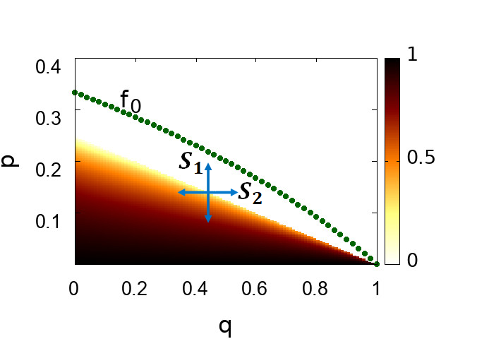
Figure 1: Value of the order parameter in the $p-q$ phase space indicates the existence of the phase boundary given by $p=\frac{1-q}{4}$. The dashed line in the disordered phase represents $f_{0}=\frac{1-q}{3-q}$.

On the other hand, when the steady state (at $t\rightarrow\infty$) is disordered, $f_{+1}=f_{-1}$, which when put in equation 2, one gets

$$f_{+1}=f_{-1}=\dfrac{1}{3-q};f_{0}=\dfrac{1-q}{3-q}..$$ (10)

Interestingly, the above values are independent of $p$.

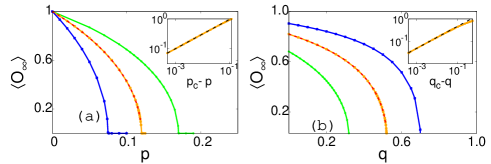
Figure 2: $\langle O_{\infty}\rangle$ calculated numerically by solving eq. 2 and 3 for different sets of values of $q_{c}$ and $p_{c}$ along paths $S_{1}$ and $S_{2}$ respectively on the phase boundary (see Fig. 1). In (a) the curves are for the path $S_{1}$ with fixed critical values of $q$; $q_{c}=0.70,0.52,0.32$ from left to right; in (b) the curves are for the path $S_{2}$ with fixed critical values of $p$; $p_{c}=0.17,0.12,0.075$ from left to right. Analytical values of $\langle O\rangle$ from equation 9 are also plotted with dashed lines for $q_{c}=0.52$ in (a) and $p_{c}=0.12$ in (b). Insets of (a) and (b) show the scaling behaviour of $\langle O\rangle$, indicating $\beta=0.5$

Phase boundary:

At the critical point between ordered-disordered phase transition the fraction $f_{0}$ at the steady state for both the phases should be equal which gives

$$f_{0}=\dfrac{1-q}{3-q}=\frac{qp+p}{qp-p+1}.$$

Hence one gets an equation of a straight line

$$p=\frac{1-q}{4}$$ (11)

which is the phase boundary in the $p-q$ phase space shown in Fig 1. The value of $f_{0}$, a function of $q$ only in the disordered phase, is also shown. Note that the order-disorder boundary obtained at $p=0$ for $q=1$ can be obtained as an analytical continuation from the above equation. However, all results discussed henceforth are for $q\neq 1$ in general.

Behaviour of $\langle O\rangle$ close to a critical point:

Each point on the phase boundary is a critical point. We analyse the behaviour of the order parameter close to a critical point along two different routes $S_{1}$ and $S_{2}$ as indicated in Fig 1. For path $S_{1}$, we take $x=p_{c}-p$ and $q=q_{c}$ to get from equation 9,

$$\langle O\rangle = \frac{2(4x-4q_{c}x-q_{c}^{2}+1\pm 4\sqrt{(1-q_{c})x})}{(4x-q_{c}-8q_{c}x+4q_{c}^{2}x-3q_{c}^{2}+q_{c}^{3}+3)}$$ (12)

$$- \frac{\frac{q_{c}}{2}+2x+\frac{1}{2}}{\frac{q_{c}}{4}+x-q_{c}(\frac{q_{c}}{4}+x-\frac{1}{4})+\frac{3}{4}}.$$

As $x\rightarrow 0$ behaviour of $\langle O\rangle\rightarrow\sqrt{x}$, i.e., the critical exponent $\beta$ is $0.5$ along the path $S_{1}$.

Similarly, for path $S_{2}$, rewriting equation 9 taking $y=q_{c}-q$ and $p=p_{c}$ we get

$$\langle O\rangle = \frac{2p_{c}y-y-4p_{c}+8p_{c}^{2}\pm\sqrt{y(4p_{c}+y)}}{16p_{c}^{3}+8p_{c}^{2}y+p_{c}y^{2}-4p_{c}-y}$$ (13)

$$- \frac{2p_{c}-1}{p_{c}+p_{c}(4p_{c}+y-1)-1}.$$

Thus $\langle O\rangle\rightarrow\sqrt{y}$ as $y\rightarrow 0$ showing that the value of the exponent $\beta=1/2$ does not depend on the path. In fact, the full variation of $\langle O\rangle$ can easily be seen to depend on $[x+4y]^{1/2}$ as the leading order term if we allow both $p$ and $q$ to vary about the critical point as before, i.e., $p=p_{c}-x$ and $q=q_{c}-y$ with the restriction that $x+4y\geq 0$ for a general direction. Note that for $S_{1}$ and $S_{2}$, both $x,y\geq 0$.

We have also numerically solved the time evolution equations to obtain the values of $\langle O(t\rightarrow\infty)\rangle$ along paths $S_{1}$ and $S_{2}$ for a particular point on the phase boundary to find that indeed the results are compatible with $\beta=0.5$ shown in Fig 2.

III.3 Stability Analysis

In the disordered phase, we obtained a fixed point characterised by $f_{+1}=f_{-1}=\frac{1}{3-q}$. As there are three variables, in principle it is possible that in the disordered state, the values of $f_{+1}$ and $f_{-1}$ still evolve remaining the same. However, for the above values there can be no further change and hence we call this the frozen fixed point kb2 .

Stability of this frozen fixed point can be studied by introducing a deviation $\delta$ about it. Taking $f_{+1}=x^{*}+\delta$ and $f_{-1}=x^{*}-\delta$, where $x^{*}=\dfrac{1}{3-q}$, a stability analysis leads to $\delta(t)=\delta_{0}\exp[\gamma t]$. Here $\delta_{0}$ is the initial deviation considered about the fixed point at $t=0$ and

$$\gamma=\frac{1-q-4p}{3-q}.$$ (14)

As $\langle O\rangle=f_{+1}-f_{-1}=2\delta$, we get

$$\langle O\rangle=2\delta_{0}\exp[\gamma t].$$ (15)

The above equation shows that for an initially ordered state, there will be a growth/decay of the order parameter according to the sign of $\gamma$ which changes at $1-q-4p=0$. This is consistent with the phase boundary at $1-q=4p$ and as expected one gets a disordered state even when starting from an ordered state in the disordered phase.

Equation 15 shows that there is a time scale $\tau=\gamma^{-1}$ associated with the dynamics of the growth/decay and $\tau$ diverges at the phase boundary indicating critical slowing down. Once again, the time dependent equations are solved numerically by taking initial states close to the frozen fixed point and the results agree with the above as shown in Fig 3. Since $\tau\propto(1-q-4p)^{-1}$, it diverges with an exponent $1$ which is related to the critical dynamical exponent $z$, this is to be discussed further in the next section.

III.4 Relaxation from a perfectly ordered state

While for initial states with small order, the order parameter will either decay or grow depending on whether one is in the disordered or ordered phase, for a fully ordered initial state the order parameter will decrease in time in the in both phases. We study the relaxation behaviour by numerically solving the rate equations taking initial condition $f_{+1}=1$.

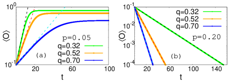
Figure 3: The time evolution of $\langle O\rangle$ generated numerically from eq. 2 and 3 for $\frac{1-q}{4}>p$ (ordered phase) and $\frac{1-q}{4}<p$ (disordered phase) are shown in (a) and (b) respectively with the initial configuration $f_{+1}=x^{*}+\delta_{0}$ and $f_{-1}=x^{*}-\delta_{0}$ (see text). The dotted line in each graph represents the fitted graph following equation 15.

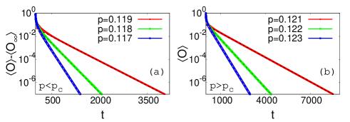
Figure 4: Time evolution of $\langle O\rangle$ calculated by numerically solving eq. 2 and 3 with a fixed value of $q=0.52$ and different values of $p$ (a) below and (b) above the corresponding $p_{c}$ when the initial condition is $(f_{+},f_{0},f_{-1})=(1,0,0)$. The dotted lines show the fitted curve with equation 16.

In the disordered phase the decay of the order parameter is expected to follow Eq 15 at late times as it comes closer to the frozen fixed point, indicating again the presence of a time scale $\propto|\gamma|^{-1}$. In the ordered phase, the order parameter will initially decay and then attain a nonzero saturation value. We find that both behaviour are captured by a single equation

$$(\langle O\rangle-\langle O_{\infty}\rangle)\propto\exp[-t/\tau_{R}]$$ (16)

where $\langle O_{\infty}\rangle$ is the ensemble averaged equilibrium value of the ordered parameter at $t\rightarrow\infty$. We have plotted the data for some particular points above and below the phase boundary in Fig 4, and the timescales $\tau_{R}$ extracted from the slopes of the log-linear graphs are shown in Fig. 5a,b. The results show that $\tau$ and $\tau_{R}$ have identical scaling behaviour in the disordered phase as argued above, while in the ordered phase also, $\tau_{R}$ diverges close to the critical point with the same exponent 1 (see Fig 5c,d)

Lastly, we plot $\langle O\rangle$ as a function of time at several points exactly on the phase boundary in Fig. 6 to get a power law decay with an exponent close to 0.5. This discussion of course excludes the $q=1$ point which is unique, one can easily check that with the critical value $p=0$ here, no evolution of the initially fully ordered state is possible.

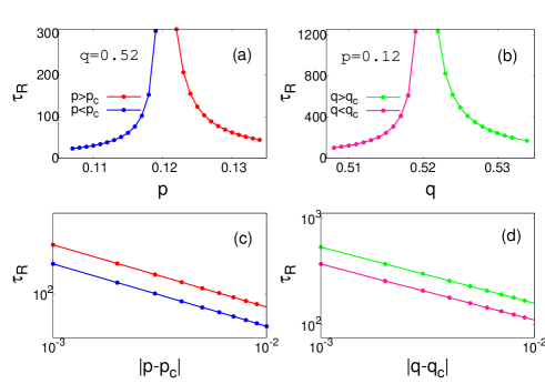
Figure 5: The time scale $\tau_{R}$ calculated from the slopes of the log-linear plots in Fig 4 using equation 16 is shown (a) against $p$ for a constant value of $q$ and (b) against $q$ for a constant value of $p$. In (c) and (d), these values of $\tau_{R}$ are plotted against $|p-p_{c}|$ and $|q-q_{c}|$ respectively, both above and below the critical values to show a power law divergence with the associated exponent very close to unity. The color codes for the upper and lower panels are same.

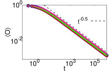
Figure 6: Time variation of $\langle O\rangle$ calculated by numerically solving eq. 2 and 3 exactly at different critical points on the phase boundary indicates $O(t\rightarrow\infty)\propto t^{-0.5}$ .

IV Summary and Discussions

In this paper, we have studied the case of extreme switches in opinion in a three-state kinetic exchange model where the interactions may be both positive as well as negative. The two parameters characterising the probabilities of the extreme switches and negative interactions are $q$ and $p$ respectively. Our main findings are
$\bullet$ The presence of a phase boundary given by $p=\frac{1-q}{4}$
$\bullet$ Exponent $\beta$ associated with the order parameter is universal with the value $1/2$
$\bullet$ The phase boundary can also be obtained using stability analysis. Additionally one gets the time evolution of the partially ordered state showing exponential growth/decay. The associated time scale $\tau$ diverges with an exponent $-1$.
$\bullet$ Relaxation behaviour of the fully ordered state shows the expected exponential decay of the order parameter with time in the disordered phase; for the ordered phase, it relaxes exponentially to a saturation value. The relaxation timescale $\tau_{R}$ and $\tau$ have identical scaling behaviour. Exactly on the phase boundary, the order parameter shows a power law decay.
$\bullet$ The overall behaviour is mean field like for $q\neq 1$.
$\bullet$ The $q=1,p=0$ has a special significance.

While the first four issues have already been discussed in detail in the previous section, we focus on the last two points here. It had been already known that in the mean field three state kinetic exchange model without extreme switches, the value of the exponent $\beta=1/2$. Also, assuming the mean field model has an effective dimension $d$, the exponent $\bar{\nu}=\nu d=2$ was obtained previously where $\nu$ is the correlation length exponent BCS . We have found $\beta$ to be equal to 1/2 at any point on the phase boundary in the two parameter model for $q\neq 1$. To get $\bar{\nu}$, we conduct small scale simulations about a particular point on the phase boundary. Indeed the scaled order parameter curves collapse when plotted against $|\epsilon|N^{1/{\bar{\nu}}}$, where $\epsilon$ denotes the deviation from the critical point, with $\beta=1/2$ and $\bar{\nu}=2$. The raw data and the collapse are shown in Fig 7. Hence the static critical behaviour is unaffected by the parameter $q\neq 1$.

The critical slowing down phenomena is observed with a timescale diverging as $|\epsilon|^{-1}$, again independent of $q$. Since in a continuous phase transition, the time scale diverges as $\xi^{z}$ where $\xi$ is the correlation length $\propto|\epsilon|^{-\nu}$ and $z$ the dynamic critical exponent, one gets $\tau\propto|\epsilon|^{-\nu z}$. Hence our results indicate $\nu z=1$.

Next one can consider the relaxation of the order parameter exactly at criticality. The power law behaviour $t^{-1/2}$ can be shown to be compatible with the theory of dynamic critical phenomena. In general the dynamical behaviour of the order parameter is given by $O(t)\propto t^{-y}f(t/\xi^{z})$ with $O(t)\propto t^{-y}$ exactly at the critical point. Equilibrium behaviour indicates $y=\beta/\nu z$. Therefore, using the values $\beta=1/2$ and $\nu z=1$, one gets $y=1/2$, which is the value obtained here. We also remark that the values of the static and dynamic exponents obtained here coincide with those of the mean field Ising model ($\beta=1/2,\nu=1/2,z=2$) if one uses $d=4$, the upper critical dimension of the Ising model.

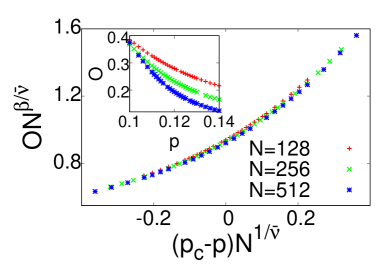
Figure 7: Simulation results: Data collapse of the scaled order parameter $ON^{\beta/\bar{\nu}}$, when plotted against $(p_{c}-p)N^{1/\bar{\nu}}$ for a fixed value of $q=0.52$, is obtained using the values $\bar{\nu}=2.0$ and $\beta=0.5$. Inset shows the raw data.

Even though the critical behaviour is unchanged with a nonzero value of $q$, we note that the fixed point values are independent of $p$ in the disordered phase. Also, the variation of $f_{0}$ in the disordered phase (see Fig. 1) suggests that as $q$ is increased, the model tends to become a binary one. The interpretation is, with increasing probability of extreme switches, the system in the disordered phase tends to be polarised as it becomes increasingly difficult to retain a neutral opinion.

For $q=1$, we get two equations (5 and 6) after a transient time when $f_{0}$ becomes zero. These can be easily identified as the equations governing the dynamics of a two state voter model with random flipping probability $p$. Obviously, it becomes disordered at any value of $p$. Previously it was noted that for $p=0$, the model is identical to the mean field voter model for $q=1$, with $p\neq 0$ we thus obtain a mapping to a voter model with random flipping.

Hence the main conclusion from the present study is that the extreme switches act as additional noise for the model considered in BCS thereby lowering the critical values $p_{c}$ without changing the critical behaviour. The point $q=1$ has a special interpretation. The role of the two kinds of disorder are however different, the system becomes disordered for a finite value of $p$ (for $q=0$) but remains ordered up to the extreme value of $q$ (for $p=0$) kb2 . It is, therefore, not surprising that the critical behaviour is dominated by $p$ while $q$ acts as an irrelevant variable. However, the nature of the disordered phase is dictated by $q$ alone.

The results obtained in the present paper are based on the mean field dynamical equations. Of course, if we consider the system on lattices with nearest neighbour coupling, there will be quantitative changes. As a future study, it will be interesting to investigate how the extreme switches affect qualitatively the criticality and dynamics in finite dimensions.

Acknowledgement

PS acknowledges financial support from SERB (Government of India) through scheme no MTR/2020/000356. We thank Sudip Mukherjee, Soumyajyoti Biswas and Arnab Chatterjee for some discussions.

References

- (1) C. Castellano, S. Fortunato, V. Loreto, Statistical physics of social dynamics, Rev. Mod. Phys. 81, 591 (2009).
- (2) P. Sen, B. K. Chakrabarti, Sociophysics: An Introduction, Oxford University Press, Oxford (2014).
- (3) S. Galam, Sociophysics: A Physicist’s Modeling of Psycho-political Phenomena, Springer, Boston, MA (2012).
- (4) F. Vazquez, P. L. Krapivsky, S. Redner, Constrained opinion dynamics: freezing and slow evolution J. Phys. A: Math. Gen. 36 L61 (2003).
- (5) F. Vazquez and S. Redner, Ultimate Fate of Constrained Voters, J. Phys. A 37, 8479 (2004).
- (6) X. Castelló, V. M. Eguíluz and M. San Miguel, Ordering dynamics with two non-excluding options: bilingualism in language competition, New Journal of Physics 8, 308 (2006).
- (7) L. Dall’Asta and T. Galla, Algebraic coarsening in voter models with intermediate states, Journal of Physics A: Mathematical and Theoretical, 41, 435003 (2008).
- (8) X. Castelló, A. Baronchelli, V. Loreto, Consensus and ordering in language dynamics, Eur. Phys. J. B 71, 557 (2009).
- (9) M. Mobilia, Fixation and Polarization in a Three-Species Opinion Dynamics Model, Europhys Lett 95 50002 (2011).
- (10) S. Biswas, A. Chaterjee, P. Sen, Disorder induced phase transition in kinetic models of opinion formation, Physica A 391, 3257 (2012).
- (11) S. Biswas, Mean-field solutions of kinetic-exchange opinion models, Phys. Rev. E 84, 056106 (2011).
- (12) N. Crokidakis, C. Anteneodo, Role of conviction in nonequilibrium models of opinion formation, Phys. Rev. E 86, 061127 (2012).
- (13) N. Crokidakis, Phase transition in kinetic exchange opinion models with independence, Phys. Lett. A 378, 1683 (2014).
- (14) S. Mukherjee, A. Chatterjee, Disorder-induced phase transition in an opinion dynamics model: Results in two and three dimensions, Phys. Rev. E 94, 062317 (2016).
- (15) F. W. S. Lima, J. A. Plascak, Kinetic models of discrete opinion dynamics on directed Barabasi-Albert networks, Entropy 2019, 942 (2019).
- (16) S. Mukherjee, S. Biswas and P. Sen, Long route to consensus: Two stage coarsening in a binary choice voting model, Phys. Rev. E 102, 012316 (2020).
- (17) K. Biswas and P. Sen,Non-equilibrium dynamics in a three-state opinion-formation model with stochastic extreme switches, Phys. Rev. E 106, 054311 (2022).
- (18) T. Hadzibeganovic, D. Stauffer, C. Schulze C, Boundary effects in a three-state modified voter model for languages Physica A, 387, 3242 (2008).
- (19) S. Gekle, L. Peliti and S. Galam, Opinion dynamics in a three-choice system. Eur. Phys. J. B 45, 569 (2005).
- (20) S. Galam, The Drastic Outcomes from Voting Alliances in Three-Party Democratic Voting (1990 2013), J. Stat. Phys. 151, 46 (2013).
- (21) S. Biswas, P. Sen, Critical noise can make the minority candidate win: The U.S. presidential election cases, Phys. Rev. E 96, 032303 (2017).
- (22) K. Biswas, S. Biswas and P. Sen, Block size dependence of coarse graining in discrete opinion dynamics model: Application to the US presidential elections, ‘ Physica A: Statistical Mechanics and its Applications 566, 125639 (2021).