Design of Hamiltonian Monte Carlo for perfect simulation of general continuous distributions

Abstract

Hamiltonian Monte Carlo (HMC) is an efficient method of simulating smooth distributions and has motivated the widely used No-U-turn Sampler (NUTS) and software Stan. We build on NUTS and the technique of “unbiased sampling” to design HMC algorithms that produce perfect simulation of general continuous distributions that are amenable to HMC. Our methods enable separation of Markov chain Monte Carlo convergence error from experimental error, and thereby provide much more powerful MCMC convergence diagnostics than current state-of-the-art summary statistics which confound these two errors. Objective comparison of different MCMC algorithms is provided by the number of derivative evaluations per perfect sample point. We demonstrate the methodology with applications to normal, $t$ and normal mixture distributions up to 100 dimensions, and a 12-dimensional Bayesian Lasso regression. HMC runs effectively with a goal of 20 to 30 points per trajectory. Numbers of derivative evaluations per perfect sample point range from 390 for a univariate normal distribution to 12,000 for a 100-dimensional mixture of two normal distributions with modes separated by six standard deviations, and 22,000 for a 100-dimensional $t$-distribution with four degrees of freedom.

Keywords: Coupling from the past; Hybrid Monte Carlo; Markov chain Monte Carlo; MCMC convergence diagnostics; No U-Turn Sampler; Unbiased simulation

1 Introduction

The Monte Carlo method has become an indispensable tool in science, engineering and finance (Kroese et al., 2014). In its ideal form it provides a perfect sample of independent random objects from a specified distribution. Often the practitioner accepts much less than this ideal, especially when the only feasible means of sample generation is Markov chain Monte Carlo (MCMC). Tests for convergence of MCMC to the target distribution are most commonly based on the Gelman–Rubin statistic (Gelman and Rubin, 1992), rely on large-sample asymptotic decay of test statistics and confound convergence error with experimental error (see review in Roy, 2020). Moreover, objects generated by MCMC generally exhibit autocorrelation (Gelman and Shirley, 2011, sec. 6.7).

Perfect simulation overcomes the above drawbacks by generating objects that exactly follow the target distribution and are independent (see reviews by Craiu and Meng, 2011; Huber, 2016). Few problems are currently amenable to perfect simulation.

Hamiltonian Monte Carlo (HMC) (Duane et al., 1987; Neal, 1993, 1995, 2011) efficiently simulates smooth distributions and has motivated the No-U-Turn Sampler (NUTS) (Hoffman and Gelman, 2014) and software Stan (Carpenter et al., 2017).

This paper presents advances in design of algorithms for HMC (section 2) and perfect simulation (Section 3). We build on NUTS to design two new HMC algorithms: the NUTS4 algorithm which operates on groups of four trajectory points and, through earlier detection of U-turns, reduces the number of discarded points; and the Full Random Uniform Trajectory Sampler (FRUTS, pronounced “fruits”), which discards at most one point at each end of a trajectory. We present a new method of setting the time step, a critical HMC parameter, and describe the numbering of HMC trajectory points which is integral to perfect simulation. Sections 4 and 5 demonstrate the methods on a range of standard distributions and a challenging real-world problem.

Compared to current MCMC practice, our methods offer the advantages of decoupling convergence error from experimental error, replacing asymptotic convergence tests by perfect simulation in an exact number of iterations, and producing independent samples. Our methods are widely applicable to continuous distributions with differentiable likelihoods.

2 Design of Hamiltonian Monte Carlo algorithms

2.1 Review of Hamiltonian Monte Carlo

HMC, originally known as “Hybrid Monte Carlo” (Duane et al., 1987) from its alternation of random and deterministic steps, simulates a $d$-dimensional vector $q$ by introducing a time variable $t$ and a $d$-dimensional “momentum” vector $p$. It defines the Hamiltonian as $H=U+K$, where potential energy $U$ is the negative log-likelihood of $q$, and kinetic energy $K$ is a positive, differentiable function of $p$ satisfying $K(-p)=K(p)$. We assume the form

$$K=|p|^{\beta}/\beta$$ (1)

where $|p|$ is the Euclidean norm and $\beta>0$. The only commonly used setting is $\beta=2$.

HMC (Algorithm 1) samples $p$ independently from the likelihood proportional to $\exp(-K)$ and calculates a deterministic trajectory, analogous to the orbit of a particle with position $q$ and momentum $p$, according to Hamilton’s equations of motion (Hamilton, 1834, 1835):

$$\dot{q}=\partial H/\partial p=dK/dp,\quad\dot{p}=-\partial H/\partial q=-dU/dq,$$ (2)

where dots denote differentiation with respect to time. Under assumption (1),

$$\dot{q}=\left(dK/{d|p|}\right)p/|p|=|p|^{\beta-2}p.$$ (3)

Algorithm 1 Hamiltonian Monte Carlo for a general Trajectory function, defined later

1:global $U,K,DU,DK,\delta t,d,d_{R}$ $\triangleright$ Energy and derivatives, time step, dimensions

2:procedure HMC($q_{\text{st}},n_{T},R$) $\triangleright$ $R$: Random number matrix $n_{T}\times d_{R}$, indexed $[i_{T},j]$

3:     $q_{0}\leftarrow q_{\text{st}}$ $\triangleright$ Set starting point.

4:     for $i_{T}\leftarrow 1:n_{T}$ do $\triangleright$ $i_{T}$, $n_{T}$: trajectory count, number of trajectories

5:         $\triangleright$ Sample momentum independently at the start of each trajectory.

6:         sample $p_{0}\sim e^{-K}$ using $R[i_{T},j_{\text{mom}}]$ $\triangleright$ $j_{\text{mom}}$: momentum random number index

7:         $H_{0}\leftarrow U(q_{0})+K(p_{0})$ $\triangleright$ Calculate Hamiltonian at origin.

8:         $\triangleright$ Run the trajectory and select a destination point: may run for a fixed time

9:         $\triangleright$ period (original HMC), or select randomly from trajectory points (NUTS).

10:         $(q,p)\leftarrow$ Trajectory($q_{0},p_{0},R[i_{T},j_{\text{traj}}]$) $\triangleright$ $j_{\text{traj}}$: Trajectory random numbers

11:         $H\leftarrow U(q)+K(p)$ $\triangleright$ Calculate Hamiltonian at destination.

12:         if $R[i_{T},j_{\text{MH}}]\leq\exp(H_{0}-H)$ then $q_{0}\leftarrow q$ $\triangleright$ $j_{\text{MH}}$: M–H test random number

13:         $\triangleright$ Destination $q_{0}$ is origin of next trajectory. If M–H test fails, $q_{0}$ is unchanged.

14:     end for

15:     return $q_{0}$

16:end procedure

Hamilton’s equations (2) endow trajectories with properties that ensure reversibility or “detailed balance” and establish that the stationary distribution of HMC is the target distribution (see, e.g., Neal, 2011): 1. Volume is preserved: a region in ($q$, $p$) space is mapped to a region with the same volume. 2. Trajectories are reversible: negating the momentum at any point and applying the dynamics (2) retraces the trajectory back to its origin. 3. The value of the Hamiltonian $H$ is preserved.

In practice, the dynamics (2) have to be discretized in time and the leapfrog algorithm retains properties 1 and 2 (see, e.g., Duane et al., 1987). Given an origin $q_{0}$ and initial momentum vector $p_{0}$ at time zero, leapfrog calculates $q$ at integer multiples of the time step $\delta t$, and $p$ at integer-plus-a-half multiples. It does not exactly preserve the value of $H$ but compensates by inserting a Metropolis–Hastings update, whereby if the value of $H$ increases by an amount $\delta H$ from the origin to the destination, the new value of $q$ is accepted with probability $e^{-\delta H}$. In case of rejection the destination is reset to the origin (Metropolis et al., 1953; Hastings, 1970; Duane et al., 1987).

2.2 New HMC algorithms

The original HMC trajectories of Duane et al. (1987), which we call “raw” HMC, simply travelled for a fixed number of points along the trajectory. For comparison with other algorithms, we set raw HMC to travel ten points forward and ten points backward from the origin, making a total of 21 points, close to our target number of points in the advanced algorithms (NUTS, NUTS4 and FRUTS). We chose the destination point randomly and uniformly from these 21 points, in the same way as the advanced algorithms do.

The No U-Turn Sampler (Hoffman and Gelman, 2014) was a major advance in HMC algorithm design. Because NUTS discards up to half its eligible trajectory points, we designed two new algorithms, which we call NUTS4 and the Full Random Uniform Trajectory Sampler (FRUTS). NUTS4 is a modification to NUTS to detect U-turns earlier and reduce the number of discarded points, while FRUTS is designed differently to discard at most one point at each end of a trajectory. We present NUTS4 in detail in Algorithm 2, as it performed the best in the majority of our tests. The advantage of FRUTS in greatly reducing the number of discarded points was frequently outweighed by the orientation of NUTS and NUTS4 trajectories roughly parallel to the initial momentum, instead of random as in FRUTS. FRUTS is described in detail in section S1 of Supplementary Material.

In NUTS4 we make three innovations to NUTS. Firstly, we follow the philosophy of the leapfrog algorithm in calculating the momentum vector $p$, as far as possible, at only integer-plus-a-half time points, as opposed to the integer time points used in NUTS. This change delays termination of a trajectory until the discrete trajectory turns back on itself, instead of forcing termination as soon as a U-turn is detected in continuous time. It also saves an evaluation of the derivative $dU/dq$ at each end of the trajectory, except when the trajectory’s randomly chosen destination point happens to be an endpoint.

The second innovation in NUTS4 is more frequent testing for U-turns, to detect a U-turn earlier and reduce the number of discarded points. A trajectory is divided into disjoint segments of four consecutive points which are the minimum units on which U-turn tests are conducted. Our tests use the internal momentum vectors half-way between points 1 and 2, and between points 3 and 4 of a segment. The arc from every segment to every other segment is also tested for a U-turn. This more intensive testing is facilitated by control of the number of points in a trajectory through our setting of the time step (see section 2.3), which keeps the total number of tests manageable.

Our third innovation is to impose a minimum of 16 and a maximum of 256 on the number of points in a trajectory. Again, this is facilitated by our setting of the time step, which operates to a goal of about 20 points per trajectory. The three innovations do not affect the proof of detailed balance for NUTS given by Hoffman and Gelman (2014), because all four-point segments, and pairs of segments, are treated equally.

Algorithm 2 NUTS4 trajectory for use in Algorithm 1: Setup and forward flop

1:procedure Trajectory($q_{0},p_{0},r$) $\triangleright$ $r$: Vector of random numbers, indexed by $[j]$

2:     $i^{+}\leftarrow i^{-}\leftarrow 0$; $q_{\text{traj}}[0,]\leftarrow q^{+}\leftarrow q^{-}\leftarrow q_{0}$ $\triangleright$ $q_{\text{traj}}[i^{-}:i^{+},]$ stores trajectory points.

3:     $p_{\text{traj}}[0,]\leftarrow p_{0}$; $\dot{p}_{0}\leftarrow-DU(q_{0})$; $\text{Uturn}\leftarrow\textbf{false}$ $\triangleright$ $p_{\text{traj}}[i^{-}:i^{+},]$ stores momentum.

4:     $p^{+}\leftarrow p_{0}^{+}\leftarrow p_{0}+{\scriptstyle\frac{1}{2}}\delta t\,\dot{p}_{0}$; $p^{-}\leftarrow p_{0}^{-}\leftarrow p_{0}-{\scriptstyle\frac{1}{2}}\delta t\,\dot{p}_{0}$ $\triangleright$ $p_{0}^{+},p_{0}^{-}$: Half time-step offset of $p_{0}$

5:     for $i_{\text{flop}}\leftarrow 1:n_{\text{flop}}$ do $\triangleright$ “Flop” by $2^{i_{\text{flop}}-1}$ points to one side, up to max length.

6:         if $r[j_{\text{flop}}+i_{\text{flop}}]\geq 0.5$ then $\triangleright$ $j_{\text{flop}}$: Offset for flops; ${\scriptstyle\frac{1}{2}}$–${\scriptstyle\frac{1}{2}}$ forward or backward

7:              $i^{+}_{\text{new}}\leftarrow i^{+}+2^{i_{\text{flop}}-1}$ $\triangleright$ New value of $i^{+}$, if flop doesn’t produce a U-turn

8:              for $i\leftarrow(i^{+}+1):i^{+}_{\text{new}}$ do $\triangleright$ Hamiltonian dynamics: $p$ already done if $i=1$

9:                  if $i>1$ {$\dot{p}\leftarrow-DU(q^{+})$; $p^{+}\leftarrow p^{+}+\delta t\,\dot{p}$} $\triangleright$ $p^{+}$ is at time $(i-{\scriptstyle\frac{1}{2}})\delta t$.

10:                  $\dot{q}\leftarrow DK(p^{+})$; $q^{+}\leftarrow q^{+}+\delta t\,\dot{q}$ $\triangleright$ Unconditional; $q^{+}$ is at time $i\,\delta t$.

11:                  if $i-i^{+}=0$ mod 4 then $\triangleright$ Test for U-turn every fourth point.

12:                       for $i_{\text{test}}\leftarrow i^{-}:(i-3):4$ do $\triangleright$ Current and previous segments

13:                           $q_{\text{span}}\leftarrow q^{+}-q_{\text{traj}}[i_{\text{test}},]$; $\text{Uturn}\leftarrow q_{\text{span}}\cdot p_{\text{traj}}[i_{\text{test}}+(i_{\text{test}}\geq 0),]<0$

14:                           $\quad\textbf{or }q_{\text{span}}\cdot p^{+}<0$; if Uturn break $\triangleright$ Skip over $p_{\text{traj}}[0,]$.

15:                       end for

16:                  end if$\triangleright$ Next statement enforces minimum trajectory length 16 points.

17:                  if Uturn and $i_{\text{flop}}>4$ break else {$q_{\text{traj}}[i,]\leftarrow q^{+}$; $p_{\text{traj}}[i,]\leftarrow p^{+}$}

18:              end for$\triangleright$ Next: Confirm valid flop and handle flop to backward side.

19:              if Uturn and $i_{\text{flop}}>4$ break else $i^{+}\leftarrow i^{+}_{\text{new}}$ $\triangleright$ Alg. continues below.

Algorithm 3 NUTS4 trajectory: Backward flop and selection of destination point

20:         else$\triangleright$ Random flop direction is to backward side.

21:              $i^{-}_{\text{new}}\leftarrow i^{-}-2^{i_{\text{flop}}-1}$ $\triangleright$ New value of $i^{-}$, if flop doesn’t produce a U-turn

22:              for $i\leftarrow(i^{-}-1):i^{-}_{\text{new}}:-1$ do $\triangleright$ Hamiltonian dynamics: $p$ done if $i=-1$

23:                  if $i<-1$ {$\dot{p}\leftarrow-DU(q^{-})$; $p^{-}\leftarrow p^{-}-\delta t\,\dot{p}$} $\triangleright$ $p^{-}$ is at time $(i+{\scriptstyle\frac{1}{2}})\delta t$.

24:                  $\dot{q}\leftarrow DK(p^{-})$; $q^{-}\leftarrow q^{-}-\delta t\,\dot{q}$; $\triangleright$ Unconditional; $q^{-}$ is at time $i\,\delta t$.

25:                  if $i^{-}-i=0$ mod 4 then $\triangleright$ Test for U-turn every fourth point.

26:                       for $i_{\text{test}}\leftarrow i^{+}:(i+3):-4$ do $\triangleright$ Current and previous segments

27:                           $q_{\text{span}}\leftarrow q_{\text{traj}}[i_{\text{test}},]-q^{-}$; $\text{Uturn}\leftarrow q_{\text{span}}\cdot p_{\text{traj}}[i_{\text{test}}-(i_{\text{test}}\leq 0),]<0$

28:                           $\quad\textbf{or }q_{\text{span}}\cdot p^{-}<0$; if Uturn break $\triangleright$ Skip over $p_{\text{traj}}[0,]$.

29:                       end for

30:                  end if$\triangleright$ Next statement enforces minimum trajectory length 16 points.

31:                  if Uturn and $i_{\text{flop}}>4$ break else {$q_{\text{traj}}[i,]\leftarrow q^{-}$; $p_{\text{traj}}[i,]\leftarrow p^{-}$}

32:              end for

33:              if Uturn and $i_{\text{flop}}>4$ break else $i^{-}\leftarrow i^{-}_{\text{new}}$ $\triangleright$ Confirm valid flop.

34:         end if;  if Uturn and $i_{\text{flop}}=4$ break $\triangleright$ Break if U-turn at 16 points.

35:     end for$\triangleright$ End of $i_{\text{flop}}$ loop

36:     $\triangleright$ Select the destination randomly and uniformly using variate $r[j_{\text{sel}},]\sim U(0,1).$

37:     $i_{\text{dest}}\leftarrow i^{-}+\textbf{floor}(\{i^{+}-i^{-}+1\}\times r[j_{\text{sel}}])$ $\triangleright$ $i^{+}-i^{-}+1=$ no. of trajectory points.

38:     return $(q_{\text{traj}}[i_{\text{dest}},],p_{\text{traj}}[i_{\text{dest}},])$ $\triangleright$ Code omitted: Advance $p$ by $\pm{\scriptstyle\frac{1}{2}}\delta t$ if $i_{\text{dest}}\neq 0$.

39:end procedure

2.3 Setting the time step

We set the time step $\delta t$ to produce a practical number of trajectory points for effective sampling and an acceptable probability of passing the Metropolis–Hastings test (line 12 of Algorithm 1). The setting is derived in Supplementary section S2:

$$\delta t=2h\beta^{1/\beta-1}\alpha^{1/\alpha}\,\frac{\Gamma(d/\beta)}{\Gamma\big{(}\{d-1\}/\beta+1\big{)}}\cdot\frac{\Gamma\big{(}\{d-1\}/\beta+d/\alpha+1\big{)}}{\Gamma\big{(}\{d-1\}/\beta+\{d-1\}/\alpha+1\big{)}}\,,$$ (4)

where $1/h$ is the desired number of sample points and $\alpha$ depends on the target distribution which is assumed to have approximately unit variance. Typically $h=0.05$ for 20 points per trajectory, $\alpha=2$ for a short-tailed target distribution and $\alpha<2$ for a long-tailed one.

2.4 Selection of the destination point

We number the points in a trajectory in the forward direction of the trajectory, as shown in Figure 1. As in NUTS, we select the destination randomly from the trajectory points. We use a uniform random number to specify the destination point number (Algorithm 2, line 37). Coalescence of coupled processes, which is enabled by this method of destination selection and also shown in Figure 1, will be described in section 3.2.

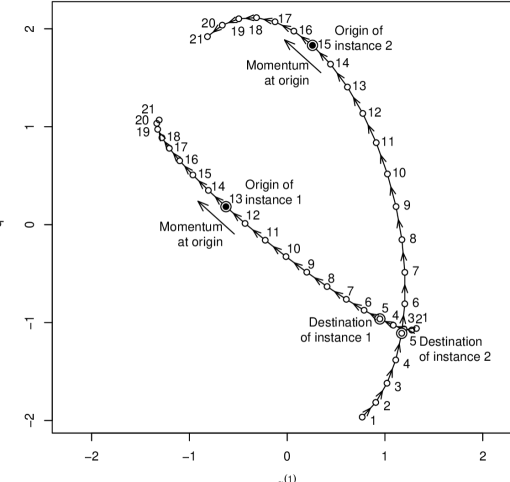
Figure 1: Numbering of trajectory points in forward direction for coupled instances of a trajectory with different origins but the same random numbers. Selection of the destination points is also coupled and gradually brings the instances closer together.

3 Perfect simulation

3.1 Review of perfect simulation

Perfect simulation algorithms are diverse and include multigamma coupling (Murdoch and Green, 1998), strong stationary stopping times (Aldous and Diaconis, 1987) and perfect slice sampling (Mira et al., 2001). These algorithms are generally difficult to use and not widely applicable. Multigamma coupling has an impossibly small probability of satisfying the conditions for perfect simulation for most practical problems. Perfect slice sampling has the difficulty of establishing, at least approximately, the boundary of the feasible space, which leads to a curse of dimensionality (Bellman, 1955) in high numbers of dimensions.

The most versatile existing perfect simulation algorithm is coupling from the past (CFTP) (Propp and Wilson, 1996), but even that algorithm’s applicability has to date been limited to a small subset of the total range of problems suitable for MCMC. CFTP produces coalescence of random objects to the same outcome from different starting points, and constitutes perfect simulation when it can be proven that the same outcome occurs from every possible starting point. CFTP samples forward in time and prepends extra random numbers as needed to the beginning of the sequence, not the end, thereby avoiding bias towards “easier” sets of random numbers that produce faster coalescence. The variant “read-once coupling from the past” (ROCFTP) (Wilson, 2000) proceeds only in forward sequence, in blocks of fixed length, some of which exhibit coalescence while others may not.

Some processes possess a monotonicity property that allows proof of coalescence from every possible starting point, to establish perfect simulation by CFTP (Propp and Wilson, 1996). In general, monotonicity is not available and even a discrete-valued process whose transition probabilities are a priori not known numerically but are calculated on the run would have to visit every possible state to establish perfect simulation with CFTP or ROCFTP (Lovász and Winkler, 1995; Fill, 1998, p. 135). Continuous processes with non-countable states magnify this difficulty.

Although not presented as a perfect simulation technique, “unbiased simulation” (Glynn and Rhee, 2014; Jacob et al., 2020) estimates expectations of functions of coalescent random processes. It does not require monotonicity or a multitude of starting points, and its absence of bias is exact. Its disadvantage is that its output consists not of coalesced samples but of lengthy sums that can vary wildly and even produce values outside the allowed space, such as histogram probability values that are negative or greater than 1.

Unbiased simulation takes coupled random processes $X$ and $Y$ with the same starting point or distribution of starting points (Jacob et al., 2020, p. 545). The processes’ random numbers are offset by one iteration: the transition from the starting point $Y_{0}$ of $Y$ to the next value $Y_{1}$ uses the same random numbers as that from $X_{1}$ to $X_{2}$. An unbiased sample for the expectation of the ergodic distribution of some function which we denote $g(X)$ is

$$g(X_{k})+\sum_{i=k+1}^{\infty}\{g(X_{i})-g(Y_{i-1})\},$$ (5)

where $k\geq 0$ is some chosen burn-in-like number of iterations. Processes $X$ and $Y$ are designed to coalesce, so that for some random number of iterations $\tau$, $g(X_{i})=g(Y_{i-1})$ for all $i\geq\tau$ and the above infinite sum actually contains only a finite number of terms.

We show in section 3.3 below that unbiased simulation becomes perfect simulation when $k$ is made large enough that the probability of a non-empty sum in (5) becomes vanishingly small. We propose a new algorithm to take advantage of the resulting large values of $k$.

3.2 Coalescence in HMC

Gradual coalescence over successive HMC trajectories, enabled by consistent numbering of trajectory points and use of the same random numbers with different starting points, has been illustrated in Figure 1. We convert gradual coalescence into exact coalescence by a final rounding step to a congruence (Algorithm 4). For detailed balance, the desired congruence in each coordinate is sampled randomly and uniformly modulo some small interval width $w$, similarly to a random, uniform Metropolis–Hastings jump. Any change in negative log-likelihood $U$ is accounted for by a Metropolis–Hastings test.

Algorithm 4 Coalescence in HMC, calling HMC (Algorithm 1) and rounding

1:procedure HmcRound($q_{\text{st}},n_{T},R,r_{\text{ro}},w$) $\triangleright$ $r_{\text{ro}}$, $w$: rounding random vector & width

2:     $q\leftarrow\textsc{HMC}(q_{\text{st}},n_{T},R)$ $\triangleright$ $q_{\text{st}}$, $R$: initial value, matrix of random numbers

3:     $q_{\text{ro}}\leftarrow w\times\{\textbf{floor}(q/w)+r_{\text{ro}}[1:d]\}$ $\triangleright$ Make outcomes identical if already close.

4:     if $r_{\text{ro}}[d+1]\leq\exp\{U(q)-U(q_{\text{ro}})\}$ then $q\leftarrow q_{\text{ro}}$ $\triangleright$ M–H test for rounding

5:     $\triangleright$ Note $r_{\text{ro}}$ has length $d+1$. Failure of M–H test means no exact coalescence.

6:     return $q$

7:end procedure

Challenging starting points should be chosen to explore coalescence in problems in which no monotonicity property is available (see section 3.1). For HMC, challenging points comprise both extreme points and points of high likelihood where potential energy $U$ is low and may provide insufficient energy to reach a destination point that is reachable from an extreme starting point. Our CFTP examples use $m=\min(2^{d}+1,33)$ starting points, comprising $m-1$ extreme points and the maximum-likelihood point; the mixture examples add an extra equal-maximum-likelihood point. Coordinate values of extreme points are $\pm 6$ in scaled coordinates that have approximately unit variance (see section 2.3 and Supplementary section S2). For $d\leq 5$ the extreme points follow a $2^{d}$ factorial design, while for $d>5$ the first five co-ordinates are factorial and the others are set randomly to $\pm 6$.

3.3 From unbiased simulation to perfect simulation

The sample point (5) is valid for any function $g$, including a histogram with arbitrarily narrow intervals. Therefore the “string” of pairs of values and sample weights $\{(X_{k},1)$, $(Y_{k},-1)$, $\ldots$, $(X_{\tau-2},1)$, $(Y_{\tau-2},-1)$, $(X_{\tau-1},1)\}$ is an unbiased estimator of the distribution of $X$; i.e., it constitutes a perfect sample point from the distribution, with the proviso that it may contain multiple points and negative weights. A sample weight of $-1$ indicates a “hole” that, in a large sample of many strings, will be cancelled out by an equal value (or a value in the same histogram bar) that has a weight of $+1$ in some other string.

Negative weights do not occur if the sum in (5) is empty; i.e., if the processes $X$ and $Y$ coalesce within $k$ steps. Therefore a perfect sample is obtained if $k$ is chosen large enough that the probability of lack of coalescence within $k$ steps is vanishingly small; e.g, smaller than the numerical precision used in the arithmetic.

We emphasize that a target distribution should be thoroughly investigated both theoretically and numerically before the value of $k$ is set. The consequences of negative weights are severe, as a single string can be very long and contain many negative weights, e.g., when one region of the sample space is almost cut off from the rest in a multi-modal distribution, and this is not appreciated before setting $k$. Negative weights express the reality that, when theory such as monotonicity from a finite set of starting points is not available, perfect simulation requires exploration of the entire sample space (see section 3.1). The potential for negative weights provides reassurance that unbiased sampling operates within established laws and can produce perfect simulation without visiting every possible state of a process.

Algorithm 4 substitutes an “iteration” in (5) by a “block” of $n_{T}$ HMC trajectories, followed by a single rounding step. Our examples set $n_{T}$ so that approximately 90% of combinations of our CFTP starting points and random numbers coalesce in one block; the remaining 10% of combinations require more than one block.

Figure 2 and Algorithm 5 show how to produce a set of $k$ perfect sample points with only slightly more computation than for a single one. Our examples take $k=14$. Most chains coalesce in one block, so that only the first and the freshly-initialized chains need to be run; the other chains are copies of the first. The $k$ sample points within the set are not completely independent but are well separated using the block length as a thinning ratio.

Figure 2: Chain $\times$ block matrix for one sample set. Random-number blocks proceed from left to right and are common to all chains. Each chain is initialized on its diagonal element “I” to a starting point from some preset distribution. Blocks wrap around when necessary. The final point “F” is a perfect sample if the chain has coalesced with the one below it.

Algorithm 5 Perfect sampling from unbiased sampling: Chain $\times$ block upper triangle

1:procedure Unbiased($n_{S},n_{B},n_{T},w$) $\triangleright$ $n_{S},n_{B},n_{T}$: numbers of independent

2:$\triangleright$ sample sets, blocks per sample set, trajectories per block; $w$: rounding width

3:     Error $\leftarrow$ False $\triangleright$ Initialize record of coalescence errors (occur if $n_{B}$ is too small).

4:     for $i_{S}\leftarrow 1:n_{S}$ do $\triangleright$ $i_{S}:$ sample set, each with its own chain $\times$ block matrix

5:         $Q_{0}\leftarrow$ SampleStart($n_{B}$) $\triangleright$ $Q_{0}$: Sample starting points for chains, $n_{B}\times d$

6:         $s\leftarrow$ RandomSeed; $c\leftarrow\textbf{zeros}(n_{B})$ $\triangleright$ Store seed and mark all chains as active.

7:         for $i_{B}\leftarrow 1:n_{B}$ do $\triangleright$ Upper triangle of matrix; $i_{B}$: block number

8:              $R\leftarrow$ SampleHmc($n_{T}$) $\triangleright$ Generate random numbers for HMC ($n_{T}\times d_{R}$).

9:              $r_{\text{ro}}\leftarrow$ SampleRound $\triangleright$ Generate random numbers for rounding ($d+1$).

10:              $Q[i_{B},]\leftarrow Q_{0}[i_{B},]$ $\triangleright$ Initialize chain $i_{B}$ only when we reach block $i_{B}$.

11:              for $i_{C}\leftarrow 1:i_{B}$ do $\triangleright$ Loop over current chains; $i_{C}$: chain no.

12:                  if $c[i_{C}]>0$ then $Q[i_{C},]\leftarrow Q[c[i_{C}],]$ else $\triangleright$ Copy if inactive (coalesced).

13:                       $Q[i_{C},]\leftarrow$ HmcRound($Q[i_{C},],n_{T},R,r_{\text{ro}},w$) $\triangleright$ Run HMC (Alg. 4).

14:                       for $j_{C}\leftarrow 1:(i_{C}-1)$ $\triangleright$ Record if $i_{C}$ has newly coalesced to chain $j_{C}$.

15:                           if $c[j_{C}]=0$ and $Q[i_{C},]=Q[j_{C},]$ then $c[i_{C}]\leftarrow j_{C}$; break

16:                       end for

17:                  end if

18:              end for

19:              $Q_{0}[i_{B},]\leftarrow Q[1,]$ $\triangleright$ Save chain 1 for use in lower triangle. Reuse array $Q_{0}$.

20:         end for$\triangleright$ $i_{B}$

21:         $Q_{\text{sto}}[(iS-1)\times n_{B}+1,]=Q[1,]$ $\triangleright$ Store chain 1 final. Continued below.

Algorithm 6 Perfect sampling from unbiased sampling: Chain $\times$ block lower triangle

22:         RandomSeed $\leftarrow s$ $\triangleright$ Restore seed so blocks’ random numbers are the same.

23:         for $i_{B}\leftarrow 1:(n_{B}-1)$ do $\triangleright$ Lower triangle of chain $\times$ block matrix

24:              Error $\leftarrow$ Error or $Q[i_{B},]\neq Q[i_{B}+1,]$ $\triangleright$ Check coalescence of chain $i_{B}$.

25:              $\triangleright$ Non-germane code omitted: Rework $c$ so no chain $i_{C}>i_{B}$ coalesces to $i_{B}$.

26:              $R\leftarrow$ SampleHmc($n_{T}$); $r_{\text{ro}}\leftarrow$ SampleRound

27:              $Q[1,]\leftarrow Q_{0}[i_{B},]$ $\triangleright$ Restore the saved value of chain 1 for block $i_{B}$.

28:              for $i_{C}\leftarrow(i_{B}+1):n_{B}$ do $\triangleright$ Loop over current chains.

29:                  if $c[i_{C}]>0$ then $Q[i_{C},]\leftarrow Q[c[i_{C}],]$ else $\triangleright$ Copy if inactive (coalesced).

30:                       $Q[i_{C},]\leftarrow$ HmcRound($Q[i_{C},],n_{T},R,r_{\text{ro}},w$) $\triangleright$ Run HMC (Alg. 4).

31:                       for $j_{C}\leftarrow(1,(i_{B}+1):(i_{C}-1))$ $\triangleright$ Record if $i_{C}$ has newly coalesced.

32:                           if $c[j_{C}]=0$ and $Q[i_{C},]=Q[j_{C},]$ then $c[i_{C}]\leftarrow j_{C}$; break

33:                       end for

34:                  end if $\triangleright$ No HMC is needed if all chains have coalesced to chain 1.

35:              end for

36:              $Q_{\text{sto}}[(iS-1)\times n_{B}+i_{B}+1,]=Q[i_{B}+1,]$ $\triangleright$ Store chain $i_{B}+1$ final.

37:         end for$\triangleright$ $i_{B}$

38:         Error $\leftarrow$ Error or $Q[n_{B},]\neq Q[1,]$ $\triangleright$ Check coalescence of chain $n_{B}$.

39:     end for$\triangleright$ $i_{S}$

40:     return $Q_{\text{sto}}$

41:end procedure

4 Application to standard distributions

4.1 Methods

Algorithms 1, 4 and 5 for HMC, coalescence and unbiased sampling, with time step given by (4), were coded in the software R (R Core Team, 2022). Four different HMC trajectory algorithms were coded: raw HMC (Duane et al., 1987), NUTS (Hoffman and Gelman, 2014), NUTS4 (Algorithm 2) and FRUTS (Supplementary Algorithm S1).

To compare algorithms, we introduce the principle of measuring, per perfect-sample point, the number of evaluations of the derivative of the negative log-likelihood function $U$. This derivative is used in the Hamiltonian dynamics (2) and constitutes the major computational load in practical MCMC when $U$ contains more complexity than the other quantities used in MCMC.

Coordinates were scaled by the square-root of the Hessian matrix at the maximum-likelihood point (see Supplementary section S2), except for a correlated-normal example with standard normal marginal distributions but deliberate nonzero correlations between the coordinates. Coupling from the past (Supplementary Algorithm S2) was coded for exploratory analysis prior to application of unbiased sampling.

We set the time step with a goal of 20 points per trajectory; i.e., $h=0.05$ in (4). This setting allows little room for misspecification of the variance in scaling the coordinates. Difficult cases may require $h<0.05$ to provide enough sample points and sufficiently small variation in the Hamiltonian $H$ over a trajectory. We set the final coordinate-rounding parameter $w$ (line 3 of Algorithm 4) to the value 0.01 in all our examples.

Exploratory CFTP used 20 different sets of random numbers or “runs” crossed with the $m$ starting points described in section 3.2. We recorded how many trajectories were needed to attain coalescence from all starting points in all runs, and how many were needed for coalescence of 90% of combinations of run and starting point. The latter number set the block size for unbiased sampling (Algorithm 5). Coordinates of starting points for unbiased sampling (diagonal cells labelled “I” in Figure 2) were randomly set to $\pm 6$.

We used the value 2 for the HMC energy parameter $\beta$ in equation (1). This is the setting almost universally used in HMC practice. Preliminary experiments found that values less than 2 (e.g., 1 or 0.5), when applied early in the sequence of trajectories (e.g., the first 25% of trajectories), could slightly reduce the number of trajectories required for coalescence. A side effect, however, was loss of control over the number of points in a trajectory, i.e., ineffectiveness of the time-step setting in achieving its goal, which meant that the overall amount of computation was not significantly reduced. We did, however, make use of values less than 2 for the likelihood-tail parameter $\alpha$ in equation (4), for long-tailed target distributions.

The standard distributions we tested were the standard normal distribution, normal distribution with correlated coordinates, $t$-distributions with four degrees of freedom, and mixtures of two standard normal distributions. All were tested up to 100 dimensions.

The correlated normal distributions had standard normal marginal distributions with a fixed positive correlation $\rho$ for each pair of coordinates. High correlations are not likely in practice if the coordinates are scaled appropriately (see above and Supplementary section S2), but we included them to gauge the robustness of the method to correlations.

The multivariate $t$-distribution was included as an example of a long-tailed distribution. Its likelihood is $\big{[}\Gamma\big{(}\{\nu+d\}/2\big{)}\big{/}\big{\{}(\pi\nu)^{d/2}\Gamma(\nu/2)\big{\}}\big{]}\left(1+q^{2}/\nu\right)^{-(\nu+d)/2}$ (see, e.g., Sutradhar, 2006), where $\nu$ is the degrees of freedom parameter and $q^{2}$ is the $d$-dimensional dot product.

The multimodal normal mixture distribution was included as a challenge to MCMC to travel between one mode at zero and another mode at $\mu>0$ in the first coordinate. The positive extreme CFTP starting points in coordinate 1 were adjusted to $-6$ and $\mu+6$ to keep them extreme. The mixing proportions were 0.5 (equal proportions) in all cases.

4.2 Results

Perfect simulation is easily achievable for most standard distributions, up to at least $d=100$ dimensions (Table 1). For the standard normal with $d=100$, coalescence with the NUTS4 HMC algorithm was achieved in an average of 1.03 blocks, each of 38 trajectories. Trajectories contained on average 14.0 likelihood-derivative evaluations with 8.5 evaluations for discarded points, thereby averaging 878 derivative evaluations per perfect sample point. Algorithm 5 was still run for the full 14 blocks, to meet the conditions for perfect sampling and to generate results for all 14 chains in each independent sample set.

Table 1: Perfect simulation results for standard distributions. Symbol $d$ is number of dimensions, $\rho$ is pairwise correlation coefficient (aspect ratio of variance ellipsoid in parentheses), $\nu$ is degrees of freedom, $\alpha$ is the distribution-tail parameter (noted when $\alpha\neq 2$), and $\mu$ is the nonzero mode. The perfect-sample size is listed (number of independent sample sets in parentheses, k denotes 1000), then the numbers of derivative evaluations per perfect-sample point for the NUTS4 and FRUTS algorithms (the lower number in bold), and the maximum number of blocks taken for chains to coalesce in Algorithm 5.

Name	$d$	Parameters set	Sample	NUTS4	FRUTS	Max
Standard normal	1	–	140k (10k)	388	391	4
	10	–	140k (10k)	552	1114	4
	100	–	140k (10k)	878	1342	4
Correlated normal	2	$\rho=0.6$ (4)	140k (10k)	528	825	3
		$\rho=0.95$ (39)	140k (10k)	687	1093	4
	10	$\rho=0.1$ (2.11)	140k (10k)	1011	1417	3
		$\rho=0.6$ (16)	140k (10k)	2780	3955	4
		$\rho=0.95$ (191)	140k (10k)	4467	7379	4
	100	$\rho=0.1$ (12.11)	70k (5k)	7546	4933	3
		$\rho=0.45$ (82.82)	28k (2k)	27151	23404	3
$t$-distribution	1	$\nu=4$	140k (10k)	919	575	4
	10	$\nu=4$, $\alpha=1.5$	140k (10k)	3441	5986	4
	100	$\nu=4$, $\alpha=1.25$	14k (1k)	21673	56557	5
Normal mixture	1	$\mu=4$	140k (10k)	1194	769	5
		$\mu=6$	140k (10k)	5592	2456	8
	10	$\mu=4$	140k (10k)	1664	2148	5
		$\mu=6$	140k (10k)	9442	13200	5
	100	$\mu=4$	140k (10k)	1932	1935	5
		$\mu=6$	14k (1k)	13580	12061	5

The NUTS4 algorithm had the lowest (best) number of derivative evaluations in the majority of our examples. FRUTS was lower in one-dimensional and some 100-dimensional examples, so the choice between NUTS4 and FRUTS is not clear-cut. NUTS had higher numbers than NUTS4, by factors of between 1.1 and 3, in all of the examples we tested. Raw HMC was competitive for normal distributions but did not achieve coalescence reliably for the $t$ and normal mixture distributions.

The maximum number of blocks taken to coalesce in any of our examples was 8, demonstrating the margin of safety in our setting of 14 blocks in Algorithm 5.

Results for the correlated normal distributions show that the algorithms are not greatly disturbed by moderate correlations in the coordinates. With $d$ = 100, a correlation of 0.1 in each pair of coordinates produces a variance ellipsoid of aspect ratio $\{1+(d-1)\rho\}/(1-\rho)$ = 12.11, but the number of derivative evaluations per perfect sample point, compared to zero correlation, increased only from 878 to 4933 (FRUTS HMC algorithm) or 7546 (NUTS4). A correlation of 0.45 produces an extreme aspect ratio of 82.82 but the numbers of evaluations remained tractable at 23404 (FRUTS) and 27151 (NUTS4).

For the long-tailed $t$-distributions, setting $\alpha$ to 1.5 or 1.25 in the time step (equation (4)) maintained a range of about 20 to 100 points per trajectory. This saved computational effort compared to the short-tail setting $\alpha=2$, which, in 100 dimensions, generated 70 or more points in most trajectories.

The $t$-distributions with $\nu=4$ were tractable up to $d=100$, with 21673 derivative evaluations per perfect sample point for NUTS4, and 56557 for FRUTS.

Normal mixtures were tractable up to at least $\mu=6$, where the intermodal trough rises no higher than 2% of the modal likelihood and descends extremely low on all paths that deviate substantially from the straight line between the modes. The case $d=100$ and $\mu=6$ required 12061 (FRUTS) or 13580 (NUTS4) derivative evaluations per perfect sample point.

5 Application to the Bayesian Lasso

The Lasso (Tibshirani, 1996) was developed as an alternative to subset selection in regression. Its Bayesian version (Park and Casella, 2008) is a challenge for HMC, due to discontinuities in the derivatives of the likelihood. Perfect simulation for the Bayesian Lasso has been discussed by Botev et al. (2018). The likelihood is

$$\sigma^{-1}\cdot(2\pi)^{-n/2}\sigma^{-n}\exp\big{(}-{\scriptstyle\frac{1}{2}}S/\sigma^{2}\big{)}\cdot\big{(}{\scriptstyle\frac{1}{2}}\lambda/\sigma\big{)}^{J}\exp(-\lambda T/\sigma)\,,$$ (6)

where $\sigma$ is the standard deviation, $n$ is the number of data records, $S$ is the residual sum of squares, $\lambda$ is the Lasso parameter, $J$ is the number of regression coefficients excluding the intercept, and $T$ is the sum of their absolute values: $S=\sum_{i=1}^{n}{(y_{i}-\beta_{0}-X_{i}\beta)^{2}}$ and $T=\sum_{j=1}^{J}|\beta_{j}|$, where $y_{i}$ is the $i$th value of the response, $X_{i}$ is the $i$th row of the design matrix, $\beta_{0}$ is the intercept and $\beta$ is the vector of regression coefficients $\beta_{j}$ ($j=1$, …, $J$).

The factors in (6) are the uninformative prior for $\sigma$; the ordinary least squares (OLS) likelihood for $\beta_{0}$, $\beta$ and $\sigma$; and the Lasso likelihood for $\beta$ and $\sigma$ to penalise large values of $T$ by an amount specified by $\lambda$. We use $\log\sigma$ in place of $\sigma$, so omit the first factor $1/\sigma$.

We do not deal with the estimation of the Lasso parameter $\lambda$. Rather, we explore simulation with different values of $\lambda$, and illustrate the increasing difficulty of the problem as $\lambda$ increases and the discontinuities in the likelihood derivatives become more important.

The model contains $J+2$ parameters, comprising $\beta_{j}$ ($j=1$, …, $J$), $\beta_{0}$ and $\log\sigma$.

We applied the NUTS4 and FRUTS HMC algorithms and Algorithm 5 to the diabetes data set of Efron et al. (2004). This data set has 442 rows of data and 10 explanatory variables, making 12 model parameters once $\beta_{0}$ and $\log\sigma$ are included. We scaled all the explanatory variables to have mean zero and variance 1, and transformed the parameter vector to have approximately zero mean and identity-matrix variance by subtracting the OLS estimates and scaling by the square-root of the OLS Hessian matrix.

We tested six different values of the Lasso parameter $\lambda$: 0, 0.237 (optimal value from Park and Casella), 1, 2, 5 and 10. We could not achieve coalescence with $\lambda\geq 20$, presumably due to the increased importance of discontinuities in the likelihood derivative.

Results are summarized in Table 2. NUTS4 always had a lower number of derivative evaluations than FRUTS, as it did for the ten-dimensional standard distributions in section 4.2. The number of evaluations per perfect-sample point increased from 704 for $\lambda=0$ to 5822 for $\lambda=10$. We could not achieve coalescence with FRUTS for $\lambda=10$.

Table 2: Perfect simulation results for the Bayesian Lasso with the diabetes data from Efron et al. (2004). Columns are the value of the Lasso parameter $\lambda$, perfect-sample size (number of independent sample sets in parentheses), average number of derivative evaluations for the NUTS4 and FRUTS algorithms, and the maximum number of blocks taken for a chain to coalesce in Algorithm 5.

$\lambda$	Sample	NUTS4	FRUTS	Max
0	140k (10k)	704	1205	4
0.237	140k (10k)	708	1209	3
1	140k (10k)	728	1424	4
2	140k (10k)	804	2265	4
5	140k (10k)	1517	11077	7
10	140k (10k)	5822	–	5

Histograms of the sum of regression coefficients, $T$, are presented in Figure 3, for $\lambda=0$ (no Lasso term), 0.237 and 5. They show little contraction in the distribution from $\lambda=0$ to $\lambda=0.237$, and a very large contraction at $\lambda=5$. The minimum value of $T$ over all the simulations moved from 82.1 at $\lambda=0$ to 73.6 at $\lambda=5$, while the maximum moved from 403.3 to 228.5: the large value of $\lambda$ removed large values of $T$ from the distribution, and focussed mainly on already-existing small values. Histograms of the residual sum of squares, $S$, show little change over this range of $\lambda$; i.e., little worsening of the fit (see Supplementary Figure S2).

Our conclusion is that the explanatory variables in the diabetes data set contain appreciable redundancy, and a value of $\lambda$ that substantially reduces $T$ is justified. Values of $\lambda$ greater than the one of 0.237 from Park and Casella (2008) may be appropriate.

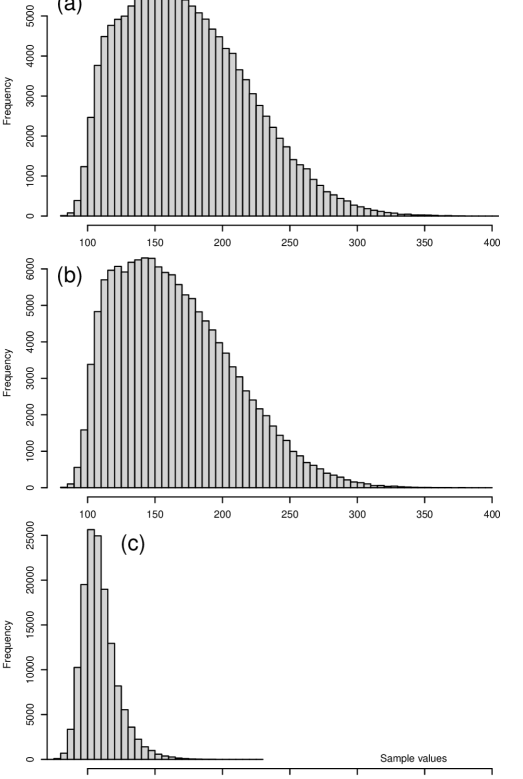
Figure 3: Perfect-sample histograms of the sum of absolute values of Bayesian Lasso regression coefficients, $T$, for different settings of the Lasso parameter $\lambda$: (a) $\lambda=0$, (b) $\lambda=0.237$, (c) $\lambda=5$.

6 Discussion

We have demonstrated perfect simulation for fairly general continuous distributions up to 100 dimensions. This greatly expands the range of problems to which perfect simulation can be applied. It also qualitatively improves MCMC convergence testing by removing the confounding between convergence and experimental error, which is present in all widely-used, existing tests of MCMC convergence. The MCMC practitioner using existing tests never knows whether convergence has been achieved. We have also introduced an objective measure of MCMC algorithm performance, in the number of likelihood derivative evaluations per perfect-sample point.

Our results confirm that Hamiltonian Monte Carlo is a very powerful method of MCMC and can be promoted over random-walk-based methods with their incumbent slow exploration of the sample space (see Neal, 2011, sec. 5.3.3). HMC is still not infallible: setting the time step is difficult when the variance is subject to radical change; e.g., the “funnel” example of Neal (2003, sec. 8). The need for transformation and reprogramming would, however, be evident from lack of coalescence.

HMC practice leads theory. Although its numerical results are outstanding, HMC does not produce an expression for the transition kernel, nor for the number of iterations that it takes to converge.

We ascribe the frequent superiority of the NUTS4 algorithm over FRUTS to its reliance on the initial HMC momentum vector to set the orientation of a trajectory. This feature stems from the original NUTS algorithm of Hoffman and Gelman (2014). FRUTS discards far fewer points than either NUTS or NUTS4 but orients its trajectories randomly, which appears to be a significant disadvantage.

Supplementary material

Extra text and figures:

Text and figures not included in body of paper. (PDF file)

R scripts:

R scripts for HMC and perfect sampling, with the diabetes data set used as an example. (ZIP file)

Journal submissions

We submitted an earlier version of this paper to the journal Annals of Statistics on 22 May 2020. It was rejected by the Editor without review but with complimentary comments. The reasons given for rejection were, “the contribution is purely computational” and “it lacks appeal to the general audience of the AOS and interested readers may also be able to find it more easily if it is published elsewhere”.

A similar version was submitted to Journal of Computational and Graphical Statistics (JCGS) on 8 June 2020. It was rejected with a recommendation for major revision, mainly in layout and style, on 10 March 2021 (first review period: nine months).

We extensively revised the paper, addressed all of the reviewers’ comments, and resubmitted it to JCGS on 13 September 2021. It was again rejected on 6 May 2022 (second review period: eight months). The reason given for rejection was that it contained a statement that the FRUTS algorithm ran “more efficiently” than the No U-Turn Sampler (NUTS), which we made on the basis that FRUTS had a much lower proportion of discarded trajectory points. The reviewer suggested that we either tone down that statement or provide a detailed comparison between FRUTS and NUTS. The Associate Editor requested that we provide the detailed comparison.

The first revision included a dedicated section on the recently developed technique of “unbiased simulation” in which there is much interest, and it showed that our methodology could easily accomplish unbiased simulation for general continuous problems, thereby greatly expanding the field of application of unbiased simulation. Nevertheless, the reviewer stated, “The question is whether a coupling scheme can be constructed to achieve perfect sampling. If such a scheme cannot be found, I really don’t see much point in doing this.”

We again extensively revised the paper to include the required comparison and address the reviewer’s comments. We comprehensively changed the paper’s coupling methods in favour of unbiased sampling over the older method of coupling from the past (CFTP), included new research showing how to derive perfect simulation from unbiased simulation, and presented perfect simulation in our results. We resubmitted to JCGS on 4 September 2022.

The paper was rejected by JCGS for the third and final time on 19 December 2022 (third review period: three and a half months; total review time with JCGS: twenty months; total elapsed time: two years and six months). The reason given for the final rejection was that the reviewer, the Associate Editor and the Editor all found the material “impenetrable”.

Supplementary material

S1 The full random uniform trajectory sampler

S1.1 Design

Algorithm S1 FRUTS trajectory for use in Algorithm 1: Setup and forward side

1:procedure Trajectory($q_{0},p_{0},r$) $\triangleright$ $r$: vector of random numbers, indexed by $[j]$

2:     $\triangleright$ Sample the direction vector $b$ uniformly from the surface of the unit sphere.

3:     $b\leftarrow$ UnitSphere($r[j_{\text{dir}}]$) $\triangleright$ $j_{\text{dir}}$: Indices of direction-vector random numbers

4:     $i^{+}\leftarrow i^{-}\leftarrow 0$; $q_{\text{traj}}[0,]\leftarrow q^{+}\leftarrow q^{-}\leftarrow q_{0}$ $\triangleright$ $q_{\text{traj}}[i^{-}:i^{+},]$ stores trajectory points.

5:     $p_{\text{traj}}[0,]\leftarrow p_{0}$; $\dot{p}_{0}\leftarrow-DU(q_{0})$ $\triangleright$ $p_{\text{traj}}[i^{-}:i^{+},]$ stores momentum.

6:     $p^{+}\leftarrow p_{0}^{+}\leftarrow p_{0}+{\scriptstyle\frac{1}{2}}\delta t\,\dot{p}_{0}$; $p^{-}\leftarrow p_{0}^{-}\leftarrow p_{0}-{\scriptstyle\frac{1}{2}}\delta t\,\dot{p}_{0}$ $\triangleright$ $p_{0}^{+},p_{0}^{-}$: half time-step offset of $p_{0}$

7:     $\triangleright$ If $b\cdot p_{0}^{+}$ and $b\cdot p_{0}^{-}$ have the same sign, construct two sides to the trajectory.

8:     $\triangleright$ Otherwise, construct the trajectory only on the side with the same sign as $b\cdot p_{0}$.

9:     $\triangleright$ On each constructed side, the leapfrog algorithm runs until $b\cdot p^{\pm}$ changes sign.

10:     if $\textbf{sgn}(b\cdot p_{0}^{+})\in\{\textbf{sgn}(b\cdot p_{0}^{-}),\textbf{sgn}(b\cdot p_{0})\}$ then $\triangleright$ Trajectory has a forward side.

11:         repeat

12:              $\dot{q}\leftarrow DK(p^{+})$; $q^{+}\leftarrow q^{+}+\delta t\,\dot{q}$ $\triangleright$ Hamiltonian dynamics

13:              $\dot{p}\leftarrow-DU(q^{+})$; $p^{+}\leftarrow p^{+}+\delta t\,\dot{p}$

14:              $\triangleright$ The final trajectory point, half-way along the segment over which the sign

15:              $\triangleright$ changes, is included only if it has the original sign of $b\cdot p_{0}^{+}$.

16:              if $\textbf{sgn}(b\cdot p^{+})=\textbf{sgn}(b\cdot p_{0}^{+})$ or $\textbf{sgn}(b\cdot(p^{+}-{\scriptstyle\frac{1}{2}}\delta t\,\dot{p}))=\textbf{sgn}(b\cdot p_{0}^{+})$ then

17:                  $i^{+}\leftarrow i^{+}+1$; $q_{\text{traj}}[i^{+},]\leftarrow q^{+}$; $p_{\text{traj}}[i^{+},]\leftarrow p^{+}-{\scriptstyle\frac{1}{2}}\delta t\,\dot{p}$ $\triangleright$ Store point.

18:              end if

19:         until $\textbf{sgn}(b\cdot p^{+})\neq\textbf{sgn}(b\cdot p_{0}^{+})$ $\triangleright$ Test for change of sign.

20:     end if$\triangleright$ Algorithm continues below

Algorithm S2 FRUTS trajectory: Backward side and selection of destination point

21:     if $\textbf{sgn}(b\cdot p_{0}^{-})\in\{\textbf{sgn}(b\cdot p_{0}^{+}),\textbf{sgn}(b\cdot p_{0})\}$ then $\triangleright$ Trajectory has a backward side.

22:         repeat

23:              $\dot{q}\leftarrow DK(p^{-})$; $q^{-}\leftarrow q^{-}-\delta t\,\dot{q}$ $\triangleright$ Hamiltonian dynamics

24:              $\dot{p}\leftarrow-DU(q^{-})$; $p^{-}\leftarrow p^{-}-\delta t\,\dot{p}$

25:              $\triangleright$ Include the final trajectory point only if it has the original sign of $b\cdot p_{0}^{-}$.

26:              if $\textbf{sgn}(b\cdot p^{-})=\textbf{sgn}(b\cdot p_{0}^{-})$ or $\textbf{sgn}(b\cdot(p^{-}+{\scriptstyle\frac{1}{2}}\delta t\,\dot{p}))=\textbf{sgn}(b\cdot p_{0}^{-})$ then

27:                  $i^{-}\leftarrow i^{-}-1$; $q_{\text{traj}}[i^{-},]\leftarrow q^{-}$; $p_{\text{traj}}[i^{-},]\leftarrow p^{-}+{\scriptstyle\frac{1}{2}}\delta t\,\dot{p}$ $\triangleright$ Store point.

28:              end if

29:         until $\textbf{sgn}(b\cdot p^{-})\neq\textbf{sgn}(b\cdot p_{0}^{-})$ $\triangleright$ Test for change of sign.

30:     end if

31:     $n_{\text{pt}}\leftarrow i^{+}-i^{-}+1$ $\triangleright$ Number of points in trajectory; note $i^{-}\leq 0$.

32:     $\triangleright$ Select the destination randomly and uniformly from the set of trajectory points.

33:     if $b\cdot q_{\text{traj}}[i^{-},]\leq b\cdot q_{\text{traj}}[i^{+},]$ then $\triangleright$ Order trajectory points by $b\cdot q$; see Fig. 1.

34:         $i_{\text{dest}}\leftarrow i^{-}+\textbf{floor}(n_{\text{pt}}\times r[j_{\text{sel}}])$ $\triangleright$ $r[j_{\text{sel}}]$: $U(0,1)$ variate to select destination

35:     else

36:         $i_{\text{dest}}\leftarrow i^{+}-\textbf{floor}(n_{\text{pt}}\times r[j_{\text{sel}}])$ $\triangleright$ Reverse order compared to above.

37:     end if

38:     return $(q_{\text{traj}}[i_{\text{dest}},],p_{\text{traj}}[i_{\text{dest}},])$

39:end procedure

The FRUTS algorithm (Algorithm S1) is conceptually simpler than NUTS and better samples the full trajectory, as it includes all the eligible points up to the U-turns, rather than discarding up to half of them. Its major innovation is to choose, independently of the trajectory generation, a direction vector $b$ for each trajectory, whose dot products with trajectory increments must not change sign. We sample $b$ randomly and uniformly from the surface of the $d$-dimensional unit sphere, independently for each trajectory.

Limiting the number of points in a trajectory, to bound the storage space and execution time in case the time step is too small or the target distribution has longer tails than expected, is explained in section S1.3.

Our coding of FRUTS numbers the trajectory points in the order of their dot products with the direction vector, not in the order of increasing time as stated in section 2.4 and Figure 1 of the paper. We believed that this ordering was more logical given the reliance of the algorithm on the direction vector, but it makes no practical difference to the operation of the algorithm.

S1.2 Proof of detailed balance

The general principles by which HMC leapfrog algorithms satisfy detailed balance were set out by Duane et al. (1987) (see section 2.1). From those principles, Hoffman and Gelman (2014, section 3.1.1) established detailed balance for NUTS by proving that the set, denoted $\mathcal{C}$, of discrete points $(q,p)$ in a trajectory is invariant to the choice of trajectory origin within $\mathcal{C}$. In other words, from a discretized trajectory $\mathcal{C}$ generated by the algorithm, choose any pair ($q_{0}$, $p_{0}$) as origin and initial momentum vector of a trajectory, and generate a new trajectory $\mathcal{C}^{\prime}$. Then an HMC algorithm that selects its destination point as $(q,p)\in_{R}\mathcal{C}$, i.e., randomly and uniformly from $\mathcal{C}$, which both NUTS and FRUTS do, satisfies detailed balance if $\mathcal{C}^{\prime}=\mathcal{C}$ for every choice ($q_{0}$, $p_{0}$) $\in\mathcal{C}$.

We show that FRUTS satisfies the invariance condition $\mathcal{C}^{\prime}=\mathcal{C}$ for detailed balance.

The momentum vectors $p^{+}$ and $p^{-}$ at integer-plus-a-half time steps are derived from $p_{0}$ by the derivative $\dot{p}$ evaluated at integer time steps, according to (2) and lines 6, 13 and 24 of Algorithm S1. The reversibility of both HMC and the leapfrog algorithm (see section 2.1) proves that $p^{+}$, $p^{-}$ and all pairs ($q$, $p$) $\in\mathcal{C}$ are reproduced, no matter which pair is selected as the origin. The proof that $\mathcal{C}^{\prime}=\mathcal{C}$ then rests on the FRUTS stopping and starting rules on the forward and backward sides of the trajectory, which determine exactly which of the discrete trajectory points belong to $\mathcal{C}$ and $\mathcal{C}^{\prime}$.

When $q_{0}$ is an internal point, not an endpoint of $\mathcal{C}$, the reproduction of trajectory points proves that $\mathcal{C}^{\prime}=\mathcal{C}$ whatever the choice of internal $q_{0}$, because the forward and backward endpoint stopping rules, determined by the trajectory points, do not depend on this choice. The same argument applies when $q_{0}$ is an endpoint of $\mathcal{C}$ at which $\text{sgn}(b\cdot p_{0}^{+})=\text{sgn}(b\cdot p_{0}^{-})$. In that case the following trajectory point $(q_{X},p_{X})$ must have triggered the stopping rule when $\mathcal{C}$ was constructed, and been excluded from $\mathcal{C}$ because $\text{sgn}(b\cdot p_{X})\neq\text{sgn}(b\cdot p_{0}^{\pm})$. That point will likewise be excluded from $\mathcal{C}^{\prime}$.

The remaining case is when $q_{0}$ is an endpoint of $\mathcal{C}$ and $\text{sgn}(b\cdot p_{0}^{+})\neq\text{sgn}(b\cdot p_{0}^{-})$. Then the FRUTS rule for starting a trajectory specifies that $\mathcal{C}^{\prime}$ is generated only on the side with $\text{sgn}(b\cdot p)=\text{sgn}(b\cdot p_{0})$. Thus $q_{0}$ is also an endpoint of $\mathcal{C}^{\prime}$. Furthermore, by the FRUTS stopping rule, if $\mathcal{C}$ originated from a point other than $q_{0}$ , $q_{0}\in\mathcal{C}$ could only have occurred if $q_{0}$ was approached from the side on which $\text{sgn}(b\cdot p_{0}^{\pm})=\text{sgn}(b\cdot p_{0})$ ; i.e., the side on which $\mathcal{C}^{\prime}$ is constructed. Again the reproduction of trajectory points ensures that $\mathcal{C}^{\prime}=\mathcal{C}$.

S1.3 Limiting the number of trajectory sample points

This section describes an additional feature of the design of the Full Random Uniform Trajectory Sampler (FRUTS), presented in section 3.1 of the paper.

We impose an initial limit $N$ on the number of points on either side of a trajectory, allowing up to $2N+1$ points over the positive and negative sides combined. Our hope, however, is that the combination of the time-step setting and the dot-product conditions of the FRUTS algorithm will cause both sides of the trajectory to terminate well below this limit.

If the dot-product termination condition is encountered on both sides of the trajectory within the initial limit of $N$ points per side, the FRUTS algorithm is unaltered.

If the condition is encountered on only one side, we extend the other side until it either terminates or would exceed the limit of $2N+1$ points in total, both sides combined. If it terminates, the FRUTS algorithm is again unaltered. If it doesn’t terminate, we sample from the collection of all the points on the first side but only the first $N$ points on the second side. For each point other than the origin $O$, the probability of selecting that point is set at $1/(2N+1)$ and the balance of the probability is assigned to $O$ so that the probabilities sum to 1. This rule can confer a substantial probability (worst case slightly more than 0.5) of staying in the same place by choosing the destination $P$ to equal $O$, but is necessary for detailed balance.

If neither side encounters the termination condition, the set of $2N+1$ points ($N$ on each side) is used and each point is given equal probability $1/(2N+1)$ of being selected as the destination $P$.

Detailed balance is satisfied because the Markov transition matrix for the set of all points on the maximal trajectory from the unadjusted FRUTS algorithm is doubly stochastic: all rows and also all columns sum to 1. Therefore its stationary distribution is uniform (see, e.g., Pinsky and Karlin, 2011, sec. 4.1.1), which is the condition for detailed balance.

The doubly stochastic nature of the transition matrices and the change in formulation when the trajectory is longer than $2N+1$ points are illustrated in Figure S1.

Figure S1: Markov transition matrices showing implementation of an artificial limit on the number of trajectory points, to limit storage space and execution time in case the time step has been chosen too small or the target distribution is unexpectedly long-tailed. Here the limit is $2N+1$ = 5 points, and the whole trajectory consists of either (a) 5 or (b) 6 points. In (a), the limit fits within the full length of the trajectory, and the destination is selected from a discrete uniform distribution. In (b), the trajectory contains more points than the limit: then a maximum of $N=2$ points on each side of the origin is allowed. Both matrices are doubly stochastic, so have uniform stationary distribution and thereby satisfy detailed balance.

S2 Setting the time step

For convenience, we reproduce two equations from the main paper here: the kinetic energy equation

$$K=|p|^{\beta}/\beta$$ (S1)

and the velocity equation

$$\dot{q}=\left(dK/{d|p|}\right)p/|p|=|p|^{\beta-2}p.$$ (S2)

We assume that the location coordinates $q$ are scaled to make the variance of $q$ approximately equal to the identity matrix; e.g., by first optimizing to find the maximum-likelihood point, then scaling by the square-root of the Hessian matrix at that point. Such a procedure is used in, e.g., the software AD Model Builder (Fournier et al., 2011).

Similarly to equation (S1) for kinetic energy, for the purpose of setting the time step we approximate the potential energy (negative log-likelihood) by the form

$$U=|q^{\alpha}|/\alpha,\quad|q|=(\alpha U)^{1/\alpha}.$$ (S3)

The case $\alpha=2$ corresponds to a normal distribution. Values $\alpha<2$ can be used if the target distribution is long-tailed (e.g., our $t$-distribution example). The form (S3) calibrates the negative log-likelihood to be zero at the maximum-likelihood point.

The boundary of the region in $q$-space that a trajectory with Hamiltonian value $H$ can traverse is hit when $U=H$ and $K=0$; i.e., maximum potential and minimum kinetic energy. This region has diameter, from (S3),

$$D=2(\alpha H)^{1/\alpha}.$$ (S4)

The speed of the HMC particle on its trajectory is, by (S2),

$$|\dot{q}|=|p|^{\beta-1}=(\beta K)^{1-1/\beta}=(\beta H)^{1-1/\beta}(K/H)^{1-1/\beta}.$$ (S5)

By (S1) and (S3), incorporating the surface area of a $d$-dimensional sphere, the densities of $|p|$ and $|q|$ are proportional to $|p|^{d-1}\exp\big{(}-|p|^{\beta}/\beta\big{)}$ and $|q|^{d-1}\exp\big{(}-|q|^{\alpha}/\alpha\big{)}$ respectively. Transforming back to the variables $K$ and $U$, the density of $K$ is proportional to ($K>0$)

$$|p|^{d-1}\exp{(-|p|^{\beta}/\beta)}\big{/}{(dK/d|p|)}=|p|^{d-\beta}\exp(-|p|^{\beta}/\beta)\propto K^{d/\beta-1}\exp(-K),$$

a gamma distribution with shape parameter $d/\beta$ and rate parameter 1. Similarly, $U$ has an independent gamma distribution with shape parameter $d/\alpha$ and rate parameter 1.

Returning to (S5) and using properties of the gamma and beta distributions (see, e.g., Encyclopedia of Mathematics, 2020), the distributions of $H=U+K$ and $K/H$ are, independently, gamma with shape $d/\beta+d/\alpha$ and beta with parameters ($d/\beta$, $d/\alpha$). The expectation of $|\dot{q}|$ conditional on $H$ is

$$E\big{(}|\dot{q}|\,\big{|}\,H\big{)} =(\beta H)^{1-1/\beta}\,\frac{\Gamma(d/\beta+d/\alpha)}{\Gamma(d/\beta)\,\Gamma(d/\alpha)}\int_{0}^{1}x^{1-1/\beta}x^{d/\beta-1}(1-x)^{d/\alpha-1}\,dx$$

$$=(\beta H)^{1-1/\beta}\,\frac{\Gamma(d/\beta+1-1/\beta)\,\Gamma(d/\beta+d/\alpha)}{\Gamma(d/\beta)\,\Gamma(d/\beta+d/\alpha+1-1/\beta)}\,.$$

Let $h$ be the reciprocal of the number of points desired in a trajectory. Then, still conditional on $H$ and using (S4), the time step $\delta t$ can be set to

$$\delta t=hD/{E\left(|\dot{q}|\,\big{|}\,H\right)}=2h(\alpha H)^{1/\alpha}(\beta H)^{1/\beta-1}\frac{\Gamma(d/\beta)\,\Gamma(d/\beta+d/\alpha+1-1/\beta)}{\Gamma(d/\beta+1-1/\beta)\,\Gamma(d/\beta+d/\alpha)}\,.$$ (S6)

If $\alpha=\beta=2$, this does not depend on $H$ and it can be expected that the number of trajectory points will vary little between trajectories. For general $\alpha$ and $\beta$, which may be needed for long-tailed distributions, we use (S6) with the gamma distribution of $H$ to find

$$E(1/\delta t)=\frac{\beta^{1-1/\beta}\alpha^{-1/\alpha}\Gamma(d/\beta+1-1/\beta)}{2h\Gamma(d/\beta)\,\Gamma(d/\beta+d/\alpha+1-1/\beta)}\int_{0}^{\infty}H^{1-1/\beta-1/\alpha}H^{d/\beta+d/\alpha-1}e^{-H}\,dH.$$

The integral is another gamma function and taking reciprocals yields the final time step:

$$\delta t=2h\beta^{1/\beta-1}\alpha^{1/\alpha}\,\frac{\Gamma(d/\beta)}{\Gamma\big{(}\{d-1\}/\beta+1\big{)}}\cdot\frac{\Gamma\big{(}\{d-1\}/\beta+d/\alpha+1\big{)}}{\Gamma\big{(}\{d-1\}/\beta+\{d-1\}/\alpha+1\big{)}}\,.$$ (S7)

S3 CFTP and ROCFTP algorithms

Algorithm S3 Coupling from the past, calling HMC with rounding (Algorithm 3)

1:procedure CFTP($n_{\text{st}},Q_{0},n_{\text{it}},N_{\text{it}},R,r_{\text{ro}},w$) $\triangleright$ $n_{\text{st}},Q_{0}$: number and matrix of starting

2:$\triangleright$ points; $n_{\text{it}},N_{\text{it}}$: number and maximum allowed number of iterations (trajectories)

3:     $Q\leftarrow Q_{0}$; $n_{\text{coal}}\leftarrow 1$ $\triangleright$ Matrix to hold results; number of coalesced results

4:     for $i_{\text{st}}\leftarrow 1:n_{\text{st}}$ do $\triangleright$ Loop over different starting points.

5:         $\triangleright$ Use same random numbers $R$ for each starting point; always end at row $N_{\text{it}}$.

6:         $Q[i_{\text{st}},]\leftarrow$ HmcRound($Q[i_{\text{st}},],n_{\text{it}},R[(N_{\text{it}}-n_{\text{it}}+1):N_{\text{it}},],r_{\text{ro}},w$)

7:         if $i_{\text{st}}\geq 2$ and $Q[i_{\text{st}},]=Q[i_{\text{st}}-1,]$ then $\triangleright$ Count coalesced outcomes.

8:              $n_{\text{coal}}\leftarrow n_{\text{coal}}+1$ $\triangleright$ Increment when same as from previous starting point.

9:         end if

10:     end for

11:     return $(Q,n_{\text{coal}})$ $\triangleright$ Increase $n_{\text{it}}$ and rerun until all coalesced ($n_{\text{coal}}=n_{\text{st}}$).

12:end procedure

Algorithm S4 Read-once coupling from the past (ROCFTP) (adjusted Algorithm S3)

1:procedure ROCFTP($n_{\text{st}},Q_{0},n_{\text{it}},N_{S},d_{R},w$) $\triangleright$ $n_{\text{st}},Q_{0}$: number and matrix of starting

2:$\triangleright$ points; $n_{\text{it}}$: block length (number of trajectories); $N_{S}$: required sample size;

3:$\triangleright$ $d_{R}$: number of random numbers per trajectory; $w$: rounding width

4:     $Q\leftarrow\textbf{zeros}(n_{\text{st}}+1,d)$; $Q_{S}\leftarrow\textbf{zeros}(N_{S},d)$ $\triangleright$ Storage for current and final results

5:     $Q[n_{\text{st}}+1,]=Q_{0}[n_{\text{st}},]$ $\triangleright$ Initialize the final-result row; don’t reset during blocks.

6:     $i_{S}=0$ $\triangleright$ Set final-result counter; need one coalesced block before we store any.

7:     repeat

8:         $Q_{S}[\max(i_{S},1),]=Q[n_{\text{st}}+1,]$ $\triangleright$ Store initial value in case this block coalesces.

9:         $R\leftarrow\textbf{rand}(n_{\text{it}},d_{R})$ $\triangleright$ Generate random numbers for HMC, dimensions $n_{\text{it}}\times d_{R}$.

10:         $r_{\text{ro}}\leftarrow\textbf{rand}(d+1)$ $\triangleright$ Generate random numbers for rounding, dimension $d+1$.

11:         $Q[1:n_{\text{st}},]\leftarrow Q_{0}$; $n_{\text{coal}}\leftarrow 1$ $\triangleright$ Initialize block and number of coalesced results.

12:         for $i_{\text{st}}\leftarrow 1:n_{\text{st}}+1$ do $\triangleright$ Loop over different starting points.

13:              $Q[i_{\text{st}},]\leftarrow$ HmcRound($Q[i_{\text{st}},],n_{\text{it}},R,r_{\text{ro}},w$)

14:              if $i_{\text{st}}\geq 2$ and $i_{\text{st}}\leq n_{\text{st}}$ and $Q[i_{\text{st}},]=Q[i_{\text{st}}-1,]$ then

15:                  $n_{\text{coal}}\leftarrow n_{\text{coal}}+1$ $\triangleright$ Count coalesced outcomes (where same as previous).

16:              end if

17:         end for

18:         if $n_{\text{coal}}=n_{\text{st}}$ then $\triangleright$ Test coalescence (same results from all starting points).

19:              $i_{S}=i_{S}+1$ $\triangleright$ One final result per coalesced block, after the first one

20:         end if

21:     until $i_{S}>N_{S}$

22:     return $Q_{S}$

23:end procedure

S4 Results for NUTS and Raw HMC

Table S1: Perfect simulation results for standard distributions with the NUTS and Raw HMC algorithms. Symbol $d$ is number of dimensions, $\rho$ is pairwise correlation coefficient (aspect ratio of variance ellipsoid in parentheses), $\nu$ is degrees of freedom, $\alpha$ is the distribution-tail parameter (noted when $\alpha\neq 2$), and $\mu$ is the nonzero mode. Perfect-sample size is listed (number of independent sample sets in parentheses, k denotes 1000), then numbers of likelihood-derivative evaluations per perfect sample point for the NUTS and Raw HMC algorithms (dash indicates not conducted), and the maximum number of blocks for coalescence of chains in Algorithm 4 of the paper (bold indicates problem cases).

Name	$d$	Parameters set	Sample	NUTS	Raw	Max
Standard normal	1	–	140k (10k)	914	300	3
	10	–	14k (1k)	1350	521	3
	100	–	14k (1k)	1439	642	2
Correlated normal	2	$\rho=0.6$ (4)	14k (1k)	1738	652	3
		$\rho=0.95$ (39)	14k (1k)	–	841	3
	100	$\rho=0.45$ (82.82)	280 (20)	42222	–	2
$t$-distribution	1	$\nu=4$	14k (1k)	1118	1092	12
	10	$\nu=4$, $\alpha=1.5$	14k (1k)	4756	5047	7
	100	$\nu=4$, $\alpha=1.25$	14k (1k)	32361	–	5
Normal mixture	1	$\mu=4$	14k (1k)	–	1222	4
		$\mu=6$	2.8k (200)	6396	9550	5
	10	$\mu=6$	1.4k (100)	–	12046	6
	100	$\mu=6$	280 (20)	13908	–	4

S5 Histograms of the residual sum of squares in the Bayesian Lasso

This section presents and describes the histograms of the residual sum of squares, mentioned in section 5 of the paper.

Histograms of the residual sum of squares, $S$, are shown in Figure S2, for $\lambda=0$ (no Lasso term), 0.237 and 5.

The distributions of $S$ for $\lambda=0$ and $\lambda=0.237$ are practically indistinguishable. The one for $\lambda=5$ shows a slight shift towards larger values of $S$; i.e., slightly worse fit of the linear regression. The mean values of $S/1000$ are 1295.65, 1295.52 and 1298.76 for $\lambda=0$, 0.237 and 5 respectively.

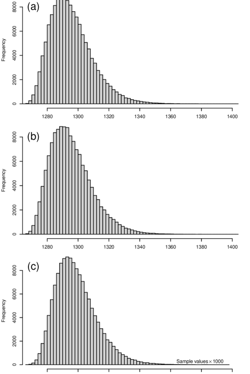
Figure S2: Perfect-sample histograms of the residual sum of squares for the Bayesian Lasso, $S$, for different settings of the Lasso parameter $\lambda$: (a) $\lambda=0$, (b) $\lambda=0.237$, (c) $\lambda=5$.

References

- Aldous and Diaconis (1987) Aldous, D. and P. Diaconis (1987, March). Strong uniform times and finite random walks. Adv. Appl. Math. 8(1), 69–97.
- Bellman (1955) Bellman, R. (1955). Review of Transactions of the Symposium on Computing, Mechanics, Statistics, and Partial Differential Equations, Volume II. J. Amer. Statist. Assoc. 50(272), 1357–1359.
- Botev et al. (2018) Botev, Z., Y.-L. Chen, P. L’Ecuyer, S. MacNamara, and D. P. Kroese (2018, December). Exact posterior simulation from the linear LASSO regression. In Proc. 2018 Winter Simul. Conf., Gothenburg, pp. 1706–1717. ACM.
- Carpenter et al. (2017) Carpenter, B., A. Gelman, M. D. Hoffman, D. Lee, B. Goodrich, M. Betancourt, M. Brubaker, J. Guo, P. Li, and A. Riddell (2017). Stan: A probabilistic programming language. J. Statist. Softw. 76(1), doi:10.18637/jss.v076.i01.
- Craiu and Meng (2011) Craiu, R. V. and X.-L. Meng (2011, May). Perfection within reach: Exact MCMC sampling. In S. Brooks, A. Gelman, G. Jones, and X.-L. Meng (Eds.), Handbook of Markov Chain Monte Carlo, pp. 199–226. Chapman and Hall.
- Duane et al. (1987) Duane, S., A. D. Kennedy, B. J. Pendleton, and D. Roweth (1987, September). Hybrid Monte Carlo. Phys. Lett. B 195(2), 216–222.
- Efron et al. (2004) Efron, B., T. Hastie, L. Johnstone, and R. Tibshirani (2004). Least angle regression. Ann. Statist. 32, 407–499.
- Encyclopedia of Mathematics (2020) Encyclopedia of Mathematics (2020). Gamma-distribution. In Encyclopedia of Mathematics. EMS Press, encyclopediaofmath.org.
- Fill (1998) Fill, J. A. (1998). An interruptible algorithm for perfect sampling via Markov chains. Ann. Appl. Probab. 8(1), 131–162.
- Fournier et al. (2011) Fournier, D. A., H. J. Skaug, J. Ancheta, J. Ianelli, A. Magnusson, M. N. Maunder, A. Nielsen, and J. Sibert (2011, October). AD Model Builder: Using automatic differentiation for statistical inference of highly parameterized complex nonlinear models. Optim. Methods Softw. 27(2), DOI: 10.1080/10556788.2011.597854.
- Gelman and Rubin (1992) Gelman, A. and D. B. Rubin (1992, November). Inference from iterative simulation using multiple sequences. Statist. Sci. 7(4), 457–472.
- Gelman and Shirley (2011) Gelman, A. and K. Shirley (2011, May). Inference and monitoring convergence. In S. Brooks, A. Gelman, G. Jones, and X.-L. Meng (Eds.), Handbook of Markov Chain Monte Carlo, pp. 163–174. Chapman and Hall.
- Glynn and Rhee (2014) Glynn, P. W. and C.-H. Rhee (2014, December). Exact estimation for Markov chain equilibrium expectations. Journal of Applied Probability 51(A), 377–389.
- Hamilton (1834) Hamilton, W. R. (1834). On a general method in dynamics; by which the study of the motions of all free systems of attracting or repelling points is reduced to the search and differentiation of one central relation, or characteristic function. Philos. Trans. Roy. Soc. 124, 247–308.
- Hamilton (1835) Hamilton, W. R. (1835). Second essay on a general method in dynamics. Philos. Trans. Roy. Soc. 125, 95–144.
- Hastings (1970) Hastings, W. K. (1970). Monte Carlo sampling methods using Markov chains and their applications. Biometrika 57(1), 97–109.
- Hoffman and Gelman (2014) Hoffman, M. D. and A. Gelman (2014). The No-U-Turn Sampler: Adaptively setting path lengths in Hamiltonian Monte Carlo. J. Mach. Learn. Res. 15, 1593–1623.
- Huber (2016) Huber, M. L. (2016). Perfect Simulation. Boca Raton, FL: CRC Press.
- Jacob et al. (2020) Jacob, P. E., J. O’Leary, and Y. F. Atchadé (2020). Unbiased Markov chain Monte Carlo methods with couplings. Journal of the Royal Statistical Society: Series B (Statistical Methodology) 82(3), 543–600.
- Kroese et al. (2014) Kroese, D. P., T. Brereton, T. Taimre, and Z. I. Botev (2014). Why the Monte Carlo method is so important today. WIREs Comput. Statist. 6(6), 386–392.
- Lovász and Winkler (1995) Lovász, L. and P. Winkler (1995). Exact mixing in an unknown Markov chain. The Electronic Journal of Combinatorics 2, article R15.
- Metropolis et al. (1953) Metropolis, N., A. W. Rosenbluth, M. N. Rosenbluth, A. H. Teller, and E. Teller (1953). Equations of state calculations by fast computing machines. J. Chem. Phys. 21, 1087–1092.
- Mira et al. (2001) Mira, A., J. Møller, and G. O. Roberts (2001). Perfect slice samplers. J. R. Stat. Soc. Ser. B. Stat. Methodol. 63(3), 593–606.
- Murdoch and Green (1998) Murdoch, D. J. and P. J. Green (1998). Exact sampling from a continuous state space. Scand. J. Stat. 25(3), 483–502.
- Neal (1993) Neal, R. M. (1993). Probabilistic Inference Using Markov Chain Monte Carlo Methods. Research report, Department of Computer Science, University of Toronto.
- Neal (1995) Neal, R. M. (1995). Bayesian Learning for Neural Networks. PhD thesis, University of Toronto, Graduate Department of Computer Science.
- Neal (2003) Neal, R. M. (2003, June). Slice sampling. Ann. Statist. 31(3), 705–767.
- Neal (2011) Neal, R. M. (2011, May). MCMC using Hamiltonian dynamics. In S. Brooks, A. Gelman, G. Jones, and X.-L. Meng (Eds.), Handbook of Markov Chain Monte Carlo, pp. 113–162. Chapman and Hall.
- Park and Casella (2008) Park, T. and G. Casella (2008, June). The Bayesian Lasso. J. Amer. Statist. Assoc. 103(482), 681–686.
- Pinsky and Karlin (2011) Pinsky, M. A. and S. Karlin (2011, January). An Introduction to Stochastic Modeling (Fourth Edition). Boston: Academic Press.
- Propp and Wilson (1996) Propp, J. G. and D. B. Wilson (1996). Exact sampling with coupled Markov chains and applications to statistical mechanics. Random Structures Algorithms 9(1–2), 223–252.
- R Core Team (2022) R Core Team (2022). R: A language and environment for statistical computing. Vienna: R Foundation for Statistical Computing.
- Roy (2020) Roy, V. (2020, March). Convergence diagnostics for Markov chain Monte Carlo. Annu. Rev. Stat. Appl. 7, 387–412.
- Sutradhar (2006) Sutradhar, B. C. (2006). Multivariate t-distribution. In Encyclopedia of Statistical Sciences. Wylie.
- Tibshirani (1996) Tibshirani, R. (1996). Regression shrinkage and selection via the Lasso. J. R. Stat. Soc. Ser. B. Stat. Methodol. 58(1), 267–288.
- Wilson (2000) Wilson, D. B. (2000). How to couple from the past using a read-once source of randomness. Random Structures Algorithms 16(1), 85–113.