Bridging the Domain Gap in Satellite Pose Estimation: a Self-Training Approach based on Geometrical Constraints

Abstract

Recently, unsupervised domain adaptation in satellite pose estimation has gained increasing attention, aiming at alleviating the annotation cost for training deep models. To this end, we propose a self-training framework based on the domain-agnostic geometrical constraints. Specifically, we train a neural network to predict the 2D keypoints of a satellite and then use PnP to estimate the pose. The poses of target samples are regarded as latent variables to formulate the task as a minimization problem. Furthermore, we leverage fine-grained segmentation to tackle the information loss issue caused by abstracting the satellite as sparse keypoints. Finally, we iteratively solve the minimization problem in two steps: pseudo-label generation and network training. Experimental results show that our method adapts well to the target domain. Moreover, our method won the 1st place on the sunlamp task of the second international Satellite Pose Estimation Competition.

I INTRODUCTION

Estimating the pose of an uncooperative spacecraft is crucial in numerous space missions, such as debris removal [1], on-orbit servicing [2], and assets refueling [3]. In the last two decades, numerous relative navigation systems have been proposed based on LiDARs [4, 5] and cameras [6, 7, 8, 9, 10, 11]. Active sensors, including radars and LiDARs, requires larger mass and higher power consumption compared to visual sensors. Moreover, a stereo system requires a large baseline and relies on robust feature matching to obtain depth information. Therefore, monocular vision based navigation systems have gained increasing attention from the academical and industrial fields.

Traditionally, monocular satellite pose estimation approaches require hand-crafted feature extraction [6, 7, 8, 9], which limits their performance on challenging environments, such as occlusions, harsh lighting conditions, reflective materials, and complex structures. Recently, deep learning based methods have achieved success in satellite pose estimation [11], thanks to the powerful feature representation ability of deep models. However, training neural networks requires large-scale datasets, while collecting real images of spacecrafts and annotating their 6-DoF poses are time-consuming, notoriously laborious, and difficult. Therefore, recent deep models are trained and evaluated using synthetic images [12, 13, 14, 11, 15]. Due to the inherent discrepancy between real and synthetic images, the deep models that are fully-supervised by synthetic images usually show deteriorated performance when being deployed in real scenarios. This issue is revealed by the large gap between scores on the real and synthetic leaderboards.

In computer vision, unsupervised domain adaptation (UDA) [16, 17, 18, 19, 20, 21] is adopted in scenarios where the labels of real samples are scarce, by training deep models using labeled synthetic images and unlabeled real images. Motivated by these practices, Park et al. [22] created the next generation spacecraft pose estimation dataset (SPEED+) with focus on the synthetic-to-real domain gap in satellite pose estimation. Moreover, based on the SPEED+ dataset, the Advanced Concepts Team (ACT) of the European Space Agency (ESA) and the Space Rendezvous Laboratory (SLAB) at Stanford University co-organized the second international Satellite Pose Estimation Competition (SPEC2021) to boost the research of bridging the domain gap.

Different to common UDA tasks in computer vision, a calibrated camera is used to measure the pose of the same satellite under various environments in space missions. For UDA in satellite pose estimation in SPEC2021, only the environmental settings are different across domains while the satellite structure and the camera parameters are the same (as shown in Fig. 1). Therefore, given a pose, the locations of keypoints and the satellite masks are the same in different domains, which are referred to as the domain-agnostic geometrical constraints. Besides, due to intense imaging noise, challenging illumination variations, and diverse poses, this task poses additional challenges compared with common UDA problems [17, 19, 18].

(a) synthetic

(b) lightbox

(c) sunlamp

Figure 1: The characteristic of the UDA task in satellite pose estimation. The satellite structures are the same in different domains with different illumination conditions. The samples come from three distinct domains, including synthetic (well illuminated), lightbox (low contrast, highly noisy), and sunlamp (specular reflection). Top: the original images from [22] with the 2D keypoints and the reprojected wireframe model. Bottom: the fine-grained masks. Note that, the visualization results on the synthetic image is obtained using the ground-truth pose, while the poses used on the lightbox and sunlamp images are predicted by our network.

Several UDA approaches [23, 24, 25, 20, 21, 26] have been proposed to explore self-training paradigms to improve performance on the target domain. Nonetheless, these methods are not specifically designed for UDA in satellite pose estimation, since the domain-agnostic geometrical constraints are not fully explored. Meanwhile, previous satellite pose estimation approaches [12, 15] represent a satellite as a set of 2D keypoints, and then estimate the satellite pose using the perspective-n-point (PnP) algorithms [27]. However, as shown in Fig. 1, sparse keypoints stand for only semantic parts of the satellite. Such sparse representation leads to a significant loss of information, which hampers knowledge transfer across domains.

To tackle the above problems, we formulate UDA of satellite pose estimation as a minimization problem under a self-training framework. First, we formulate the geometrical constraints as a projection function, which maps the predefined 3D keypoints onto the source and target images using the same camera parameters. Based on the projection function, we propose a basic self-training framework by taking the poses of target samples as latent variables, which are jointly optimized with the network parameters. Second, we leverage fine-grained segmentation to extend the basic framework. Specifically, we enhance the geometrical constraints with a rendering function. Similar to the projection function, the rendering function maps the 3D mesh of the satellite to fine-grained masks, using the same camera parameters in different domains. Therefore, we take fine-grained segmentation as an auxiliary task of keypoints regression. Furthermore, as the masks provide dense descriptions with structural information, we perform adversarial training by aligning the predicted masks of the source and target samples. Finally, we iteratively optimize the network parameters and generate pseudo labels to solve the minimization problem. Experimental results demonstrate the effectiveness of our framework. Moreover, our method won the 1st and the 3rd place on two leaderboards of the second international Satellite Pose Estimation Competition, respectively.

Our contributions can be summarized as follows: (1) We explore the domain-agnostic geometrical constraints to propose a self-training framework for UDA in satellite pose estimation. (2) We leverage fine-grained masks to address the information loss problem caused by abstracting the satellite as sparse keypoints. (3) Our method significantly improves the accuracy of satellite pose estimation without using real annotations.

II RELATED WORK

Object pose estimation aims at recovering the 3D position and 3D rotation of an object in the camera-centered coordinate system. Traditional approaches [28, 29] rely on local features, suffering from texture-less objects and background clutter. Recently, CNN-based methods have dominated most object pose estimation tasks. Numerous approaches [30, 31, 32, 33, 34, 35] have been proposed to estimate poses using putative 2D-3D correspondences and the PnP algorithms. To achieve better efficiency, several methods [36, 37, 38, 39] are introduced to directly regress poses from monocular images. Other methods [40, 41, 42] learn the latent representations of rotation and recover poses by exploring the image retrieval paradigms. Since these methods focus on household objects in indoor scenarios [43, 44], they face significant challenges caused by wide-range depth variations and illumination changes in outer space [45].

Satellite pose estimation is a special case of object pose estimation. Spacecraft Pose Network (SPN) [14] is the first deep learning-based approach for satellite pose estimation. Specifically, the 3D rotation is recovered by discretizing the viewpoint spaces into bins, and then the 3D translation is estimated using the geometrical constraints. In other top-performing approaches, the pose estimation problem is formulated as a task of localizing semantic keypoints on the convex areas of a satellite by taking various representations, such as heatmap [12], vector [13], and set [15]. These methods crop the satellite from the input images using a well-trained object detector to address scale variations. To achieve better efficiency, Hu et al [45] handle the scale problem in a single-stage way by introducing a sampling strategy. However, these methods are trained and tested on synthetic data. They usually undergo significant performance degradation when being applied to real images due to the domain gap [46].

Unsupervised domain adaptation aims at addressing the domain mismatch problem. It is a promising direction to circumvent the laborious and time-consuming procedures of data annotation. Several UDA paradigms have been studied for different vision tasks. Adversarial learning aligns both domains with a discriminator. The alignment can be achieved at image-level [16], feature-level [17, 18], and output-level [19]. Self-training methods are introduced to utilize target samples to train the model by generating pseudo labels [23, 24], minimizing the entropy loss [25, 20], or employing the teacher-student framework [21, 26]. Nonetheless, it is challenging to adopt these approaches in UDA of satellite pose estimation, which is different to the common UDA tasks in computer vision.

III METHOD

In this section, we first introduce the UDA task of satellite pose estimation (Sec. III-A) and the PnP-based solution to monocular satellite pose estimation (Sec. III-B). Then, we formulate the task as a minimization problem in a basic self-training framework (Sec. III-C), which is extended by leveraging fine-grained segmentation (Sec. III-D). We present the solution to the minimization problem (Sec. III-E). Finally, we give a mathematical proof of the geometrical constraints (Sec. III-F). The overview of our method is shown in Fig. 2.

III-A Problem Formulation

In UDA of satellite pose estimation, the satellite structure and the camera parameters are the same in the source and target domains. The intrinsic matrix of the camera is denoted by $\mathbf{K}$. Then, we are given $N_{s}$ source images $\mathcal{X}_{s}=\{\mathbf{I}_{s}^{i}\}_{i=1}^{N_{s}}$ with 6-DoF pose annotations $\mathcal{T}_{s}=\{[\mathbf{R}_{s}^{i}|\bm{t}_{s}^{i}]\}_{i=1}^{N_{s}}$ and $N_{t}$ unlabeled target images $\mathcal{X}_{t}=\{\mathbf{I}_{t}^{j}\}_{j=1}^{N_{t}}$.

We assume that the poses in the source and target domains are sampled from the same distribution.

$$P(\mathbf{R}_{s},\bm{t}_{s})=P(\mathbf{R}_{t},\bm{t}_{t})$$ (1)

However, given a pose consisting of $\mathbf{R}$ and $\bm{t}$, the source and target images are sampled from different distributions,

$$P(\mathbf{I}_{s}|\mathbf{R}_{s},\bm{t}_{s})\neq P(\mathbf{I}_{t}|\mathbf{R}_{s},\bm{t}_{s})$$ (2)

It reveals that the source and target samples are sampled from different joint distributions,

$$P(\mathbf{I}_{s},\mathbf{R}_{s},\bm{t}_{s})=P(\mathbf{I}_{s}|\mathbf{R}_{s},\bm{t}_{s})P(\mathbf{R}_{s},\bm{t}_{s})\neq$$ (3)

$$P(\mathbf{I}_{t},\mathbf{R}_{t},\bm{t}_{t})=P(\mathbf{I}_{s}|\mathbf{R}_{t},\bm{t}_{t})P(\mathbf{R}_{t},\bm{t}_{t})$$

Equation 3 shows that the independent and identically distributed (i.i.d.) assumption is violated, which is referred to as the domain shifts in satellite pose estimation. In this paper, we aim to train a neural network $\mathcal{G}(\mathbf{I})\mapsto[\mathbf{R}|\bm{t}]$, that reduces the distribution shifts across domains.

III-B PnP-based Solution

As suggested by Kisantal et al. [11], the PnP-based methods significantly outperform direct regression in monocular satellite pose estimation. Therefore, we follow the PnP based [12, 15] method to estimate the satellite poses.

We assume the texture-less 3D mesh $\mathcal{M}$ of the satellite is given. Hence, we select $N_{p}$ 3D landmarks $\mathcal{P}=\{\bm{P}^{k}\}_{k=1}^{N_{p}}$ on the mesh surface. Given the camera parameters and a pose, the 3D landmarks are reprojected onto 2D keypoints $\{\bm{p}^{k}\}_{k=1}^{N_{p}}$, which are represented as a heatmap $\mathbf{H}$. We construct a neural network consisting of a backbone $\mathcal{G}_{f}$ and a heatmap head $\mathcal{G}_{h}$ and train the network using source samples in a fully-supervised way,

$$\min_{\mathcal{G}_{f,h}}\frac{1}{N_{s}}\sum_{i=1}^{N_{s}}\mathcal{L}_{h}(\hat{\mathbf{H}}_{s}^{i},\mathbf{H}_{s}^{i})$$ (4)

where $\hat{\mathbf{H}}_{s}^{i}=\mathcal{G}_{f}(\mathcal{G}_{h}(\mathbf{I}_{s}))$ is the predicted heatmap, $\mathbf{H}_{s}^{i}$ is the ground truth. For heatmap regression, $\mathcal{L}_{h}$ is adopted as the adaptive wing loss [47] with the default parameter setting. During the inference stage, the predicted heatmap $\hat{\mathbf{H}}$ is decoded into 2D keypoints, which are used to build putative 2D-3D correspondences $\{(\hat{\bm{p}}^{k},\bm{P}^{k})\}_{k=1}^{N_{p}}$. Finally, the pose is estimated by solving the PnP problem [15],

$$\hat{\mathbf{R}},\hat{\bm{t}}=\min_{\mathbf{R},\bm{t}}\sum_{k=1}^{N_{p}}\phi(\|\lambda_{k}\hat{\bm{p}}^{k}-\mathbf{K}(\mathbf{R}\bm{P}^{k}+\bm{t})\|_{2})$$ (5)

where $\lambda_{k}$ is the depth of landmark $\bm{P}^{k}$ and $\phi(\cdot)$ is the Huber loss.

Due to the domain shifts, the neural network that trained on the source domain usually suffers from performance degradation when being applied on target images. To tackle this issue, we train the network using labeled source samples and unlabeled target samples (as described in Sec. III-C).

III-C Basic Self-Training Framework

To fully exploit unlabeled target samples, we propose a self-training framework by leveraging the geometrical constraints. Specifically, we define the function that projects 3D landmarks onto the 2D heatmap as,

$$\mathbf{H}=\mathcal{F}(\mathbf{R},\bm{t},\mathcal{P},\mathbf{K})$$ (6)

which provides the same geometrical constraints in the source and target domains, since the source and target samples share the same $\mathcal{P}$ and $\mathbf{K}$.

For source samples, we supervise the network using Eq. (4). The ground-truth heatmap $\mathbf{H}_{s}$ is obtained by projecting landmarks $\mathcal{P}$ using the function $\mathcal{F}$ with the pose annotation $[\mathbf{R}_{s}|\bm{t}_{s}]$. For unlabeled target samples, we take each target pose as a latent variable, which is sent to the function $\mathcal{F}$ to obtain the pseudo heatmap $\tilde{\mathbf{H}}_{t}$. Therefore, we can unify Eq. (4) and (5) in an objective function to exploit unlabeled target images. Specifically, the task is formulated as a minimization perform by simultaneously optimizing the network parameters and the target poses,

$$\min_{\mathcal{G}_{f,h},\mathcal{T}_{t}}\frac{1}{N_{s}}\sum_{i=1}^{N_{s}}\mathcal{L}_{h}(\hat{\mathbf{H}}_{s}^{i},\mathbf{H}_{s}^{i})+\frac{1}{N_{t}}\sum_{j=1}^{N_{t}}\mathcal{L}_{h}(\hat{\mathbf{H}}_{t}^{j},\tilde{\mathbf{H}}_{t}^{j})$$ (7)

$$\begin{array}[]{r@{\;}l}\operatorname{s.t.}&\tilde{\mathbf{H}}_{t}^{j}=\mathcal{F}(\mathbf{R}_{t}^{j},\bm{t}_{t}^{j},\mathcal{P},\mathbf{K}),\\ &\mathcal{T}_{t}^{i}=[\mathbf{R}_{t}^{j}|\bm{t}_{t}^{j}]\in\mathbb{SE}_{3}\cup\{\mathbf{0}\},\;j=1,2,\dots,N_{t}\end{array}$$ (9)

where the zero set $\{\mathbf{0}\}$ is introduced to tackle the issues of less confident predictions on target samples, which are ignored during the network training by assigning their poses to $\mathbf{0}$. The criterion to select confident predictions is presented in Sec. III-E.

Equation 7 can be solved iteratively. During optimization, the network $\mathcal{G}_{f,h}$ is encouraged to predict accurate heatmaps on source and target images. Meanwhile, the target poses should converge to the ground-truth. However, the heatmap-based representation of sparse keypoints introduces severe information loss. Consequently, the optimization process is prone to converging at local optima, leading to deteriorated performance.

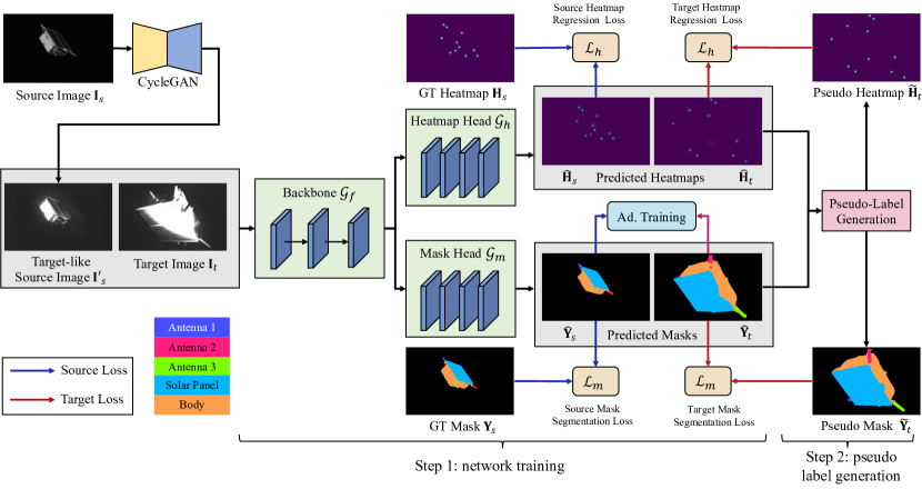
Figure 2: Overview of our self-training framework. The satellite is represented as a set of sparse keypoints and dense fine-grained masks. The source image $\mathbf{I}_{s}$ is first transformed into a target-like source image $\mathbf{I}^{\prime}_{s}$ using a well-trained CycleGAN [48]. The neural network consists of a backbone $\mathcal{G}_{f}$, a heatmap head $\mathcal{G}_{h}$, and a mask head $\mathcal{G}_{m}$. The optimization comprises two iterative steps. In the first step, pseudo mask $\tilde{\mathbf{Y}}_{t}$ and pseudo heatmap $\tilde{\mathbf{H}}_{t}$ are fixed, and the network $\mathcal{G}_{f,h,g}$ are trained using multi-task losses. In the second step, the parameters of the neural network are fixed, and the predicted mask $\hat{\mathbf{Y}}_{t}$ and heatmap $\hat{\mathbf{H}}_{t}$ are used to generate pseudo labels. (Best viewed in color.)

III-D Extended Framework with Multi-task Learning

To tackle the above problem, we note that the fine-grained masks in Fig. 1 provide rich dense descriptions with domain-agnostic structural context. Therefore, we apply segmentation as an auxiliary task of heatmap regression to improve pose estimation performance. In the following paragraphs, we first perform output-level alignment [19] using adversarial training, and then extend the minimization problem in Eq. (7) with the auxiliary task.

As shown in Fig. 2, we extend the basic network with a mask head $\mathcal{G}_{m}$ to predict the fine-grained mask $\hat{\mathbf{Y}}=\mathcal{G}_{m}(\mathcal{G}_{f}(\mathbf{I}))$ for each image. These masks contain domain-agnostic information, which can be used to align the source and target samples by adversarial training. Hence, we build a discriminator $\mathcal{G}_{d}$ to predict the domain label of each sample. The discriminator $\mathcal{G}_{d}$ receives the detached mask predictions from both domains and is trained using the BCE loss,

$$\mathcal{L}_{d}(\hat{\mathbf{Y}}_{t},\hat{\mathbf{Y}}_{s})=-\frac{1}{HW}\sum_{i=1}^{H}\sum_{j=1}^{W} \log(\mathcal{G}_{d}(\hat{\mathbf{Y}}_{s})(i,j,1))+$$

$$\log(\mathcal{G}_{d}(\hat{\mathbf{Y}}_{t})(i,j,0))$$ (10)

where $\hat{\mathbf{Y}}_{s}$ and $\hat{\mathbf{Y}}_{t}$ are the predicted masks of the source and target samples, respectively. To bridge the domain gap, we expect the mask predicted by the network $\mathcal{G}_{f,m}$ to fool the discriminator. Therefore, we perform an adversarial loss on the predicted masks of the target images and backpropagate the gradient.

$$\mathcal{L}_{adv}(\hat{\mathbf{Y}}_{t})=-\frac{1}{HW}\sum_{i=1}^{H}\sum_{j=1}^{W}\log(\mathcal{G}_{d}(\hat{\mathbf{Y}}_{t})(i,j,1))$$ (11)

Furthermore, we introduce a rendering function $\mathcal{R}$ to enhance the geometrical constraints. Given the pose $[\mathbf{R}|\bm{t}]$, the mask $\mathbf{Y}$ can be obtained through the rendering function,

$$\mathbf{Y}=\mathcal{R}(\mathbf{R},\bm{t},\mathcal{M},\mathbf{K})$$ (12)

Similar to the projection function $\mathcal{F}$, the rendering function $\mathcal{R}$ also provides the same geometrical constraints on source and target samples. This is because the 3D mesh of the satellite and the camera parameters are the same in different domains. For source samples, the network $\mathcal{G}_{f,m}$ is supervised using the ground-truth masks. For unlabeled target images, the pseudo masks are obtained by sending the latent variables in Eq. (7), i.e., the target poses, to the rendering function $\mathcal{R}$. Therefore, the minimization problem depicted in Eq. (7) is extended with the tasks of segmentation and adversarial training,

$$\begin{array}[]{*3{>{\displaystyle}l}p{0.1cm}}&\min_{\mathcal{G}_{f,h,m},\mathcal{T}_{t}}\max_{\mathcal{G}_{d}}\frac{1}{N_{s}}\sum_{i=1}^{N_{s}}\left[\mathcal{L}_{h}(\hat{\mathbf{H}}_{s}^{i},\mathbf{H}_{s}^{i})+\lambda_{m}\mathcal{L}_{m}(\hat{\mathbf{Y}}_{s}^{i},\mathbf{Y}_{s}^{i})\right]+\\ &\frac{1}{N_{t}}\sum_{j=1}^{N_{t}}\left[\mathcal{L}_{h}(\hat{\mathbf{H}}_{t}^{j},\tilde{\mathbf{H}}_{t}^{j})+\lambda_{m}\mathcal{L}_{m}(\hat{\mathbf{Y}}_{t}^{j},\tilde{\mathbf{Y}}_{t}^{j})+\lambda_{a}\mathcal{L}_{adv}({\hat{\mathbf{Y}}_{t}^{j}})\right]\\ \end{array}$$ (15)

$$\begin{array}[]{r@{\;}l}\operatorname{s.t.}&\tilde{\mathbf{H}}_{t}^{j}=\mathcal{F}(\mathbf{R}_{t}^{j},\bm{t}_{t}^{j},\mathcal{P},\mathbf{K}),\;\tilde{\mathbf{Y}}_{t}^{j}=\mathcal{R}(\mathbf{R}_{t}^{j},\bm{t}_{t}^{j},\mathcal{M},\mathbf{K}),\\ &\mathcal{T}_{t}^{i}=[\mathbf{R}_{t}^{j}|\bm{t}_{t}^{j}]\in\mathbb{SE}_{3}\cup\{\mathbf{0}\}\vspace{1ex},\;j=1,2,\dots,N_{t}\\ \end{array}$$

where $\lambda_{m}$ and $\lambda_{a}$ are the weights for the mask loss and the adversarial loss, respectively. $\mathcal{L}_{m}$ is the cross-entropy loss for segmentation. We refer to $\tilde{\mathbf{Y}}$ as the pseudo mask. Again, by optimizing the loss in Eq. (15), the network $\mathcal{G}_{f,h,m}$ should perform well on the target domain, while the pseudo labels, including pseudo heatmaps, masks, and poses, should approximate the ground truth.

III-E Iterative Optimization and Pseudo Label Generation

We observe that the variables in Eq. (15) can be divided into two classes: the network parameters and the poses of target samples. Following [23], we adopt iterative procedures to optimize Eq. (15):

1. Fix the pseudo labels (or initialize $\mathcal{T}_{t}$ as $\{\mathbf{0}\}$) and train the network $\mathcal{G}_{f,h,m,d}$;

2. Fix the network, optimize poses $\mathcal{T}_{t}$, and generate pseudo labels.

We take the combination of these two steps as one round and take several rounds to optimize Eq. (15).

In the first step, when the pseudo heatmaps and pseudo masks are fixed, the minimization problem in Eq. (7) is simplified as,

$$\begin{array}[]{*3{>{\displaystyle}l}p{0.1cm}}&\min_{\mathcal{G}_{f,h,m}}\max_{\mathcal{G}_{d}}\frac{1}{N_{s}}\sum_{i=1}^{N_{s}}\left[\mathcal{L}_{h}(\hat{\mathbf{H}}_{s}^{i},\mathbf{H}_{s}^{i})+\lambda_{m}\mathcal{L}_{m}(\hat{\mathbf{Y}}_{s}^{i},\mathbf{Y}_{s}^{i})\right]+\\ &\frac{1}{N_{t}}\sum_{j=1}^{N_{t}}\left[\mathcal{L}_{h}(\hat{\mathbf{H}}_{t}^{j},\tilde{\mathbf{H}}_{t}^{j})+\lambda_{m}\mathcal{L}_{m}(\hat{\mathbf{Y}}_{t}^{j},\tilde{\mathbf{Y}}_{t}^{j})+\lambda_{a}\mathcal{L}_{adv}({\hat{\mathbf{Y}}_{t}^{j}})\right]\end{array}$$ (16)

It is equal to train the neural network using the labeled source samples and the pseudo-labeled target samples. In the second step, when the network parameters are fixed, the minimization problem in Eq. (15) is simplified as,

$$\min_{\mathcal{T}_{t}}\frac{1}{N_{t}}\sum_{j=1}^{N_{t}}\left[\mathcal{L}_{h}(\hat{\mathbf{H}}_{t}^{j},\tilde{\mathbf{H}}_{t}^{j})+\lambda_{m}\mathcal{L}_{m}(\hat{\mathbf{Y}}_{t}^{j},\tilde{\mathbf{Y}}_{t}^{j})\right]$$ (17)

$$\begin{array}[]{r@{\;}l}\operatorname{s.t.}&\tilde{\mathbf{H}}_{t}^{j}=\mathcal{F}(\mathbf{R}_{t}^{j},\bm{t}_{t}^{j},\mathcal{P},\mathbf{K}),\;\tilde{\mathbf{Y}}_{t}^{j}=\mathcal{R}(\mathbf{R}_{t}^{j},\bm{t}_{t}^{j},\mathcal{M},\mathbf{K}),\\ &\mathcal{T}_{t}^{i}=[\mathbf{R}_{t}^{j}|\bm{t}_{t}^{j}]\in\mathbb{SE}_{3}\cup\{\mathbf{0}\}\vspace{1ex},\;j=1,2,\dots,N_{t}\\ \end{array}$$

It is equal to optimize the target poses to minimize the loss, by simultaneously aligning the heatmaps and masks generated using functions $\mathcal{F}$ and $\mathcal{R}$ with the ones predicted by the network. However, for the classification loss $\mathcal{L}_{m}$, there is a trivial solution by ignoring all pseudo heatmaps, i.e., $\mathcal{T}_{s}=\{\mathbf{0}\}$. Therefore, we leverage the predicted heatmaps to estimate poses and then generate pseudo labels.

Specifically, we decode the predicted heatmap $\hat{\mathbf{H}}_{t}$ of the target image into the 2D coordinates of keypoints, which are then used to generate putative correspondences $\{(\hat{\bm{p}}_{t}^{k},\bm{P}^{k})\}_{k=1}^{N_{p}}$. Next, the estimated pose $[\hat{\mathbf{R}}|\hat{\bm{t}}]$ and the number of inliers $N_{in}$ can be obtained by solving Eq. (5). We kindly refer to the readers to our previous work [15] for the detail solution to Eq. (5). Furthermore, we take $N_{in}$ as the confidence of the estimated pose and select the estimated pose as a pseudo pose if $N_{in}\geq N_{th}$. Otherwise, the pseudo pose is set to 0 and the corresponding sample is excluded during network retraining. A smaller $N_{th}$ encourages more estimated poses to be used to generate pseudo labels for model training. Additionally, for target samples with $N_{in}<N_{th}$, we generate pseudo masks using the approach proposed by [24].

III-F Discussion

Our self-training framework is built upon the geometrical constraints, which are provided by the projection function $\mathcal{F}$ and the rendering function $\mathcal{R}$. We try to provide a mathematical proof of the geometrical constraints in this section from the perspective of probability distribution. Since the functions $\mathcal{F}$ and $\mathcal{R}$ have the same formation, we only present the proof of the function $\mathcal{F}$ in the remainder of this section.

Equation (6) has four input parameters, including satellite pose $[\mathbf{R}|\bm{t}]$, 3D landmarks $\mathcal{P}$, and camera intrinsic matrix $\mathbf{K}$. Since $\mathcal{P}$ and $\mathbf{K}$ are constant, if the poses of the satellite in the source and target domain are equal, the heatmaps in both domains are the same.

$$\begin{split}&[\mathbf{R}_{s}|\bm{t}_{s}]=[\mathbf{R}_{t}|\bm{t}_{t}]\Rightarrow\\ &\mathcal{F}(\mathbf{R}_{s},\bm{t}_{s},\mathcal{P},\mathbf{K})=\mathcal{F}(\mathbf{R}_{t},\bm{t}_{t},\mathcal{P},\mathbf{K})\Rightarrow\\ &\mathbf{H}_{s}=\mathbf{H}_{t}\end{split}$$ (18)

Therefore, when conditioned on the satellite pose, the heatmap distributions in source and target domains are the same.

$$P(\mathbf{H}_{s}|\mathbf{R}_{s},\bm{t}_{s})=P(\mathbf{H}_{t}|\mathbf{R}_{t},\bm{t}_{t})$$ (19)

On the other hand, the heatmap distributions can be marginalized on the satellite poses as following,

$$\begin{split}P(\mathbf{H}_{s})&=\int\int P(\mathbf{H}_{s}|\mathbf{R}_{s},\bm{t}_{s})P(\mathbf{R}_{s}=\mathbf{R},\bm{t}_{s}=\bm{t})\;\mathrm{d}\mathbf{R}\mathrm{d}\bm{t}\\ P(\mathbf{H}_{t})&=\int\int P(\mathbf{H}_{t}|\mathbf{R}_{t},\bm{t}_{t})P(\mathbf{R}_{t}=\mathbf{R},\bm{t}_{t}=\bm{t})\;\mathrm{d}\mathbf{R}\mathrm{d}\bm{t}\\ \end{split}$$ (20)

By combining Eq. (1), Eq. (19), and Eq. (20), we can get the conclusion that the heatmaps in the source and target domain have the same distribution, i.e.,

$$P(\mathbf{H}_{s})=P(\mathbf{H}_{t})$$ (21)

Therefore, the geometrical constraint provided by the projection function $\mathcal{F}$ is domain-agnostic.

What’more, the similar conclusion also holds for the rendering function $\mathcal{R}$, i.e., $P(\mathbf{Y}_{s})=P(\mathbf{Y}_{t})$. The fine-grained mask provides dense representation, while the keypoints heatmap is sparse and leads to significant information loss. Hence, we perform output level adaptation to match mask distributions between source and target domain in Sec. III-D.

IV EXPERIMENTAL RESULTS

We present experimental details and results in this section. We first introduce the dataset and the metrics used in the experiments in Sec. IV-A. Then, Sec. IV-B presents the details of implementation. Next, the key components of the proposed approach are studied in Sec. IV-C. We compare our approach with the state-of-the-art methods in Sec. IV-D. Finally, Sec. IV-E presents the runtime analysis.

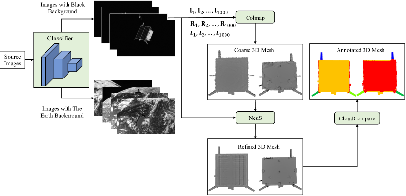
Figure 3: Pipeline of 3D mesh reconstruction and annotation.

IV-A Dataset and Metrics

Dataset. We conduct experiments on the SPEED+ [22] dataset to demonstrate the effectiveness of our method. The SPEED+ [22] dataset comprises images of the Tango spacecraft from the PRISMA [49] mission, consisting of three distinct domains, i.e., synthetic, lightbox, and sunlamp. Each image has a resolution of $1920\times 1200$ and contains a single object. The synthetic domain comprises 59,960 images labeled with poses, which are generated using an OpenGL-based stimulator. The lightbox and sunlamp domains contain 6,740 and 2,791 images of a model of the same spacecraft captured in a robotic simulation environment. The satellite in the lightbox domain is illuminated by several lightboxes to approximate the diffuse light of Earth, while the same object in the sunlamp domain is exposed to an arc lamp to simulate the direct sunlight. Since the annotations for lightbox and sunlamp domains are not released, there are two UDA tasks with respect to SPEED+, including synthetic$\to$lightbox and synthetic$\to$sunlamp.

Metrics. We adopt the metrics used in SPEC2021. The rotation error is defined as the angle between the predicted quaternion $\hat{\bm{q}}$ and the ground truth $\bm{q}$, i.e., $E_{q}=2\arccos(\hat{\bm{q}}^{T}\bm{q})$. The translation error is defined as the difference between the predicted value $\hat{\bm{t}}$ and the ground truth $\bm{t}$, i.e., $E_{t}=\|\hat{\bm{t}}-\bm{t}\|_{2}$. Given an image, the scores for rotation and translation are defined as ${S}_{q}=E_{q}$ and ${S}_{t}=E_{t}/\|\bm{t}\|_{2}$, respectively. The overall score is given as

$$S=\begin{cases}0,&\text{if}\quad{S}_{q}<\theta_{q}\;\text{and}\;{S}_{t}<\theta_{t}\\ {S}_{q}+{S}_{t},&\text{otherwise}\end{cases}$$ (22)

where $\theta_{q}=0.169^{\circ}$ and $\theta_{t}=2.173\times 10^{-3}$ are the thresholds, which are determined by the calibration results of the facility used to create the dataset [22].

IV-B Implementation Details

Mesh reconstruction and data preparation. Since the 3D mesh of the satellite is not provided in SPEED+, we reconstruct the 3D mesh $\mathcal{M}$ and 3D landmarks $\mathcal{P}$ using source samples. However, due to illumination variations and material discrepancies, the texture of satellite is not domain-agnostic, while the geometrical model are the same for the source and target samples. Therefore, we reconstruct the texture-less 3D mesh of the satellite to leverage the geometrical constraints.

The pipeline for 3D mesh reconstruction and annotation is shown in Fig. 3. Note that, the source images can have two types of background: the earth background and the black background. Since the earth background usually introduces noise during reconstruction, we first train a classifier to select images with a black background. Next, to tackle the scale issue, we select 1000 images using the criterion of 4.5m $\leq\|\bm{t}\|_{2}\leq$ 5m, where $\bm{t}$ is the translation of the satellite to the camera. We first reconstruct the coarse mesh using the Multi-View Stereo (MVS) approach provided by colmap [50, 51]. Next, we use the Neural Implicit Surfaces (NeuS) [52] approach to refine the mesh. The refined mesh is then annotated with 5 categories, including antenna 1-3, solar panel, and body. Meanwhile, we select 11 landmarks on the surface of the mesh, following previous works [12, 15]. Finally, given the ground-truth poses for source images and the pseudo poses for target images, we use Blender to render the mesh for fine-grained masks, and use the pinhole camera model [53] to obtain 2D keypoints.

Architecture details. Our network comprises four modules: a backbone, a mask head, a heatmap head, and a discriminator. We construct the backbone using a transformer-based HRNet network [54], i.e., HRFormer-S with 7.8M parameters. The backbone extracts feature maps at $\frac{1}{4}$ resolution of the input images. The output channel number is 32. The heatmap head and the mask head are constructed using an atrous-spatial-pyramid-pooling (ASPP) module [55], respectively. The module consists of five parallel branches: a global average pooling layer, a 1 $\times$ 1 convolution layer, and three 3 $\times$ 3 atrous convolution layers with rates of (6, 12, 18). Then, all feature maps are concatenated into one feature, whose channel number is adjusted using a 1 $\times$ 1 convolution layer. The discriminator has $4\times 4$ convolutional layers with channel numbers (16, 32, 64, 128, 1). The first and the second layers have a stride of 1 while others have a stride of 2. Each convolutional layer except the last one is followed by a leaky ReLU parameterized by 0.2.

Experimental details. We implement the network using the PyTorch library and train our model using the AdamW [56] optimizer. All images are resized to the resolution of $640\times 400$. The source images are first translated into target-like images using a CycleGAN [48] to reduce the bias towards the source domain. During training, we apply different data augmentation strategies on source and target samples using Albumentations [57] with the default parameter setting. The data augmentation on target samples composes of random horizontal and vertical flipping, random translating, scaling, and rotating. On source samples, the additional augmentation includes random gaussian noise and random blur. We adopt a multi-level learning strategy to enhance domain adaptation by applying the prediction heads after stages 3 and 4 of the backbone. The balance parameters of the losses in stages 3 and 4 are set to 0.1 and 1, respectively. During pseudo-label generation, threshold $N_{th}$ is empirically set to 8.

IV-C Ablation Study

We conduct a series of ablation experiments to investigate the critical components of our approach, including self-training, adversarial training, mask prediction, and pseudo-label generation with the geometrical constraints. Due to the unavailability of pose labels of target samples, we manually annotate 100/50 images from the lightbox/sunlamp domain by selecting semantic keypoints and solving the PnP problem. We adopt the manually annotated samples as the validation set. For each setting, we take 3 rounds to optimize Eq. (15) and define the first round as the pretraining stage. During pretraining, we set the initial learning rate to 0.001 and train the network for 12 epochs with a batch size of 5. For the second and the third rounds, we decrease the learning rate to 0.0005 and optimize the network for 10 epochs, which contains 10, 000 steps. The results are reported in Table I. The neural network trained after round $j$ under the $i$th setting is denoted by $\mathcal{G}_{i}^{j}$. Especially, model $\mathcal{G}^{0}_{1}$ is the trivial baseline, as it is trained on target-like images transformed using a CycleGAN and no other UDA method is used.

TABLE I: Ablation Study of the key components on the SPEED+ dataset.

Model	w/o	w/o	part	round	lightbox			sunlamp
	adv.1	con.2	num		$E_{t}$ [m]	$E_{q}$ [∘]	$S$ [-]	$E_{t}$ [m]	$E_{r}$ [∘]	$S$ [-]
$\mathcal{G}_{1}$		$\surd$	0	0	1.0069	36.0853	0.7952	0.9986	39.3665	0.8651
				1	0.8524	21.7186	0.5180	0.9242	30.2367	0.6861
				2	0.9339	24.4870	0.5691	0.9738	29.0898	0.6846
$\mathcal{G}_{2}$	$\surd$	$\surd$	0	0	0.2793	20.6284	0.4251	0.5211	32.1571	0.6576
				1	0.2454	15.1444	0.3136	0.2214	16.4786	0.3324
				2	0.2307	10.8686	0.2315	0.1536	11.2180	0.2226
$\mathcal{G}_{3}$	$\surd$	$\surd$	1	0	0.3662	20.4000	0.4175	0.4850	21.0174	0.4390
				1	0.2928	14.6781	0.3033	0.2820	14.6238	0.3011
				2	0.3767	11.1182	0.2523	0.1669	11.9669	0.2359
$\mathcal{G}_{4}$	$\surd$		5	0	0.3235	16.6921	0.2865	0.2043	8.9460	0.1873
				1	0.2342	11.1159	0.2386	0.1310	6.3235	0.1310
				2	0.2310	11.7523	0.2463	0.1104	5.2222	0.1103
$\mathcal{G}_{5}$	$\surd$	$\surd$	5	0	0.3235	16.6921	0.2865	0.2043	8.9460	0.1873
				1	0.2346	10.8023	0.2302	0.1068	5.2535	0.1108
				2	0.2039	10.5052	0.2205	0.0963	4.6960	0.0988

• with/without adversarial training;

• with/without domain-agnostic geometrical constraints.

Self-training. In each setting, models $\mathcal{G}^{1}$ and $\mathcal{G}^{2}$ achieve smaller pose estimation errors than model $\mathcal{G}^{0}$. This demonstrates that the self-training framework can promote model performance for the UDA task in satellite pose estimation.

Adversarial training. We construct a baseline $\mathcal{G}_{1}$ within the basic framework by optimizing Eq. (7). Then, we extend the framework with adversarial training, by aligning the features extracted by the backbone. The model trained in the extended framework is denoted by $\mathcal{G}_{2}$. For each round, model $\mathcal{G}_{2}^{i}$ significantly outperforms the baseline $\mathcal{G}_{1}^{i}$, $i=0,1,2$. After the pretraining stage, model $\mathcal{G}_{2}^{0}$ reduce the translation error from 1.0069m/0.9986m to 0.2793m/0.5211m for the lightbox/sunlamp domain. When round = 2, model $\mathcal{G}_{2}^{2}$ reduces the scores by half for both domains. These results demonstrate the effectiveness of adversarial training.

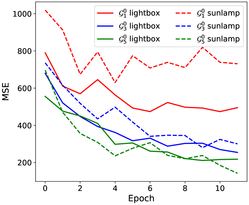
Figure 4: The mean square errors (MSE) between the predicted and ground-truth keypoints in the pretraining stage.

Mask prediction. We further extend the baseline with multi-task learning by appending a mask head after the backbone. The mask head predicts a binary mask (in model $\mathcal{G}_{3}$) or a fine-grained mask (in model $\mathcal{G}_{5}$) of the satellite. Different from model $\mathcal{G}_{2}$, we apply adversarial training by aligning the predictions of the mask head. Model $\mathcal{G}_{3}$ achieves more accurate pose estimation results than model $\mathcal{G}_{2}$ in all rounds except the last one in terms of total score $S$. Another experimental evidence is provided by the comparison between model $\mathcal{G}_{3}$ and model $\mathcal{G}_{5}$. When round = 0, model $\mathcal{G}_{5}^{0}$ significantly reduces the estimation error by nearly 30% and 50% in terms of score $S$ for both domains. The key reason is that the mask head in model $\mathcal{G}_{5}$ provides more fine-grained predictions and thus effectively enhances structural constraints and contextual information. Moreover, using the proposed self-training framework, model $\mathcal{G}_{5}^{2}$ achieves the best pose estimation results in all metrics and on all tasks. Therefore, leveraging fine-grained segmentation as an auxiliary task has positive impacts on 2D keypoints regression, resulting in better performance of satellite pose estimate across domains.

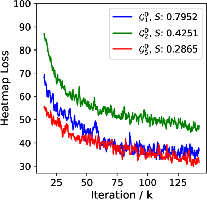
(a) lightbox

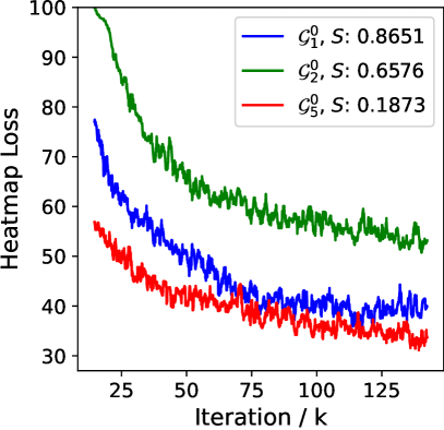
(b) sunlamp

Figure 5: Comparisons of the training curves of model $\mathcal{G}_{0}^{0}$, $\mathcal{G}_{2}^{0}$, and $\mathcal{G}_{5}^{0}$.

To better analyze the function of the fine-grained segmentation, we compare the mean square error (MSE) between the ground-truth and the predicted keypoints on the validation set after each epoch. Specifically, we report the MSEs of the pretrained models, including $\mathcal{G}_{1}^{0}$, $\mathcal{G}_{3}^{0}$, and $\mathcal{G}_{5}^{0}$, and the results are shown in Fig. 4. Note that, model $\mathcal{G}_{1}^{0}$ always achieves the largest MSEs on lightbox and sunlamp domains, while $\mathcal{G}_{3}^{0}$ benefits from the binary segmentation task. Moreover, $\mathcal{G}_{5}^{0}$ shows the highest accuracy by predicting the fine-grained masks. It illustrates that the fine-grained segmentation can effectively improve the domain adaptation performance, and thus prevent the optimization of Eq. (15) converging at local optima.

(a) lightbox

(b) sunlamp

Figure 6: Visualization of pseudo labels of target samples. The first column shows the pseudo keypoints generated without and with the geometrical constraints in green crosses and blue points, respectively. The red vectors illustrate the differences between the two types of pseudo keypoints. The second/last column shows pseudo masks generated without/with the geometrical constraints.

(a) lightbox

(b) sunlamp

Figure 7: Visualization of pose estimation on target samples. The results achieved with and without our framework are shown in green and red colors, respectively.

Geometrical constraints. We also study the role of the geometrical constraints, which are used during pseudo-label generation. We directly generate pseudo heatmaps and pseudo masks according to model predictions. The model trained using this setting is denoted by $\mathcal{G}_{4}$. In terms of three metrics on both domains, models $\mathcal{G}_{4}^{1}$ and $\mathcal{G}_{4}^{2}$ show degraded performance compared to $\mathcal{G}_{5}^{1}$ and $\mathcal{G}_{5}^{2}$, respectively. The performance degradation can be ascribed to the annotation noise in pseudo labels. With the geometrical constraints, models $\mathcal{G}_{5}^{1}$ and $\mathcal{G}_{5}^{2}$ are trained using more clean and more accurate pseudo labels and thus show superior performance. The visual comparison between pseudo labels generated with and without geometrical constraints is illustrated in Fig. 6.

Multi-task learning. We adopt adversarial training and mask segmentation to promote keypoint heatmap regression. In Fig. 5, we study the effectiveness of multi-task learning strategies, by comparing the heatmap losses of model $\mathcal{G}_{0}^{0}$, $\mathcal{G}_{2}^{0}$, and $\mathcal{G}_{5}^{0}$ during training. On each domain, model $\mathcal{G}_{0}^{0}$ overfits more to source samples and generalizes less to target images, because it is only trained using source data. Model $\mathcal{G}_{2}^{0}$ performs feature level adaptation using adversarial training. Although model $\mathcal{G}_{2}^{0}$ has larger heatmap losses, it achieves better pose estimation accuracy than model $\mathcal{G}_{0}^{0}$. In contrast, $\mathcal{G}_{5}^{0}$ performs output level adaptation by introducing fine-grained segmentation, resulting in the smallest losses and the best pose estimation accuracy on each domain. The reason is that the feature level adaptation is performed in the high-dimensional space, leading to the alignment of easier patterns [19]. Consequently, the feature distributions cannot be effectively matched. This demonstrates the effectiveness of our multi-task learning strategies.

IV-D Comparison with the State-of-the-Art Methods

We take KRN [13] and SPNv2 [58] as the baseline methods. SPNv2 [58] is based on EfficientDet [59] and comprises three prediction heads: the EfficientPose head [60] for object presence, bounding box, target rotation and translation; the heatmap head for the 2D heatmaps; the segmentation head for the binary mask of the satellite. Other technologies employed by SPNv2 include multi-scale design [59, 60], extensive data augmentation [61], style augmentation [62], AdaBN [63], and entropy minimization. Different from these methods, we utilize the geometrical constraints to develop a self-training framework and explore the fine-grained segmentation to boost performance.

To achieve better performance, we add an upsampling layer followed by a $3\times 3$ convolution after the backbone and thus increase the feature resolution by a scaling factor 2. We take multiple rounds to optimize Eq. (15) and then compare our method with KRN [13], SPNv2 [58], and top-performing methods in SPEC2021. The results are listed in Table II. On the sunlamp domain, our approach outperforms all other methods in terms of translation and rotation scores, taking the 1st place in the challenge. More importantly, our method surpasses KRN [13] trained using real annotations by more than half in terms of score $S$. On the lightbox domain, our approach shows competitive performance and has won the 3rd place in the challenge. Figure 7 visualizes results estimated by the models trained with and without the proposed framework. Note that, our model can handle intense imaging noise, complicated illuminations, surface reflection, and pose variations.

TABLE II: Comparison with the state-of-the-art methods and the top-performing methods in SPEC2021.

Methods/Team	lightbox			sunlamp
	$S_{t}$	$S_{q}$	$S$	$S_{t}$	$S_{q}$	$S$
KRN [13]	-	-	1.12	-	-	3.73
+ Style aug. [62] 1	-	-	0.81	-	-	1.32
+ Oracle 2	-	-	0.15	-	-	0.13
SPNv2 [58]	-	-	0.122	-	-	0.198
UT Austin Seeker RD	0.3626	0.1532	0.5158	0.3589	0.1227	0.4816
bbnc	0.0940	0.4344	0.5284	0.0794	0.3832	0.4626
chusunhao	0.0303	0.2859	0.3162	0.0573	0.7567	0.8140
u3s_lab	0.0530	0.1692	0.2221	0.0297	0.1089	0.1386
haoranhuang_njust	0.0279	0.1419	0.1698	0.0248	0.1467	0.1715
VPU	0.0178	0.0799	0.0977	0.0072	0.0493	0.0565
TangoUnchained	0.0139	0.0556	0.0695	0.0109	0.0750	0.0859
lava1302 (ours)	0.0464	0.1163	0.1627	0.0069	0.0476	0.0545

• trained with style augmentation;

• trained with the ground-truth poses of target samples.

TABLE III: Run-time analysis with different backbones and feature resolutions.

Backbone	Feat.	Param.	Mem.	Time	lightbox			sunlamp
	Stride	[M]	[G]	[ms]	$E_{\textrm{t}}$ [m]	$E_{\textrm{r}}$ [rad]	$S_{\textrm{pose}}$ [-]	$E_{\textrm{t}}$ [m]	$E_{\textrm{r}}$ [rad]	$S_{\textrm{pose}}$ [-]
HRNet-W32 [64]	4	28.01	1.69	36.0	0.218	12.259	0.253	0.119	8.259	0.163
HRFormer-S [54]	4	8.19	1.53	57.1	0.204	10.505	0.221	0.096	4.696	0.099
HRFormer-S [54]	2	8.21	1.84	57.3	0.138	3.223	0.078	0.042	1.616	0.036

IV-E Runtime Performance

We follow the experimental settings in ablation study and compare the runtime performance of the models using different backbones and feature map resolutions. The experiments are conducted on a PC with an Nvidia GTX 3090 GPU. Table III reports the results. We first replace the transformer-based backbone with a CNN-based backbone, i.e., HRNet [64]. Although the running time is shorter at the expense of larger parameter sizes and memory consumption, the pose estimation performance drops from 0.221/0.099 to 0.253/0.163 on lightbox/sunlamp in terms of score $S$. Furthermore, we add an upsampling layer followed by a $3\times 3$ convolution after the backbone, to increase the feature resolution by a scaling factor 2. We observe significant improvements of pose estimation at the expense of increased computation. However, the increase in running time is only about 0.35% (which is negligible) since the upsampling module and the prediction heads are very simple.

V LIMITATION AND CONCLUSION

V-A Limitation

One apparent limitation of our method is that only the predicted heatmaps are used to generate pseudo poses in Sec. III-E, while the predicted masks are ignored. Another limitation would be the sparse representation of the satellite using a set of keypoints. Note that the pose estimation could be less stable when these keypoints are invisible due to truncation, low light, or high reflection. The third limitation of this work is that the implementations of the projection function $\mathcal{F}$ and the rendering function $\mathcal{R}$ are non-differentiable and performed offline. Future work is needed, specifically in incorporating a differentiable rendering engine to simultaneously achieve online self-training and pose refinement based on fine-grained masks.

V-B Conclusion

This paper explores the domain-agnostic geometrical constraints to achieve unsupervised domain adaptation in satellite pose estimation. The task is formulated as a minimization problem in a self-training framework by taking the target poses as latent variables. Meanwhile, the fine-grained segmentation is introduced as an auxiliary task to improve performance. The experimental results demonstrate that our method achieves superior performance.

Zi Wang received the B.E. degree in measuring and controlling technologies and instruments from Tianjin University (TJU), Tianjin, China, in 2016, and the M.E. degree in Aeronautical and Astronautical Science and Technology from National University of Defense Technology (NUDT), Changsha, China, in 2018. He was a visiting Ph.D. student in Sun Yat-sen University from 2021 to 2022. He is currently pursuing the Ph.D. degree with the College of Aerospace Science and Engineering, NUDT. His current research interests include transfer learning and object pose estimation.

Minglin Chen is currently a Ph.D. student at Sun Yat-Sen University (SYSU). He received his M.Eng. degree in software engineering at the University of Chinese Academy of Science (UCAS) in 2020, and his B.Eng. degree in communication engineering at South China Normal University (SCNU) in 2017. His research interests lie in the intersection of computer vision and computer graphics.

Yulan Guo received the B.Eng. and Ph.D. degrees from National University of Defense Technology (NUDT) in 2008 and 2015, respectively. He has authored over 100 articles in journals and conferences. His current research interests focus on 3D vision, particularly on 3D feature learning, 3D modeling, 3D object recognition, and scene understanding. He serves as an associate editor for IEEE Transactions on Image Processing, IET Computer Vision, IET Image Processing, and Computers & Graphics. He also served as a guest editor for IEEE Transactions on Pattern Analysis and Machine Intelligence, and an area chair for CVPR 2023/2021, ICCV 2021, and ACM Multimedia 2021.

Zhang Li received the Ph.D. degree in biomedical engineering from the Delft University of Technology, Delft, The Netherlands, in 2015. He is an Associate Professor with the College of Aerospace Science and Engineering, National University of Defense Technology, Changsha, China. He authored over 20 papers in high-ranking journals and conferences, such as IEEE TRANSACTIONS ON MEDICAL IMAGING and IEEE TRANSACTIONS ON BIOMEDICAL ENGINEERING. His research interests include biomedical image analysis and particularly image registration.

Qifeng Yu received the B.S. degree from Northwestern Polytechnic University, Xi’an, China, in 1981, the M.S. degree from the National University of Defense Technology, Changsha, China, in 1984, and the Ph.D. degree from Bremen University, Bremen, Germany, in 1996. He is a Professor with the National University of Defense Technology. He has authored three books and published over 100 articles. His main research fields include image measurement, vision navigation, and close-range photogrammetry. Dr. Yu is a member of the Chinese Academy of Sciences.

References

- [1] J. L. Forshaw, G. S. Aglietti, N. Navarathinam, H. Kadhem, T. Salmon, A. Pisseloup, É. Joffre, T. Chabot, I. D. Retat, R. Axthelm, S. Barraclough, A. Ratcliffe, C. Bernal, F. Chaumette, A. Pollini, and W. H. Steyn, “RemoveDEBRIS: An in-orbit active debris removal demonstration mission,” Acta Astronautica, vol. 127, pp. 448–463, 2016.
- [2] A. Flores-Abad, O. Ma, K. D. Pham, and S. Ulrich, “A review of space robotics technologies for on-orbit servicing,” Progress in Aerospace Sciences, vol. 68, pp. 1–26, 2014.
- [3] D. Malyh, S. Vaulin, V. Fedorov, R. Peshkov, and M. Shalashov, “A brief review on in-orbit refueling projects and critical techniques,” Aerospace Systems, vol. 5, pp. 185–196, 2022.
- [4] R. Opromolla and A. Nocerino, “Uncooperative spacecraft relative navigation with lidar-based unscented kalman filter,” IEEE Access, vol. 7, pp. 180 012–180 026, 2019.
- [5] R. Opromolla, G. Fasano, G. Rufino, and M. Grassi, “A model-based 3d template matching technique for pose acquisition of an uncooperative space object,” Sensors (Basel, Switzerland), vol. 15, pp. 6360 – 6382, 2015.
- [6] B. J. Naasz, R. Burns, S. Z. Queen, J. V. Eepoel, J. Hannah, and E. Skelton, “The hst sm4 relative navigation sensor system: Overview and preliminary testing results from the flight robotics lab,” The Journal of the Astronautical Sciences, vol. 57, pp. 457–483, 2009.
- [7] C. Liu and W. Hu, “Relative pose estimation for cylinder-shaped spacecrafts using single image,” IEEE Transactions on Aerospace and Electronic Systems, vol. 50, pp. 3036–3056, 2014.
- [8] C. Meng, Z. Li, H. Sun, D. Yuan, X. Bai, and F. Zhou, “Satellite pose estimation via single perspective circle and line,” IEEE Transactions on Aerospace and Electronic Systems, vol. 54, pp. 3084–3095, 2018.
- [9] X. Zhang, Z. Jiang, H. Zhang, and Q. Wei, “Vision-based pose estimation for textureless space objects by contour points matching,” IEEE Transactions on Aerospace and Electronic Systems, vol. 54, pp. 2342–2355, 2018.
- [10] J. Davis and H. Pernicka, “Proximity operations about and identification of non-cooperative resident space objects using stereo imaging,” Acta Astronautica, vol. 155, pp. 418–425, 2019.
- [11] M. Kisantal, S. Sharma, T. H. Park, D. Izzo, M. Märtens, and S. D’Amico, “Satellite pose estimation challenge: Dataset, competition design, and results,” IEEE Transactions on Aerospace and Electronic Systems, vol. 56, no. 5, pp. 4083–4098, 2020.
- [12] B. Chen, J. Cao, A. Parra, and T.-J. Chin, “Satellite pose estimation with deep landmark regression and nonlinear pose refinement,” in IEEE International Conference on Computer Vision Workshops, 2019, pp. 0–0.
- [13] T. H. Park, S. Sharma, and S. D’Amico, “Towards robust learning-based pose estimation of noncooperative spacecraft,” in AAS/AIAA Astrodynamics Specialist Conference, Portland, Maine, 2019.
- [14] S. Sharma and S. D’Amico, “Neural network-based pose estimation for noncooperative spacecraft rendezvous,” IEEE Transactions on Aerospace and Electronic Systems, vol. 56, pp. 4638–4658, 2020.
- [15] Z. Wang, Z. Zhang, X. Sun, Z. Li, and Q. Yu, “Revisiting monocular satellite pose estimation with transformer,” IEEE Transactions on Aerospace and Electronic Systems, 2022.
- [16] J. Hoffman, E. Tzeng, T. Park, J.-Y. Zhu, P. Isola, K. Saenko, A. Efros, and T. Darrell, “CyCADA: Cycle-consistent adversarial domain adaptation,” in International Conference on Machine Learning, 2018, pp. 1989–1998.
- [17] Y. Ganin, E. Ustinova, H. Ajakan, P. Germain, H. Larochelle, F. Laviolette, M. March, and V. Lempitsky, “Domain-adversarial training of neural networks,” Journal of Machine Learning Research, vol. 17, no. 59, pp. 1–35, 2016.
- [18] Y. Chen, W. Li, C. Sakaridis, D. Dai, and L. V. Gool, “Domain adaptive faster r-cnn for object detection in the wild,” IEEE Conference on Computer Vision and Pattern Recognition, pp. 3339–3348, 2018.
- [19] Y.-H. Tsai, W.-C. Hung, S. Schulter, K. Sohn, M.-H. Yang, and M. Chandraker, “Learning to adapt structured output space for semantic segmentation,” IEEE Conference on Computer Vision and Pattern Recognition, pp. 7472–7481, 2018.
- [20] T.-H. Vu, H. Jain, M. Bucher, M. Cord, and P. Pérez, “ADVENT: Adversarial entropy minimization for domain adaptation in semantic segmentation,” IEEE Conference on Computer Vision and Pattern Recognition, pp. 2512–2521, 2019.
- [21] J. Deng, W. Li, Y. Chen, and L. Duan, “Unbiased mean teacher for cross-domain object detection,” in IEEE Conference on Computer Vision and Pattern Recognition, 2021, pp. 4089–4099.
- [22] T. H. Park, M. Märtens, G. Lecuyer, D. Izzo, and S. D’Amico, “SPEED+: Next-generation dataset for spacecraft pose estimation across domain gap,” in IEEE Aerospace Conference, 2022, pp. 1–15.
- [23] Y. Zou, Z. Yu, B. Kumar, and J. Wang, “Unsupervised domain adaptation for semantic segmentation via class-balanced self-training,” in European Conference on Computer Vision, 2018, pp. 289–305.
- [24] Y. Li, L. Yuan, and N. Vasconcelos, “Bidirectional learning for domain adaptation of semantic segmentation,” in IEEE Conference on Computer Vision and Pattern Recognition, 2019, pp. 6936–6945.
- [25] M. Long, H. Zhu, J. Wang, and M. I. Jordan, “Unsupervised domain adaptation with residual transfer networks,” in Conference on Neural Information Processing Systems, vol. 29, 2016.
- [26] G. Wang, F. Manhardt, X. Liu, X. Ji, and F. Tombari, “Occlusion-aware self-supervised monocular 6D object pose estimation,” IEEE Transactions on Pattern Analysis and Machine Intelligence, vol. PP, 2021.
- [27] X.-S. Gao, X.-R. Hou, J. Tang, and H.-F. Cheng, “Complete solution classification for the perspective-three-point problem,” IEEE Transactions on Pattern Analysis and Machine Intelligence, vol. 25, no. 8, pp. 930–943, 2003.
- [28] T. Grundmann, W. Feiten, and G. von Wichert, “A gaussian measurement model for local interest point based 6 dof pose estimation,” IEEE International Conference on Robotics and Automation, pp. 2085–2090, 2011.
- [29] E. Brachmann, F. Michel, A. Krull, M. Y. Yang, S. Gumhold, and C. Rother, “Uncertainty-driven 6D pose estimation of objects and scenes from a single rgb image,” IEEE Conference on Computer Vision and Pattern Recognition, pp. 3364–3372, 2016.
- [30] B. Tekin, S. N. Sinha, and P. V. Fua, “Real-time seamless single shot 6D object pose prediction,” in IEEE Conference on Computer Vision and Pattern Recognition, 2018, pp. 292–301.
- [31] Y. Hu, J. Hugonot, P. V. Fua, and M. Salzmann, “Segmentation-driven 6D object pose estimation,” in IEEE Conference on Computer Vision and Pattern Recognition, 2019, pp. 3380–3389.
- [32] S. Zakharov, I. Shugurov, and S. Ilic, “DPOD: 6D pose object detector and refiner,” in IEEE Conference on Computer Vision and Pattern Recognition, 2019, pp. 1941–1950.
- [33] Z. Li, G. Wang, and X. Ji, “CDPN: Coordinates-based disentangled pose network for real-time rgb-based 6-dof object pose estimation,” in IEEE Conference on Computer Vision and Pattern Recognition, 2019, pp. 7678–7687.
- [34] T. Hodan, D. Baráth, and J. Matas, “EPOS: Estimating 6D pose of objects with symmetries,” in IEEE Conference on Computer Vision and Pattern Recognition, 2020, pp. 11 700–11 709.
- [35] S. Peng, X. Zhou, Y. Liu, H. Lin, Q. Huang, and H. Bao, “PVNet: Pixel-wise voting network for 6dof object pose estimation,” IEEE Transactions on Pattern Analysis and Machine Intelligence, 2020.
- [36] W. Kehl, F. Manhardt, F. Tombari, S. Ilic, and N. Navab, “SSD-6D: Making rgb-based 3D detection and 6D pose estimation great again,” in IEEE International Conference on Computer Vision, 2017, pp. 1530–1538.
- [37] Y. Hu, P. Fua, W. Wang, and M. Salzmann, “Single-stage 6D object pose estimation,” in IEEE Conference on Computer Vision and Pattern Recognition, 2020, pp. 2927–2936.
- [38] Y. Labb’e, J. Carpentier, M. Aubry, and J. Sivic, “CosyPose: Consistent multi-view multi-object 6D pose estimation,” in European Conference on Computer Vision, 2020.
- [39] G. Wang, F. Manhardt, F. Tombari, and X. Ji, “GDR-Net: Geometry-guided direct regression network for monocular 6D object pose estimation,” in IEEE Conference on Computer Vision and Pattern Recognition, 2021, pp. 16 606–16 616.
- [40] M. Sundermeyer, Z.-C. Marton, M. Durner, and R. Triebel, “Augmented autoencoders: Implicit 3D orientation learning for 6D object detection,” International Journal of Computer Vision, vol. 128, no. 3, pp. 714–729, 2020.
- [41] M. Sundermeyer, M. Durner, E. Y. Puang, Z.-C. Marton, N. Vaskevicius, K. O. Arras, and R. Triebel, “Multi-path learning for object pose estimation across domains,” in IEEE Conference on Computer Vision and Pattern Recognition, 2020, pp. 13 916–13 925.
- [42] Y. Wen, H. Pan, L. Yang, and W. Wang, “Edge enhanced implicit orientation learning with geometric prior for 6D pose estimation,” IEEE Robotics and Automation Letters, vol. 5, pp. 4931–4938, 2020.
- [43] S. Hinterstoisser, V. Lepetit, S. Ilic, S. Holzer, G. Bradski, K. Konolige, and N. Navab, “Model based training, detection and pose estimation of texture-less 3D objects in heavily cluttered scenes,” in Asian Conference on Computer Vision. Springer, 2012, pp. 548–562.
- [44] Y. Xiang, T. Schmidt, V. Narayanan, and D. Fox, “PoseCNN: A convolutional neural network for 6D object pose estimation in cluttered scenes,” Robotics: Science and Systems, 2018.
- [45] Y. Hu, S. Speierer, W. Jakob, P. Fua, and M. Salzmann, “Wide-depth-range 6D object pose estimation in space,” in IEEE Conference on Computer Vision and Pattern Recognition, 2021, pp. 15 870–15 879.
- [46] G. Wilson and D. J. Cook, “A survey of unsupervised deep domain adaptation,” ACM Transactions on Intelligent Systems and Technology, vol. 11, pp. 1 – 46, 2020.
- [47] X. Wang, L. Bo, and F. Li, “Adaptive wing loss for robust face alignment via heatmap regression,” IEEE International Conference on Computer Vision, pp. 6970–6980, 2019.
- [48] J.-Y. Zhu, T. Park, P. Isola, and A. A. Efros, “Unpaired image-to-image translation using cycle-consistent adversarial networks,” in IEEE International Conference on Computer Vision, 2017, pp. 2242–2251.
- [49] S. D’Amico, M. Benn, and J. L. Jørgensen, “Pose estimation of an uncooperative spacecraft from actual space imagery,” International Journal of Space Science and Engineering, vol. 2, no. 2, pp. 171–189, 2014.
- [50] J. L. Schönberger and J.-M. Frahm, “Structure-from-motion revisited,” in IEEE Conference on Computer Vision and Pattern Recognition, 2016.
- [51] J. L. Schönberger, E. Zheng, M. Pollefeys, and J.-M. Frahm, “Pixelwise view selection for unstructured multi-view stereo,” in European Conference on Computer Vision, 2016.
- [52] P. Wang, L. Liu, Y. Liu, C. Theobalt, T. Komura, and W. Wang, “Neus: Learning neural implicit surfaces by volume rendering for multi-view reconstruction,” in Conference on Neural Information Processing Systems, 2021.
- [53] A. Harltey and A. Zisserman, Multiple view geometry in computer vision (2. ed.). Cambridge University Press, 2006.
- [54] Y. Yuan, R. Fu, L. Huang, W. Lin, C. Zhang, X. Chen, and J. Wang, “HRFormer: High-resolution transformer for dense prediction,” in Conference on Neural Information Processing Systems, 2021.
- [55] L.-C. Chen, Y. Zhu, G. Papandreou, F. Schroff, and H. Adam, “Encoder-decoder with atrous separable convolution for semantic image segmentation,” in European Conference on Computer Vision, 2018, pp. 801–818.
- [56] I. Loshchilov and F. Hutter, “Fixing weight decay regularization in adam,” arXiv preprint arXiv:1711.05101, 2017.
- [57] A. Buslaev, V. I. Iglovikov, E. Khvedchenya, A. Parinov, M. Druzhinin, and A. A. Kalinin, “Albumentations: Fast and flexible image augmentations,” Information, vol. 11, no. 2, 2020. [Online]. Available: https://www.mdpi.com/2078-2489/11/2/125
- [58] T. H. Park and S. D’Amico, “Robust multi-task learning and online refinement for spacecraft pose estimation across domain gap,” in 11th International Workshop on Satellite Constellations & Formation Flying, 2022.
- [59] M. Tan, R. Pang, and Q. V. Le, “EfficientDet: Scalable and efficient object detection,” IEEE Conference on Computer Vision and Pattern Recognition, pp. 10 778–10 787, 2020.
- [60] D. Groos, H. Ramampiaro, and E. A. F. Ihlen, “EfficientPose: Scalable single-person pose estimation,” Applied Intelligence, vol. 51, pp. 2518–2533, 2021.
- [61] A. V. Buslaev, A. Parinov, E. Khvedchenya, V. I. Iglovikov, and A. A. Kalinin, “Albumentations: fast and flexible image augmentations,” ArXiv, vol. abs/1809.06839, 2020.
- [62] P. T. G. Jackson, A. Atapour-Abarghouei, S. Bonner, T. Breckon, and B. Obara, “Style augmentation: Data augmentation via style randomization,” in IEEE Conference on Computer Vision and Pattern Recognition Workshops, 2019, pp. 83–92.
- [63] Y. Li, N. Wang, J. Shi, X. Hou, and J. Liu, “Adaptive batch normalization for practical domain adaptation,” Pattern Recognition, vol. 80, pp. 109–117, 2018.
- [64] J. Wang, K. Sun, T. Cheng, B. Jiang, C. Deng, Y. Zhao, D. Liu, Y. Mu, M. Tan, X. Wang, W. Liu, and B. Xiao, “Deep high-resolution representation learning for visual recognition,” IEEE Transactions on Pattern Analysis and Machine Intelligence, vol. 43, pp. 3349–3364, 2021.