Tightening Quadratic Convex Relaxations for the AC Optimal Transmission Switching Problem

Abstract

The Alternating Current Optimal Transmission Switching (ACOTS) problem incorporates line switching decisions into the fundamental AC optimal power flow (ACOPF) problem. The advantages of the ACOTS problem are well-known in terms of reducing the operational cost and improving system reliability. ACOTS optimization models contain discrete variables and nonlinear, non-convex structures, which make it difficult to solve. We derive strengthened quadratic convex (QC) relaxations for ACOTS by combining several methodologies recently developed in the ACOPF literature. First, we relax the ACOTS model with the on/off QC relaxation, which has been empirically observed to be both tight and computationally efficient in approximating the ACOPF problem. Further, we tighten this relaxation by using strong linearization with extreme-point representation, and by adding several types of new valid inequalities. In particular, we derive a novel kind of on/off cycle-based polynomial constraints, by taking advantage of the network structure. Those constraints are linearized using convex-hull representations and implemented in an efficient branch-and-cut framework. We also tighten the relaxation using the optimization-based bound tightening algorithm. Our extensive numerical experiments on medium-scale PGLib instances show that, compared with the state-of-the-art formulations, our strengthening techniques are able to improve the quality of ACOTS relaxations on many of the PGLib instances, with some being substantial improvements.

I Introduction

Transmission switching, with its inception in the 1980s [1], has gained considerable attention in both industry and academia in recent years [2, 3]. The optimal transmission switching (OTS) problem studies how to switch on or off certain transmission lines to modify the network topology in the real-time operation of transmission power grids. Solving the OTS problem brings several benefits that the traditional optimal power flow (OPF) problem solution cannot offer, such as reducing the total operational cost, mitigating transmission congestion, clearing contingencies, and improving engineering limits [4]. Thus, as the modern transmission control and relay technologies evolve, transmission line switching has become an important option in power system operators’ toolkits.

Previous literature on OTS has mainly relied on the DC approximation of the power flow model to avoid the mathematical complexity of the non-convex AC power flow equations. The first formal mathematical model for the OTS problem, proposed in [5], is based on the DC approximation of the power flow equations. In [6], the authors derive a cycle-induced relaxation for a DCOTS model, and characterize the convex hull of this relaxation.

The downside of DCOTS approximation is that the optimal decisions may not necessarily represent accurate power flows or even be infeasible in the AC setting [7]. Those drawbacks motivate the adoption of ACOTS. The ACOTS problem can be formulated as a non-convex mixed-integer nonlinear program (MINLP), which is challenging to solve. Moreover, even in the DC setting, the OTS problem is known to be NP-hard [8]. Several heuristics are proposed for solving the ACOTS problem, e.g., by [9] and [10]. Separately, convex relaxations for ACOTS have gained significant attention in recent years.

The convex relaxations of the ACOTS problem, of which the literature is quite scarce, are built upon the rich literature on ACOPF convex relaxations, such as the second-order cone (SOC) relaxation [11], the quadratic convex (QC) relaxation [12], and the semi-definite programming (SDP) relaxation [13]. For the ACOPF problem, the standard SDP and QC relaxations are at least as strong as the SOC relaxation, while the strength of the SDP and QC relaxations are not comparable. Computationally, the SOC and QC relaxations are faster and more reliable than the SDP relaxation [12]. In the ACOTS setting, [14, 15] propose a QC relaxation that incorporates on/off decision variables, which provides a tight lower bound to the generation-cost minimization objective. We further tighten this on/off version of the QC relaxation with a much stronger linearization and valid inequalities, with some of the latter being novel.

In particular, one type of valid inequalities we incorporate is cycle-based polynomial constraints (“lifted cycle constraints” for short). The lifted cycle constraints were first proposed by [16] as a relaxation to the arc-tangent constraints in ACOPF. Their work provides a reformulated SOC relaxation for ACOPF, strengthened by the McCormick relaxation of the lifted cycle constraints, which is shown to be incomparable to the SDP relaxation. Further, these cycle-based valid inequalities were generalized for the ACOTS problem in [3], which was derived in the rectangular co-ordinates. However, in our work, we develop a new type of lifted cycle constraints based on the QC relaxation of the ACOPF problem, written in polar co-ordinates. Our method takes advantage of the direct access to auxiliary variables representing the trigonometric functions in the QC relaxation. Then we reformulate the on/off version of those lifted cycle constraints for the ACOTS problem, which is new in the literature. In our strengthened formulation, we combine those new constraints and the lifted cycle constraints from [3]. Further, we linearize these polynomial constraints with the tightest extreme-point representation, which captures the convex hull of the lifted cycle constraints for a given cycle.

We further improve the bounds using an optimization-based bound tightening (OBBT) technique. OBBT is often used in MINLPs to tighten relaxation bounds [17]. It has been shown to be an effective bound-tightening method in nonlinear AC power flow models. In [18], the authors use OBBT to tighten an ACOPF-QC relaxation. In [15], the authors use OBBT for an ACOTS-QC relaxation with nonlinear terms linearized using weaker recursive-McCormick relaxations. In our work, we incorporate all the proposed tightening valid inequalities and the ones from the literature within OBBT, to achieve a very tight lower bound for the ACOTS problem.

Our main contributions can be summarized as follows:

(1) We strengthen the ACOTS-QC relaxation with several techniques. First, we linearize the on/off trilinear terms with the tight extreme-point representation. To the best of our knowledge, we are the first to adapt this linearization method to ACOTS. We also reformulate several ACOPF-QC strengthening constraints for the OTS setting, some of which are novel. Compared with the state-of-the-art on/off QC relaxation formulation [19], our strengthened relaxation is shown to provide better lower bounds for many test cases, and some of those improvements are substantial.

(2) We incorporate lifted cycle constraints to further tighten the strengthened ACOTS-QC relaxation. We also derive a novel type of lifted cycle constraint that strengthens the QC relaxations of both ACOPF and ACOTS. We linearize those constraints with the extreme-point representation, which is always tighter than the recursive-McCormick relaxation in the literature. Also, we develop a branch-and-cut framework to efficiently incorporate expensive lifted cycle constraints, which can deal with discrete decisions in the separation process and resulting in significant solution time reductions.

(3) Finally, we use OBBT to further tighten the ACOTS-QC relaxation in conjunction with the branch-and-cut framework for cycle constraints. Combined with other strengthening methods listed in (1) and (2), we obtain the tightest ACOTS relaxation in the literature, to the best of our knowledge.

II Problem Formulations

Nomenclature

II-A Sets and parameters

$\mathcal{N}$

Set of buses (nodes).

$\mathcal{N}^{L}$

Set of leaf buses with no loads.

$\mathcal{N}^{\text{ref}}$

Set of reference buses.

$\cal{G}$

Set of generators.

${\cal{G}}_{i}$

Set of generators at bus $i$.

$\mathcal{A}$

Set of lines (arcs).

$\mathcal{A}^{R}$

Set of arcs in reversed direction.

$\boldsymbol{c}_{0},\boldsymbol{c}_{1},\boldsymbol{c}_{2}$

Generation cost coefficients.

$\mathbf{j}$

Unit imaginary number.

$\boldsymbol{Y}_{ij}=\boldsymbol{g}_{ij}+\mathbf{j}\boldsymbol{b}_{ij}$

Admittance on line $(i,j)$.

$\boldsymbol{Y}_{ij}^{c}=\boldsymbol{g}^{c}_{ij}+\mathbf{j}\boldsymbol{b}^{c}_{ij}$

Charging admittance on line $(i,j)$.

$\boldsymbol{Y}_{ij}^{s}=\boldsymbol{g}^{s}_{ij}+\mathbf{j}\boldsymbol{b}^{s}_{ij}$

Shunt admittance on line $(i,j)$.

$\boldsymbol{T}_{ij}=\boldsymbol{t}^{R}_{ij}+\mathbf{j}\boldsymbol{t}^{I}_{ij}$

Branch complex transformation ratio (tap ratio) on line $(i,j)$.

$\boldsymbol{S}_{i}^{\boldsymbol{d}}=\boldsymbol{p}_{i}^{\boldsymbol{d}}+\mathbf{j}\boldsymbol{q}_{i}^{\boldsymbol{d}}$

AC power demand at bus $i$.

$\overline{\boldsymbol{s}}_{ij}$

Apparent power bound on line $(i,j)$.

$\underline{\boldsymbol{\theta}}_{ij},\overline{\boldsymbol{\theta}}_{ij}$

Phase angle difference bounds on line $(i,j)$.

$\underline{\boldsymbol{v}}_{i},\overline{\boldsymbol{v}}_{i}$

Voltage magnitude bounds at bus $i$.

$\underline{\boldsymbol{S}}_{i}^{\boldsymbol{g}}$, $\overline{\boldsymbol{S}}_{i}^{\boldsymbol{g}}$

Power generation bounds at bus $i$.

$\overline{\boldsymbol{l}}_{ij}$

Current magnitude squared upper limit on line $(i,j)$.

II-B Variables

$v_{i}$

Voltage magnitude at bus $i$.

$\theta_{i}$

Voltage angle at bus $i$.

${V_{i}}=v_{i}\boldsymbol{e}^{\mathbf{j}\theta_{i}}$

AC complex voltage at bus $i$.

$\theta_{ij}$

Phase angle difference on line $(i,j)$.

$w_{i}$

Squared voltage magnitude at bus $i$.

$W_{ij}=w^{R}_{ij}+\mathbf{j}w^{I}_{ij}$

AC voltage product on line $(i,j)$.

$S_{ij}=p_{ij}+\mathbf{j}q_{ij}$

AC power flow on line $(i,j)$.

$S^{g}_{k}=p^{g}_{k}+\mathbf{j}q^{g}_{k}$

AC power generation of generator $k$.

$l_{ij}$

Current magnitude squared on line $(i,j)$.

$z_{ij}$

Binary line switching decision for line $(i,j)$ that equals 1 if the line is switched on, and 0 otherwise.

Throughout, constants are typeset in boldface to make it easier to distinguish between decision variables and parameters. In the AC power flow equations, upper case letters represent complex quantities. $\mathfrak{R}(\cdot)$ and $\mathfrak{T}(\cdot)$ respectively denote the real and imaginary parts of a complex number. Given any two complex numbers (variables/constants) $z_{1}$ and $z_{2}$, $z_{1}\geqslant z_{2}$ implies $\mathfrak{R}({z}_{1})\geqslant\mathfrak{R}({z}_{2})$ and $\mathfrak{T}({z}_{1})\geqslant\mathfrak{T}({z}_{2})$. $\mid\cdot\mid$ and $(\cdot)^{*}$ represent the magnitude and Hermitian conjugate of a complex number, respectively. When applied on a real-valued number, $\mid\cdot\mid$ represents its absolute value. $\langle\cdot\rangle^{R}$ represents the convex envelope of a function.

II-C The ACOTS Problem

The power network can be represented with the graph $G=(\mathcal{N},\mathcal{A})$, where $\mathcal{N}$ corresponds to the set of buses, while the set of arcs $\mathcal{A}$ corresponds to the set of lines. Note that we assume lines in the network are directed with designated from/to buses, as indicated by the data. This assumption is conventional, and it is necessary because the data contains asymmetric shunt conductance and transformers.

The ACOTS problem minimizes the total production cost of generators such that all the demands at the buses, the physical constraints (e.g., Ohm’s and Kirchoff’s law), and engineering limit constraints (e.g., transmission line flow limits) are satisfied. In this work, for the purpose of the QC relaxation (see Section III), we model the AC power flow equations [20] in polar co-ordinates, thus the following ACOTS formulation:

$$\min \sum_{k\in\cal{G}}\left(\boldsymbol{c}_{2k}(p_{k}^{g})^{2}+\boldsymbol{c}_{1k}p_{k}^{g}\right)+\sum_{i\in\mathcal{N}\setminus\mathcal{N}^{L}}\sum_{k\in\mathcal{G}_{i}}\boldsymbol{c}_{0k}$$

$$+\sum_{i\in\mathcal{N}^{L}}\sum_{k\in\mathcal{G}_{i}}\boldsymbol{c}_{0k}z_{\{ft|(f,t)\in\mathcal{A},f=i\text{~{}or~{}}t=i\}}$$ (1a)

$${\rm s.t.} \sum_{k\in{\cal{G}}_{i}}S_{k}^{g}-\boldsymbol{S}_{i}^{\boldsymbol{d}}-\boldsymbol{Y}_{ij}^{s*}w_{i}=\sum_{(i,j)\in\mathcal{A}\cup\mathcal{A}^{R}}S_{ij}$$

$$\forall i\in\cal{N}$$ (1b)

$$S_{ij}=(\boldsymbol{Y}_{ij}+\boldsymbol{Y}_{ij}^{c})^{*}\frac{w_{i}}{|\boldsymbol{T}_{ij}|^{2}}z_{ij}-\boldsymbol{Y}_{ij}^{*}\frac{W_{ij}}{\boldsymbol{T}_{ij}}$$

$$\forall(i,j)\in\mathcal{A}$$ (1c)

$$S_{ji}=(\boldsymbol{Y}_{ij}+\boldsymbol{Y}_{ji}^{c})^{*}w_{j}z_{ij}-\boldsymbol{Y}_{ij}^{*}\frac{W^{*}_{ij}}{\boldsymbol{T}^{*}_{ij}} \forall(i,j)\in\mathcal{A}$$ (1d)

$$w_{i}=v_{i}^{2} \forall i\in\cal{N}$$ (1e)

$$W_{ij}=V_{i}V_{j}^{*}z_{ij} \forall(i,j)\in\mathcal{A}$$ (1f)

$$\theta_{ij}=\theta_{i}-\theta_{j} \forall(i,j)\in\mathcal{A}$$ (1g)

$$\underline{\boldsymbol{\theta}}_{ij}z_{ij}-\boldsymbol{\theta}^{\mathbf{M}}(1-z_{ij})\leqslant\theta_{ij}\leqslant\overline{\boldsymbol{\theta}}_{ij}z_{ij}+\boldsymbol{\theta}^{\mathbf{M}}(1-z_{ij})$$

$$\forall(i,j)\in\mathcal{A}$$ (1h)

$$\theta_{i}=0 \forall i\in\mathcal{N}^{\text{ref}}$$ (1i)

$$\underline{\boldsymbol{S}}_{i}^{\boldsymbol{g}}\leqslant S^{g}_{k}\leqslant\overline{\boldsymbol{S}}_{k}^{\boldsymbol{g}} \forall k\in\cal{G}$$ (1j)

$$|S_{ij}|^{2}\leqslant\overline{\boldsymbol{s}}_{ij}^{2}z_{ij}^{2},\quad|S_{ji}|^{2}\leqslant\overline{\boldsymbol{s}}_{ij}^{2}z_{ij}^{2} \forall(i,j)\in\mathcal{A}$$ (1k)

$$\boldsymbol{\underline{v}}_{i}\leqslant v_{i}\leqslant\boldsymbol{\overline{v}}_{i} \forall i\in\mathcal{N}$$ (1l)

$$z_{ij}\in\{0,1\} \forall(i,j)\in\mathcal{A},$$ (1m)

where $z_{\{ft|(f,t)\in\mathcal{A},f=i\text{~{}or~{}}t=i\}}$ is the switch on/off variable for a line having either end connected to a leaf node with 0 load. When such a line is switched off, the generators on the leaf node are disconnected from the network, and thus we do not need to pay the fixed cost $c_{0k}$.

The convex quadratic objective (1) minimizes total generator dispatch cost. Constraints (1) correspond to the power balance at each bus, i.e., Kirchoff’s current law. Constraints (1) to (1f) model the power flow on each line. Note that constraints (1) and (1d) ensure that the power flow over line $(i,j)$ is zero if the line is switched off; constraints (1f) ensure that $W_{ij}=0$ when line $(i,j)$ is switched off. Constraints (1g) connect voltage angle and voltage difference variables.

Constraints (1) limit the phase angle difference on each line. We define $\boldsymbol{\theta}_{ij}^{\mathbf{u}}=\max(|\underline{\boldsymbol{\theta}}_{ij}|,|\overline{\boldsymbol{\theta}}_{ij}|)$. Let $\boldsymbol{\theta}^{\boldsymbol{u},\max}_{ij,k}$ be the $k$th largest value in $\{\boldsymbol{\theta}_{ij}^{\mathbf{u}}~{}|~{}(i,j)\in\mathcal{A}\}$, and $\boldsymbol{\theta}^{\mathbf{M}}=\sum_{k=1}^{|\mathcal{N}|-1}\boldsymbol{\theta}^{\boldsymbol{u},\max}_{ij,k}$ be a big-M constant for phase angle difference. This big-M constant enables us to provide proper bounds for $\theta_{ij}$ in constraints (1).

Constraints (1i) set the voltage angles of reference buses to 0. Constraints (1j) restrict the apparent power output of each generator. Constraints (1k) are thermal limit constraints that restrict the total electric power transmitted on each line. Note that in these constraints a squared form of $z_{ij}$ is used instead of the linear form, as it produces a tighter formulation [14]. Constraints (1l) limit the voltage magnitude at each bus.

This ACOTS model is a non-convex MINLP, which contains nonlinear constraints (1) through (1f). A straightforward method to linearize constraints (1) and (1d) is to introduce a lifted variable $w^{z}_{ij}$ per line, which equals $w_{i}$ when $z_{ij}=1$ and 0 otherwise, then constraints (1) and (1d) can be replaced with the following linear constraints for every line $(i,j)\in\mathcal{A}$:

$$S_{ij}=(\boldsymbol{Y}_{ij}+\boldsymbol{Y}_{ij}^{c})^{*}\frac{w^{z}_{ij}}{|\boldsymbol{T}_{ij}|^{2}}-\boldsymbol{Y}_{ij}^{*}\frac{W_{ij}}{\boldsymbol{T}_{ij}}$$ (2a)

$$S_{ji}=(\boldsymbol{Y}_{ij}+\boldsymbol{Y}_{ji}^{c})^{*}w^{z}_{ji}-\boldsymbol{Y}_{ij}^{*}\frac{W^{*}_{ij}}{\boldsymbol{T}^{*}_{ij}}$$ (2b)

$$w_{i}-(1-z_{ij})\boldsymbol{\overline{v}}_{i}^{2}\leqslant w^{z}_{ij}\leqslant w_{i}-(1-z_{ij})\boldsymbol{\underline{v}}_{i}^{2}$$ (2c)

$$w_{j}-(1-z_{ij})\boldsymbol{\overline{v}}_{j}^{2}\leqslant w^{z}_{ji}\leqslant w_{j}-(1-z_{ij})\boldsymbol{\underline{v}}_{j}^{2}$$ (2d)

$$\boldsymbol{\underline{v}}_{i}^{2}z_{ij}\leqslant w^{z}_{ij}\leqslant\boldsymbol{\overline{v}}_{i}^{2}z_{ij}$$ (2e)

$$\boldsymbol{\underline{v}}_{j}^{2}z_{ij}\leqslant w^{z}_{ji}\leqslant\boldsymbol{\overline{v}}_{j}^{2}z_{ij}.$$ (2f)

Constraints (2a) - (2d) are from [14], while constraints (2e) and (2f) are new and provide tighter bounds for $w^{z}_{ij}$ and $w^{z}_{ji}$. Tractable convex relaxations for constraints (1e) and (1f) are described in the next section.

III On/Off Quadratic Convex Relaxation

The on/off version of the QC relaxation for the ACOTS model relaxes nonlinear constraints (1e) and (1f). Let $w^{R}_{ij}:=\mathfrak{R}(W_{ij})$ and $w^{I}_{ij}:=\mathfrak{T}(W_{ij})$, then (1f) can be equivalently written as follows $(\forall(i,j)\in\mathcal{A})$:

$$w^{R}_{ij}=z_{ij}\left(v_{i}v_{j}\cos(\theta_{ij})\right)$$ (3a)

$$w^{I}_{ij}=z_{ij}\left(v_{i}v_{j}\sin(\theta_{ij})\right).$$ (3b)

A key feature of the QC relaxation is the use of polar co-ordinates, which has direct access to voltage magnitude $v_{i}$ and voltage angle $\theta_{i}$ variables. This enables stronger links between voltage variables. In what follows, we list the QC relaxation constraints, some of which are based on previous works [12, 14], while others are newly derived, which we will specify.

(1) Quadratic function relaxation ($\forall i\in\mathcal{N}$): We can formulate the convex-hull envelope for constraints (1e) by relaxing every equality in to a quadratic inequality constraint (4a), and providing upper bounds via linear McCormick relaxation constraints in (4b):

$${w}_{i}\geqslant v_{i}^{2}$$ (4a)

$${w}_{i}\leqslant(\boldsymbol{\underline{v}}_{i}+\boldsymbol{\overline{v}}_{i})v_{i}-\boldsymbol{\underline{v}}_{i}\boldsymbol{\overline{v}}_{i}$$ (4b)

(2) Cosine and sine function relaxations $(\forall(i,j)\in\mathcal{A})$: The trigonometric term $\cos(\theta_{ij})$ in (3a) is non-convex. We define a lifted variable $c_{ij}$ that is in the convex envelope of $\cos(\theta_{ij})$, i.e., $c_{ij}\in\langle\cos(\theta_{ij})\rangle^{R}$. We assume $\boldsymbol{\theta}_{ij}^{\mathbf{u}}\leqslant\pi/2$, which is reasonable as the absolute value of the phase angle differences across the lines is usually under 15 degrees in practice [21]. We define the following constants for every line $(i,j)\in\mathcal{A}$ which are necessary for the relaxation constraints:

$$\boldsymbol{\theta}^{\boldsymbol{c}}_{ij}=\frac{\cos(\overline{\boldsymbol{\theta}}_{ij})-\cos(\underline{\boldsymbol{\theta}}_{ij})}{\overline{\boldsymbol{\theta}}_{ij}-\underline{\boldsymbol{\theta}}_{ij}},\quad\boldsymbol{\theta}^{\boldsymbol{s}}_{ij}=\frac{\sin(\overline{\boldsymbol{\theta}}_{ij})-\sin(\underline{\boldsymbol{\theta}}_{ij})}{\overline{\boldsymbol{\theta}}_{ij}-\underline{\boldsymbol{\theta}}_{ij}}$$

Following the disjunctive programming method in [14], an on/off version of the convex relaxation of the cosine function is as follows:

$$-c_{ij}+\boldsymbol{\theta}^{\boldsymbol{c}}_{ij}\theta_{ij}\leqslant\Big{(}\boldsymbol{\theta}^{\boldsymbol{c}}_{ij}\underline{\boldsymbol{\theta}}_{ij}-\cos(\underline{\boldsymbol{\theta}}_{ij})\Big{)}z_{ij}+\left|\boldsymbol{\theta}^{\boldsymbol{c}}_{ij}\right|\boldsymbol{\theta}^{\mathbf{M}}(1-z_{ij})$$ (5a)

$$c_{ij}\leqslant z_{ij}-\frac{1-\cos(\boldsymbol{\theta}_{ij}^{\mathbf{u}})}{(\boldsymbol{\theta}_{ij}^{\mathbf{u}})^{2}}\theta_{ij}^{2}+\frac{1-\cos(\boldsymbol{\theta}_{ij}^{\mathbf{u}})}{(\boldsymbol{\theta}_{ij}^{\mathbf{u}})^{2}}(\boldsymbol{\theta}^{\mathbf{M}})^{2}(1-z_{ij})$$ (5b)

$$\boldsymbol{\underline{c}}_{ij}z_{ij}\leqslant c_{ij}\leqslant\boldsymbol{\overline{c}}_{ij}z_{ij}.$$ (5c)

Constraints (5a) and (5b) are big-M constraints. When $z_{ij}=1$, they represent quadratic convex relaxations of $cos(\theta_{ij})$ derived from trigonometric identities and properties of quadratic functions, and those convex relaxations are not valid when the line $(i,j)$ is switched off, as we have $c_{ij}=0$. Therefore, big-M parameter $\boldsymbol{\theta}^{\mathbf{M}}$ is used to ensure that when $z_{ij}=0$, those constraints are valid for $c_{ij}=0$ and $\theta_{ij}\in[\underline{\boldsymbol{\theta}}_{ij},\overline{\boldsymbol{\theta}}_{ij}]$. Constraint (5c) provides bounds for $c_{ij}$, and ensure that $c_{ij}=0$ when the line $(i,j)$ is switched off. Note that constraint (5a) is a new constraint that is not in [14, 15].

Similarly, we define $s_{ij}\in\langle\sin(\theta_{ij})\rangle^{R}$. When $\boldsymbol{\theta}_{ij}^{\mathbf{u}}\leqslant\pi/2$, a disjunctive relaxation of the sine function is as follows:

$$s_{ij}-\cos\left(\frac{\boldsymbol{\theta}_{ij}^{\mathbf{u}}}{2}\right)\theta_{ij}\leqslant\left(\sin\left(\frac{\boldsymbol{\theta}_{ij}^{\mathbf{u}}}{2}\right)-\cos\left(\frac{\boldsymbol{\theta}_{ij}^{\mathbf{u}}}{2}\right)\frac{\boldsymbol{\theta}_{ij}^{\mathbf{u}}}{2}\right)z_{ij}$$

$$\quad+\cos\left(\frac{\boldsymbol{\theta}_{ij}^{\mathbf{u}}}{2}\right)\boldsymbol{\theta}^{\mathbf{M}}(1-z_{ij}),\hskip 54.06006pt\text{if~{}}\overline{\boldsymbol{\theta}}_{ij}\geqslant 0$$ (6a)

$$- s_{ij}+\cos\left(\frac{\boldsymbol{\theta}_{ij}^{\mathbf{u}}}{2}\right)\theta_{ij}\leqslant\left(\sin\left(\frac{\boldsymbol{\theta}_{ij}^{\mathbf{u}}}{2}\right)-\cos\left(\frac{\boldsymbol{\theta}_{ij}^{\mathbf{u}}}{2}\right)\frac{\boldsymbol{\theta}_{ij}^{\mathbf{u}}}{2}\right)z_{ij}$$

$$\quad+\cos\left(\frac{\boldsymbol{\theta}_{ij}^{\mathbf{u}}}{2}\right)\boldsymbol{\theta}^{\mathbf{M}}(1-z_{ij}),\hskip 54.06006pt\text{if~{}}\underline{\boldsymbol{\theta}}_{ij}\leqslant 0$$ (6b)

$$s_{ij}-\boldsymbol{\theta}^{\boldsymbol{s}}_{ij}\theta_{ij}\leqslant\left(-\boldsymbol{\theta}^{\boldsymbol{s}}_{ij}\underline{\boldsymbol{\theta}}_{ij}+\sin(\underline{\boldsymbol{\theta}}_{ij})\right)z_{ij}+\boldsymbol{\theta}^{\boldsymbol{s}}_{ij}\boldsymbol{\theta}^{\mathbf{M}}(1-z_{ij}),$$

$$\hskip 179.25244pt\text{if~{}}\overline{\boldsymbol{\theta}}_{ij}\leqslant 0$$ (6c)

$$- s_{ij}+\boldsymbol{\theta}^{\boldsymbol{s}}_{ij}\theta_{ij}\leqslant\left(\boldsymbol{\theta}^{\boldsymbol{s}}_{ij}\underline{\boldsymbol{\theta}}_{ij}-\sin(\underline{\boldsymbol{\theta}}_{ij})\right)z_{ij}+\boldsymbol{\theta}^{\boldsymbol{s}}_{ij}\boldsymbol{\theta}^{\mathbf{M}}(1-z_{ij}),$$

$$\hskip 179.25244pt\text{if~{}}\underline{\boldsymbol{\theta}}_{ij}\geqslant 0$$ (6d)

$$\boldsymbol{\underline{s}}_{ij}z_{ij}\leqslant s_{ij}\leqslant\boldsymbol{\overline{s}}_{ij}z_{ij},$$ (6e)

where constraints (6a) - (6d) are derived from linear outer approximation of the $\sin(\theta_{ij})$ function [14].

(3) Extreme-point representation for summation of on/off trilinear terms $(\forall(i,j)\in\mathcal{A})$: Next, we substitute the non-convex functions $\cos(\theta_{ij})$ and $\sin(\theta_{ij})$ in constraints (3) with lifted variables $c_{ij}$ and $s_{ij}$ and their convex envelopes, respectively. The remaining non-linearities reduce to trilinear terms $v_{i}v_{j}c_{ij}$ and $v_{i}v_{j}s_{ij}$, which are further controlled by the status of the on/off variable $z_{ij}$. To linearize these terms, we generalize the convex hull representation of the extreme-point formulation [22, 18] to incorporate on/off variables, as discussed below.

Let the extreme points of the domain $[\underline{\boldsymbol{v}}_{i},\overline{\boldsymbol{v}}_{i}]\times[\underline{\boldsymbol{v}}_{j},\overline{\boldsymbol{v}}_{j}]\times[\underline{\boldsymbol{c}}_{ij},\overline{\boldsymbol{c}}_{ij}]$ be denoted by $\boldsymbol{\xi}^{k}$ with $k=1,\ldots,8$, and the extreme points of the domain $[\underline{\boldsymbol{v}}_{i},\overline{\boldsymbol{v}}_{i}]\times[\underline{\boldsymbol{v}}_{j},\overline{\boldsymbol{v}}_{j}]\times[\underline{\boldsymbol{s}}_{ij},\overline{\boldsymbol{s}}_{ij}]$ be denoted by $\boldsymbol{\gamma}^{k},k=1,\ldots,8$. We relax constraints (3) as follows:

$$w^{R}_{ij}=\sum_{k=1}^{8}\lambda^{c}_{ij,k}\,({\boldsymbol{\xi}_{1}^{k}}{\boldsymbol{\xi}_{2}^{k}}{\boldsymbol{\xi}_{3}^{k}}),\quad w^{I}_{ij}=\sum_{k=1}^{8}\lambda^{s}_{ij,k}\,({\boldsymbol{\gamma}_{1}^{k}}{\boldsymbol{\gamma}_{2}^{k}}{\boldsymbol{\gamma}_{3}^{k}})$$ (7a)

$$\sum_{k=1}^{8}\lambda^{c}_{ij,k}{\boldsymbol{\xi}_{1}^{k}}+(1-z_{ij})\boldsymbol{\underline{v}}_{i}\leqslant v_{i}\leqslant\sum_{k=1}^{8}\lambda^{c}_{ij,k}{\boldsymbol{\xi}_{1}^{k}}+(1-z_{ij})\boldsymbol{\overline{v}}_{i}$$ (7b)

$$\sum_{k=1}^{8}\lambda^{s}_{ij,k}{\boldsymbol{\gamma}_{1}^{k}}+(1-z_{ij})\boldsymbol{\underline{v}}_{i}\leqslant v_{i}\leqslant\sum_{k=1}^{8}\lambda^{s}_{ij,k}{\boldsymbol{\gamma}_{1}^{k}}+(1-z_{ij})\boldsymbol{\overline{v}}_{i}$$ (7c)

$$\sum_{k=1}^{8}\lambda^{c}_{ij,k}{\boldsymbol{\xi}_{2}^{k}}+(1-z_{ij})\boldsymbol{\underline{v}}_{j}\leqslant v_{j}\leqslant\sum_{k=1}^{8}\lambda^{c}_{ij,k}{\boldsymbol{\xi}_{2}^{k}}+(1-z_{ij})\boldsymbol{\overline{v}}_{j}$$ (7d)

$$\sum_{k=1}^{8}\lambda^{s}_{ij,k}{\boldsymbol{\gamma}_{2}^{k}}+(1-z_{ij})\boldsymbol{\underline{v}}_{j}\leqslant v_{j}\leqslant\sum_{k=1}^{8}\lambda^{s}_{ij,k}{\boldsymbol{\gamma}_{2}^{k}}+(1-z_{ij})\boldsymbol{\overline{v}}_{j}$$ (7e)

$$c_{ij}=\sum_{k=1}^{8}\lambda^{c}_{ij,k}\,{\boldsymbol{\xi}_{3}^{k}},\ s_{ij}=\sum_{k=1}^{8}\lambda^{s}_{ij,k}\,{\boldsymbol{\gamma}_{3}^{k}}$$ (7f)

$$\sum_{k=1}^{8}\lambda^{c}_{ij,k}=z_{ij},\;\;\sum_{k=1}^{8}\lambda^{s}_{ij,k}=z_{ij},\;\;\lambda^{c}_{ij,k}\geqslant 0,\ \lambda^{s}_{ij,k}\geqslant 0$$

$$\hskip 156.49014pt\forall k=1,\dots,8$$ (7g)

$$\begin{bmatrix}\lambda^{c}_{ij,1}+\lambda^{c}_{ij,2}-\lambda^{s}_{ij,1}-\lambda^{s}_{ij,2}\\ \lambda^{c}_{ij,3}+\lambda^{c}_{ij,4}-\lambda^{s}_{ij,3}-\lambda^{s}_{ij,4}\\ \lambda^{c}_{ij,5}+\lambda^{c}_{ij,6}-\lambda^{s}_{ij,5}-\lambda^{s}_{ij,6}\\ \lambda^{c}_{ij,7}+\lambda^{c}_{ij,8}-\lambda^{s}_{ij,7}-\lambda^{s}_{ij,8}\end{bmatrix}^{\top}\begin{bmatrix}\underline{\boldsymbol{v}}_{i}\cdot\underline{\boldsymbol{v}}_{j}\\ \underline{\boldsymbol{v}}_{i}\cdot\overline{\boldsymbol{v}}_{j}\\ \overline{\boldsymbol{v}}_{i}\cdot\underline{\boldsymbol{v}}_{j}\\ \overline{\boldsymbol{v}}_{i}\cdot\overline{\boldsymbol{v}}_{j}\end{bmatrix}=0,$$ (7h)

where $\boldsymbol{\xi}_{1}^{k}$ is the value of $v_{i}$ in the extreme point $\boldsymbol{\xi}^{k}$. The constants $\boldsymbol{\xi}_{2}^{k}$, $\boldsymbol{\xi}_{3}^{k}$, $\boldsymbol{\gamma}_{1}^{k}$, $\boldsymbol{\gamma}_{2}^{k}$, and $\boldsymbol{\gamma}_{3}^{k}$ are similarly defined. $\lambda_{ij,k}^{c}$ and $\lambda_{ij,k}^{s}$ are auxiliary multiplier variables for representing a linear combination of the extreme points. When $z_{ij}=1$, constraints (7a) connect values of $w^{R}_{ij}$ and $w^{I}_{ij}$ with convex combinations of extreme points for trilinear terms; constraints (7b) - (7f) equate the values of $v_{i}$, $v_{j}$, $c_{ij}$, and $s_{ij}$ to convex combinations of their respective extreme points in $[\underline{\boldsymbol{v}}_{i},\overline{\boldsymbol{v}}_{i}]\times[\underline{\boldsymbol{v}}_{j},\overline{\boldsymbol{v}}_{j}]\times[\underline{\boldsymbol{c}}_{ij},\overline{\boldsymbol{c}}_{ij}]$. When $z_{ij}=0$, constraints (7a) - (7f) enforce $w^{R}_{ij}=w^{I}_{ij}=c_{ij}=s_{ij}=0$, and impose no constraints on $v_{i}$ and $v_{j}$. Constraints (7g) ensure that the summations of convex combination coefficients equal to 1 when line $(i,j)$ is switched on, and all the coefficients become 0 when the line is switched off. Linking constraints (7h) connect the shared bilinear term $v_{i}v_{j}$ that appears in both trilinear terms $v_{i}v_{j}\cos(\theta_{ij})$ and $v_{i}v_{j}\sin(\theta_{ij})$.

Note that when $z_{ij}=1$, constraints (7b) - (7e) and (7g) reduce to the following constraints, akin to the ones derived in [22, 18]:

$$v_{i}=\sum_{k=1}^{8}\lambda^{c}_{ij,k}{\boldsymbol{\xi}_{1}^{k}}=\sum_{k=1}^{8}\lambda^{s}_{ij,k}{\boldsymbol{\gamma}_{1}^{k}},$$ (8a)

$$v_{j}=\sum_{k=1}^{8}\lambda^{c}_{ij,k}{\boldsymbol{\xi}_{2}^{k}}=\sum_{k=1}^{8}\lambda^{s}_{ij,k}{\boldsymbol{\gamma}_{2}^{k}},$$ (8b)

$$\sum_{k=1}^{8}\lambda^{c}_{ij,k}=1,\;\;\sum_{k=1}^{8}\lambda^{s}_{ij,k}=1.$$ (8c)

We next formally show that the constraints in (7) form the tightest, or the convex hull, relaxation for the summation of nonlinear terms of the form

$$z_{ij}\left({\boldsymbol{a}_{1}}v_{i}v_{j}c_{ij}+{\boldsymbol{a}_{2}}v_{i}v_{j}s_{ij}\right)\quad\forall(i,j)\in\mathcal{A}\cup\mathcal{A}^{R}.$$ (9)

Note that this form appears in constraints (1) and (1d), where ${\boldsymbol{a}_{1}}$ and ${\boldsymbol{a}_{2}}$ represent coefficients that are functions of $\boldsymbol{g}_{ij}$, $\boldsymbol{b}_{ij}$, $\boldsymbol{t}^{R}_{ij}$, and $\boldsymbol{t}^{I}_{ij}$. For this purpose, we define the following: Let $\eta=$ $(w^{R}_{ij},$ $w^{I}_{ij},$ $c_{ij},$ $s_{ij},$ $\lambda^{c}_{ij,1},$ $\ldots,$ $\lambda^{c}_{ij,8},$ $\lambda^{s}_{ij,1},$ $\ldots,$ $\lambda^{s}_{ij,8},$ $z_{ij},$ $v_{i},$ $v_{j})$ and define the set $H=\{\eta|\eta~{}\text{satisfies}~{}\eqref{eq:triform},z_{ij}\in[0,1]\}$. When $z_{ij}=0$ and $z_{ij}=1$, $H$ becomes $H^{0}$ and $H^{1}$, respectively:

$$H^{0}=\Set{\eta\ }{\begin{array}[]{l}w^{R}_{ij}=w^{I}_{ij}=c_{ij}=s_{ij}=z_{ij}=0\\ \lambda^{c}_{ij,k}=\lambda^{s}_{ij,k}=0,\forall k=1,\cdots,8\\ v_{i}\in[\boldsymbol{\underline{v}}_{i},\boldsymbol{\overline{v}}_{i}],v_{j}\in[\boldsymbol{\underline{v}}_{j},\boldsymbol{\overline{v}}_{j}]\end{array}}$$

$$H^{1}=\{\eta\ |\eta~{}\text{satisfies}~{}\eqref{eq:triform1},\eqref{eq:triform_6},\eqref{eq:triform_link}~{}\text{and}~{}\eqref{eq: triform_v_on}\}$$

In [18], for a simpler case when $z_{ij}=1$, it was shown that the linearization defined by $H^{1}$ is the convex hull of the summation terms in (9) due to the addition of equality constraints (7h). However, to understand the tightness (convex hull property) of the linearization (7) for the generalized ACOTS model, we present the following theorem, based on the literature of perspective formulations for disjunctive programming [23, 24]:

Theorem III.1.

$H={\rm conv}(H^{0}\cup H^{1})$.

The proof is included in the Appendix.

To the best of our knowledge, this is the first attempt at applying the convex hull-based extreme-point formulation for the ACOTS QC relaxation. Previous works [14, 25, 15] have utilized recursive McCormick-based relaxations which are not as tight as the above formulation, as the former relaxation when applied to (9) is not as tight as $H^{1}$.

(4) Other valid constraints for strengthening the on/off QC relaxation $(\forall(i,j)\in\mathcal{A})$: We also add the following constraints to strengthen the on/off QC relaxation:

$$\tan(\underline{\boldsymbol{\theta}}_{ij})w^{R}_{ij}\leqslant w^{I}_{ij}\leqslant\tan(\overline{\boldsymbol{\theta}}_{ij})w^{R}_{ij}$$ (10a)

$$\boldsymbol{v}^{\sigma}_{i}\boldsymbol{v}^{\sigma}_{j}(\cos(\boldsymbol{\phi}_{ij})w^{R}_{ij}+\sin(\boldsymbol{\phi}_{ij})w^{I}_{ij})-\boldsymbol{\overline{v}}_{j}\cos(\boldsymbol{\delta}_{ij})\boldsymbol{v}^{\sigma}_{i}w^{z}_{ij}$$

$$\hskip 2.84526pt-\boldsymbol{\overline{v}}_{i}\cos(\boldsymbol{\delta}_{ij})\boldsymbol{v}^{\sigma}_{i}w^{z}_{ji}\geq\boldsymbol{\overline{v}}_{i}\boldsymbol{\overline{v}}_{j}\cos(\boldsymbol{\delta}_{ij})(\boldsymbol{\underline{v}}_{i}\boldsymbol{\underline{v}}_{j}-\boldsymbol{\overline{v}}_{i}\boldsymbol{\overline{v}}_{j})z_{ij}$$ (10b)

$$\boldsymbol{v}^{\sigma}_{i}\boldsymbol{v}^{\sigma}_{j}(\cos(\boldsymbol{\phi}_{ij})w^{R}_{ij}+\sin(\boldsymbol{\phi}_{ij})w^{I}_{ij})-\boldsymbol{\underline{v}}_{j}\cos(\boldsymbol{\delta}_{ij})\boldsymbol{v}^{\sigma}_{i}w^{z}_{ij}$$

$$\hskip 2.84526pt-\boldsymbol{\underline{v}}_{i}\cos(\boldsymbol{\delta}_{ij})\boldsymbol{v}^{\sigma}_{i}w^{z}_{ji}\geq\boldsymbol{\underline{v}}_{i}\boldsymbol{\underline{v}}_{j}\cos(\boldsymbol{\delta}_{ij})(\boldsymbol{\overline{v}}_{i}\boldsymbol{\overline{v}}_{j}-\boldsymbol{\underline{v}}_{i}\boldsymbol{\underline{v}}_{j})z_{ij}$$ (10c)

$$|S_{ij}|^{2}\leqslant\frac{w_{i}}{|\boldsymbol{T}_{ij}|^{2}}l_{ij}$$ (10d)

$$l_{ij}=|\boldsymbol{Y}_{ij}|^{2}\left(\frac{w^{z}_{ij}}{|\boldsymbol{T}_{ij}|^{2}}+w^{z}_{ji}-2(\boldsymbol{t}^{R}_{ij}w^{R}_{ij}+\boldsymbol{t}^{I}_{ij}w^{I}_{ij})/|\boldsymbol{T}_{ij}|^{2}\right)$$

$$\hskip 28.45274pt-\frac{|\boldsymbol{Y}_{ij}^{c}|^{2}}{|\boldsymbol{T}_{ij}|^{2}}w^{z}_{ij}+2(\boldsymbol{g}^{c}_{ij}p_{ij}-\boldsymbol{b}^{c}_{ij}q_{ij})$$ (10e)

$$0\leqslant l_{ij}\leqslant\overline{\boldsymbol{l}}_{ij},$$ (10f)

where $\boldsymbol{v}^{\sigma}_{i}=\boldsymbol{\underline{v}}_{i}+\boldsymbol{\overline{v}}_{i}$, $\boldsymbol{\phi}_{ij}=(\overline{\boldsymbol{\theta}}_{ij}+\underline{\boldsymbol{\theta}}_{ij})/2$, and $\boldsymbol{\delta}_{ij}=(\overline{\boldsymbol{\theta}}_{ij}-\underline{\boldsymbol{\theta}}_{ij})/2$. Constraint (10a) is the phase angle difference constraint, which is a relaxation of the equality $\tan(\boldsymbol{\theta}_{ij})=\frac{w^{R}_{ij}}{w^{I}_{ij}}$. Constraints (10) and (10) are the “lifted nonlinear cuts” from [15], derived using trigonometric identities. Constraints (10d) and (10) use the relationship between current magnitude and power flow to tighten the QC relaxation. (10f) bounds the squared current magnitude. Note that while (10a), (10d), and (10f) are the same as their counterparts in the ACOPF model, they are still valid for the ACOTS setting. On the other hand, (10), (10), and (10) are modified under the ACOTS case, so that when line $(i,j)$ is switched off, constraints (10) and (10) become redundant, while constraint (10) ensures $l_{ij}=0$. The use of (10) is new for the ACOTS QC relaxation.

Putting all the constraints together, we obtain a QC relaxation for the ACOTS problem:

$$(\textbf{ACOTS-QC}):\min~{}~{} \eqref{eq: ots_objective}$$ (11a)

$${\rm s.t.}~{}~{} \eqref{eq: ots_s_balance},\eqref{eq: ots_link}-\eqref{eq: z_var},\eqref{eq:linearize_sij},$$ (11b)

$$\eqref{eq:MC-q},\eqref{eq: ots_cosine}-\eqref{eq:triform},\eqref{eq: qc_constr}.$$ (11c)

The relationship between the solution sets of different formulations is simplified and shown in Figure 1. Here, ACOPF is the non-convex polar formulation, which is equivalent to the ACOTS model with all the lines switched on; ACOPF-QC is the QC relaxation for ACOPF from [12].

Figure 1: Venn diagram for solution sets of different formulations.

IV Cycle-Based On/Off Polynomial Constraints

In this section, we present a novel type of lifted cycle constraints based on lifted trigonometric auxiliary variables $c_{ij}$ and $s_{ij}$. We use both these new lifted cycle constraints and lifted cycle constraints with voltage product variables $w^{R}_{ij}$, $w^{I}_{ij}$, and $w_{i}$ from [16] to strengthen the on/off QC relaxation for ACOTS. Since those constraints are polynomial functions in multilinear terms, we linearize them with the extreme-point representation.

IV-A Formulating Lifted Cycle Constraints

The lifted cycle constraints are formulated based on the fact that for any given cycle $\mathcal{C}$ in the transmission network, the voltage angle differences of all lines in $\mathcal{C}$ sum up to 0. More formally, let $(\hat{v}_{1},\hat{v}_{2},\ldots,\hat{v}_{n},\hat{v}_{1})$ be a vertex sequence for the cycle $\mathcal{C}$ of length $n$, and let the cycle be represented by its lines: $\mathcal{C}=\{(\hat{v}_{1},\hat{v}_{2}),(\hat{v}_{2},\hat{v}_{3}),\ldots,(\hat{v}_{n},\hat{v}_{1})\}$, then we have $\sum_{(i,j)\in\mathcal{C}}\theta_{ij}=0$.

The method we use to derive lifted cycle constraints for the QC relaxation is similar to [16] where lifted cycle constraints for the SOC relaxation are derived. However, unlike in the SOC relaxation, the main advantage of the QC relaxation is that we have direct access to both $(c_{ij}$, $s_{ij})$ and $(w^{R}_{ij},w^{I}_{ij})$ variables, which enable us to formulate additional lifted cycle constraints that could further enhance the relaxation quality.

In what follows, we derive lifted cycle constraints for cycles with 3 and 4 nodes. We call the resulting constraints as 3-cycle constraints and 4-cycle constraints, respectively. We first develop those constraints without considering switching (on/off) decisions, and then demonstrate how to reformulate them to include those decisions using a tight big-M formulation.

IV-A1 3-Cycle Constraints

For a cycle of three nodes $i$, $j$ and $k$, we have $\theta_{ij}+\theta_{jk}+\theta_{ki}=0$ or equivalently $\theta_{ik}=\theta_{ij}+\theta_{jk}$, which indicates that $\cos(\theta_{ik})=\cos(\theta_{ij}+\theta_{jk})$ and $\sin(\theta_{ik})=\sin(\theta_{ij}+\theta_{jk})$. Expanding the right-hand sides and replacing the trigonometric functions with their corresponding lifted variables, we get the following nonlinear 3-cycle constraints:

$$c_{ik} =c_{ij}c_{jk}-s_{ij}s_{jk}$$ (12a)

$$s_{ik} =c_{ij}s_{jk}+s_{ij}c_{jk},$$ (12b)

Though simple, these are novel and are applicable to both ACOPF and ACOTS problems. We can then obtain the lifted cycle constraints in [16] by multiplying both sides of (12a) and (12b) with $v_{i}v_{j}^{2}v_{k}$, and using the relationships in (1e) and (3) (ignoring switching decisions in (3) for now):

$$w_{j}w^{R}_{ik} =w^{R}_{ij}w^{R}_{jk}-w^{I}_{ij}w^{I}_{jk},$$ (13a)

$$w_{j}w^{I}_{ik} =w^{R}_{ij}w^{I}_{jk}+w^{I}_{ij}w^{R}_{jk}.$$ (13b)

Alternatively, constraints (13) can also be derived from minor-based reformulation as in [26].

For brevity, in the following, we call lifted cycle constraints with $c_{ij}$ and $s_{ij}$ variables as lifted cycle constraints in the $c$-$s$ space, and lifted cycle constraints with $w^{R}_{ij}$, $w^{I}_{ij}$, and $w_{i}$ variables as lifted cycle constraints in the $w$ space.

We also derive two more sets of lifted cycle constraints by considering other permutations of the equality $\theta_{ij}+\theta_{jk}+\theta_{ki}=0$, including $\theta_{jk}+\theta_{ki}=\theta_{ji}$ and $\theta_{ki}+\theta_{ij}=\theta_{kj}$. Though they look equivalent in the nonlinear forms, the linearized versions (see Section IV-B) of these permutated constraints do not necessarily dominate one another, and we add all of them to tighten the relaxation.

Another type of lifted cycle constraints can be derived from the equality $\theta_{ij}+\theta_{jk}-\theta_{ik}=0$, which leads to the following constraints in the $c$-$s$ space:

$$c_{ij}c_{jk}c_{ik}+c_{ij}s_{jk}s_{ik}-s_{ij}s_{jk}c_{ik}+s_{ij}c_{jk}s_{ik} =1$$ (14a)

$$s_{ij}c_{jk}c_{ik}+s_{ij}s_{jk}s_{ik}+c_{ij}s_{jk}c_{ik}-c_{ij}c_{jk}s_{ik} =0.$$ (14b)

The following proposition shows the equivalence between constraints (12) and (14). This proposition is similar to the Proposition 4.1 in [16], but our result is in the $c$-$s$ space rather than the $w$ space, and we simplify the presentation of the result. Also, we provide a new way to prove this result.

Proposition IV.1.

For all $(i,j)\in\mathcal{A}$, if $c_{ij}$ and $s_{ij}$ satisfy $c_{ij}^{2}+s_{ij}^{2}=1$, then $\{(c,s):\eqref{eq:3_cyc_12}\text{ holds}\}=\{(c,s):\eqref{eq:3_cyc_v2}\text{ holds}\}$.

Proof.

We first prove that $\{(c,s):\eqref{eq:3_cyc_12}\text{ holds}\}\subseteq\{(c,s):\eqref{eq:3_cyc_v2}\text{ holds}\}$. If the variables $c$ and $s$ satisfy (12a)-(12b), we multiply both sides of (12a) with $c_{ik}$ and both sides of (12b) with $s_{ik}$, then sum up those two equations:

$$c_{ik}^{2}+s_{ik}^{2}=c_{ik}c_{ij}c_{jk}-c_{ik}s_{ij}s_{jk}+s_{ik}c_{ij}s_{jk}+s_{ik}s_{ij}c_{jk}.$$

Since the left-hand side is equal to 1, this equation is equivalent to constraint (14a). Similarly, we obtain constraint (14b) by multiplying both sides of (12a) with $s_{ik}$ and both sides of (12b) with $c_{ik}$, and deduct the second equation from the first.

For the reverse direction, if $c$ and $s$ satisfy (14), let $a=c_{ij}c_{jk}-s_{ij}s_{jk}$ and $b=c_{ij}s_{jk}+s_{ij}c_{jk}$, we can rewrite (14a) and (14b) as $c_{ik}a+s_{ik}b=1$ and $c_{ik}b-s_{ik}a=0$, respectively. Solving for $a$ and $b$, we get $a=c_{ik}$ and $b=s_{ik}$, which are equivalent to constraints (12a)-(12b). ∎

IV-A2 4-Cycle Constraints

For a 4-cycle with nodes $\{i,j,k,l\}$, we similarly derive lifted cycle constraints based on the equality $\theta_{ij}+\theta_{jk}+\theta_{kl}+\theta_{li}=0$. More specifically, for the permutation $\theta_{ij}+\theta_{kl}=\theta_{il}-\theta_{jk}$, we derive the following lifted cycle constraints

$$c_{ij}c_{kl}-s_{ij}s_{kl}=c_{il}c_{jk}+s_{il}s_{jk}$$ (15a)

$$c_{ij}s_{kl}+s_{ij}c_{kl}=-c_{il}s_{jk}+s_{il}c_{jk}$$ (15b)

$$w^{R}_{ij}w^{R}_{kl}-w^{I}_{ij}w^{I}_{kl}=w^{R}_{il}w^{R}_{jk}+w^{I}_{il}w^{I}_{jk}$$ (15c)

$$w^{R}_{ij}w^{I}_{kl}+w^{I}_{ij}w^{R}_{kl}=-w^{R}_{il}w^{I}_{jk}+w^{I}_{il}w^{R}_{jk}.$$ (15d)

For the other two permutations, i.e., $\theta_{ij}+\theta_{jk}=\theta_{il}-\theta_{kl}$ and $\theta_{jk}+\theta_{kl}=\theta_{il}-\theta_{ij}$, we can derive similar lifted cycle constraints. Note that for those permutations, the lifted cycle constraints in the $w$ space contain trilinear terms, thus we do not include those constraints in our implementation for efficiency purposes.

IV-A3 On/off cycle constraints for ACOTS

To reformulate lifted cycle constraints for ACOTS and include switching decisions, we use the big-M formulation. As an example, we demonstrate the formulation on constraints (12), i.e., the 3-cycle constraints in the $c$-$s$ space. Constraints (12) are only valid when all lines in the 3-cycle $\mathcal{C}$ are switched on, which is ensured by the following big-M constraints:

$$-3\widehat{z}\leqslant c_{ik}-c_{ij}c_{jk}+s_{ij}s_{jk}\leqslant 3\widehat{z}$$ (16a)

$$-3\widehat{z}\leqslant s_{ik}-c_{ij}s_{jk}-s_{ij}c_{jk}\leqslant 3\widehat{z}.$$ (16b)

Here, $\widehat{z}=\sum_{(l,m)\in\mathcal{C}}(1-z_{lm})$ and we use ‘3’ as the big-M constant. It is valid because $c_{ij}\in[0,1]$ and $s_{ij}\in[-1,1]$ for the worst-case bounds of $\theta_{ij}\in[-\frac{\pi}{2},\frac{\pi}{2}]$. Although, this could be further improved if the angle-difference bounds are tighter. We also include similar on/off constraints for all 4-cycles with appropriate big-M constants.

IV-B Extreme-Point Representation

The lifted cycle constraints contain bilinear terms, which are usually linearized with McCormick relaxation in the literature [6, 26]. We instead use the extreme-point representation to linearize those constraints, which is guaranteed to capture the convex hull of the lifted cycle constraints for a given cycle (including all permutations in the $c$-$s$ or $w$ space).

For example, let $x_{i}^{\mathbf{c}}\ \forall i=1,\ldots,6$ represent variables $c_{ij},c_{jk},c_{ik},s_{ij},s_{jk},s_{ik}$, respectively. We first rewrite 3-cycle constraints (12) and its counterparts by permutation as follows:

$$x_{3}^{\mathbf{c}}=x_{1}^{\mathbf{c}}x_{2}^{\mathbf{c}}-x_{4}^{\mathbf{c}}x_{5}^{\mathbf{c}},\quad x_{6}^{\mathbf{c}}=x_{1}^{\mathbf{c}}x_{5}^{\mathbf{c}}+x_{2}^{\mathbf{c}}x_{4}^{\mathbf{c}}$$ (17a)

$$x_{1}^{\mathbf{c}}=x_{2}^{\mathbf{c}}x_{3}^{\mathbf{c}}+x_{5}^{\mathbf{c}}x_{6}^{\mathbf{c}},\quad x_{4}^{\mathbf{c}}=x_{2}^{\mathbf{c}}x_{6}^{\mathbf{c}}-x_{3}^{\mathbf{c}}x_{5}^{\mathbf{c}}$$ (17b)

$$x_{2}^{\mathbf{c}}=x_{1}^{\mathbf{c}}x_{3}^{\mathbf{c}}+x_{4}^{\mathbf{c}}x_{6}^{\mathbf{c}},\quad x_{5}^{\mathbf{c}}=x_{1}^{\mathbf{c}}x_{6}^{\mathbf{c}}-x_{3}^{\mathbf{c}}x_{4}^{\mathbf{c}}.$$ (17c)

Let binary variable $y_{\mathcal{C}}$ equal 1 if and only if all lines in the cycle $\mathcal{C}=\{(i,j),(j,k),(k,i)\}$ are switched on. $x^{\mathbf{c}}_{j_{1}j_{2}}$ is a lifted variable for $x^{\mathbf{c}}_{j_{1}}x^{\mathbf{c}}_{j_{2}}$. We can linearize the constraint $x_{3}^{\mathbf{c}}=x_{1}^{\mathbf{c}}x_{2}^{\mathbf{c}}-x_{4}^{\mathbf{c}}x_{5}^{\mathbf{c}}$ and connect the constraint with line switching decisions as follows:

$$\min(0,\boldsymbol{\underline{x}}^{\mathbf{c}}_{3})(1-y_{\mathcal{C}})\leqslant x_{3}^{\mathbf{c}}-x_{12}^{\mathbf{c}}+x_{45}^{\mathbf{c}}\leqslant\max(0,\boldsymbol{\overline{x}}^{\mathbf{c}}_{3})(1-y_{\mathcal{C}}).$$ (18)

We will explain this constraint in more detail at the end of this section after introducing constraints (19). Other constraints in (17) can be linearized in a similar way.

In addition to the linearization above, we have the following constraints in the extreme-point representation for constraints (17) (with switching decisions added):

$$\sum_{i=1}^{64}\lambda^{cs}_{i}=y_{\mathcal{C}},\quad\lambda^{cs}_{i}\geqslant 0\quad\forall i=1,\ldots,64$$ (19a)

$$x_{j}^{\mathbf{c}}\geq\boldsymbol{\underline{x}}^{\mathbf{c}}_{j}\left(\sum_{i:(\mathcal{X}^{i}_{j}=\boldsymbol{\underline{x}}^{\mathbf{c}}_{j})}\lambda^{cs}_{i}\right)+\boldsymbol{\overline{x}}^{\mathbf{c}}_{j}\left(\sum_{i:(\mathcal{X}^{i}_{j}=\boldsymbol{\overline{x}}^{\mathbf{c}}_{j})}\lambda^{cs}_{i}\right)$$

$$~{}~{}+\min(0,\boldsymbol{\underline{x}}^{\mathbf{c}}_{j})(1-y_{\mathcal{C}})~{}~{}\forall j=1,\ldots,6$$ (19b)

$$x_{j}^{\mathbf{c}}\leqslant\boldsymbol{\underline{x}}^{\mathbf{c}}_{j}\left(\sum_{i:(\mathcal{X}^{i}_{j}=\boldsymbol{\underline{x}}^{\mathbf{c}}_{j})}\lambda^{cs}_{i}\right)+\boldsymbol{\overline{x}}^{\mathbf{c}}_{j}\left(\sum_{i:(\mathcal{X}^{i}_{j}=\boldsymbol{\overline{x}}^{\mathbf{c}}_{j})}\lambda^{cs}_{i}\right)$$

$$~{}~{}+\max(0,\boldsymbol{\overline{x}}^{\mathbf{c}}_{j})(1-y_{\mathcal{C}})~{}~{}\forall j=1,\ldots,6$$ (19c)

$$x^{\mathbf{c}}_{j_{1}j_{2}}=\sum_{i=1}^{64}\lambda^{cs}_{i}\left(\mathcal{X}^{i}_{j_{1}}\mathcal{X}^{i}_{j_{2}}\right)\quad\forall(j_{1},j_{2})\in\mathcal{P}$$ (19d)

$$1-\sum_{(i,j)\in\mathcal{C}}(1-z_{ij})\leqslant y_{\mathcal{C}}\leqslant\frac{1}{|\mathcal{C}|}\sum_{(i,j)\in\mathcal{C}}z_{ij}$$ (19e)

$$y_{\mathcal{C}}\in\{0,1\}$$ (19f)

where $\lambda^{cs}_{i}$ is an auxiliary variable. $\mathcal{P}=$ {(1,2), (1,3), (1,5), (1,6), (2,3), (2,4), (2,6), (3,4), (3,5), (4,5), (4,6), (5,6)}. $\mathcal{X}$ can be viewed as a matrix of size $2^{6}\times 6$, such that every row represents all possible combinations of the lower and upper bounds of variables $x_{j}^{\mathbf{c}}\in[\boldsymbol{\underline{x}}^{\mathbf{c}}_{j},\boldsymbol{\overline{x}}^{\mathbf{c}}_{j}]\ \forall j=1,\ldots,6$. Constraints (19a) set bounds for auxiliary multiplier variables. When $y_{\mathcal{C}}=1$, constraints (19b), (19c), and (19d) represent the convex hull consisting of variables $x^{\mathbf{c}}_{j}~{}(\forall j)$ and $x^{\mathbf{c}}_{j_{1}j_{2}}~{}(\forall(j_{1},j_{2}))$; when $y_{\mathcal{C}}=0$ constraints (19b) and (19c) become redundant. Constraint (19e) connects $y_{\mathcal{C}}$ and $z_{ij}$: when all lines are switched on, (19e) fixes $y_{\mathcal{C}}$ to 1. If any line is switched off, $1-\sum_{(i,j)\in\mathcal{C}}(1-z_{ij})\leqslant 0$ and $\frac{1}{|\mathcal{C}|}\sum_{(i,j)\in\mathcal{C}}z_{ij}\in[0,1)$, which enforce $y_{\mathcal{C}}=0$. Also note that when $y_{\mathcal{C}}=0$, (19a) and (19d) ensure $x_{12}^{\mathbf{c}}=x_{45}^{\mathbf{c}}=0$, and constraint (18) becomes redundant. We can similarly derive the convex hull formulation for 3-cycle constraints in the $w$ space and for 4-cycle constraints.

IV-C Branch-and-Cut Algorithm for Cycle Constraints

To speed up the implementation, we develop a branch-and-cut framework for lifted cycle constraints. More specifically, we use the Benders decomposition, where we first solve the ACOTS-QC model without any lifted cycle constraints, and obtain optimal solutions for $c$-$s$ and $w$ variables. Then for each cycle we solve a feasibility problem consisting of all the lifted cycle constraints (within the $c$-$s$ or $w$ space) in the extreme-point formulation without line switching decisions (i.e., constraints (18), (19)), while fixing $c$-$s$ or $w$ variables to their optimal values and $y_{\mathcal{C}}$ to 1. If this problem is feasible, then none of the linearized lifted cycle constraints are violated, so we do not need to add any cut; otherwise, we generate a Benders feasibility cut, and add this cut back to the ACOTS-QC model and solve it again. More precisely, the cut added is $\boldsymbol{\beta}^{\top}x^{\mathbf{c}}\leq\boldsymbol{b}$, where $\boldsymbol{\beta}$ is an extreme ray of the feasibility problem and $x^{\mathbf{c}}$ is as defined in section IV-B. Finally, the algorithm terminates when the ACOTS-QC model’s solution is feasible to the lifted cycle constraints for all cycles. The efficacy of this algorithm is shown in Section VI-A.

V Optimization-Based Bound Tightening

The OBBT method is a technique in non-convex optimization, which aims to improve the convex relaxation bound by tightening the bounds of certain variables. OBBT is often used to improve bounds in AC power flow problems [27], and it has the benefit of being massively parallelizable [28]. In our work, we implement OBBT to tighten the bounds of $v_{i}$, $\theta_{ij}$, $z_{ij}$, and $y_{C}$ variables before solving the relaxations of ACOTS.

To formulate bound tightening optimization models for any variable $x$, we replace the objective of an ACOTS relaxation (e.g., ACOTS-QC) with $\max x$ or $\min x$. To avoid solving time-consuming MINLPs in OBBT, we linearly relax all integer variables. We denote the optimal objectives of the bound tightening maximization and minimization problems $\bar{x}$ and $\underline{x}$. If $x$ is a binary variable (such as $z_{ij}$ and $y_{C}$), we can further tighten their bounds by fixing $x$ to 1 if $\underline{x}>0$, and to 0 if $\bar{x}<1$ within the OBBT iteration. The OBBT algorithm terminates when the bounds of all variables stop improving, or when the algorithm reaches its time/iteration limit.

VI Numerical Experiments

This section presents the numerical efficacy of proposed ACOTS-QC and ACOPF-QC relaxations with lifted cycle constraints, and an analysis for ACOTS with different load profiles. Our experiments are conducted on PGLib-OPF v20.07 benchmark library [29]. We use a Linux workstation with 3.6GHz Intel Core i9-9900K CPUs and 128GB memory. The programming language is Julia v1.6. We locally solve all non-convex MINLP (ACOTS) and NLP (ACOPF) formulations using Juniper.jl (v0.7.0) [30] and Ipopt (v3.13.4) [31], respectively. All relaxation formulations (ACOTS-QC, ACOPF-QC and OBBT iterations) are solved using the Gurobi (v9.0.0) solver. The branch-and-cut framework for cycle constraints is implemented using Gurobi’s lazy-constraint callback.

VI-A Relaxations for ACOTS

We compare five different types of relaxations for ACOTS:

(1) ‘PM’: The on/off QC relaxation implemented in PowerModels.jl [19], which is used as state-of-the-art to benchmark ACOTS relaxations. Formulation within ‘PM’ is based on [14] which uses on/off trigonometric function relaxations and recursive McCormick linearization of trilinear terms, without additional cycle constraints or the OBBT algorithm.

(2) ‘E’: Proposed ACOTS-QC relaxation with extreme-point representation for linearizing $z_{ij}v_{i}v_{j}c_{ij}$ and $z_{ij}v_{i}v_{j}s_{ij}$ in (3).

(3) ‘EC’: Tightened ‘E’ with lifted cycle constraints.

(4) ‘ECB’: Includes all proposed improvements (extreme-point representation, lifted cycle constraints, and OBBT).

(5) ‘ECB*’: The same as ‘ECB’, except the lifted cycle constraints are added via branch-and-cut as in section IV-C.

We also provide initial feasible solutions as warm-start solutions, which are helpful to speedup the convergence for many of the large instances. Those initial feasible solutions are obtained by solving ACOPF-QC relaxation with recursive McCormick linearization for trilinear terms (for PM), ACOPF-QC (with extreme-point linearization, for “E”) or ACOPF-QC with lifted cycle constraints (for “EC”), and those solutions are valid when all lines in the network are switched on.

We run PGLib instances with up to 300 buses under typical operating conditions (TYP), as well as cases with small angle-difference conditions (SAD) and congested operating conditions (API). In Table I we present results for cases that are solved in the 2-hour time limit (within 0.1% optimality tolerance) for “E”. The performance measures we use for comparison include optimality gap and runtime. We put “ns.” for the optimality gaps of cases that are not solved to 0.1% optimality tolerance within the time limit, and “tl.” for the runtime of test cases that hit the time limit.

The optimality gap is calculated by (UB - LB)/LB*100 where LB is the optimal value from relaxations of ACOTS, and UB is an upper bound for ACOTS. For UB, we take the minimum of local optimal values of the following three types of upper bounding models:

• Non-convex ACOTS model (1). Here, note that within the time limit (2 hours), Juniper fails to find feasible solutions for many instances.

• Non-convex ACOPF model with all lines switched on.

• Non-convex ACOPF model with the set of lines switched off, as indicated by the ACOTS-QC solutions.

We highlight with boldface the optimality gaps improved after the relaxations are tightened. All comparisons are between two adjacent columns in the table. We also highlight the reduced runtimes of our branch-and-cut algorithm (in ECB*).

The runtimes of “ECB”, and “ECB*” are the runtimes of the ACOTS-QC relaxation problems and do not include the runtimes of OBBT. This is because OBBT time is a constant factor inclusion irrespective of whether the cycle constraints are added to LP-relaxed models ($z_{ij},y_{C}\in[0,1])$, directly or in a branch-and-cut fashion within the OBBT algorithm. Moreover, these times are not as significant when compared with the ACOTS-QC relaxation problems, as the OBBT’s LP-relaxed models, at every iteration, can be solved in parallel. We also exclude the model building time of sub-problems in ECB* within the branch-and-cut algorithm, as any overhead in such time is an artifact of the mathematical modeling package within Julia. In addition, we set the upper bound on the number of added cuts at 200, as adding too many cuts could slow down the performance. We observe that those added cuts are able to significantly improve the bounds as shown in Table I.

TABLE I: Optimality Gap and Runtime of ACOTS Relaxations (bold numbers: improved gaps and run times after tightening the relaxation; ‘ns.”: not solved to optimality tolerance within time limit; “tl.”: hits the time limit)

		Optimality Gap (%)					Runtime (seconds)
Test Case	UB	PM	E	EC	ECB	ECB*	PM	E	EC	ECB	ECB*
Typical Operaing Conditions (TYP)
case3_lmbd	5812.6	1.3	1.0	1.0	0.0	0.1	0.02	0.04	0.19	0.15	0.39
case5_pjm	15174.0	1.1	1.1	1.1	1.1	1.1	0.12	0.04	0.23	0.31	0.43
case14_ieee	2178.1	0.1	0.1	0.1	0.1	0.1	0.44	0.28	1.49	2.50	1.32
case24_ieee_rts	63352.2	0.0	0.0	0.0	0.0	0.0	4.28	1.11	310.56	349.21	3.37
case30_as	803.1	0.1	0.1	0.1	0.1	0.1	6.21	21.97	446.96	630.60	9.97
case30_ieee	7579.0	12.1	11.9	11.9	11.0	11.0	1.21	1.01	3.30	6.56	4.79
case39_epri	137728.7	0.0	0.0	0.0	0.0	0.0	0.65	0.52	0.93	1.17	2.32
case57_ieee	37559.3	0.1	0.1	0.1	0.1	0.1	34.34	17.51	40.27	77.43	27.96
case73_ieee_rts	189764.1	0.0	0.0	0.0	0.0	0.0	39.58	33.14	4876.16	5136.27	34.48
case89_pegase	106622.2	0.1	0.1	0.0	ns.	ns.	tl.	tl.	tl.	tl.	tl.
case118_ieee	96645.9	0.3	0.3	0.3	0.3	0.3	497.58	415.09	1622.20	1778.12	1389.84
case179_goc	754266.4	0.2	0.2	0.2	0.2	0.2	1095.93	307.07	175.25	334.33	340.78
case200_activ	27557.6	0.0	0.0	0.0	0.0	ns.	1636.15	2837.87	4398.64	3014.30	tl.
Small Angle Difference Conditions (SAD)
case3_lmbd_sad	5959.3	3.0	1.4	1.3	0.1	0.1	0.02	0.02	0.07	0.15	0.38
case5_pjm_sad	26108.8	1.4	0.6	0.6	0.2	0.2	0.04	0.05	0.15	0.20	0.41
case14_ieee_sad	2727.5	20.1	18.3	12.1	0.7	0.8	0.41	0.57	2.55	3.23	1.15
case24_ieee_rts_sad	75794.0	5.3	2.4	2.1	0.7	0.8	32.92	14.37	84.41	104.09	16.97
case30_as_sad	893.9	4.5	1.9	1.9	1.1	1.2	18.56	11.68	45.37	65.27	14.28
case30_ieee_sad	8188.6	8.8	8.7	8.7	0.1	0.2	1.50	2.82	5.62	5.89	2.77
case39_epri_sad	147472.8	0.1	0.1	0.1	0.1	0.1	11.84	15.59	14.39	16.40	9.68
case57_ieee_sad	38597.8	0.2	0.2	0.1	0.1	0.1	24.21	44.55	148.33	189.35	82.79
case89_pegase_sad	107285.7	ns.	0.7	0.0	ns.	ns.	tl.	tl.	tl.	tl.	tl.
case118_ieee_sad	97572.5	0.9	0.9	0.9	0.9	0.9	4581.28	3453.41	6818.73	tl.	4520.33
case179_goc_sad	755293.1	ns.	0.1	0.1	0.1	0.1	tl.	tl.	tl.	tl.	tl.
case200_activ_sad	27557.6	0.0	0.0	0.0	0.0	ns.	3564.09	tl.	1671.87	tl.	tl.
Congested Operating Conditions (API)
case3_lmbd_api	10636.0	3.8	0.4	0.4	0.0	0.0	0.02	0.03	0.13	0.09	0.33
case5_pjm_api	75190.3	2.6	2.6	2.6	0.3	0.3	0.11	0.07	0.19	0.30	0.55
case14_ieee_api	5999.4	5.1	5.1	5.1	0.8	0.9	0.34	0.27	1.24	0.82	0.84
case24_ieee_rts_api	119743.1	5.2	3.4	3.4	1.2	1.2	7.30	4.16	82.80	31.66	6.50
case30_as_api	3065.8	9.7	9.7	9.7	9.4	9.5	3.65	3.44	37.99	20.32	6.00
case30_ieee_api	17936.5	4.9	4.9	4.9	0.3	0.4	1.25	0.86	2.22	4.57	2.22
case39_epri_api	246723.0	0.5	0.5	0.5	0.4	0.4	1.42	0.75	1.86	4.84	3.77
case57_ieee_api	49271.9	0.0	0.1	0.1	0.0	0.0	36.50	12.63	44.12	51.50	27.34
case73_ieee_rts_api	385277.3	4.3	2.4	1.7	1.2	1.2	128.08	3869.93	tl.	3307.26	328.03
case89_pegase_api	100325.3	ns.	0.2	0.0	ns.	ns.	tl.	tl.	tl.	tl.	tl.
case118_ieee_api	181535.8	6.5	6.2	6.2	6.1	6.1	tl.	tl.	tl.	tl.	tl.
case162_ieee_dtc_api	116923.8	1.0	1.0	1.0	0.3	ns.	tl.	tl.	tl.	tl.	tl.
case179_goc_api	1932043.6	6.3	5.9	5.8	0.6	0.6	tl.	881.61	tl.	343.73	1000.46
case200_activ_api	35701.3	0.0	0.0	0.0	0.0	0.0	1993.90	2764.12	tl.	3029.17	855.60
case240_pserc_api	4639006.1	ns.	0.6	0.6	0.6	0.6	tl.	tl.	tl.	tl.	tl.
case300_ieee_api	684985.5	0.8	0.8	0.8	0.7	0.8	tl.	tl.	tl.	tl.	tl.

In Table I, compared with “PM”, our tightened “E” reduces the optimality gap for many benchmark instances, especially for the SAD and API ones. For example, it yields 3.4% gap improvement for case3_lmbd_api and 2.9% improvement for case24_ieee_rts_sad. It also solves several instances to optimality that “PM” is not able to solve within the time limit. The benefit of the lifted cycle constraints (“EC”) is most apparent for “SAD” , with case14_ieee_sad closing 6.2% and case89_pegase_sad finding the global optimal solution.

Combining the extreme point formulation, OBBT algorithm, and the lifted cycle constraints, we obtain the tightest ACOTS relaxation in the literature, as highlighted in the optimality gap columns of “ECB” and “ECB*” (see Table I). Note that “ECB*” is as tight as “ECB” in almost all cases, and reduces the solution time significantly in many instances due to the efficient implementation of the branch-and-cut framework. It is clear from the table that the OBBT algorithm in conjunction with all the proposed enhancements in this paper can provide significant improvements in closing the gap for several benchmark cases. For example, in case14_ieee_sad, “ECB” closes as much as 17.6% of the gap when compared with “E”, and proves global optimality for case3_lmbd_api. With “ECB” and the faster “ECB*”, we close the optimality gaps to lesser than 1.0% for $\approx$75% of all instances; these improvements are also significant when compared with state-of-the-art implementation in “PM” and the results in [15].

Although not shown in the result table, it is worthy to mention that tightening the ACOTS relaxations does lead to different line switching decisions. Therefore, by tightening the relaxation, we make better decisions and obtain better approximations of the true cost after line switching.

VI-B Analysis for varying load profiles

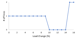
Figure 2: Number of lines switched off with different load levels.

We uniformly increase the loading condition, starting from the nominal value, of case30_ieee instance, and observe the number of lines that are switched off. As shown in Figure 2, the number of off lines first decreases, and then increases. This is because when the load is at the lower levels, some lines are redundant and are switched off to save costs. However, when the load is very high and the network is congested, lines are switched off to avoid congestion. As suggested in [5], it would be beneficial to solve the ACOTS problem frequently to obtain optimal line switching decisions for different load profiles.

VI-C Lifted cycle constraints for ACOPF-QC

TABLE II: Comparing optimality Gaps (%) for “E” and “EC” relaxations for ACOPF-QC.

Test Case	E	EC
case3_lmbd_sad	1.38	1.31
case14_ieee_sad	19.16	13.10
case24_ieee_rts_sad	2.74	2.20
case57_ieee_sad	0.32	0.25
case73_ieee_rts_sad	2.37	1.80
case240_pserc_sad	4.34	4.24
case2383wp_k_sad	1.91	1.88
case3_lmbd_api	4.53	3.85
case24_ieee_rts_api	11.02	10.88
case73_ieee_rts_api	9.52	9.31
case179_goc_api	5.86	5.75

We also add the linearized lifted cycle constraints (including the novel ones we derived) to the ACOPF-QC relaxation, This happens to be the special case of the ACOTS-QC with all the lines of the network swithced on. These cycle constraints are linearized using the strong extreme-point representation, which is also new. We experiment with “TYP”, “SAD” and “API” cases with up to 2869 buses (102 cases in total), and observe improvements of optimality gaps in several instances. We report cases with greater than 0.03% improvement in objectives in Table II. The results show that, for ACOPF-QC the lifted cycle constraints are more useful in tightening “SAD” and “API” instances, and for smaller-size test cases.

VII Conclusion

In this paper, we strengthen the on/off QC relaxation of the ACOTS model by the extreme-point representation technique, several valid inequalities added via branch-and-cut, and the OBBT algorithm. Experiments on PGLib instances show that the strengthened ACOTS-QC formulation significantly improves lower bounds in several instances, especially for small angle-difference instances and congested instances. Our proposed lifted cycle constraints improve bounds of ACOTS-QC as well as ACOPF-QC relaxations.

Considering large-scale grids, operated in a close-to-real-time fashion, ACOTS is still a very hard problem to solve with optimality guarantees. As the line switching decisions are sensitive to load changes, it would be helpful to develop stochastic programming models that provide more robust solutions. To address scaling issues, it would be useful to (i) balance the trade-off between run time and tighter formulations and (ii) develop faster decomposition-based distributed algorithms.

Appendix

A. Proof of Theorem III.1

First, we prove that ${\rm conv}(H^{0}\cup H^{1})\subseteq H$. For any $\eta^{0}\in H^{0}$, $\eta^{0}$ satisfies constraints in (7) when $z_{ij}=0$. Similarly, for any $\eta^{1}\in H^{1}$, $\eta^{1}$ satisfies constraints in (7) when $z_{ij}=1$. Thus, $H^{0}\cup H^{1}\subseteq H$. Since $H$ contains only linear constraints and is thus convex, we have ${\rm conv}(H^{0}\cup H^{1})\subseteq H$.

Next, we prove that $H\subseteq{\rm conv}(H^{0}\cup H^{1})$. Let $\eta^{*}\in H$. If $z^{*}_{ij}=0$, then $\eta^{*}\in H^{0}$, and if $z^{*}_{ij}=1$, then $\eta^{*}\in H^{1}$. When $z^{*}_{ij}\in(0,1)$, we define the following variables:

$$\eta_{0}^{*}=\left(0,0,\cdots,0,\frac{v_{i}^{*}-\sum_{k=1}^{8}\lambda^{c*}_{ij,k}\boldsymbol{\xi}_{1}^{k}}{1-z_{ij}^{*}},\frac{v_{j}^{*}-\sum_{k=1}^{8}\lambda^{c*}_{ij,k}\boldsymbol{\xi}_{2}^{k}}{1-z_{ij}^{*}}\right)$$

$$\eta_{1}^{*}=\Bigg{(}\frac{w^{R*}_{ij}}{z^{*}_{ij}},\frac{w^{I*}_{ij}}{z^{*}_{ij}},\frac{c^{*}_{ij}}{z^{*}_{ij}},\frac{s^{*}_{ij}}{z^{*}_{ij}},\frac{\lambda^{c*}_{ij,1}}{z^{*}_{ij}},\cdots,\frac{\lambda^{c*}_{ij,8}}{z^{*}_{ij}},\frac{\lambda^{s*}_{ij,1}}{z^{*}_{ij}},\cdots,\frac{\lambda^{s*}_{ij,8}}{z^{*}_{ij}},$$

$$\hskip 28.45274pt1,\sum_{k=1}^{8}\frac{\lambda^{c*}_{ij,k}}{z^{*}_{ij}}\boldsymbol{\xi}^{k}_{1},\sum_{k=1}^{8}\frac{\lambda^{c*}_{ij,k}}{z^{*}_{ij}}\boldsymbol{\xi}^{k}_{2}\Bigg{)}$$

Next, we prove that $\eta_{0}^{*}\in H^{0}$ and $\eta_{1}^{*}\in H^{1}$. Because of (7b), we have $(1-z^{*}_{ij})\boldsymbol{\underline{v}}_{i}\leqslant v_{j}^{*}-\sum_{k=1}^{8}\lambda^{c*}_{ij,k}\boldsymbol{\xi}_{2}^{k}\leqslant(1-z^{*}_{ij})\boldsymbol{\overline{v}}_{i}$. Thus, $\frac{v_{i}^{*}-\sum_{k=1}^{8}\lambda^{c*}_{ij,k}\boldsymbol{\xi}_{1}^{k}}{1-z_{ij}^{*}}\in[\boldsymbol{\underline{v}}_{i},\boldsymbol{\overline{v}}_{i}]$. Similarly, $\frac{v_{j}^{*}-\sum_{k=1}^{8}\lambda^{c*}_{ij,k}\boldsymbol{\xi}_{2}^{k}}{1-z_{ij}^{*}}\in[\boldsymbol{\underline{v}}_{j},\boldsymbol{\overline{v}}_{j}]$. Therefore, $\eta_{0}^{*}\in H^{0}$.

For $\eta_{1}^{*}$, $\frac{w^{R*}_{ij}}{z^{*}_{ij}}=\sum_{k=1}^{8}\frac{\lambda^{c*}_{ij,1}}{z^{*}_{ij}}(\boldsymbol{\xi}_{1}^{k},\boldsymbol{\xi}_{2}^{k},\boldsymbol{\xi}_{3}^{k})$ because $w^{R*}_{ij}=\sum_{k=1}^{8}\lambda^{c*}_{ij,1}(\boldsymbol{\xi}_{1}^{k},\boldsymbol{\xi}_{2}^{k},\boldsymbol{\xi}_{3}^{k})$ and $z^{*}_{ij}\in(0,1)$. Similarly, it can be proved that $\eta_{1}^{*}$ satisfies constraints (7a), (7f), (7h), and (8c). For constraint (8a), the first equation follows directly from the definition of $\eta_{1}^{*}$, and the second equality is correct because the validity of (7b) and (7c) for $\eta^{*}$ indicates that $\sum_{k=1}^{8}\lambda^{s*}_{ij,k}\boldsymbol{\gamma}^{k}_{1}+(1-z^{*}_{ij})\boldsymbol{\underline{v}}_{i}\leqslant\sum_{k=1}^{8}\lambda^{c*}_{ij,k}\boldsymbol{\xi}^{k}_{1}+(1-z^{*}_{ij})\boldsymbol{\underline{v}}_{i}$ and $\sum_{k=1}^{8}\lambda^{s*}_{ij,k}\boldsymbol{\gamma}^{k}_{1}+(1-z^{*}_{ij})\boldsymbol{\overline{v}}_{i}\geq\sum_{k=1}^{8}\lambda^{c*}_{ij,k}\boldsymbol{\xi}^{k}_{1}+(1-z^{*}_{ij})\boldsymbol{\overline{v}}_{i}$, thus $\sum_{k=1}^{8}\lambda^{c*}_{ij,k}\boldsymbol{\xi}^{k}_{1}=\sum_{k=1}^{8}\lambda^{s*}_{ij,k}\boldsymbol{\gamma}^{k}_{1}\Rightarrow\sum_{k=1}^{8}\frac{\lambda^{c*}_{ij,k}}{z^{*}_{ij}}\boldsymbol{\xi}^{k}_{1}=\sum_{k=1}^{8}\frac{\lambda^{s*}_{ij,k}}{z^{*}_{ij}}\boldsymbol{\gamma}^{k}_{1}$, which means $\eta_{1}^{*}$ satisfies the second equality in (8a). With similar arguments, $\eta_{1}^{*}$ is also feasible for (8b). Therefore, $\eta_{1}^{*}\in H^{1}$.

Now note that $\eta^{*}=(1-z^{*}_{ij})\eta_{0}^{*}+z^{*}_{ij}\eta_{1}^{*}$, which means $H\subseteq{\rm conv}(H^{0}\cup H^{1})$.

References

- [1] H. Glavitsch, “State of the art review: Switching as means of control in the power system,” Int. J. Electr. Power & Energy Syst., vol. 7, no. 2, pp. 92–100, 1985.
- [2] K. W. Hedman, R. P. O’Neill, E. B. Fisher, and S. S. Oren, “Optimal transmission switching-sensitivity analysis and extensions,” IEEE Trans. on Power Systems, vol. 23, no. 3, pp. 1469–1479, 2008.
- [3] B. Kocuk, S. S. Dey, and X. A. Sun, “New formulation and strong MISOCP relaxations for AC optimal transmission switching problem,” IEEE Trans. Power Syst., vol. 32, no. 6, pp. 4161–4170, 2017.
- [4] K. W. Hedman, S. S. Oren, and R. P. O’Neill, “A review of transmission switching and network topology optimization,” in 2011 IEEE Power and Energy Soc. Gen. Meet. IEEE, 2011, pp. 1–7.
- [5] E. B. Fisher, R. P. O’Neill, and M. C. Ferris, “Optimal transmission switching,” IEEE Trans. Power Syst., vol. 23, no. 3, pp. 1346–1355, 2008.
- [6] B. Kocuk, H. Jeon, S. S. Dey, J. Linderoth, J. Luedtke, and X. A. Sun, “A cycle-based formulation and valid inequalities for DC power transmission problems with switching,” Oper. Res., vol. 64, no. 4, pp. 922–938, 2016.
- [7] C. Coffrin, H. L. Hijazi, K. Lehmann, and P. Van Hentenryck, “Primal and dual bounds for optimal transmission switching,” in 2014 Power Syst. Comput. Conf. IEEE, 2014, pp. 1–8.
- [8] K. Lehmann, A. Grastien, and P. Van Hentenryck, “The complexity of DC-switching problems,” arXiv preprint arXiv:1411.4369, 2014.
- [9] C. Barrows, S. Blumsack, and P. Hines, “Correcting optimal transmission switching for AC power flows,” in 2014 47th Hawaii Int. Conf. on Syst. Sci. IEEE, 2014, pp. 2374–2379.
- [10] E. A. Goldis, X. Li, M. C. Caramanis, B. Keshavamurthy, M. Patel, A. M. Rudkevich, and P. A. Ruiz, “Applicability of topology control algorithms (TCA) to a real-size power system,” in 2013 51st Annu. Allerton Conf. on Commun., Control, and Comput. (Allerton). IEEE, 2013, pp. 1349–1352.
- [11] R. A. Jabr, “Radial distribution load flow using conic programming,” IEEE Trans. Power Syst., vol. 21, no. 3, pp. 1458–1459, 2006.
- [12] C. Coffrin, H. L. Hijazi, and P. Van Hentenryck, “The QC relaxation: A theoretical and computational study on optimal power flow,” IEEE Trans. Power Syst., vol. 31, no. 4, pp. 3008–3018, 2016.
- [13] X. Bai, H. Wei, K. Fujisawa, and Y. Wang, “Semidefinite programming for optimal power flow problems,” Int. J. Electr. Power Energy Syst., vol. 30, no. 6-7, pp. 383–392, 2008.
- [14] H. Hijazi, C. Coffrin, and P. Van Hentenryck, “Convex quadratic relaxations for mixed-integer nonlinear programs in power systems,” Math. Prog. Comput., vol. 9, no. 3, pp. 321–367, 2017.
- [15] K. Bestuzheva, H. Hijazi, and C. Coffrin, “Convex relaxations for quadratic on/off constraints and applications to optimal transmission switching,” INFORMS J. Comput., vol. 32, no. 3, pp. 682–696, 2020.
- [16] B. Kocuk, S. S. Dey, and X. A. Sun, “Strong SOCP relaxations for the optimal power flow problem,” Oper. Res., vol. 64, no. 6, pp. 1177–1196, 2016.
- [17] H. Nagarajan, M. Lu, S. Wang, R. Bent, and K. Sundar, “An adaptive, multivariate partitioning algorithm for global optimization of nonconvex programs,” J. Global. Opt., vol. 74, no. 4, pp. 639–675, 2019.
- [18] K. Sundar, H. Nagarajan, S. Misra, M. Lu, C. Coffrin, and R. Bent, “Optimization-based bound tightening using a strengthened QC-relaxation of the optimal power flow problem,” arXiv preprint: 1809.04565, 2018.
- [19] C. Coffrin, R. Bent, K. Sundar, Y. Ng, and M. Lubin, “PowerModels.jl: An open-source framework for exploring power flow formulations,” in 2018 Power Syst. Comput. Conf. (PSCC), June 2018, pp. 1–8.
- [20] J. A. Taylor, Convex optimization of power systems. Cambridge University Press, 2015.
- [21] K. Purchala, L. Meeus, D. Van Dommelen, and R. Belmans, “Usefulness of DC power flow for active power flow analysis,” in IEEE Power Eng. Soc. General Meeting, 2005. IEEE, 2005, pp. 454–459.
- [22] M. Lu, H. Nagarajan, R. Bent, S. D. Eksioglu, and S. J. Mason, “Tight piecewise convex relaxations for global optimization of optimal power flow,” in Power Syst. Comput. Conf. IEEE, 2018, pp. 1–7.
- [23] S. Ceria and J. Soares, “Convex programming for disjunctive convex optimization,” Math. Prog., vol. 86, no. 3, pp. 595–614, 1999.
- [24] H. Nagarajan, K. Sundar, H. Hijazi, and R. Bent, “Convex hull formulations for mixed-integer multilinear functions,” in AIP Conf. Proc., vol. 2070, no. 1. AIP Publishing LLC, 2019, p. 020037.
- [25] M. Lu, H. Nagarajan, E. Yamangil, R. Bent, S. Backhaus, and A. Barnes, “Optimal transmission line switching under geomagnetic disturbances,” IEEE Trans. Power Syst., vol. 33, no. 3, pp. 2539–2550, 2017.
- [26] B. Kocuk, S. S. Dey, and X. A. Sun, “Matrix minor reformulation and SOCP-based spatial branch-and-cut method for the AC optimal power flow problem,” Math. Prog. Comput., vol. 10, no. 4, pp. 557–596, 2018.
- [27] C. Chen, A. Atamtürk, and S. S. Oren, “Bound tightening for the alternating current optimal power flow problem,” IEEE Trans. on Power Systems, vol. 31, no. 5, pp. 3729–3736, 2015.
- [28] S. Gopinath, H. Hijazi, T. Weisser, H. Nagarajan, M. Yetkin, K. Sundar, and R. Bent, “Proving global optimality of ACOPF solutions,” Electr. Power Syst. Res., vol. 189, p. 106688, 2020.
- [29] S. Babaeinejadsarookolaee, A. Birchfield, R. D. Christie, C. Coffrin, C. DeMarco, R. Diao, M. Ferris, S. Fliscounakis, S. Greene, R. Huang et al., “The power grid library for benchmarking AC optimal power flow algorithms,” arXiv preprint arXiv:1908.02788, 2019.
- [30] O. Kroger, C. Coffrin, H. Hijazi, and H. Nagarajan, “Juniper: an open-source nonlinear branch-and-bound solver in julia,” in Internation. Conf. Integr. Constraint Program., Artif. Intell., Oper. Res. Springer, 2018, pp. 377–386.
- [31] A. Wachter and L. T. Biegler, “On the implementation of an interior-point filter line-search algorithm for large-scale nonlinear programming,” Math. Prog., vol. 106, no. 1, pp. 25–57, 2006.