Dissipation as a resource for Quantum Reservoir Computing

Abstract

Dissipation induced by interactions with an external environment typically hinders the performance of quantum computation, but in some cases can be turned out as a useful resource. We show the potential enhancement induced by dissipation in the field of quantum reservoir computing introducing tunable local losses in spin network models. Our approach based on continuous dissipation is able not only to reproduce the dynamics of previous proposals of quantum reservoir computing, based on discontinuous erasing maps but also to enhance their performance. Control of the damping rates is shown to boost popular machine learning temporal tasks as the capability to linearly and non-linearly process the input history and to forecast chaotic series. Finally, we formally prove that, under non-restrictive conditions, our dissipative models form a universal class for reservoir computing. It means that considering our approach, it is possible to approximate any fading memory map with arbitrary precision.

1 Introduction

Quantum science holds promise to revolutionize the technological perspectives in fields such as computing [1, 2], communication [3], sensing [4], or cryptography [5]. In particular, the introduction of quantum logic allows the development of algorithms that outperform the corresponding classical ones [6, 7, 8, 9, 10], with broad and interdisciplinary applications in chemistry [11], finance [12, 13] and machine learning [14]. Still, the experimental implementation of these algorithms is a challenging task with state-of-the-art technology [15, 16]. Currently available devices are mostly relying on a few (up to hundreds) noisy qubits, an obstacle to overcome to achieve a quantum advantage in ‘real world’ computation problems or quantum error correction.

A common problem is that dissipation, caused by the interaction between qubits and the external environment, produces decoherence phenomena that hinder fragile quantum resources. Dissipation, however, can be turned into a positive computational resource in some cases as for dissipation engineering, which exploits the system-environment interaction as an integral part of the computation process [17] and for quantum memories [18]. Applications range from quantum control [19] to non-equilibrium quantum thermodynamics [20, 21], quantum biology [22] or quantum synchronization [23, 24]. The aim of this work is to establish the beneficial effect of tunable dissipation on quantum machine learning and, in particular, on the field of quantum reservoir computing (QRC) [25].

Reservoir computing (RC) is a machine learning method rooted in Recurrent Neural Networks and is particularly suited for time series processing [26]. Classical RC was initially proposed as Liquid State Machines [27] and Echo State Networks [28] and later generalized to include a broad spectrum of physical implementations [29]. Major advantages of RC are the easiness of the training process, which only requires a linear regression optimization, instead of the gradient descent procedures of traditional neural networks, and to be multitasking. RC is now well-established as a powerful analog neuromorphic method in classical machine learning. Successful experimental realizations of temporal processing with RC and applications have been reported in the last years, including electronic, spintronic, and photonic systems [30, 31, 32, 33].

Recently, this supervised machine learning approach has been proposed in quantum substrates to solve both classical and quantum tasks [25], in platforms as diverse as spin networks [34, 35, 36, 37, 38, 39], fermionic setups [40, 41], continuous-variable bosonic oscillators [42, 43, 44], superconducting qubits quantum computers [45, 46, 47] and photonic integrated circuits [48]. The main motivation for this burgeoning interest is that the superposition principle allows quantum reservoirs to reach an exponential advantage over the classical ones in terms of the number of degrees of freedom. Evidence of this feature has been observed and quantified in QRC through the Information Processing Capacity [49] with spins [38] and with Gaussian networks as well [43].

In spite of the variety of dynamical systems that can serve RC purposes, there are some key features needed for temporal series processing in this architecture (formally defined in Sec. 5). In a nutshell, the system is required to store some past input information (fading memory) and to forget its initial conditions (echo state property). For quantum RC, it is known that the presence of dissipation is a necessary feature [34, 36] and, consequently, all the proposed QRC frameworks contain some dissipation.

The pioneering work of Fuji and Nakajima (FN) is based on a spin-network QRC scheme [34] and a discrete erase-and-write map. This evolution can be also realized via a local dissipation on the input nodes modeled by a Lindblad master equation, as shown in the next section. An alternative paradigm for QRC is based on the presence of engineered losses for each of the spin nodes, giving rise to continuous dissipation (CD), and on a continuous input-driving obtained by tuning an external magnetic field. We will show that the degree of adaptability of such a tailored dissipation allows the system to optimize its performance according to the task faced, thus outperforming the FN model, where the control over dissipation is very low. Furthermore, we will demonstrate that the CD model achieves universal QRC, which means that any generic task to be solved with RC can be arbitrarily well approximated by considering only these kinds of models.

The paper is structured as follows: in Sec. 2, we will review the FN model and introduce the CD one; in Sec. 3.1, we will analyze the memory properties of such models while in Sec. 3.2 we will test them in time-series forecasting tasks; in Sec. 4, we will compare the strategy to add dissipation on previously presented QRC models with our CD proposal; in Sec. 5 we will present the proof of universality for the CD model; finally, conclusions are given in Sec. 6.

2 Quantum reservoirs

According to the RC theory, a general model of a reservoir must fulfill some necessary conditions to operate. One is the echo state property condition, which consists in the disappearance of the initial condition’s dependence of the reservoir dynamics over time [50]. This is a necessary feature because otherwise, the training phase should also account for the initial state choice, making the whole procedure inefficient. Furthermore, a proper RC system requires fading memory to process the information of a time series without needing an infinite amount of physical resources [51]. Therefore, in the quantum case, dissipation is a crucial feature to satisfy these two conditions [36]. Finally, a RC model also needs to be able to discriminate different input sequences in order to adapt its behavior to the particular problem of interest [52]. We will formalize and contextualize all these features for our case study in Sec. 5. In this section, we will consider three different quantum reservoir computers focusing on the role played by dissipation in their functioning and performance. In all the cases, we will consider spin network-like reservoir systems, with their output layer being given by a linear combination of local and/or global observables.

Let us start our discussion by recalling the first model of QRC introduced by Fuji and Nakajima (FN) in Ref. [34] and based on a transverse-field Ising model characterized by the Hamiltonian

$$H=\sum_{i<j}^{N}J_{ij}\sigma_{i}^{x}\sigma_{j}^{x}+h\sum_{i=1}^{N}\sigma_{i}^{z},$$ (1)

where the $i,j$ label the sites of the network, $\sigma_{i}^{a}$ $(a=x,y,z)$ are the Pauli matrices acting on the $i$-th site, $h$ is the value of the magnetic field and $J_{ij}$ is the spin-spin coupling following a uniform distribution in a pre-determined interval $[-J_{s},J_{s}]$. We will consider real input sequence of length $M$, $\{s_{k}\}_{k=1}^{M}$, and rescaled, such that $s_{k}\in[0,1]$ $\forall k$. The FN updating rule of the reservoir is obtained by feeding the input to the state of one qubit of the network, for the sake of the definiteness we say the first one. In particular, the state of the first qubit is prepared in an input-dependent coherent superposition $\rho^{(1)}_{k}=\ket{\psi_{s_{k}}}\bra{\psi_{s_{k}}}$ where $\ket{\psi_{s_{k}}}=\sqrt{1-s_{k}}\ket{0}+\sqrt{s_{k}}\ket{1}$ (see [53] for a discussion of this and different encoding effects). Then, the system unitarily evolves for a certain interval of time $\Delta t$, only following the dynamics generated by the Hamiltonian $H$. The complete update rule is:

$$\rho_{k+1}=e^{-iH\Delta t}\rho_{k+1}^{(1)}\otimes\Tr_{(1)}\{\rho_{k}\}e^{iH\Delta t}$$ (2)

where $\Tr_{(1)}\{\cdot\}$ is the partial trace over the first qubit and $e^{-iH\Delta t}$ is the time evolution operator, assumed as unitary between the input injections. Still, the map (2) exhibits dissipation and decoherence and this occurs instantaneously at each input injection (as modeled by the partial trace).

A natural way to experimentally realize such injection on a NISQ device consists in realizing a measurement on the first spin and, subsequently, setting its state with a quantum gate conditioned by its outcome. In digital implementations like the IBM quantum computer, the reset of qubits after a measure is a recently implemented feature [54] even if it is rather slow and then susceptible to uncontrollable decoherence [55]. Let us consider instead an alternative QRC approach characterized by interactions with an external environment under Markovian conditions. The most general time evolution of a density matrix is described by the Gorini-Kossakowski-Sudarshan-Lindblad (GKLS) Master Equation [56, 57, 58]:

$$\dot{\rho}=\mathcal{L}[\rho]\equiv-i[H,\rho]+\sum_{i}\gamma_{i}(L_{i}\rho L_{i}^{\dagger}-\frac{1}{2}\{L_{i}^{\dagger}L_{i},\rho\})$$ (3)

where $\{\gamma_{i}\}$ are the decay rates of the qubits in each external environment and the operators $\{L_{i}\}$, called jump operators, identify the environment action on the qubits. In Eq. (3), we identify unitary $\mathcal{U}$ and dissipative $\mathcal{D}$ superoperators:

$$\dot{\rho}=(\mathcal{U}+\mathcal{D})[\rho]$$

with $\mathcal{U}[\rho]=-i[H,\rho]$ and $\mathcal{D}[\rho]$ equal to the remaining (Lindbladian) term. We will consider dissipation leading to local losses (i.e. independent losses at each of the $N$ reservoir nodes) modeled by N jump operators $L_{i}=\sigma_{i}^{-}\equiv\frac{1}{2}(\sigma_{i}^{x}-i\sigma_{i}^{y})$. We notice that this model adequately accounts for Markovian dissipation in independent baths whenever the interaction between reservoir nodes is weak (for a more accurate discussion see [59]). Furthermore, protocols to engineer a Lindbladian with these characteristics are also known [17]. In Appendix A, we show how dissipation acting locally on the first oscillator leads to an evolution that is able to reproduce the FN map (2).

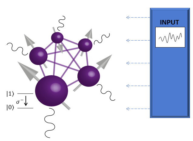
Let us now introduce a different model of quantum reservoir computing characterized by continuous dissipation (CD) and where the input is injected into the system through temporal driving, varying a Hamiltonian parameter. We consider, in particular, a variable magnetic field modulated in the x-direction into the Hamiltonian (1):

$$H^{{}^{\prime}}=\sum_{i<j}^{N}J_{ij}\sigma_{i}^{x}\sigma_{j}^{x}+h\sum_{i=1}^{N}\sigma_{i}^{z}+h^{\prime}(t)\sum_{i=1}^{N}\sigma_{i}^{x}.$$ (4)

The time-dependent $h^{\prime}(t)$ encodes the input time series and modifies coherently the evolution of the reservoir. For each input $s_{k}\in[0,1]$, driving persists for a certain interval $\Delta t$ according to the assignment rule $h^{\prime}_{k}(t)=h\cdot(s_{k}+1)$. As dissipation is required for QRC [36], the unitary dynamics generated by the Hamiltonian (4) will not be sufficient for our purposes. The simplest kind of dissipation we can introduce consists of adding local, uniform losses to the reservoir nodes ($\gamma_{i}=\gamma$ $\forall i$). We will see that the decay rate $\gamma$ strongly affects the memory and computational properties of the system. During each time interval, the reservoir dynamics is governed by

$$\dot{\rho}=-i[H_{k}^{\prime},\rho]+{\cal D}_{L}[\rho]$$ (5)

where the local (L) dissipator is given by ${\cal D}_{L}[\rho]\equiv\gamma\sum_{i}(\sigma_{i}^{-}\rho\sigma_{i}^{+}-\frac{1}{2}\{\sigma_{i}^{+}\sigma_{i}^{-},\rho\})$ and where $H_{k}^{\prime}=H^{\prime}(h^{\prime}_{k})$. Therefore, in this case, $\mathcal{U}$ and $\mathcal{D}_{L}$ are functions of the input and $\gamma$ respectively and the updating rule of the reservoir is:

$$\rho_{k+1}=e^{[\mathcal{U}(s_{k+1})+\mathcal{D}_{L}(\gamma)]\Delta t}\rho_{k}\equiv e^{\bar{\mathcal{L}}(s_{k+1})\Delta t}\rho_{k}$$ (6)

where the specific choice of continuous-dissipation and input-driven dynamics is distinguished by the bar in $\bar{\mathcal{L}}$. A schematic representation of this CD model is shown in Fig. 1.

Figure 1: Schematic picture of the CD model proposed in Eq. (6): spin network with uniform losses in which the input is uniformly injected in the network nodes through a time-dependent magnetic field.

3 Computational benchmark tasks

We now proceed to evaluate numerically the computing performance of the FN and CD models. We will tackle two families of benchmark tasks usually present in the RC literature, namely memory and forecasting tasks. We set the reservoir to $N=5$ spins, which already guarantees a big enough density matrix, with a number of elements $\sim 4^{5}$, while being QRC tasks computationally accessible in a standard desktop computer. For the readout layer, we choose a linear combination of the expectation values of Pauli strings with length one ($\langle\sigma_{i}^{a}\rangle$) and two ($\langle\sigma_{i}^{a}\sigma_{j}^{a}\rangle$), with $a=x,y,z$, and $1\leq i,j\leq N$, $i\neq j$. Altogether, the output layer is made of $45$ nodes which are the parameters determined during the training phase.

3.1 Memory tasks

In this section, we will present the performances of tasks related to the capacity of the systems to linearly and non-linearly process the memory of previous inputs, starting with a linear memory test: the short-term memory task (STM) [60]. Following the standard procedure, the input originates from a random uniform distribution in the interval $[0,1]$ and the expected target at each time step ($y_{k}$) is to reproduce the previous input for a given delay $\tau$

$$y_{k}=s_{k-\tau}.$$

Indeed, the STM task measures the ability of a system to store information about the input received a certain number $\tau$ of time steps in the past, being an indicator of linear memory. The metric chosen to evaluate all the presented memory tasks is the capacity:

$$C=\frac{\mathrm{cov}^{2}(\textbf{y},\bar{\textbf{y}})}{\sigma(\textbf{y})^{2}\sigma(\bar{\textbf{y}})^{2}}$$

where y and $\bar{\textbf{y}}$ are respectively the time series of the targets and the predictions, $\mathrm{cov}(\cdot)$ is the covariance and $\sigma(\cdot)$ is the standard deviation. The coefficient $C$ ranges between $C=0$ (complete mismatch of the predictions) and $C=1$ (perfect accuracy).

Our analysis encompasses a coarse-grained exploration to optimize the hyperparameters of the models for all the tasks discussed in this paper. Working in the units of $J_{s}$, the degrees of freedoms $h$, $\Delta t$, and $\gamma$ are varied by orders of magnitude taking values from the following set: $\{0.01,0.1,1,10\}$. For every possible combination of these hyperparameters, we have simulated 100 different random pairs of coupling sets $\{J_{ij}\}$ and input sequences and we took the metric average over them as the representative value. Finally, the combination with the average of maximum performance in the given task has been considered optimal.

The results of the STM task, specifying the values of the hyperparameters, are shown in Fig. 2 (a). In general, for different orders of delay, the optimal set of free parameters varies for all the models, which makes it evident that the learning capability of the reservoir is strongly influenced by the choice of such hyperparameters. We found that FN reservoir memory is maximized for $h=0.1$ and $\Delta t=10$ when $\tau<\tau_{1}^{*}=5$ while in the complementary case $\Delta t$ changes to 1. For our proposal (CD model (6)) four different optimal sets have been found. Indicating the free hyperparameters through a triple of the form $(h,\Delta t,\gamma)$, for the regions of delay $\tau<\tau_{1}=2$, $\tau_{1}\leq\tau<\tau_{2}=6$, $\tau_{2}\leq\tau<\tau_{3}=16$ and $\tau_{3}\leq\tau\leq 20$ the optimal sets are respectively (0.1, 10, 1), (0.01, 10, 0.1), (0.01, 10, 0.01) and (0.01, 1, 0.1). For all the values of the delay, the CD dynamical map (6) is able to reach better performances than the FN model. This suggests that the tunable damping rate introduced in the dynamics, which is an extra free hyperparameter with no equivalent in the FN map, allows us to have more control over the linear dependence from the past injected input.

Another well-established and challenging benchmark test studied in the context of RC is the nonlinear auto-regressive moving average (NARMA) task, first introduced in the context of RNNs [61]. This task, beyond requiring linear memory, also adds the requirement of non-linear memory, and its formulation depends on a given order of delay $n$. At any time step, the NARMA$(n)$ target is

$$y_{k} = 0.3y_{k-1}+0.05y_{k-1}\sum_{j=1}^{n}y_{k-j}$$ (7)

$$+ 1.5s_{k-n}s_{k-1}+0.1.$$

Figure 2: Performance evaluation of different memory tasks for the FN model described in Eq. (2) (red) and for CD in Eq. (6) (blue). Capacity for STM task (a), NARMA task (b), and parity check (c). Optimized hyperparameters as specified in the main text for the STM task, while for NARMA and parity check the hyperparameters are also optimized but not reported, being not relevant for the conclusions. A number of 1000 time steps have always been used for the washout, training, and evaluation phase. In all the plots the shadow regions cover one standard deviation taken as statistical error over the 100 random realizations of spin coupling values for the Hamiltonians of the systems $\{J_{ij}\}$.

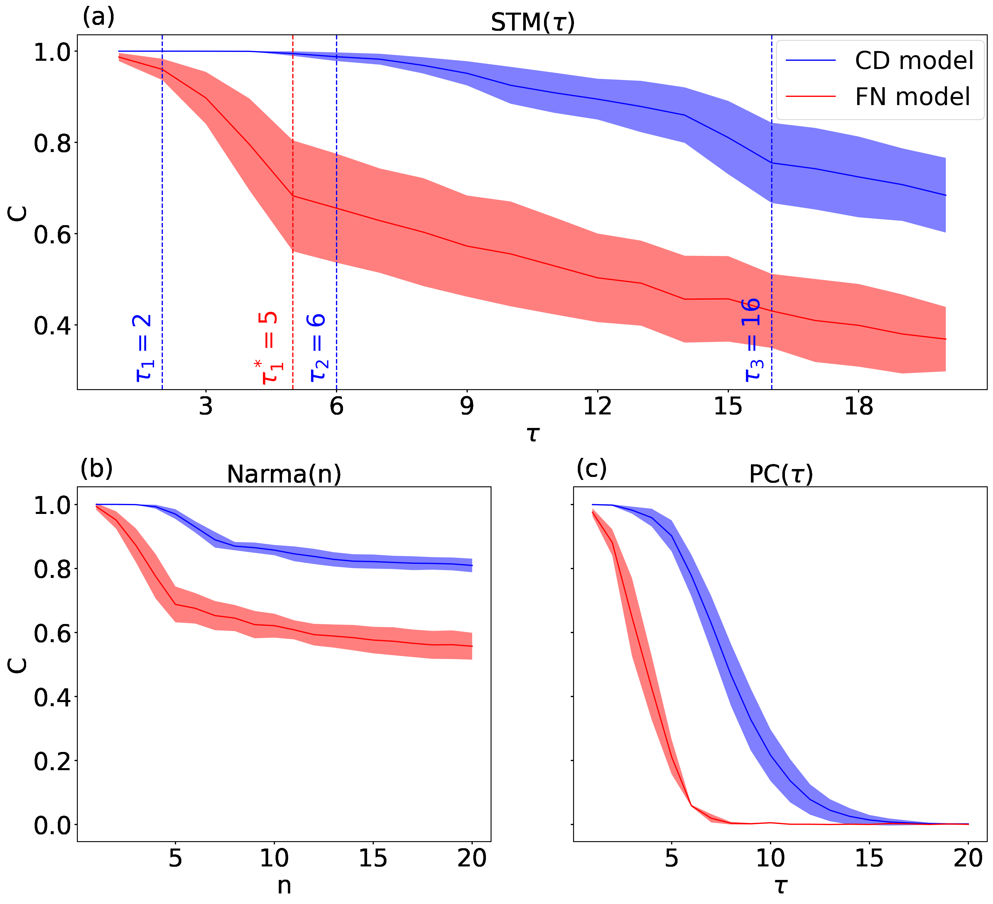
As usual, to prevent divergences until an order of delay equal to $20$, it is necessary to define the target of the task rescaling the input in the interval $[0,0.02]$. The NARMA task performances, for both systems, are shown in Fig. 2 (b). Also in this case the results show that the CD model performs better than the FN one, broadening our conclusions about the STM task, also for a target that includes some nonlinearity.

We conclude our analysis of the memory properties considering the parity-check task [62]. In this case, we work with a binary random input sequence $s_{k}\in\{0,1\}$. The desired output for a delay $\tau$ is given by

$$y_{k}=\sum_{j=1}^{\tau}s_{k-j}\mod 2.$$

This task is strictly non-linear and, in fact, for a delay equal to $\tau$, it has the degree of nonlinearity of a monomial of degree $\tau$ of the previous inputs. In order to reach performances not negligible for $\tau>1$, we have introduced in both the QRC models the time multiplexing, considering $V=15$ virtual nodes. It means that, for each input injection, during the evolution time $\Delta t$, the observables in the readout have been collected not only in the final time but in $V$ equidistant times of the dynamics [34, 38]. The optimal performances for this task are shown in Fig. 2 (c). Even for this fully nonlinear task, the CD model outperforms the FN one. Therefore, from the results obtained, we can conclude that the CD model, with the introduction of the new tunable dissipation $\gamma$, reaches better performances for all the memory tasks considered. The proposed approach of continuous dissipation allows indeed to achieve better control of the dynamical system response. We also remark that the optimal results for the FN model found are in agreement with the ones theorized in [63], where the role of the QRC performance in connection with dynamical phase transitions was discussed.

3.2 Time series forecasting

Apart from memory tasks, RC is especially suited for chaotic time series forecasting. A popular benchmark application is the prediction of the well-known Mackey-Glass (MG) dynamical evolution [64]. The target obeys the following differential equation:

$$\dot{s}(t)=-0.1s(t)+\frac{0.2s(t-\tau)}{1+s(t-\tau)^{10}}$$ (8)

being in the chaotic regime for $\tau=17$, as reported in previous works on time series forecasting [65, 66].

During the training phase, we have injected, as input sequence into the system, the numerical solutions of Eq. (8) sampled with a time resolution $t_{r}=3$ (see [67] for more details) and with input values rescaled in the interval $[0,1]$. The readout weights were trained to solve the one-step-ahead prediction task:

$$y_{k}=s_{k+1}$$

During the evaluation phase, the systems have been left to evolve in an autonomous way taking, at each time step, their previous prediction as a current input.

Here, we can distinguish between the short-term (weather-like) forecast of the dynamical trajectories and the long-term (climate-like) forecast of the chaotic attractor [68]. We first show in Fig. 3 (a) that both the CD and FN models are able to reproduce the shape of the chaotic attractor of the Mackey-Glass time series (climate-like forecast). In order to perform a quantitative analysis, we have also tested the capabilities of the systems to predict the oscillations of the target trajectory from the start of the autonomous phase (weather-like forecast). The metrics used to evaluate the performances for this task was the mean squared error:

$$MSE=\frac{\sum_{i=1}^{M}(\bar{y}_{i}-y_{i})^{2}}{M}$$

where the index $i$ iterates the times and $M$ is the number of points analyzed. Setting $M=150$, we were able to see differences as plotted in Fig. 3 (b). The average MSE values for the CD and FN models over these 150 samples are $8\cdot 10^{-3}$ and $5\cdot 10^{-2}$, respectively. This last result allows us to conclude that, also for the forecasting task explored here, the introduction of local losses makes it possible to achieve higher performance.

4 Dissipation maps discussion

The importance of dissipation was already pointed out in the pioneering FN reference [34]. Our analysis establishes the advantage of continuous dissipation in QRC compared to previous proposals. From the more abstract point of view of CPTP maps, we can say that the FN model of Eq. (2) can be described as a sequential map composed by a dissipation ($\Phi_{D}$) and a Hamiltonian evolution ($\Phi_{U}$): $\Phi=\Phi_{U}\circ\Phi_{D}$. A slightly different approach was taken in Refs. [46, 47] in the attempt to model the decoherent noise in a quantum circuit, where the roles of $\Phi_{U}$ and $\Phi_{D}$ were reversed: $\Phi=\Phi_{D}\circ\Phi_{U}$. The Markovian continuous-dissipation map of Eq. (6) goes beyond these proposals as dissipation and driving act in a continuous and, in general, non-factorizable way.

Interestingly, our map can approximate all these factorized ones [34, 46, 47] by a proper choice of the dissipation rates and their time dependence. Indeed, for the erase and write map of Eq. (2) this is shown in Appendix A. On the other hand, the model used in Refs. [46, 47] assumes a noise modeled by a Markovian channel $\Phi_{D}$ so that also $\Phi$ is Markovian, and in general can be written in the GKLS form (3). In conclusion, we remark that the major generality and tunability obtained with our formalism has been revealed to be useful in practical applications as shown in the performance improvements found in Sec. 3.

Figure 3: Results of the Mackey-Glass time-series prediction of the systems. In all the cases we have set 1000 points for the washout and training phase. The optimal free hyperparameters found, and fixed in the following plots, are $h=1$, $\Delta t=10$ for FN model and $h=0.1$, $\Delta t=0.1$, $\gamma=10$ for the CD model. (a) Chaotic attractor autonomous reproductions (CD and FN) in the phase space $y(t)$-$y(t-6)$ compared to the target attractor (MG) for one exemplary realization of the systems couplings $\{J_{ij}\}$. 2000 points have been used for the plots. (b) Predictions of 150 points in the autonomous phase contrasted to target values of the series averaged over 100 random realizations of the coupling values. The shadows cover one standard deviation taken as a statistical error.

5 Universality

In this section, we will prove that the CD model proposed in Eq. (6) forms a universality class for reservoir computing. In the context of QRC, universality corresponds to an approximation property and, in particular, is referred to the capability to arbitrarily well approximate any fading memory map [27, 69]. It will be shown that our proposal satisfies both the echo state property (ESP) and the fading memory property (FMP). Finally, it will be proven the separability verifying that the hypotheses of the Stone-Weierstrass theorem are fulfilled, then proving the universality.

5.1 Echo state property

The ESP refers to the capability of a reservoir to forget the initial conditions in the limit of an infinite input sequence [50]. It has been recently shown that this is equivalent to the usual definition of a unique solution in the RC literature, under some mild conditions (Theorem 1 in [70]). In our case of study, it means that given a left infinite and time-ordered input sequence $\{\cdots,s_{-1},s_{0}\}$ (where the 0-th time step corresponds to the last input) and given two different initial quantum states $\rho_{1}$ and, $\rho_{2}$, whose dynamics is driven by this sequence, the evolved states will become indistinguishable:

$$\lim_{k\to-\infty}\|\prod_{i=k}^{0}e^{\bar{\mathcal{L}}(s_{k})\Delta t}\left(\rho_{1}-\rho_{2}\right)\|=0,$$ (9)

where the limit is considered to be pointwise and $\|\cdot\|$ indicates any matrix norm (since all norms are equivalent in finite-dimensional spaces).

A sufficient condition for this relation to hold is strict contractivity (Theorem 2.2 in Ref. [71]): $||e^{\bar{\mathcal{L}}(s_{k})\Delta t}(\rho_{1}-\rho_{2})||\leq r||\rho_{1}-\rho_{2}||$ for all $s_{k}$ and any pair of states $\rho_{1}$ and $\rho_{2}$, where $0\leq r<1$. In particular, this can be ensured for Markovian maps that provide a unique stationary state for a generic input $s_{k}$, a property that our model posses according to Theorem 2 [72], setting a long enough value of $\Delta t$. More precisely, for a generic generator $\bar{\mathcal{L}}(s_{k})$, we can always define a finite mixing time, denoted as $\Delta t_{mix}$, such that if $\Delta t\geq\Delta t_{mix}$ then the map is strictly contractive and the ESP holds.

As a further observation, we estimated the $\Delta t_{mix}$ trend as the system dimensions increase. Our numerical analysis suggests that the $\Delta t_{mix}$ upper bound has an asymptotic behavior $\sim\frac{N}{\gamma}$ (see Appendix B for more details). Concluding, the mixing time of all the proposed maps $e^{\bar{\mathcal{L}}(s_{k})\Delta t}$ in addition to being finite, according to what we have observed numerically, scales efficiently with the number of qubits.

5.2 Fading memory

Considering the set of left infinite sequences of inputs belonging to the interval $[0,1]$, $K^{-}([0,1])$, the fading memory property is a condition of continuity of functionals defined on this set with a given norm. For a sequence $s\in K^{-}([0,1])$, this norm is defined starting from a generic null sequence, say $w=\{w_{k}\}_{k\geq 0}$ such that $\lim_{k\rightarrow\infty}w_{k}=0$, in the following way:

$$\|s\|_{\textit{w}}=\sup_{k\in\mathbb{Z}^{-}}|s_{k}|w_{-k},$$

where $s_{k}$ and $w_{-k}$ are respectively elements of s and w and $\mathbb{Z}^{-}$ is the set of negative integers. By definition, we say that a map has fading memory if, for any null sequence w, it is continuous in $(K^{-}([0,1]),\|\cdot\|_{\textit{w}})$. In order to prove that the model of Eq. (6) has fading memory, it is sufficient to prove that $e^{\bar{\mathcal{L}}(s_{k})\Delta t}$, with $\Delta t>\Delta t_{mix}$ to ensure the ESP, is a continuous function of $s_{k}$ according to [36] (Lemma 3). If $\bar{\mathcal{L}}(s_{k})$ is continuous then the continuity of its exponential will be a direct consequence. Let $s_{k}$,$u_{k}$ $\in[0,1]$, $\|\cdot\|_{2}$ be the Hilbert-Schmidt norm and $\rho$ be a unit density matrix belonging to $\mathbb{C}^{2^{N}\times 2^{N}}$. Then

$$\sup_{\rho}\left\|(\bar{\mathcal{L}}(s_{k})-\bar{\mathcal{L}}(u_{k}))\rho\right\|_{2}=$$

$$\sup_{\rho}\left\|(s_{k}-u_{k})\left[\sum_{i=1}^{N}\sigma_{i}^{x},\rho\right]\right\|_{2}\leq 2\cdot N\cdot|s_{k}-u_{k}|$$ (10)

where the first inequality is a consequence of the following property of the commutator: $\left\|\left[\sigma_{i}^{x},\rho\right]\right\|_{2}\leq 2\cdot\|\rho\|_{2}=2$ which can be proven expanding $\rho$ as a linear combination of Pauli strings and using their commutation rules. The last term of Eq. (10) implies continuity because it shows that an arbitrarily small distance between the two functions, let us say $\epsilon$, is reached when the distance of the two inputs is $|s_{k}-u_{k}|<\delta_{\epsilon}=\frac{\epsilon}{2N}$.

We then conclude that the family, say $\mathfrak{L}$, of functionals defined by Eq. (6), with the output layer of expected values, belongs to the set of fading memory functionals $C(K^{-}([0,1]),\|\cdot\|_{\textit{w}})$, which map input sequences into real expected values of observables.

5.3 Stone-Weierstrass theorem

The universality condition is obtained if $\mathfrak{L}$ is also a dense subset of $C(K^{-}([0,1]),\|\cdot\|_{\textit{w}})$. It implies that any fading memory map $f\in C(K^{-}([0,1]))$ can be arbitrarily well approximated by an element of $\mathfrak{L}$. Quantitatively for any $f\in C(K^{-}([0,1]))$ and for any $\epsilon>0$ exist $l\in\mathfrak{L}$ such that the following condition holds:

$$\left|f-l\right|_{\infty}=\sup_{s\in K^{-}([0,1])}\left|f(s)-l(s)\right|<\epsilon.$$

A sufficient condition to obtain this result is given by the well-known Stone-Weierstrass theorem: Let E be a compact metric space and $\mathbf{C}$(E) be the set of real-valued continuous functions defined on E. If a subalgebra A of $\mathbf{C}$(E) contains the constant functions and separates points of E, then A is dense in $\mathbf{C}$(E).

A first important observation is that the input space $(K^{-}([0,1]),\|\cdot\|_{\textit{w}})$ is a compact space according to [73] (Lemma 2) as required.

5.4 Input separability

Now we prove the separability of $\mathfrak{L}$. It means that given two sequences $s,\bar{s}\in K^{-}([0,1])$ such that $s\neq\bar{s}$ exists at least one element of $\mathfrak{L}$ able to separate them. In our context it is translated to the condition that the corresponding density matrices at the 0-th time step must be different: $\left\|\rho_{0}-\bar{\rho}_{0}\right\|\neq 0$.

It is useful at this point to show an important property of Eq. (6):

Lemma 1: Given two different inputs $s_{k}$, $u_{k}$ then the corresponding stationary states of $\bar{\mathcal{L}}(s_{k})$ and $\bar{\mathcal{L}}(u_{k})$ are different.

Proof:

We firstly give a necessary condition for a stationary state $\rho_{ss}$ which corresponds to a generator $\bar{\mathcal{L}}(s_{k})$. It is helpful to expand $\rho_{ss}$ in the basis of Pauli strings:

$$\rho_{ss}=\sum_{i_{1},\cdots,i_{N}}\Tr{\sigma^{i_{1}}\otimes\cdots\otimes\sigma^{i_{N}}\cdot\rho_{ss}}\sigma^{i_{1}}\otimes\cdots\otimes\sigma^{i_{N}}$$

where the indexes $\{i_{n}\}$ label single Pauli matrices: $i_{n}=x,y,z$ or the identity matrix, say $\sigma^{0}=\mathbb{I}$, for the Hilbert space of a single qubit. A necessary condition can be found projecting the definition of $\rho_{ss}$ (i.e. $\bar{\mathcal{L}}(s_{k})\rho_{ss}=0$) on a given Pauli string; we will consider $\sigma^{z}_{i}$:

$$\Tr{\sigma_{i}^{z}\bar{\mathcal{L}}(s_{k})\rho_{ss}}=0.$$ (11)

Observing that we can write the Lindbladian of Eq. $\eqref{eq:New_model}$ as a sum of single qubit dissipators:

$$\mathcal{D}=\gamma\sum_{i=1}^{N}d_{i}$$

where $d_{i}(\rho)=\sigma_{i}^{-}\rho\sigma_{i}^{+}-\frac{1}{2}\{\sigma_{i}^{+}\sigma_{i}^{-},\rho\}$ with $\sigma^{+}=\sigma^{-\dagger}$, its action on the single qubit Hilbert space:

$$d_{i}(\mathbb{I}) =-\sigma^{z}$$

$$d_{i}(\sigma^{z}) =-\sigma^{z}$$

$$d_{i}(\sigma^{y}) =-\frac{1}{2}\sigma^{y}$$

$$d_{i}(\sigma^{x}) =-\frac{1}{2}\sigma^{x}$$

implies the following expression for Eq. (11):

$$\gamma\cdot\alpha_{i}^{z}+\frac{\gamma}{2^{N}}-\sum_{j\neq i}J_{i,j}\cdot 2\cdot\alpha_{i,j}^{y,x}-2\cdot h\cdot(s_{k}+1)\cdot\alpha_{i}^{y}=0,$$ (12)

where $\alpha_{i}^{z}=\Tr{\sigma_{i}^{z}\rho_{ss}}$, $\alpha_{i,j}^{y,x}=\Tr{\sigma_{i}^{y}\sigma_{j}^{x}\rho_{ss}}$, $\alpha_{i}^{y}=\Tr{\sigma_{i}^{y}\rho_{ss}}$.

Considering now another generic input $u_{k}$, such that $u_{k}\neq s_{k}$, if $\rho_{ss}$ is a common stationary state of both, the following relation must be satisfied:

$$\bigl{(}\bar{\mathcal{L}}(s_{k})-\bar{\mathcal{L}}(u_{k})\bigr{)}\rho_{ss}=0,$$

implying that

$$\left[\sum_{i=1}^{N}\sigma_{i}^{x},\rho_{ss}\right]=0.$$ (13)

Equation (13) gives necessary conditions for the coefficients of $\rho_{ss}$ and, among these, it gives these relations: $\Tr{\sigma_{i}^{a}\rho_{ss}}=\alpha_{i}^{a}=0$, $\Tr{\sigma_{i}^{a}\sigma_{j}^{x}\rho_{ss}}=\alpha_{ij}^{ax}=0$ with $a=y,z$ and $1\leq i,j\leq N$. Then Eq. (12) becomes $\frac{\gamma}{2^{N}}=0$ which is not satisfied because we are assuming that $\gamma\neq 0$ in order to guarantee the ESP. As a consequence, we can conclude that Lemma 1 holds. $\blacksquare$

Another useful statement to arrive at the input separability is the following:

Lemma 2: Let $s_{k}$ and $\rho_{ss}(s_{k})$ be a generic input and its corresponding unique stationary state, let $\mathbb{P}$ be the set of the density matrices of the considered N qubits system and let $d\colon\mathbb{P}\times\mathbb{P}\to\mathbb{R}^{+}$ be the distance induced by the Hilbert-Schmidt product, then the following function $g\colon\mathbb{R}^{+}\times\mathbb{P}\to\mathbb{R}^{+},\quad(t,\rho)\mapsto d\left(e^{\bar{\mathcal{L}}(s_{k})t}\rho,\rho_{ss}(s_{k})\right)$ is bounded, its maximum $\left(d_{max}^{(s_{k})}\right)$ always exists and it is strictly decreasing in t when $t>\Delta t_{mix}$.

Proof:

We first observe that for any fixed value of the time g is a continuous function on $\mathbb{P}$. This is because it is a composition of continuous functions: the action of $e^{\bar{\mathcal{L}}(s_{k})t}$ composed to the action of the distance from a fixed point. As a consequence because $\mathbb{P}$ is a compact set and because the continuous image of a compact set is a compact set we arrive at the following relation:

$$\left.g(\mathbb{P})\right|_{t}=\left[0,d_{max}^{(s_{k})}(t)\right].$$ (14)

We observe that for the boundaries of the set of the density matrices $d_{max}^{(s_{k})}(t)\leq 2$. Considering now the action of $g$ for a fixed density matrix in $\mathbb{P}$, we know that $\left.g(t)\right|_{\rho}=d(e^{\bar{\mathcal{L}}(s_{k})t}\rho,\rho_{ss}(s_{k}))$ is strictly decreasing for all $\rho\neq\rho_{ss}(s_{k})$ if $t>\Delta t_{mix}$ as a consequence of the already mentioned strict contractivity of $e^{\bar{\mathcal{L}}(s_{k})t}$. Finally the same property must hold for $d_{max}^{(s_{k})}(t)$ while $\lim_{t\to+\infty}d_{max}^{(s_{k})}(t)=0$ and $d_{max}^{(s_{k})}(0)=2$. $\blacksquare$

We can now return to the problem of the separability in which we have the two generic different sequences $s$ and $\bar{s}$. Considering the smallest index J such as $s_{-J}\neq\bar{s}_{-J}$, applying Lemma 1 we know that two different stationary states exist: $\rho_{ss}(s_{-J})$ and $\rho_{ss}(\bar{s}_{-J})$. We define two open balls of radius r respectively centered on the two states: $B_{r}(\rho_{ss}(s_{-J}))$ and $B_{r}(\rho_{ss}(\bar{s}_{-J}))$ such that $B_{r}(\rho_{ss}(s_{-J}))\cap B_{r}(\rho_{ss}(\bar{s}_{-J}))=\emptyset$. The last condition is easily satisfied if $r<d(\rho_{ss}(s_{-J}),\rho_{ss}(\bar{s}_{-J}))/2$. In order to find an element of $\mathfrak{L}$ which separates the sequences, applying Lemma 2, we have to set $\Delta t$ into a sufficiently long value so that: $d_{max}^{(s_{-J})}(\Delta t),d_{max}^{(\bar{s}_{-J})}(\Delta t)<r$.

With this condition, it is ensured that after the applications of the two inputs the resulting states of the reservoirs will be different regardless of their states at the time-step $-J$. After this injection by hypothesis, the subsequent inputs will be the same, and necessary the corresponding states of the reservoir at the time 0 will be different because $e^{\bar{\mathcal{L}}(s_{k})t}$ is a full rank linear operator. We can in this way conclude that the input separability is satisfied.

5.5 Polynomial algebra and final considerations about the universality

Another hypothesis that must be satisfied in order to have universality is the presence of a subalgebra in $\mathfrak{L}$. Since we are working on a system that gives as output a linear combination of observables of the density matrix we have to look for a polynomial algebra. It can be obtained by adding to the family the model of Eq. $\eqref{eq:New_model}$ in spatial multiplexing. It means that we can consider V different and independent states $\{\rho^{(1)},\cdots,\rho^{(V)}\}$ whose dynamics will be lead by generators of the form of Eq. $\eqref{eq:New_model}$ with, in general, different value of the characteristic hyperparameters: $\{\bar{\mathcal{L}}_{1},\cdots,\bar{\mathcal{L}}_{V}\}$. We can write the total updating rule of the total reservoir in the following way:

$$\rho_{k+1}^{tot} =\rho^{(1)}_{k+1}\otimes\cdots\otimes\rho^{(V)}_{k+1}$$

$$=e^{\bar{\mathcal{L}}_{1}(s_{k+1})\Delta t}\cdots e^{\bar{\mathcal{L}}_{V}(s_{k+1})\Delta t}\rho^{(1)}_{k}\otimes\cdots\otimes\rho^{(V)}_{k}.$$

Considering the set of the polynomial outputs for all the single states $\{\mathcal{P}_{1},\cdots,\mathcal{P}_{V}\}$ we achieve the algebra considering as output for the reservoir a linear combination of the polynomials:

$$\mathcal{P}_{tot}=\beta_{0}+\sum_{i=1}^{V}\beta_{i}\cdot\mathcal{P}_{i}.$$

These newly added reservoirs satisfy the fading memory condition according to [36] (Lemma 5).

The only condition that remains to be proven in order to assert the Stone-Weierstrass theorem is the presence of constant functions in the family $\mathfrak{L}$ but it is trivially satisfied due to the fact that we are working with polynomial inputs. We can now conclude that $\mathfrak{L}$ is a universal class for reservoir computing.

Finally, we notice that this proof does not hold only for Eq. (6) but for a more general class of reservoirs working with a master equation. The conditions required for the generator $\mathcal{L}$ are the following: (i) it admits only one stationary state for each input $s_{k}$, (ii) it must be a continuous function of $s_{k}$, (iii) given two different generic inputs, say $s_{k}$ and $u_{k}$, the stationary states of $\bar{\mathcal{L}}(s_{k})$ and $\bar{\mathcal{L}}(u_{k})$ are also different.

6 Conclusions

In this paper, we have shown that tunable losses in external environments can be turned into a crucial factor for quantum reservoir computing, to tailor and optimize the memory capabilities of the system. In our analysis, we have compared the performances of continuous dissipation with alternative ones based on a discontinuous erasing map, as proposed by Fuji and Nakajima [34]. We have shown how a continuous dissipation strategy can be used to approximate and implement the FN model, considering local losses on one node of the reservoir network. Beyond this, we have addressed QRC based on an input-dependent generator of the dynamics $\bar{\mathcal{L}}(s_{k})$ and on the presence of Markovian dissipation. This has been modeled through a local master equation in the Lindblad form, with uniform and tunable decay rates.

Through a set of tasks commonly employed to benchmark time series processing, we have shown that the degree of tunability of the losses represents a powerful tool that allows the system to be reconfigured with respect to the specific problem under consideration. Indeed, for any task, we have found a range of values of the losses for which the performance indicators overcome the ones obtained using the FN model, both memory and forecasting temporal tasks. While a clear improvement is already achieved assuming here the simplest form of dissipation, the idea of dissipation engineering can be explored also considering non-local losses [24], as well as non-Markovian dissipation [74], opening the way to study a broader spectrum of quantum reservoir computers.

As a further major result, we have analytically shown that our model fulfills the two necessary conditions for time series processing as a reservoir computer (the echo state property and the fading memory property) proving that it forms a class of universality, approximating any fading memory map with arbitrary precision. Finally, our proof has shown that this last result is a more general feature of open quantum systems Markovian dynamics. In fact, universality is achieved if the generator of the dynamics has the following general, mild properties: for each input injection at sufficiently long $\Delta t$, it must admit only one stationary state; it must be a continuous function of the input; finally, for different inputs, the corresponding stationary states must be in turn different. This serves as the ground to explore other QRC architectures based on open quantum systems beyond the Ising model network analyzed here and including the unavoidable effect of quantum measurement [75, 76].

7 Acknowledgments

Funding acknowledged from the Spanish State Research Agency, through the QUARESC project (PID2019-109094GB-C21/AEI/ 10.13039/501100011033) and the Severo Ochoa and María de Maeztu Program for Centers and Units of Excellence in R&D (MDM-2017-0711), from CAIB through the QUAREC project (PRD2018/47), and from the CSIC Interdisciplinary Thematic Platform (PTI+) on Quantum Technologies in Spain (QTEP+). AS acknowledges funding from the CSIC hub on AI through the scholarship JAEIntroAIHUB2-19. GLG is funded by the Spanish MEF/MIU and co-funded by the University of the Balearic Islands through the Beatriz Galindo program (BG20/00085).

Appendix A Fuji-Nakajima map and Lindblad dynamics

Figure 4: Hilbert-Schmidt distance of states evolving according to the left-hand side or the right-hand side of Eq. (15), say $\rho_{A}$ and $\rho_{B}$, as a function of the amount of dissipation. Values are averaged over 100 random pairs of density matrices and inputs, respectively $\rho_{k}$ and $s_{k}$ in the formula.

In the following, we want to frame the FN model into our Markovian strategy to obtain dissipation by designing an equivalent input injection strategy. The idea is to replace the role played by the partial trace by introducing a strong loss on the first qubit and then preparing its state by applying the rotation operator

$$R_{y}(\theta_{k})=\begin{pmatrix}\cos\theta_{k}&\sin\theta_{k}\\ -\sin\theta_{k}&\cos\theta_{k}\end{pmatrix}$$

to it. More precisely the network’s damping rates will be

$$\gamma_{i}=\begin{cases}\gamma,&\mbox{if $i=1$ }\\ 0,&\mbox{otherwise}\end{cases}$$

and the input $s_{k}$ will be converted into an angle of rotation $\theta_{k}$ according to $\theta_{k}=\arccos(\sqrt{1-s_{k}})$. Accounting for the two steps, we can determine the conditions for the entire process, at each input injection, to be equivalent to the updating step of Eq. (2), i.e.,

$$R_{y}^{(1)}(\theta_{k+1})e^{\mathcal{D}_{1}\Delta t_{d}}\rho_{k}\approx\rho_{k+1}^{(1)}\otimes\Tr_{(1)}\{\rho_{k}\},$$ (15)

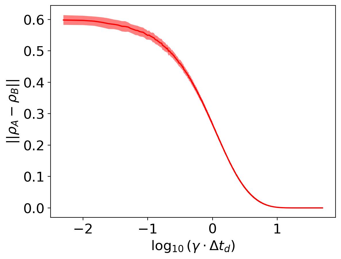
where $R_{y}^{(1)}(\theta_{k+1})$ is the gate applied to the first qubit, $\mathcal{D}_{1}$ is the dissipator acting only on the first spin, and $\Delta t_{d}$ is the dissipation time. Notice that $\Delta t_{d}$ is a time associated to the writing process not to be confused with $\Delta t$ (time between two input injections). In the FN protocol, this writing step is ideally modeled as instantaneous. As expected the stronger the effect of dissipation - larger product $\gamma\cdot\Delta t_{d}$ - the better the approximation to the FN map (2). In fact, taking the pointwise limit of $\gamma\cdot\Delta t_{d}\to+\infty$, it is straightforward to check the relation in Eq. (15) becomes a perfect equality. The goodness of the approximation is shown numerically in Fig. 4, where we plot the Hilbert-Schmidt distance between reservoir states evolved according to either the FN model or to the map described above. The results suggest that setting $\gamma\cdot\Delta t_{d}\sim 10$ allows reaching a successful approximation. We can conclude that with our approach of dissipation the model in (2) can be implemented without using intermediate measurements.

Appendix B Mixing time scaling

Figure 5: Max average values of $\tau$ in $\gamma$ units as a function of the number of spins. The purple points indicate the averages while the purple vertical lines cover one standard deviation taken as statistical error over the $\{J_{i,j}\}$ realizations. The linear fit result is represented by the red line.

In Sec. 5.1 of the main text, we have defined the mixing time $\Delta t_{mix}$ as the minimum interval of time $\Delta t$ required of $e^{\bar{\mathcal{L}}(s_{k})\Delta t}$ to fulfill the Echo State Property. From a computational point of view, we are interested in estimating how $\Delta t_{mix}$ scales with the system size. We will now show the strategy used to achieve it through numerical simulations. We, firstly, recall that $e^{\bar{\mathcal{L}}(s_{k})\Delta t}$ can always be expanded in terms of its dual basis except for a countable number of points in the hyperparameter space that have zero probability to occur [77]. Let $\{\lambda_{i}\}$ be the set of eigenvalues of $\bar{\mathcal{L}}(s_{k})$ and let $\{|r_{i}\rangle\!\rangle\}$ and $\{|l_{i}\rangle\!\rangle\}$ be the corresponding set of orthogonal and normalized right and left eigenvectors respect the Hilbert-Schmidt product. As a consequence of the uniqueness of the stationary state of $\bar{\mathcal{L}}(s_{k})$ (Theorem 2 of Ref. [72]), when its action is restricted to the set of traceless Hermitian matrices, which we will denote as $\mathcal{H}_{0}$, we can conclude that the real part of all its eigenvalues will be strictly less than zero. For the sake of definition, we will order the eigenvalues such that $\Re{\lambda_{0}}=0>\Re{\lambda_{1}}\geq\dots\geq\Re{\lambda_{4^{N}-1}}$ arriving at the identity:

$$e^{\bar{\mathcal{L}}(s_{k})\Delta t}|_{\mathcal{H}_{0}} =\sum^{4^{N}-1}_{i=1}e^{\lambda_{i}\Delta t}\frac{|r_{i}\rangle\!\rangle\langle\!\langle l_{i}|}{\langle\!\langle l_{i}|r_{i}\rangle\!\rangle}$$

$$=\sum^{4^{N}-1}_{i=1}c_{i}\cdot e^{\lambda_{i}\Delta t}|r_{i}\rangle\!\rangle\langle\!\langle l_{i}|$$

where N is the number of spins of the model and $c_{i}=1/\langle\!\langle l_{i}|r_{i}\rangle\!\rangle$. The ESP is ensured when the operator norm of $e^{\bar{\mathcal{L}}(s_{k})\Delta t}|_{\mathcal{H}_{0}}$ is strictly less then one. Considering that it is induced by the Hilbert-Schmidt norm, we find:

$$\left\|e^{\bar{\mathcal{L}}(s_{k})\Delta t}|_{\mathcal{H}_{0}}\right\|_{2-2} =\left\|\sum^{4^{N}-1}_{i=1}c_{i}e^{\lambda_{i}\Delta t}|r_{i}\rangle\!\rangle\langle\!\langle l_{i}|\right\|_{2-2}$$

$$\leq\sum^{4^{N}-1}_{i=1}|c_{i}|\cdot|e^{\lambda_{i}\Delta t}|$$

$$\leq 4^{N}\cdot|c_{M}|\cdot e^{\Re{\lambda_{1}}\Delta t}$$ (16)

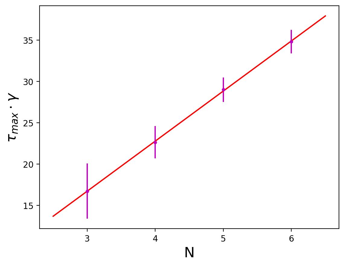
where $|c_{M}|=\max_{i}|c_{i}|$. From Eq. (16), we can find the order of magnitude for the upper bound of the mixing time, calling it as $\tau$, by definition the following relation holds: $\Delta t_{mix}\apprle\tau$. Writing $|c_{M}|=e^{\eta}$, we arrive to the expression: $\tau=\frac{N}{|\Re{\lambda_{1}}|}+\frac{\eta}{|\Re{\lambda_{1}}|}$. We have numerically computed a maximal value of $\tau$ spanning the system dimension from 3 to 6 spins. For each case, the magnetic field $h$ took the values from the set {0.01, 0.05, 0.1, 0.5, 1,5, 10}, the damping rate $\gamma$ from {0.01, 0.1, 1, 10} while the input has been fixed to be $s_{k}=0$. For all the possible combinations we have simulated 100 realizations of the Hamiltonian couplings $\{J_{i,j}\}$ and we have taken the average value of $\tau$ as a representative. In our analysis, we have selected the max average for each N, which computationally corresponds to the worst case, in order to estimate an upper bound. As shown in Fig. 5, our numerics suggest that the max order of magnitude of $\Delta t_{mix}$ scales proportionally to $\frac{N}{\gamma}$. As a result, we have numerically observed that the minimum value of $\Delta t$ required to reach the ESP, for the map of our model generated by $\bar{\mathcal{L}}(s_{k})$, scales in an efficient way with respect to the number of qubits.

References

- [1] Engineering Sciences and Medicine “Quantum Computing: Progress and Prospects” Washington, DC: The National Academies Press, 2019 DOI: 10.17226/25196
- [2] Ivan H. Deutsch “Harnessing the Power of the Second Quantum Revolution” In PRX Quantum 1 American Physical Society, 2020, pp. 020101 DOI: 10.1103/PRXQuantum.1.020101
- [3] Nicolas Gisin and Rob Thew “Quantum communication” In Nature Photonics 1.3, 2007, pp. 165–171 DOI: 10.1038/nphoton.2007.22
- [4] C. L. Degen, F. Reinhard and P. Cappellaro “Quantum sensing” In Rev. Mod. Phys. 89 American Physical Society, 2017, pp. 035002 DOI: 10.1103/RevModPhys.89.035002
- [5] S. Pirandola et al. “Advances in quantum cryptography” In Adv. Opt. Photon. 12.4 Optica Publishing Group, 2020, pp. 1012–1236 DOI: 10.1364/AOP.361502
- [6] Aram W. Harrow and Ashley Montanaro “Quantum computational supremacy” In Nature 549.7671, 2017, pp. 203–209 DOI: 10.1038/nature23458
- [7] Peter W. Shor “Polynomial-Time Algorithms for Prime Factorization and Discrete Logarithms on a Quantum Computer” In SIAM J. Comput. 26.5 USA: Society for IndustrialApplied Mathematics, 1997, pp. 1484–1509 DOI: 10.1137/S0097539795293172
- [8] Lov K Grover “A fast quantum mechanical algorithm for database search” In Proceedings of the twenty-eighth annual ACM symposium on Theory of computing, 1996, pp. 212–219 DOI: 10.1145/237814.237866
- [9] David Deutsch and Richard Jozsa “Rapid solution of problems by quantum computation” In Proceedings of the Royal Society of London. Series A: Mathematical and Physical Sciences 439.1907 The Royal Society London, 1992, pp. 553–558 DOI: 10.1098/rspa.1992.0167
- [10] Ethan Bernstein and Umesh Vazirani “Quantum complexity theory” In SIAM Journal on computing 26.5 SIAM, 1997, pp. 1411–1473 DOI: 10.1137/S0097539796300921
- [11] Yudong Cao et al. “Quantum chemistry in the age of quantum computing” In Chemical reviews 119.19 ACS Publications, 2019, pp. 10856–10915 DOI: 10.1021/acs.chemrev.8b00803
- [12] Roman Orus, Samuel Mugel and Enrique Lizaso “Quantum computing for finance: Overview and prospects” In Reviews in Physics 4 Elsevier, 2019, pp. 100028 DOI: https://doi.org/10.1016/j.revip.2019.100028
- [13] Nikitas Stamatopoulos et al. “Option pricing using quantum computers” In Quantum 4 Verein zur Förderung des Open Access Publizierens in den Quantenwissenschaften, 2020, pp. 291 DOI: https://doi.org/10.22331/q-2020-07-06-291
- [14] Jacob Biamonte et al. “Quantum machine learning” In Nature 549.7671 Nature Publishing Group, 2017, pp. 195–202 DOI: 10.1038/nature23474
- [15] John Preskill “Quantum Computing in the NISQ era and beyond” In Quantum 2 Verein zur Förderung des Open Access Publizierens in den Quantenwissenschaften, 2018, pp. 79 DOI: 10.22331/q-2018-08-06-79
- [16] Kishor Bharti et al. “Noisy intermediate-scale quantum algorithms” In Reviews of Modern Physics 94.1 APS, 2022, pp. 015004 DOI: 10.1103/RevModPhys.94.015004
- [17] Frank Verstraete, Michael M Wolf and J Ignacio Cirac “Quantum computation and quantum-state engineering driven by dissipation” In Nature physics 5.9 Nature Publishing Group, 2009, pp. 633–636 DOI: 10.1038/nphys1342
- [18] Fernando Pastawski, Lucas Clemente and Juan Ignacio Cirac “Quantum memories based on engineered dissipation” In Physical Review A 83.1 APS, 2011, pp. 012304 DOI: 10.1103/PhysRevA.83.012304
- [19] Christiane P Koch “Controlling open quantum systems: tools, achievements, and limitations” In Journal of Physics: Condensed Matter 28.21 IOP Publishing, 2016, pp. 213001 DOI: 10.1088/0953-8984/28/21/213001
- [20] Sai Vinjanampathy and Janet Anders “Quantum thermodynamics” In Contemporary Physics 57.4 Taylor & Francis, 2016, pp. 545–579 DOI: 10.1080/00107514.2016.1201896
- [21] Gonzalo Manzano and Roberta Zambrini “Quantum thermodynamics under continuous monitoring: A general framework” In AVS Quantum Science 4.2, 2022, pp. 025302 DOI: 10.1116/5.0079886
- [22] Susana F Huelga and Martin B Plenio “Vibrations, quanta and biology” In Contemporary Physics 54.4 Taylor & Francis, 2013, pp. 181–207 DOI: 10.1080/00405000.2013.829687
- [23] Gonzalo Manzano et al. “Synchronization, quantum correlations and entanglement in oscillator networks” In Scientific Reports 3.1 Nature Publishing Group, 2013, pp. 1–6 DOI: 10.1038/srep01439
- [24] Albert Cabot et al. “Unveiling noiseless clusters in complex quantum networks” In npj Quantum Information 4.1 Nature Publishing Group, 2018, pp. 1–9 DOI: 10.1038/s41534-018-0108-9
- [25] Pere Mujal et al. “Opportunities in Quantum Reservoir Computing and Extreme Learning Machines” In Advanced Quantum Technologies 4.8, 2021, pp. 1–14 DOI: 10.1002/qute.202100027
- [26] Mantas Lukoševičius, Herbert Jaeger and Benjamin Schrauwen “Reservoir computing trends” In KI-Künstliche Intelligenz 26.4 Springer, 2012, pp. 365–371 DOI: 10.1007/s13218-012-0204-5
- [27] Wolfgang Maass, Thomas Natschläger and Henry Markram “Real-Time Computing Without Stable States: A New Framework for Neural Computation Based on Perturbations” In Neural Computation 14.11, 2002, pp. 2531–2560 DOI: 10.1162/089976602760407955
- [28] Herbert Jaeger “The “echo state” approach to analysing and training recurrent neural networks-with an erratum note” In Bonn, Germany: German National Research Center for Information Technology GMD Technical Report 148.34 Bonn, 2001, pp. 13 URL: https://www.ai.rug.nl/minds/uploads/EchoStatesTechRep.pdf
- [29] Gouhei Tanaka et al. “Recent advances in physical reservoir computing: A review” In Neural Networks 115 Elsevier, 2019, pp. 100–123 DOI: https://doi.org/10.1016/j.neunet.2019.03.005
- [30] Kohei Nakajima and Ingo Fischer “Reservoir Computing” Springer, 2021 DOI: https://doi.org/10.1007/978-981-13-1687-6
- [31] John Moon et al. “Temporal data classification and forecasting using a memristor-based reservoir computing system” In Nature Electronics 2.10 Nature Publishing Group, 2019, pp. 480–487 DOI: 10.1038/s41928-019-0313-3
- [32] Julie Grollier et al. “Neuromorphic spintronics” In Nature electronics 3.7 Nature Publishing Group, 2020, pp. 360–370 DOI: 10.1038/s41928-019-0360-9
- [33] Guy Van Sande, Daniel Brunner and Miguel C. Soriano “Advances in photonic reservoir computing” In Nanophotonics 6.3, 2017, pp. 561–576 DOI: doi:10.1515/nanoph-2016-0132
- [34] Keisuke Fujii and Kohei Nakajima “Harnessing Disordered-Ensemble Quantum Dynamics for Machine Learning” In Phys. Rev. Applied 8 American Physical Society, 2017, pp. 024030 DOI: 10.1103/PhysRevApplied.8.024030
- [35] Kohei Nakajima et al. “Boosting Computational Power through Spatial Multiplexing in Quantum Reservoir Computing” In Phys. Rev. Applied 11 American Physical Society, 2019, pp. 034021 DOI: 10.1103/PhysRevApplied.11.034021
- [36] Jiayin Chen and Hendra I. Nurdin “Learning nonlinear input–output maps with dissipative quantum systems” In Quantum Information Processing 18.7 Springer ScienceBusiness Media LLC, 2019 DOI: 10.1007/s11128-019-2311-9
- [37] Quoc Hoan Tran and Kohei Nakajima “Higher-order quantum reservoir computing” In arXiv preprint arXiv:2006.08999, 2020 DOI: 10.48550/ARXIV.2006.08999
- [38] Rodrigo Martínez-Peña et al. “Information processing capacity of spin-based quantum reservoir computing systems” In Cognitive Computation Springer, 2020, pp. 1–12 DOI: 10.1007/s12559-020-09772-y
- [39] Rodrigo Araiza Bravo, Khadijeh Najafi, Xun Gao and Susanne F. Yelin “Quantum Reservoir Computing Using Arrays of Rydberg Atoms” In PRX Quantum 3 American Physical Society, 2022, pp. 030325 DOI: 10.1103/PRXQuantum.3.030325
- [40] Sanjib Ghosh, Tanjung Krisnanda, Tomasz Paterek and Timothy CH Liew “Realising and compressing quantum circuits with quantum reservoir computing” In Communications Physics 4.1 Nature Publishing Group, 2021, pp. 1–7 DOI: 10.1038/s42005-021-00606-3
- [41] Sanjib Ghosh et al. “Quantum reservoir processing” In npj Quantum Information 5 Nature Publishing Group, 2019, pp. 35 DOI: 10.1038/s41534-019-0149-8
- [42] W. D. Kalfus et al. “Hilbert space as a computational resource in reservoir computing” In Phys. Rev. Res. 4 American Physical Society, 2022, pp. 033007 DOI: 10.1103/PhysRevResearch.4.033007
- [43] Johannes Nokkala et al. “Gaussian states of continuous-variable quantum systems provide universal and versatile reservoir computing” In Communications Physics 4.1 Nature Publishing Group, 2021, pp. 1–11 DOI: 10.1038/s42005-021-00556-w
- [44] L. C. G. Govia et al. “Quantum reservoir computing with a single nonlinear oscillator” In Phys. Rev. Research 3 American Physical Society, 2021, pp. 013077 DOI: 10.1103/PhysRevResearch.3.013077
- [45] Jiayin Chen, Hendra I Nurdin and Naoki Yamamoto “Temporal information processing on noisy quantum computers” In Physical Review Applied 14.2 APS, 2020, pp. 024065 DOI: 10.1103/PhysRevApplied.14.024065
- [46] Yudai Suzuki et al. “Natural quantum reservoir computing for temporal information processing” In Scientific Reports 12.1 Nature Publishing Group, 2022, pp. 1–15 DOI: 10.1038/s41598-022-05061-w
- [47] Tomoyuki Kubota et al. “Quantum Noise-Induced Reservoir Computing” arXiv, 2022 DOI: 10.48550/ARXIV.2207.07924
- [48] Michele Spagnolo et al. “Experimental photonic quantum memristor” In Nature Photonics 16.4 Nature Publishing Group, 2022, pp. 318–323 DOI: 10.1038/s41566-022-00973-5
- [49] Joni Dambre, David Verstraeten, Benjamin Schrauwen and Serge Massar “Information processing capacity of dynamical systems” In Scientific reports 2.1 Nature Publishing Group, 2012, pp. 1–7 DOI: 10.1038/srep00514
- [50] Izzet B Yildiz, Herbert Jaeger and Stefan J Kiebel “Re-visiting the echo state property” In Neural networks 35 Elsevier, 2012, pp. 1–9 DOI: https://doi.org/10.1016/j.neunet.2012.07.005
- [51] Bruno Del Papa, Viola Priesemann and Jochen Triesch “Fading memory, plasticity, and criticality in recurrent networks” In The Functional Role of Critical Dynamics in Neural Systems Springer, 2019, pp. 95–115 DOI: 10.1007/978-3-030-20965-0_6
- [52] Sanjukta Krishnagopal, Michelle Girvan, Edward Ott and Brian R. Hunt “Separation of chaotic signals by reservoir computing” In Chaos: An Interdisciplinary Journal of Nonlinear Science 30.2, 2020, pp. 023123 DOI: 10.1063/1.5132766
- [53] Pere Mujal et al. “Analytical evidence of nonlinearity in qubits and continuous-variable quantum reservoir computing” In Journal of Physics: Complexity 2.4 IOP Publishing, 2021, pp. 045008 DOI: 10.1088/2632-072x/ac340e
- [54] M. D. SAJID ANIS et al. “Qiskit: An Open-source Framework for Quantum Computing”, 2021 DOI: 10.5281/zenodo.2573505
- [55] Marco Cattaneo et al. “Quantum simulation of dissipative collective effects on noisy quantum computers” arXiv, 2022 DOI: 10.48550/ARXIV.2201.11597
- [56] Heinz-Peter Breuer and Francesco Petruccione “The theory of open quantum systems” Oxford University Press on Demand, 2002 DOI: 10.1093/acprof:oso/9780199213900.001.0001
- [57] Goran Lindblad “On the generators of quantum dynamical semigroups” In Communications in Mathematical Physics 48.2 Springer, 1976, pp. 119–130 DOI: 10.1007/BF01608499
- [58] Vittorio Gorini, Andrzej Kossakowski and Ennackal Chandy George Sudarshan “Completely positive dynamical semigroups of N-level systems” In Journal of Mathematical Physics 17.5 American Institute of Physics, 1976, pp. 821–825 DOI: 10.1063/1.522979
- [59] Marco Cattaneo, Gian Luca Giorgi, Sabrina Maniscalco and Roberta Zambrini “Local versus global master equation with common and separate baths: superiority of the global approach in partial secular approximation” In New Journal of Physics 21.11 IOP Publishing, 2019, pp. 113045 DOI: 10.1088/1367-2630/ab54ac
- [60] Georg Fette and Julian Eggert “Short term memory and pattern matching with simple echo state networks” In International Conference on Artificial Neural Networks, 2005, pp. 13–18 Springer DOI: https://doi.org/10.1007/11550822_3
- [61] Sepp Hochreiter and Jürgen Schmidhuber “Long short-term memory” In Neural computation 9.8 MIT Press, 1997, pp. 1735–1780 DOI: 10.1007/978-3-642-24797-2_4
- [62] Gavan Lintern and Peter N Kugler “Self-organization in connectionist models: Associative memory, dissipative structures, and thermodynamic law” In Human Movement Science 10.4 Elsevier, 1991, pp. 447–483 DOI: https://doi.org/10.1016/0167-9457(91)90015-P
- [63] Rodrigo Martínez-Peña et al. “Dynamical phase transitions in quantum reservoir computing” In Physical Review Letters 127.10 APS, 2021, pp. 100502 DOI: 10.1103/PhysRevLett.127.100502
- [64] Michael C Mackey and Leon Glass “Oscillation and chaos in physiological control systems” In Science 197.4300 American Association for the Advancement of Science, 1977, pp. 287–289 DOI: 10.1126/science.267326
- [65] J Doyne Farmer and John J Sidorowich “Predicting chaotic time series” In Physical Review Letters 59.8 APS, 1987, pp. 845 DOI: 10.1103/PhysRevLett.59.845
- [66] Herbert Jaeger and Harald Haas “Harnessing nonlinearity: Predicting chaotic systems and saving energy in wireless communication” In Science 304.5667 American Association for the Advancement of Science, 2004, pp. 78–80 DOI: 10.1126/science.1091277
- [67] S Ortín et al. “A unified framework for reservoir computing and extreme learning machines based on a single time-delayed neuron” In Scientific reports 5.1 Nature Publishing Group, 2015, pp. 1–11 DOI: 10.1038/srep14945
- [68] Jaideep Pathak et al. “Using machine learning to replicate chaotic attractors and calculate Lyapunov exponents from data” In Chaos 27.12 AIP Publishing LLC, 2017, pp. 121102 DOI: 10.1063/1.5010300
- [69] Lyudmila Grigoryeva and Juan-Pablo Ortega “Echo state networks are universal” In Neural Networks 108 Elsevier, 2018, pp. 495–508 DOI: https://doi.org/10.1016/j.neunet.2018.08.025
- [70] G Manjunath “Embedding information onto a dynamical system” In Nonlinearity 35.3 IOP Publishing, 2022, pp. 1131 DOI: 10.1088/1361-6544/ac4817
- [71] Jiayin Chen “Nonlinear Convergent Dynamics for Temporal Information Processing on Novel Quantum and Classical Devices”, 2022 DOI: https://doi.org/10.26190/unsworks/24115
- [72] Davide Nigro “On the uniqueness of the steady-state solution of the Lindblad–Gorini–Kossakowski–Sudarshan equation” In Journal of Statistical Mechanics: Theory and Experiment 2019.4 IOP Publishing, 2019, pp. 043202 DOI: 10.1088/1742-5468/ab0c1c
- [73] Lyudmila Grigoryeva and Juan-Pablo Ortega “Universal Discrete-Time Reservoir Computers with Stochastic Inputs and Linear Readouts Using Non-Homogeneous State-Affine Systems” In J. Mach. Learn. Res. 19.1 JMLR.org, 2018, pp. 892–931 URL: https://dl.acm.org/doi/abs/10.5555/3291125.3291149
- [74] Inés Vega and Daniel Alonso “Dynamics of non-Markovian open quantum systems” In Rev. Mod. Phys. 89 American Physical Society, 2017, pp. 015001 DOI: 10.1103/RevModPhys.89.015001
- [75] Pere Mujal et al. “Time Series Quantum Reservoir Computing with Weak and Projective Measurements” In arXiv preprint arXiv:2205.06809, 2022 DOI: 10.48550/ARXIV.2205.06809
- [76] Jorge García-Beni, Gian Luca Giorgi, Miguel C Soriano and Roberta Zambrini “Scalable photonic platform for real-time quantum reservoir computing” In arXiv preprint arXiv:2207.14031, 2022 DOI: 10.48550/ARXIV.2207.14031
- [77] Fabrizio Minganti, Alberto Biella, Nicola Bartolo and Cristiano Ciuti “Spectral theory of Liouvillians for dissipative phase transitions” In Phys. Rev. A 98 American Physical Society, 2018, pp. 042118 DOI: 10.1103/PhysRevA.98.042118