Axions from Primordial Black Holes

Abstract

Primordial black holes (PBHs) can be significant sources of axions and axion-like particles (ALPs) in the Universe as the Hawking radiation of the PBH includes light particles when the Hawking temperature exceeds the particle’s mass. Once produced, as axions predominantly decay into photons, we may detect the enhanced photon spectrum using sensitive detectors. We introduce a new methodology by defining the time-varying decay process for particles to fly and decay over time on a cosmological scale. This paper provides the estimated photon spectrum and the flux under some simplified assumptions about PBH, 1) monochromatic mass spectrum and 2) isotropic distribution at cosmological scales. Future detectors, such as e-ASTROGAM, have great chances of detecting the signal.

I Introduction

The axion, a pseudo-Nambu-Goldstone boson associated with the spontaneously broken global Peccei-Quinn symmetry [1, 2], provides the best known solution to the strong-CP problem [3, 4]. Currently, the most attractive solutions lead to the existence of a very light axion [5, 6, 7, 8]. Axions appear in string theory [11]. An axion-like particle (ALP), a light pseudo scalar particle, may also exist, although it does not directly address the strong-CP problem. The effective Lagrangian of the axion-photon or ALP-photon interaction is given as

$$\mathcal{L}_{\text{int}}=-\frac{g_{a\gamma\gamma}}{4}aF_{\mu\nu}\tilde{F}^{\mu\nu}\,,$$ (1)

where $g_{a\gamma\gamma}=\frac{\alpha}{2\pi f_{a}}$ with the fine-structure constant $\alpha$ and the axion decay constant $f_{a}$. $a$ is the axion (or ALP), and $F_{\mu\nu}$ and $\tilde{F}^{\mu\nu}$ are the field strength tensor and its dual tensor of the photon ($A_{\mu}$), respectively.

Several astronomical sources of axion (or ALPs) have been suggested, e.g. Sun [12], supernovae [13, 14], neutron stars [15], etc., but no direct pieces of evidence are yet to be discovered [16]. We hope to see an excess in the photon signal from axion or ALPs as many astronomical observations covering a large energy region of a photon are ongoing or under consideration [17, 18, 19, 20].

Primordial black holes (PBHs) formed in the early universe through a non-stellar way [21], which can be copiously produced during inflation [22, 23] such as in realistic Higgs inflation [24, 25, 26, 27]. PBHs have been considered one of the viable candidates for dark matter (DM) [28, 29, 30] and its contribution to the fraction of DM $f_{\text{PBH}}=\Omega_{\text{PBH}}/\Omega_{\text{DM}}$ could be sizable if their masses are in a window $M_{\rm PBH}\in(10^{17},10^{23})\,{\rm g}$ [31, 32]. Once a PBH is produced, it starts to emit energy via Hawking radiation [33] with its Hawking temperature, $T_{H}\sim\frac{M_{P}^{2}}{M_{\rm PBH}}$ with the Planck mass $M_{P}\approx 2.4\times 10^{18}~{}{\rm GeV}$. Thus, PBHs can be good sources of new particles, including axions and ALPs. If the mass is small enough, the Hawking temperature exceeds the axion mass, and then the PBH can be a significant source of axions in the universe:

$$M_{\rm PBH}\lesssim\frac{M_{P}^{2}}{m_{a}}\sim\left(\frac{\rm MeV}{m_{a}}\right)\times 10^{16}\;\mathrm{g}\,.$$ (2)

The corresponding lifetime of PBH is

$$\tau_{\rm PBH}\sim 10^{4}\tau_{\rm U}\left(\frac{M_{\rm PBH}}{10^{16}\;\mathrm{g}}\right)^{3},$$ (3)

where $\tau_{\rm U}=1.38\times 10^{10}~{}{\rm yr}$ is the age of the universe.

Figure 1: A schematic picture of being considered. The curled gray line shows the photon directly released from a PBH.

Fig 1 depicts the situation we are considering in this paper. PBHs lose their energies via Hawking radiation that includes all particle species as long as their masses are small: $m\lesssim T_{H}$. As photons can propagate long without losing their energies, the precise measurement of the photons can provide information from the PBH. The photon spectrum includes the directly emitted photons from the PBH, and the photons from the decay of standard model (SM) particles and the non-SM particles such as axions and ALPs.

We organize our paper as follows. In Sec. II, we review some essential properties of PBHs and their evaporation. In Sec. III, photon fluxes from axions and ALPs emitted from PBHs are obtained by taking the elongation of the decay process over cosmological time scales. We call this effect ‘time-varying decay’. We obtain experimental bounds on ALPs and PBHs in Sec. III with the estimated photon fluxes. We conclude in Sec. V. Details on the time-varying decay are in Appendix A.

II Primordial Black Holes

There are various scenarios for the formation of PBHs [34] and these indicate that the PBH has an approximately horizontal mass when formed,

$$M_{\text{PBH}}^{\text{init}}\sim\frac{c^{3}t_{\text{form}}}{G}\sim 10^{15}\left(\frac{t_{\text{form}}}{10^{-23}\;\mathrm{s}}\right)\;\mathrm{g}\,,$$ (4)

where $M_{\text{PBH}}^{\text{init}}$ denotes the initial mass of PBHs when they formed at $t_{\text{form}}$, $c$ is the speed of light, and $G$ is the gravitational constant. According to this relation, PBHs can have a very wide mass range: if a PBH was born at Planck time $(\sim 10^{-43}\;\mathrm{s})$ $M_{\text{PBH}}\sim 10^{-5}\;\mathrm{g}$, but at $1\;\mathrm{s}$ $M_{\text{PBH}}\sim 10^{37}\;\mathrm{g}$ which is similar to the mass of a black hole that is supposed to be in the core of a galaxy. In this study, we focus on the mass range of $M_{\text{PBH}}\in(8\times 10^{14},10^{16})\;\mathrm{g}$ since the lighter ones would have already evaporated by now and the evaporation of the heavier would be too soft to be detected.

As a result of quantum effects, PBHs could evaporate emitting particles and the evaporation is related to the temperature of PBHs by the Stephan-Boltzmann radiation law, $J=\sigma T_{\text{PBH}}^{4}$ where $J$ is the radiation energy flux, $\sigma=\pi^{2}k^{4}/60\hbar^{3}c^{4}$ is the Stephan-Boltzmann constant, and $T_{\text{PBH}}$ is the temperature of PBH. The emission rate of a particle $i$ with energy $E$ from a PBH is [33]

$$\frac{\text{d}^{2}N_{i}}{\text{d}E\text{d}t}=\frac{g_{i}}{2\pi}\frac{\Gamma_{i}(E,M_{\text{PBH}})}{e^{E/k_{B}T_{\text{PBH}}}-(-1)^{2s_{i}}}\,,$$ (5)

where $g_{i}$ is the internal degrees of freedom of the emitted particle, $\Gamma_{i}$ is the greybody factor, and $s_{i}$ is the spin of the particle. In this work, the emission rate is calculated with the public code BlackHawk [35] with precisely obtained greybody factors [36, 37, 38]. We assume that PBHs have monochromatic mass $dn_{\rm{PBH}}/dM_{\rm{PBH}}=\delta(M-M_{\rm{PBH}})$, but it is rather straightforward to change with extended spectrum. We also assume isotropic distribution. For simplicity, we focus on the Schwarzschild (non-rotating and uncharged) PBHs as the angular momentum and charge emission is efficient, in general [39, 40, 41].

Figure 2: Differential fluxes of SM photons at present. The blue dot-dashed and orange dashed lines represent the photon spectrum directly emitted from PBHs and the secondary photon spectrum, respectively. The black solid line shows the combination of primary and secondary photons.

The differential photon flux by SM particles from the extragalactic PBHs is [42]

$$\dfrac{\text{d}F_{\gamma_{0}}}{\text{d}E_{\gamma_{0}}}=n_{\text{PBH}}(t_{0})\int_{t_{\text{CMB}}}^{t_{0}} \text{d}t\;(1+z(t))$$ (6)

$$\times\frac{\text{d}^{2}N_{\gamma}}{\text{d}E_{\gamma}\text{d}t}\bigg{|}_{E_{\gamma}=(1+z(t))E_{\gamma_{0}}}\,,$$

where $t_{0}$ and $t_{\text{CMB}}$ are respectively the current and CMB time, and $n_{\text{PBH}}(t_{0})=f_{\text{PBH}}\rho_{\text{DM}}/M_{\text{PBH}}$. $\gamma_{0}$ stands for the photon observed at present, and $F_{\gamma_{0}}=F_{\gamma}(t_{0})$ and $E_{\gamma_{0}}=E_{\gamma}(t_{0})$ are the flux and energy of the photon, respectively. The total flux is calculated by integrating over time after the CMB epoch implementing the redshift effect denoted by $z(t)$. Fig. 2 shows the spectra of photons from extragalactic PBHs with an initial mass of $10^{15}~{}\mathrm{g}$: the primary photons directly emitted from PBHs (blue dot-dashed), the secondary photons produced from subsequent interactions of primary SM particles (orange dashed), and the total photons (black solid). Note that due to the different spectral shapes of the primary and secondary photons, a dent feature appears around $E_{\gamma}\sim 10~{}\mathrm{MeV}$ for the total spectrum.

III Axions and ALPs from PBH

We consider just the extragalactic contribution rather than sum it with that from the galactic halo, although the extragalactic ALP flux is similar to the galactic one. In the galactic case, the strongest photon flux by the decay of ALPs from PBHs is expected from the galactic center (GC) region since PBHs is regarded densely-accumulated around the GC as the usual DM distribution. However, the SM-induced photon background is also too large around the region, leading to the weaker sensitivity of e-ASTROGAM for the GC than extragalaxies [20]. Moreover, the ALP decay to photons does not occur sufficiently in the galactic scale since ALPs are very long-lived in most of our target parameter space, as shown in Fig. 3.

Figure 3: Lifetime of ALP in the rest frame. The blue dashed line represents the age of the universe.

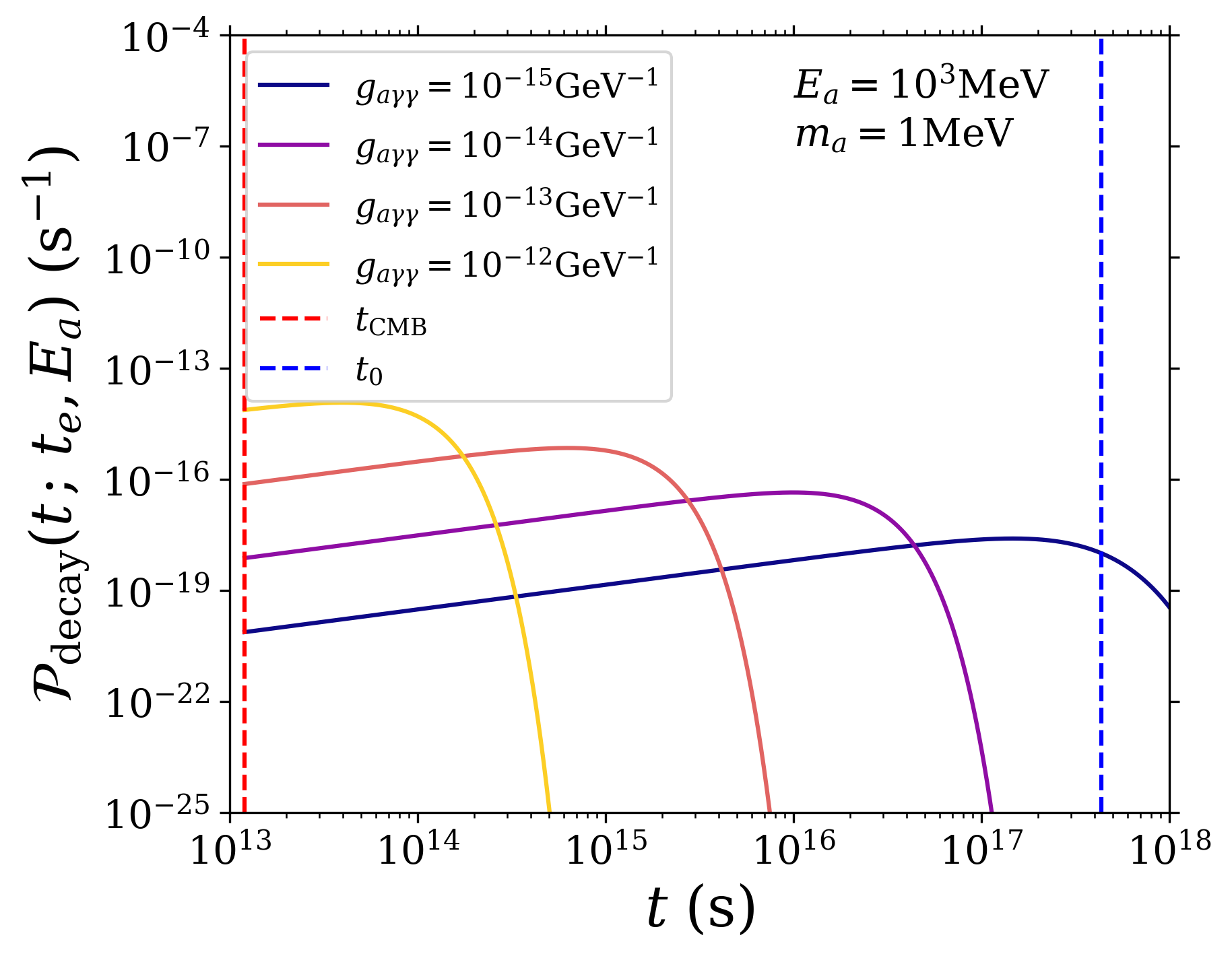
Time-varying decay of ALPs. The lifetime of a relativistic ALP is defined as a function of the total energy, mass, and coupling constant of the ALP:

$$\gamma\tau_{a}=\frac{\gamma}{\Gamma_{a\gamma\gamma}}=\frac{64\pi E_{a}}{g_{a\gamma\gamma}^{2}m_{a}^{4}}\,.$$ (7)

At a short time scale, the total energy of a particle is generally conserved, and thus the lifetime is regarded constant. On the other hand, at a long time scale, the redshift effect becomes important, and therefore the lifetime should vary with time.

Fig. 3 shows the lifetime of ALP in the rest frame, corresponding to the case of $\gamma=1$ in Eq. (7), in the parameter space which we will focus on in this study. In a fairly large parameter region, the lifetime is close to the age of the universe or even larger. In this time scale, the lifetime can no longer be constant, but When the ALP with energy $E_{a}$ at time $t_{e}$ evolves to time $t$, the redshifted energy $\mathcal{E}_{a}^{t;t_{e}}(E_{a})$ is given by

$$\mathcal{E}_{a}^{t;t_{e}}(E_{a})=\sqrt{m_{a}^{2}+\left(\frac{1+z(t)}{1+z(t_{e})}\right)^{2}(E_{a}^{2}-m_{a}^{2})}\,.$$ (8)

Since it depends on time, the Lorentz factor, decay rate, and lifetime of ALP all depend on time. Denoting the time-dependent Lorentz factor as $\gamma^{t;t_{e}}(E_{a})\equiv\mathcal{E}_{a}^{t;t_{e}}(E_{a})/m_{a}$, we have the time-dependent lifetime and decay rate,

$$\tau_{a}^{t;t_{e}}(E_{a})\equiv\gamma^{t;t_{e}}(E_{a})\tau_{a}\equiv 1/\Gamma_{a}^{t;t_{e}}(E_{a})\,.$$ (9)

Using these variables, we can precisely define the time-varying decay model, which can be found in the Appendix A. With the new decay scheme, the decay rate at time $t$ of ALPs produced from PBHs with energy $E_{a}$ at time $t_{e}$ can be calculated as

$$\phi_{a}(t;t_{e},E_{a})=\frac{\text{d}n_{a}}{\text{d}t_{e}}\cdot\mathcal{P}_{\text{decay}}(t;t_{e},E_{a})\cdot\mathcal{D}(t;t_{e})\,,$$ (10)

where $\phi_{a}(t;t_{e},E_{a})$ is the decay flux at $t$ of ALP emitted with $E_{a}$ from PBH at $t_{e}$, $\text{d}n_{a}/\text{d}t_{e}$ is the differential number density of ALP at $t_{e}$, $\mathcal{P}_{\text{decay}}(t;t_{e},E_{a})$ is the decay density function with respect to $t$ of ALP emitted with $E_{a}$ from PBH at $t_{e}$, and $\mathcal{D}(t;t_{e})=(1+z(t))^{3}/(1+z(t_{e}))^{3}$ is the dilution factor.

What we want to calculate is how much ALP will eventually decay at $t$, which can be obtained by accumulating the decay rates of all ALPs produced before $t$. Note that the energy of ALP decaying at $t$ is not $E_{a}$ but redshifted $\mathcal{E}_{a}^{t;t_{e}}(E_{a})$. If one wants to fix the energy of ALP decaying at $t$ by $\tilde{E}_{a}$, it should be converted as

$$\phi_{a}(t,\tilde{E}_{a};t_{e})=\phi_{a}(t;t_{e},E_{a})\Big{|}_{\mathcal{E}_{a}^{t;t_{e}}(E_{a})=\tilde{E}_{a}}\,.$$ (11)

Thus, we have the formula for the differential number density of ALPs decaying into photons with $E_{a}$ at $t$,

$$\frac{\text{d}n_{a}^{\text{dec}}}{\text{d}t}=\int_{t_{e}^{\text{min}}}^{t}\phi_{a}(t,E_{a};t_{e})\text{d}t_{e}\,.$$ (12)

Photons from ALP decay.

Figure 4: Photon spectrum from ALP spectrum. The blue dashed line is the spectrum of decaying ALPs, while the solid black line is the corresponding photon spectrum from the ALP decay.

Since all ALPs have their own energies, the energy spectrum of photons from ALP decay must be Lorentz-boosted. When a mother particle has an energy distribution, the distribution of decay products can be obtained using the collider-based kinematics method has been already utilized for collider physics [43, 44] and cosmic-ray signals from DM [45, 46]. We can obtain the number density of ALPs in the ALP rest frame by using BlackHawk, which is transformed to the laboratory frame. Then, we calculate the photon number density from the ALP decay using the method introduced in Refs. [43, 44, 45, 46]. In Fig. 4, the blue dashed and black solid lines are the spectrum of ALPs with $m_{a}=10~{}\mathrm{MeV}$ at $t_{\rm CMB}$ from PBHs with $m_{\rm PBH}=10^{15}~{}\mathrm{g}$ and the resulting photon spectrum, respectively. The photon spectrum shows a wider distribution toward energies lower than that of ALPs and a robust peak at $E_{\gamma}=m_{a}/2$.

Figure 5: Summary of time-varying decay of ALPs from PBH evaporation. $a$ and $\gamma$ denote axions (ALPs) and photons, respectively. The superscript ‘dec’ means decaying axions (ALPs) at that time. The information on the number density of axions (ALPs) emitted from PBH is in the red boxes. The purple boxes show how it changes in the universe and the yellow colors in the last steps show the change in the number density of photons produced from decaying axions (ALPs). The arrows drawn throughout the figure show the process by which the number density changes.

Figure 6: Differential fluxes of SM photons at present with the ALP contribution. The red dotted, orange dot-dashed, blue dashed lines denote the SM-induced photon from PBHs, the photon from prompt decay of ALPs, and the photon from time-varying decay (TV photon) of ALPs. The black solid line represents the sum of SM photons and the time-varying decay result.

When the number density of boosted photons at $t$ is $n_{\gamma}(t)$, the differential flux of photons at present from the decay of ALPs from PBHs can be obtained from Eq. (6). In Fig. 6, we compare the ALP decay contribution with the SM photon spectrum, and also with the commonly used prompt decay result. There is a region in $E_{\gamma_{0}}\sim(1-100)~{}{\rm MeV}$, where the ALP decay contribution can exceed the SM one. In addition, the time-varying decay result show a clear difference from the prompt decay.

IV Results

Figure 7: Comparison of the photons from PBHs with e-ASTROGAM sensitivity: [Top] no ALP contribution and [Bottom] with the ALP contribution. The blue dot-dashed line corresponds to the sum of the SM-induced photon flux from PBHs (red dashed) with the time-varying decay of ALPs from PBHs. The upper limit on the PBH fraction is obtained from the e-ASTROGAM sensitivity (gray solid).

We compare the photon flux from PBHs with experimental sensitivities on cosmic-ray photons by taking e-ASTROGAM [20] as our benchmark experiment, which is a future space mission of ESA. For e-ASTROGAM, $(1-2)$ orders of magnitude improved sensitivity is expected in the energy range of $\mathcal{O}(\mathrm{MeV}-\mathrm{GeV})$ compared to the existing one. Ref. [20] provides the planned galactic and extragalactic sensitivities for specific energy bins. Thus, we can find the detection prospect of e-ASTROGAM on the expected photon flux from PBHs, by integrating the differential flux obtained from Sec. III for each bin as follows,

$$I(E_{\gamma_{0}}\in(E_{n},E_{n+1}))\equiv\int_{E_{n}}^{E_{n+1}}\frac{\text{d}F_{\gamma_{0}}}{\text{d}E_{\gamma_{0}}}\text{d}E_{\gamma_{0}}\,,$$ (13)

where $\{E_{n}\}_{n=0}^{N}$ denotes a set of bins of e-ASTROGAM sensitivity. Then, we obtain the maximum value of the flux that does not exceed the sensitivity, which limits the abundance of PBH $f_{\text{PBH}}$. We apply this methodology to two cases, with and without the ALP contribution. The results for $m_{\rm PBH}=10^{15}~{}{\rm g}$ are shown in Fig. 7.

Figure 8: Deviation of limits on $f_{\rm PBH}$ with the ALP contribution. Black contours represent the improvement levels of constraints on $f_{\rm PBH}$ due to ALPs. For comparison, we show the bounds from other astronomical sources: SN1987A [14] (green) and globular clusters [47, 48] (dark green).

In Fig. 8, we show the deviation of limits with the ALP contribution from no ALP case in the ALP parameter space for two representative PBH masses, $m_{\rm PBH}=10^{15},10^{16}~{}{\rm g}$. The deviation is defined as

$$\frac{\Delta f_{\rm PBH}}{f_{{\rm PBH};\gamma}}=\frac{f_{{\rm PBH};\gamma}-f_{\rm PBH\,;\,tot}}{f_{{\rm PBH};\gamma}}\,,$$ (14)

where $f_{\rm PBH};\gamma$ and $f_{\rm PBH\,;\,tot}$ denote the PBH fraction bounds obtained by the SM photon from PBHs and the total photon with the ALP contribution, respectively. Each black contour represents the level of improvement of constraints on $f_{\rm PBH}$ due to ALPs. The improvement can be even more than $40\%$ depending on $m_{\rm PBH}$. The shaded regions corresponds to the bounds from other astronomical sources such as SN1987A [14] (green) and globular clusters [47, 48] (dark green).

Figure 9: Expected upper limits on $f_{\text{PBH}}$ for a given PBH mass when $m_{a}=1\text{MeV}$.

In Fig. 9, we present the expected upper limits on the PBH abundance for a given PBH mass in the range of ($8\times 10^{14},10^{16}$) g by fixing the ALP mass as 1 MeV. Thanks to the ALP contribution, significant improvement is possible for $m_{\rm PBH}=\mathcal{O}(10^{15}~{}{\rm g})$.

V Conclusion

Taking the quantum nature of black holes, we suggest primordial black holes (PBHs) produced in the early Universe as the source of non-standard model particles. Especially, axions and axion-like particles (ALPs) can be naturally light, and therefore they may be abundantly generated via Hawking radiation of PBHs. The produced particles have unique thermal spectra given by the Hawking temperature $T_{H}$, then induce measurable photons via their decay processes. To test this idea, in this study, we obtain the photon flux generated by the decay axions and ALPs from PBH of $M_{\rm PBH}\in(10^{14},10^{16})~{}\mathrm{g}$ mass considering the cosmological timescale of the axion decay process and the boost effects of emitted axions and ALPs. We note that the photon in $E_{\gamma}\in(1,100)\;\mathrm{MeV}$ provides distinguishable chances to see the axion effects so that e-ASTROGAM will have a great potential to detect the photons from PBH with and without axions.

Note added. During the completion of the paper, we became aware of a work [49] which also considers a similar topic.

Appendix A Time varying decay process

To obtain how many particles decay at a time with a time-varying decay rate, we should solve the decay equation. Because of the time-varying decay rate, the decay equation becomes time dependent:

$$\frac{\text{d}N_{a}}{\text{d}t}=-\Gamma_{a}^{t;t_{e}}(E_{a})N_{a}$$ (15)

$$\Rightarrow N_{a}(t;t_{e},E_{a})=N_{a}^{e}\cdot\exp\left(-\int_{t_{e}}^{t}\Gamma_{a}^{t^{\prime};t_{e}}(E_{a})\,\text{d}t^{\prime}\right),$$

where $N_{a}^{e}=N_{a}(t_{e};t_{e},E_{a})$. With a time-dependent decay rate, we can obtain a new survival probability and decay probability density function (we call it Decay density function) at time $t$ of the ALP generated from energy $E_{a}$ at time $t_{e}$ as follows:

$$P_{\text{surv}}(t;t_{e},E_{a}) = \exp\left(-\int_{t_{e}}^{t}\Gamma_{a}^{t^{\prime};t_{e}}(E_{a})\,\text{d}t^{\prime}\right),$$ (16)

$$\mathcal{P}_{\text{decay}}(t;t_{e},E_{a}) = \frac{1}{\tau_{a}^{t;t_{e}}(E_{a})}P_{\text{surv}}(t;t_{e},E_{a})\,,$$ (17)

where $P_{\text{surv}}(t;t_{e},E_{a})$ is the survival probability at time $t$ of the particle from $(t_{e},E_{a})$ and $\Gamma_{a}^{t^{\prime}:t_{e}}(E_{a})$ is the decay rate at time $t^{\prime}$ of particle from $(t_{e},E_{a})$. $\mathcal{P}_{\text{decay}}(t;t_{e},E_{a})$ is the decay density function of the particle of $(t_{e},E_{a})$ and $\tau_{a}^{t;t_{e}}(E_{a})$ is the relativistic lifetime at time $t$ of the particle from $(t_{e},E_{a})$.

In the usual exponential decay, the survival probability and the decay density function are given by

$$P_{\text{surv}}^{\text{exp}}(t;t_{e},E_{a}) = \exp\left(-\frac{\Gamma_{a}(E_{a})}{\gamma}(t-t_{e})\right),$$ (18)

$$\mathcal{P}_{\text{decay}}^{\text{exp}}(t;t_{e},E_{a}) = \frac{1}{\gamma\tau_{a}(E_{a})}P_{\text{surv}}^{\text{exp}}(t;t_{e},E_{a})\,.$$ (19)

An exponential decay with a simple linear term in the exponent and time-varying decay with integrals in the exponent clearly differ each other.

Figure 10: Decay density function: [Top] traditional exponential decay and [Bottom] time-varying decay.

As can be seen from Fig. 10, for the exponential decay the decay density function is a decreasing function. On the other hand, for time-varying decay the survival probability is almost constant ($\approx 1$) at first, but the energy decreases by the redshift effect and the lifetime also decreases accordingly, and thus the decay density function shows an increasing pattern for a considerable period of time.

Survival analysis		Time-varying decay
Term	Notation	Term	Notation
Survival function	$\displaystyle S(t)=\mathbb{P}[X>t]$	Survival probability	$P_{\text{surv}}(t;t_{e},E_{a})$
Hazard function	$\displaystyle h(t)=-\frac{\text{d}}{\text{d}t}[\log S(t)]$	Decay rate	$\Gamma_{a}^{t;t_{e}}(E_{a})$
Failure density function	$\displaystyle\int_{0}^{t}f(u)\text{d}u=1-S(t)$	Decay density function	$\displaystyle\int_{t_{e}}^{t}\mathcal{P}_{\text{decay}}(t^{\prime};t_{e},E_{a})\text{d}t^{\prime}=1-P_{\text{surv}}(t;t_{e},E_{a})$

Table 1: Comparison between survival analysis and time-varying decay

We need a well-defined decay model for the time-varying decay since it is different from the usual decay scheme. To this end, we use the survival analysis methodology [50], which is a branch of bio-statistics. In TABLE 1, we compare our notation on time-varying decay with the terms of survival analysis.

The survival function is the probability that an object will survive after time $t$. Thus, it must be a complementary cumulative distribution function (or tail function), not a probability distribution function, and for this, the following conditions must be satisfied:

• $S(0)=1$ ,

• $S(t)$ is a monotonically decreasing function.

Our survival probability $P_{\text{surv}}(t;t_{e},E_{a})$ satisfies the following conditions:

$$P_{\text{surv}}(t_{e};t_{e},E_{a})=\exp\left(-\int_{t_{e}}^{t_{e}}\Gamma_{a}^{t^{\prime};t_{e}}(E_{a})\text{ d}t^{\prime}\right)=1\,,~{}~{}~{}\quad$$ (20)

$$\frac{\text{d}\log{P_{\text{surv}}}}{\text{d}t}=-\Gamma_{a}^{t;t_{e}}(E_{a})=-\frac{1}{\tau_{a}^{t;t_{e}}(E_{a})}<0\,.$$ (21)

To count the total number of failures that occur in a specified interval, the failure rate is used in the survival analysis, which is defined by

$$\lambda(t)=\frac{S(t_{1})-S(t_{2})}{(t_{2}-t_{1})S(t_{1})}\,.$$ (22)

For infinitesimal intervals, the hazard function is defined as the limit of the failure rate,

$$h(t)=\lim_{\Delta t\to 0}\frac{S(t)-S(t+\Delta t)}{\Delta t\cdot S(t)}=-\frac{1}{S(t)}\frac{\text{d}S(t)}{\text{d}t}\,.$$ (23)

To obtain the final relation, we assume that $S(t)$ is differentiable. For our case, it corresponds to a time-varying decay rate $\Gamma_{a}^{t;t_{e}}$. Finally, to describe the continuous hazard function, the failure density function $f(t)$ is given by

$$1-S(t)=\int_{0}^{t}f(\tau)d\tau~{}\Rightarrow~{}h(t)=\frac{f(t)}{S(t)}\,.$$ (24)

In time-varying decay, it is easy to check that the decay density function satisfies the following definition:

$$\mathcal{P}_{\text{decay}}(t;t_{e},E_{a})=\Gamma_{a}^{t;t_{e}}\cdot P_{\text{surv}}(t;t_{e},E_{a})\,,$$ (25)

$$\int_{t_{e}}^{t}\mathcal{P}_{\text{decay}}(t^{\prime};t_{e},E_{a})\text{d}t^{\prime}=1-P_{\text{surv}}(t;t_{e},E_{a})\,.~{}~{}\quad$$ (26)

References

- Peccei and Quinn [1977a] R. D. Peccei and H. R. Quinn, CP Conservation in the Presence of Instantons, Phys. Rev. Lett. 38, 1440 (1977a).
- Peccei and Quinn [1977b] R. D. Peccei and H. R. Quinn, Constraints Imposed by CP Conservation in the Presence of Instantons, Phys. Rev. D 16, 1791 (1977b).
- Weinberg [1978] S. Weinberg, A New Light Boson?, Phys. Rev. Lett. 40, 223 (1978).
- Wilczek [1978] F. Wilczek, Problem of Strong and Invariance in the Presence of Instantons, Phys. Rev. Lett. 40, 279 (1978).
- Kim [1979] J. E. Kim, Weak Interaction Singlet and Strong CP Invariance, Phys. Rev. Lett. 43, 103 (1979).
- Shifman et al. [1980] M. A. Shifman, A. I. Vainshtein, and V. I. Zakharov, Can Confinement Ensure Natural CP Invariance of Strong Interactions?, Nucl. Phys. B 166, 493 (1980).
- Dine et al. [1981] M. Dine, W. Fischler, and M. Srednicki, A Simple Solution to the Strong CP Problem with a Harmless Axion, Phys. Lett. B 104, 199 (1981).
- Zhitnitsky [1980] A. R. Zhitnitsky, On Possible Suppression of the Axion Hadron Interactions. (In Russian), Sov. J. Nucl. Phys. 31, 260 (1980).
- Cheong et al. [2022a] D. Y. Cheong, K. Hamaguchi, Y. Kanazawa, S. M. Lee, N. Nagata, and S. C. Park, Axion Quality Problem and Non-Minimal Gravitational Coupling in the Palatini Formulation, (2022a), arXiv:2210.11330 [hep-th] .
- Hamaguchi et al. [2022] K. Hamaguchi, Y. Kanazawa, and N. Nagata, Axion quality problem alleviated by nonminimal coupling to gravity, Phys. Rev. D 105, 076008 (2022), arXiv:2108.13245 [hep-th] .
- Svrcek and Witten [2006] P. Svrcek and E. Witten, Axions In String Theory, JHEP 06, 051, arXiv:hep-th/0605206 .
- Di Lella and Zioutas [2002] L. Di Lella and K. Zioutas, Evidence for ubiquitous low-energy axions?, Phys. Lett. B 531, 175 (2002).
- Turner [1988] M. S. Turner, Axions from SN 1987a, Phys. Rev. Lett. 60, 1797 (1988).
- Jaeckel et al. [2018] J. Jaeckel, P. C. Malta, and J. Redondo, Decay photons from the axionlike particles burst of type II supernovae, Phys. Rev. D 98, 055032 (2018), arXiv:1702.02964 [hep-ph] .
- Morris [1986] D. E. Morris, Axion Mass Limits From Pulsar X-rays, Phys. Rev. D 34, 843 (1986).
- Choi et al. [2021] K. Choi, S. H. Im, and C. Sub Shin, Recent Progress in the Physics of Axions and Axion-Like Particles, Ann. Rev. Nucl. Part. Sci. 71, 225 (2021), arXiv:2012.05029 [hep-ph] .
- Schonfelder et al. [1993] V. Schonfelder, H. Aarts, K. Bennett, H. Deboer, J. Clear, W. Collmar, A. Connors, A. Deerenberg, R. Diehl, A. Von Dordrecht, et al., Instrument description and performance of the imaging gamma-ray telescope comptel aboard the compton gamma-ray observatory, Astrophysical Journal Supplement Series 10.1086/191794 (1993).
- Atwood et al. [2009] W. B. Atwood et al. (Fermi-LAT), The Large Area Telescope on the Fermi Gamma-ray Space Telescope Mission, Astrophys. J. 697, 1071 (2009), arXiv:0902.1089 [astro-ph.IM] .
- Abeysekara et al. [2013] A. U. Abeysekara et al., Sensitivity of the High Altitude Water Cherenkov Detector to Sources of Multi-TeV Gamma Rays, Astropart. Phys. 50-52, 26 (2013), arXiv:1306.5800 [astro-ph.HE] .
- Tavani et al. [2018] M. Tavani et al. (e-ASTROGAM), Science with e-ASTROGAM: A space mission for MeV–GeV gamma-ray astrophysics, JHEAp 19, 1 (2018), arXiv:1711.01265 [astro-ph.HE] .
- Hawking [1971] S. Hawking, Gravitationally collapsed objects of very low mass, Mon. Not. Roy. Astron. Soc. 152, 75 (1971).
- Ivanov et al. [1994] P. Ivanov, P. Naselsky, and I. Novikov, Inflation and primordial black holes as dark matter, Phys. Rev. D 50, 7173 (1994).
- Garcia-Bellido and Ruiz Morales [2017] J. Garcia-Bellido and E. Ruiz Morales, Primordial black holes from single field models of inflation, Phys. Dark Univ. 18, 47 (2017), arXiv:1702.03901 [astro-ph.CO] .
- Hamada et al. [2015] Y. Hamada, H. Kawai, K.-y. Oda, and S. C. Park, Higgs inflation from Standard Model criticality, Phys. Rev. D 91, 053008 (2015), arXiv:1408.4864 [hep-ph] .
- Hamada et al. [2014] Y. Hamada, H. Kawai, K.-y. Oda, and S. C. Park, Higgs Inflation is Still Alive after the Results from BICEP2, Phys. Rev. Lett. 112, 241301 (2014), arXiv:1403.5043 [hep-ph] .
- Cheong et al. [2021] D. Y. Cheong, S. M. Lee, and S. C. Park, Primordial black holes in Higgs- inflation as the whole of dark matter, JCAP 01, 032, arXiv:1912.12032 [hep-ph] .
- Cheong et al. [2022b] D. Y. Cheong, K. Kohri, and S. C. Park, The inflaton that could: primordial black holes and second order gravitational waves from tachyonic instability induced in Higgs-R 2 inflation, JCAP 10, 015, arXiv:2205.14813 [hep-ph] .
- Bird et al. [2016] S. Bird, I. Cholis, J. B. Muñoz, Y. Ali-Haïmoud, M. Kamionkowski, E. D. Kovetz, A. Raccanelli, and A. G. Riess, Did LIGO detect dark matter?, Phys. Rev. Lett. 116, 201301 (2016), arXiv:1603.00464 [astro-ph.CO] .
- Carr et al. [2016] B. Carr, F. Kuhnel, and M. Sandstad, Primordial Black Holes as Dark Matter, Phys. Rev. D 94, 083504 (2016), arXiv:1607.06077 [astro-ph.CO] .
- Inomata et al. [2017] K. Inomata, M. Kawasaki, K. Mukaida, Y. Tada, and T. T. Yanagida, Inflationary Primordial Black Holes as All Dark Matter, Phys. Rev. D 96, 043504 (2017), arXiv:1701.02544 [astro-ph.CO] .
- Carr et al. [2021] B. Carr, K. Kohri, Y. Sendouda, and J. Yokoyama, Constraints on primordial black holes, Rept. Prog. Phys. 84, 116902 (2021), arXiv:2002.12778 [astro-ph.CO] .
- Carr and Kuhnel [2020] B. Carr and F. Kuhnel, Primordial Black Holes as Dark Matter: Recent Developments, Ann. Rev. Nucl. Part. Sci. 70, 355 (2020), arXiv:2006.02838 [astro-ph.CO] .
- Hawking [1975] S. W. Hawking, Particle Creation by Black Holes, Commun. Math. Phys. 43, 199 (1975), [Erratum: Commun.Math.Phys. 46, 206 (1976)].
- Escrivà et al. [2022] A. Escrivà, F. Kuhnel, and Y. Tada, Primordial Black Holes, (2022), arXiv:2211.05767 [astro-ph.CO] .
- Arbey and Auffinger [2019] A. Arbey and J. Auffinger, BlackHawk: A public code for calculating the Hawking evaporation spectra of any black hole distribution, Eur. Phys. J. C 79, 693 (2019), arXiv:1905.04268 [gr-qc] .
- Ida et al. [2003] D. Ida, K.-y. Oda, and S. C. Park, Rotating black holes at future colliders: Greybody factors for brane fields, Phys. Rev. D 67, 064025 (2003), [Erratum: Phys.Rev.D 69, 049901 (2004)], arXiv:hep-th/0212108 .
- Ida et al. [2005] D. Ida, K.-y. Oda, and S. C. Park, Rotating black holes at future colliders. II. Anisotropic scalar field emission, Phys. Rev. D 71, 124039 (2005), arXiv:hep-th/0503052 .
- Ida et al. [2006] D. Ida, K.-y. Oda, and S. C. Park, Rotating black holes at future colliders. III. Determination of black hole evolution, Phys. Rev. D 73, 124022 (2006), arXiv:hep-th/0602188 .
- Page [1976a] D. N. Page, Particle Emission Rates from a Black Hole: Massless Particles from an Uncharged, Nonrotating Hole, Phys. Rev. D 13, 198 (1976a).
- Page [1976b] D. N. Page, Particle Emission Rates from a Black Hole. 2. Massless Particles from a Rotating Hole, Phys. Rev. D 14, 3260 (1976b).
- Page [1977] D. N. Page, Particle Emission Rates from a Black Hole. 3. Charged Leptons from a Nonrotating Hole, Phys. Rev. D 16, 2402 (1977).
- Carr et al. [2010] B. J. Carr, K. Kohri, Y. Sendouda, and J. Yokoyama, New cosmological constraints on primordial black holes, Phys. Rev. D 81, 104019 (2010), arXiv:0912.5297 [astro-ph.CO] .
- Agashe et al. [2013] K. Agashe, R. Franceschini, and D. Kim, Simple “invariance” of two-body decay kinematics, Phys. Rev. D 88, 057701 (2013), arXiv:1209.0772 [hep-ph] .
- Agashe et al. [2014] K. Agashe, R. Franceschini, and D. Kim, Using Energy Peaks to Measure New Particle Masses, JHEP 11, 059, arXiv:1309.4776 [hep-ph] .
- Kim and Park [2016] D. Kim and J.-C. Park, Energy peak: back to the Galactic Center GeV gamma-ray excess, Phys. Dark Univ. 11, 74 (2016), arXiv:1507.07922 [hep-ph] .
- Kim and Park [2015] D. Kim and J.-C. Park, An alternative interpretation for cosmic ray peaks, Phys. Lett. B 750, 552 (2015), arXiv:1508.06640 [hep-ph] .
- Ayala et al. [2014] A. Ayala, I. Domínguez, M. Giannotti, A. Mirizzi, and O. Straniero, Revisiting the bound on axion-photon coupling from Globular Clusters, Phys. Rev. Lett. 113, 191302 (2014), arXiv:1406.6053 [astro-ph.SR] .
- Dolan et al. [2022] M. J. Dolan, F. J. Hiskens, and R. R. Volkas, Advancing globular cluster constraints on the axion-photon coupling, JCAP 10, 096, arXiv:2207.03102 [hep-ph] .
- [49] K. Agashe, J. H. Chang, S. J. Clark, B. Dutta, Y. Tsai, and T. Xu, Detecting Axion-Like Particles with Primordial Black Holes, to appear .
- Kleinbaum and Klein [2020] D. G. Kleinbaum and M. Klein, Parametric survival models, in Survival analysis: A self-learning text (Springer, 2020) p. 289–362.