Aliasing is a Driver of Adversarial Attacks

Abstract

Aliasing is a highly important concept in signal processing, as careful consideration of resolution changes is essential in ensuring transmission and processing quality of audio, image, and video. Despite this, up until recently aliasing has received very little consideration in Deep Learning, with all common architectures carelessly sub-sampling without considering aliasing effects. In this work, we investigate the hypothesis that the existence of adversarial perturbations is due in part to aliasing in neural networks. Our ultimate goal is to increase robustness against adversarial attacks using explainable, non-trained, structural changes only, derived from aliasing first principles. Our contributions are the following. First, we establish a sufficient condition for no aliasing for general image transformations. Next, we study sources of aliasing in common neural network layers, and derive simple modifications from first principles to eliminate or reduce it. Lastly, our experimental results show a solid link between anti-aliasing and adversarial attacks. Simply reducing aliasing already results in more robust classifiers, and combining anti-aliasing with robust training out-performs solo robust training on $L_{2}$ attacks with none or minimal losses in performance on $L_{\infty}$ attacks.

1 Motivation

Deep Neural Networks (DNN) have become the state of the art in many different machine learning tasks. In particular, Deep Convolutional Networks have achieved near human-level accuracy in image classification challenges [16, 10]. However, many real-world applications require high standards of reliability, safety, and interpretability; in this sense, DNNs are not yet up to the task. One of the key reasons for this setback is the existence of adversarial examples, imperceptible perturbations to images that drastically change the predictions of neural networks with very high probability [29, 7, 10].

There has been considerable work on developing defenses against adversarial examples [29, 23, 1, 39], with Adversarial Training (AT) [7, 17, 20] standing out as the strongest current paradigm. However, there have also been significant advances towards developing more powerful methods of attack [29, 7, 22, 3, 6, 28], such that the issue is as of yet far from solved. Works characterizing adversarial examples in an analytic setting [12, 30] often do so as well-chosen but general points within a neighborhood of benign images. These type of approaches yield domain agnostic frameworks revolving around functional analysis concepts like Lipschitz continuity or estimator robustness. However, adversarial attacks are not just any kind of perturbation; they are often white-like noise that is imperceptible to humans.

Our hypothesis is that adversarial attacks work in part by exploiting the phenomenon of aliasing. Formally, aliasing is a perceptual phenomenon whereby the appearance of a signal, visual or otherwise, can change drastically after sub-sampling. See Fig. 1 for a simple but enlightening toy example. As we can see, the dirty image is indistinguishable from the original clean image by a human, and yet their outputs are completely different. The culprit for this bizarre effect is the convolution stride (green box in Fig. 1) that carelessly down-samples the input. An attacker with knowledge about it is able to construct a perturbation focused on manipulating the surviving samples (pixels at even rows and columns). The discarded samples (pixels at an odd row or column) serve as extra degrees of freedom that can be used to make the attack less noticeable and more powerful. The behavior of these analytically constructed attacks is remarkably similar to low-amplitude, gradient-driven attacks: they are imperceptible by humans and drastically change the feature maps of a network. It is thus plausible that attacks may be exploiting aliasing.

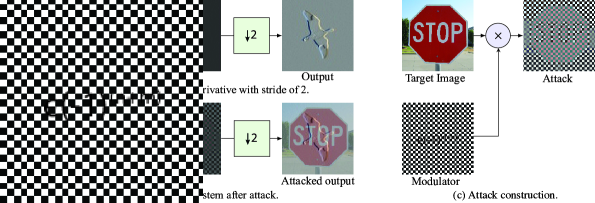
Figure 1: Analytic aliasing-based attack of a toy system that computes the horizontal image gradient, shown in (a). As this simple system has aliasing, an attacker, shown in (b), can inject a high frequency pattern to dramatically change the output with an imperceptible change to the input. The dynamic range of the images has been re-scaled to [0,1] for visualization purposes. In this example $\epsilon=\frac{16}{255}$.

2 Related work

Adversarial Attacks, broadly speaking, can be split into two types: low-amplitude and large-amplitude attacks. Low-amplitude attacks enforce imperceptibility by adding a limited $L_{p}$ constraint to the adversarial noise. Historically, the most common choice has been $p=\infty$, but there is recent work that has called this decision into question [3, 2, 6] by showing that protection against $L_{\infty}$ attacks does not imply protection against $L_{1}$ or $L_{2}$. Well known attacks of this type are FGSM ($L_{\infty}$) [7], DeepFool ($L_{2}$) [22], PGD ($L_{\infty},L_{2}$) [20], CW ($L_{2}$) [3], EAD ($L_{1}+L_{2}$) [6], and DI-FGSM ($L_{\infty}$) [37]. Large-amplitude attacks discard the $L_{p}$ constraint and instead leverage knowledge of the human visual system to produce imperceptible adversarial noises. For example, STA [33] slightly alters the shape of MNIST [19] digits in a way that fools classifiers, yet evades human detection. Another interesting work in this area involves attacking the scaling algorithms that precede most Neural Classifiers, as done in [34]. The attack is independent of the classifier architecture and requires parallel work on robust scaling algorithms to combat as in Quiring et al. [25]. The small transformations considered in [41] are also imperceptible yet radically change predictions.

Adversarial Defenses can also be split into two types: robustness-based and detection-based defenses. Robustness-based defenses aim to produce models that correctly classify adversarial examples. The current strongest paradigm for robustness-based defenses is AT [7, 17, 20]. While originally it seemed that AT had an essential trade-off between clean accuracy and robustness, recent work has produced approaches where this no longer seems to be the case [35, 24]. Detection based defenses [39] produce models that are able to differentiate between clean and attacked examples, and refuse to classify in the latter case. However, [2] and [28] have largely defeated these approaches.

For a detailed extensive review of work done in adversarial attacks and defenses see [38].

Aliasing in Deep Neural Networks has been a largely ignored topic until recent years. [41] presented the issue of aliasing in max-pool and strided convolution layers in terms of (lack of) translation invariance. [4] solved this problem entirely in devising a clever and simple trick by which they choose the phase of the sub-sampling via an energy criterion, rather than always using 0-phase, such that sub-samplings are now perfectly unit-shift invariant. [42] expanded on classic anti-aliasing blurring by introducing location and channel-dependent blurring. [11] took the matter further and treated aliasing in non-linearities, as well as enforced progressively stronger anti-aliasing w.r.t. depth. [13] brought the concept into GANs [8], and proved how aliasing was responsible for the detail coordinate-sticking effect. [9] proved the existence of aliasing in the down-sampling step of Convolutional Neural Networks (CNNs), and, most remarkably, made the acute observation that aliasing coincided with adversarial vulnerability. Similarly, [31, 40, 5] showed the relevance of Fourier analysis in robustness and adversarial attacks. [32] made an extensive study into the placement of blurring kernels and the benefits of explicit untrained anti-aliasing on generalization. [26] showed that while CNNs are capable of distinguishing oscillations and, in principle, implementing anti-aliasing blurring, this does not prevent aliasing from taking place.

To the best of our knowledge, we are the first to propose concrete anti-aliasing approaches as an untrained structural defense to white-box attacks. This is a completely different scope than in [4, 32], which focus on the clean generalization benefits of anti-aliasing. [9] also arrived at the hypothesis that aliasing is an underlying cause of adversarial vulnerability, but did not propose defenses.

We differ from previous work in a three-fold way. First, we expand on blurring-based anti-aliasing approaches like in [41, 32] by theoretically deriving the appropriate blurring strength. Second, we propose the completely novel Quantile ReLu, an anti-aliasing modification that is independent of blurring-based approaches. As we will see in the results section, combining blurring with the quantile modification yields additive robustness gains and is essential to obtain robustness. Lastly, our experiments empirically show that the anti-aliasing modifications we propose already serve as natural defenses that significantly increase robustness to any-amplitude single-step attacks and low-amplitude multi-step attacks. Moreover, combining anti-aliasing with robust training out-performs solo robust training on $L_{2}$ attacks of all amplitudes with no or minimal losses in performance on $L_{\infty}$ attacks.

3 Neural Networks without aliasing

Neural networks are full of aliasing. In this section, we briefly explain the concept of aliasing and establish a general approach to anti-aliasing arbitrary image transformations, which we then apply to the specific transformations found in CNNs. Fig. 3 shows a summary graphic of the adaptations used.

To combat aliasing, we expand on the existing blurring-based approaches such as in [41, 32, 13] by using theory to derive the exact blurring strength necessary, which coincides with the experimentally derived strength as was done in [13]. Furthermore, we also introduce the Quantile ReLu anti-aliasing modification, which is a new way of anti-aliasing independent of and synergistic with blurring-based approaches.

3.1 What is aliasing?

The concept of aliasing is intrinsically related to discrete sampling. In layman’s terms, the more ”complex” a continuous-domain signal, the finer the sampling needed to properly represent it. Using an insufficiently fine sampling results in visual artifacts that perceptually destroy the original signal; we call this phenomenon ”aliasing”.

Consider the example shown in Fig. 2: the main ”feature” of the signal, the right-to-left diagonals, is inverted by aliasing when sampling at an insufficient rate. Our hypothesis is that such visual artifacts in the processing of a Convolutional Neural Network (CNN) could be leveraged by attacks to confound networks, as motivated by Fig. 1, by providing a mechanism by which a seemingly innocuous signal may drastically change during processing.

The Shannon-Nyquist sampling theorem formalizes the concept of image complexity and provides the necessary sampling rate:

Theorem 3.1 (Shannon-Nyquist sampling theorem).

A continuous-domain 1-periodic signal $z$ is uniquely represented by a sampling with rate $s$ if and only if its Fourier Series (FS) contains no non-zero terms for frequencies greater than or equal to $s/2$ [27]. In the positive, we call the continuous-domain signal ”representable” and the sampling ”valid”. The greatest non-zero term frequency is called the band-limit of $z$.

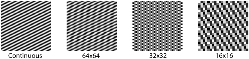
Figure 2: An insufficiently dense sampling of $\cos\left(16\pi\left(x+2y\right)\right)$ with resolution $16\times 16$ leads to disastrous aliasing, as the main feature of the signal, the bottom-left to top-right diagonals, is inverted.

We can apply the sampling theorem to derive a general approach. Given a transformation $T$ acting on discrete-domain inputs of resolution $s\times s$, we need only: (1) define $T$ for continous-domain inputs in a consisent manner, and (2) adapt $T$ such that it transforms representable continuous-domain inputs into representable continuous-domain outputs. In practical terms this will mean limiting the high-frequency information that $T$ can create, increasing the sampling rate $s$, or a combination of both.

There are three transformations in CNNs that can generate aliasing: ReLu non-linearities, sub-sampling layers, and max-pool layers. Batch-Normalizations and (unstrided) convolutional layers do not cause aliasing due to being linear and affine transformations respectively that do not change the sampling rate.

3.2 Reducing aliasing in the ReLu

It can be proven that point-wise polynomial transformations at most increase the band-limit by a factor equal to their degree. This means that up-sampling the feature map by a factor $U$ and blurring to a normalized frequency $\frac{1}{2L}$ lets us compute a polynomial non-linearity without aliasing iff $UL\geq\text{degree}$. For non-linearities that are not polynomials, but that are well-approximated by a small-degree polynomial on the distribution of the signal, we may suppress aliasing to a great degree by anti-aliasing as if we were computing the polynomial approximation. In the supp. mat., we rigorously prove that the aliasing error is bounded by twice the approximation error. Of course, what constitutes a good approximation and an acceptable aliasing error depends on the application.

In particular, the ReLu function can be approximated with less than 1% MSE on standard normal distributed inputs by the fourth degree polynomial:

$$\sum_{k=0}^{4}\langle\text{\rm{He}}_{k},\text{\rm{ReLu} }\rangle_{\mathcal{N}(0,1)}\text{\rm{He}}_{k}(t)=\frac{t}{2}-\frac{t^{4}-18t^{2}-9}{24\sqrt{2\pi}}$$ (1)

which we compute using the Hermite polynomials $\{\text{\rm{He}}_{k}\}$ and the orthogonal projection theorem. This suggests that we may compute the ReLu with a small amount of aliasing via a combination of up-sampling the feature map by a factor $U$ and blurring to a normalized frequency $\frac{1}{2L}$ for any $U,L$ with $UL\geq 4$. This theory derived conjecture coincides with the practical results obtained in [13] in a Generative Adversarial Network (GAN) setting, and we use their efficient CUDA implementation in our experiments.

Unfortunately, it appears that blurring alone is insufficient to prevent aliasing in an adversarial setting, where extreme cases are the norm rather than an oddity. Given an input with a very strong high-frequency bias, a small absolute aliasing error may be a large relative aliasing error with respect to the low-frequency un-aliased signal.

To correct this situation, we take the following complementary approach which we apply in tandem with the blurring-type modification of [13]. A ReLu non-linearity can be thought of as a non-uniform sampling that keeps positive samples and discards negative samples. Thus, we can reduce the relative aliasing error produced by enforcing a floor on the % of samples that ”survive”, as this ensures an upper bound on how much the ReLu operation can change our signal. We call this Quantile Adjustment (QA).

Definition 3.2 (Quantile Adjusted ReLu).

The Quantile Adjusted ReLu of quantile $q$ is

$$\text{QReLu}_{q}(Z)\coloneqq\max(Z+\max(-Z_{q},0),0)$$ (2)

where $Z_{q}$ is the $q$-th quantile of $Z$. In the context of a neural net the quantile is computed channel-wise.

In our experiments, we chose to take an aggressive approach and set $q=0.4$, which ensures that 60% of the signal remains unchanged (up to a fixed per-channel additive shift).

The quantile ReLu is completely different from previous anti-aliasing approaches like in [41, 42, 32]. Our results will show that combining the quantile modification with blurring-based modifications is better than both alone and is essential towards obtaining robustness. It is also different to other modifications to non-linearities like in [36], whose Smooth ReLu is used to improve AT and is used only during the backward pass. Our QReLu is devised to reduce aliasing and improve robustness as a pure structural component only, separate from AT, and is used during both the forward and backward pass.

3.3 Eliminating aliasing in sub-sampling layers

Not a true layer as it is commonly understood, but can be thought of as a component of any layer $g$ with a stride parameter $S>1$ by factorizing $g$ into a dense evaluation (stride $1$) followed by a sub-sampling

$$g_{\text{stride}=S}=g_{\text{stride}=1}*_{S}\delta$$ (3)

where $*_{S}$ denotes convolution with stride $S$, and $\delta$ is the Kronecker delta (identity element for the convolution operation in the discrete domain). The anti-alias treatment necessary is well known from the theory of signal processing and consists of blurring to a normalized frequency $\frac{1}{2S}$ prior to sub-sampling, and is independent of the prior dense operation $g$.

3.4 Eliminating aliasing in max-pooling layers

Pooling layers may introduce aliasing in one of two ways. First, the pooling operation, if it is non-linear. Second, any posterior sub-sampling due to a non-unitary stride. The solution to the second source of aliasing is covered in Sec. 3.3; its specific application to a max-pool was introduced in [41] by the name of MaxBlurPool (MBP). The first source of aliasing is tricky to deal with using the tools we have developed, as max-pooling does not have a good small-degree polynomial approximation. Hence, we turn to a heuristic argument based on non-uniform sampling principles.

We re-interpret a max-pooling operation with $\text{kernel size}=\text{stride}=K$ as a non-uniform sampling that chooses one representative for every neighborhood of size $K\times K$. In general, we have an average ”sampling rate” of $\frac{1}{K}$, so we have to blur to a normalized frequency $\frac{1}{2K}$ in order to avoid aliasing [27, 21]. Given the appropriate blurring strength, this anti-aliasing modification is equivalent to the post-filtering of [32], though they arrived to it via a different argument. Whereas their focus was on improving training dynamics with a generalization maximizing objective, ours arises from non-uniform sampling in an adversarial setting. The advantage of our argument is that the appropriate blurring strength is an intrinsic part of it.

Without up-sampling, an anti-aliased pool may be computed as such. The first blur heuristically anti-aliases the pooling operation as just explained, and the second blur anti-aliases the implicit stride (Sec. 3.3).

$$\text{AAPool}_{\text{stride}=K}=\text{Blur}_{\frac{1}{2K},\text{stride}=K}\circ\text{Pool}_{\text{stride}=1}\circ\text{Blur}_{\frac{1}{2K}}$$ (4)

By allowing up-sampling, we can relax the strength of the first blur just like with the ReLu (Sec. 3.2).

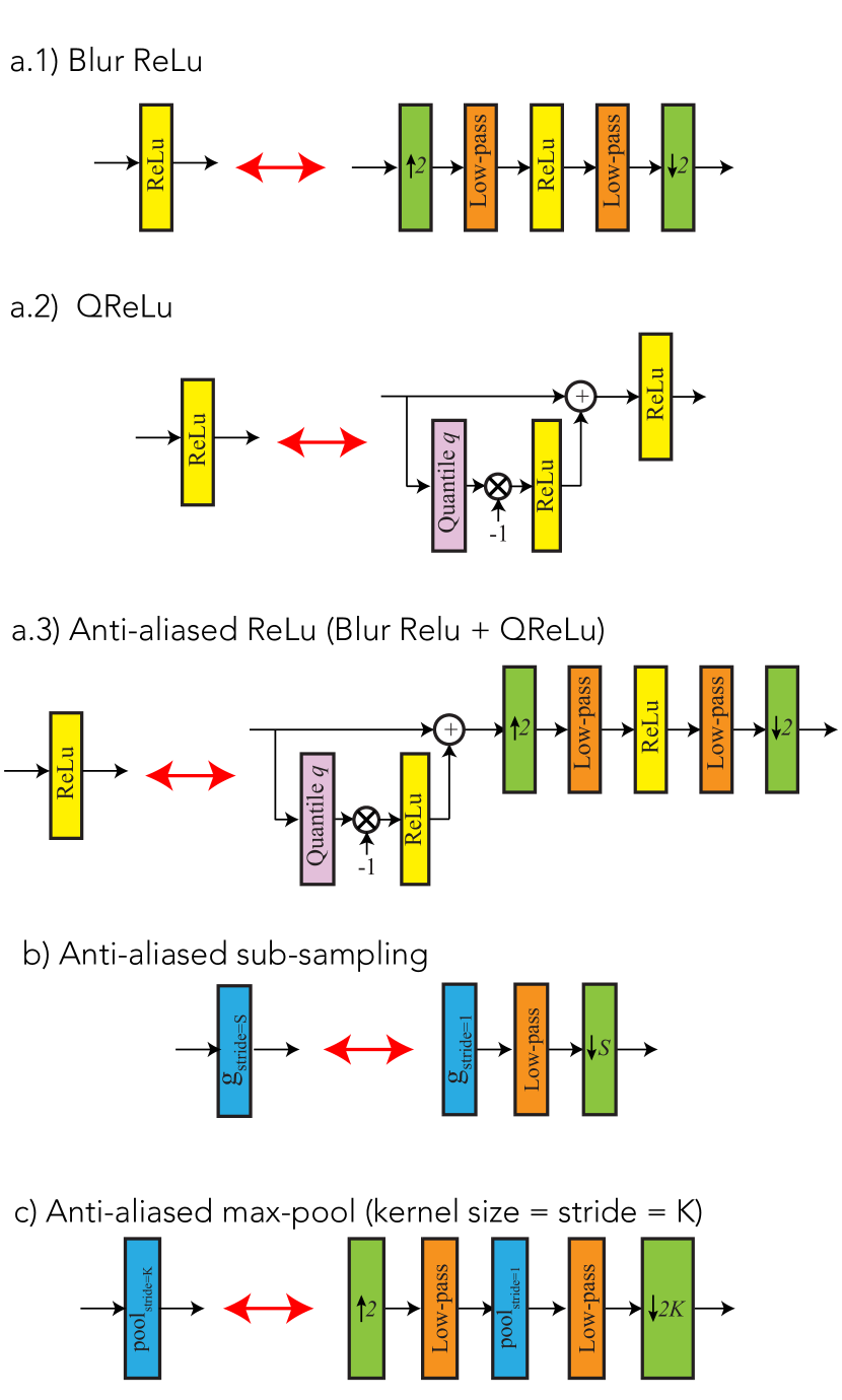
Figure 3: List of anti-aliasing replacements: (a.1) Blur ReLu , (a.2) QReLu, (a.3) Anti-aliased ReLu (combining Blur ReLu and QReLu), (b) sub-sampling, and (c) max-pooling.

3.5 Practical considerations

Practical blur kernels: In practice, reasonably sized blurring kernels have non-zero width transition bands, so there is an essential trade-off between anti-aliasing strength and quality degradation. In our experiments we have used separable Kaiser filters. As in [13], for a given target normalized frequency $\frac{1}{2L}$ we set the following Kaiser parameters: $F_{c}=\frac{1}{4L}$ to strike a balance between anti-aliasing and image quality degradation, and $F_{h}\coloneqq\frac{1}{2}-F_{c}$ to minimize rippling. Furthermore, we set $\texttt{numtaps}\coloneqq\min(\max(2\lfloor s/8\rfloor+1,3),7)$, where $s$ is the height of the feature map, to reduce boundary artifacts.

Upsampling vs blurring: In practice we may use blurring, up-sampling, or a combination of both to perform non-linear transformations without aliasing. The usage of up-sampling reduces the amount of high-frequency information that needs to be destroyed, and improves the accuracy-robustness trade-off. Any up-sampling used for this purpose has a corresponding down-sampling to keep input/output resolutions the same for each layer as seen in Fig. 3. For both the ReLu and max-pool we used an up-sampling factor of $2$, just like [13]. Moreover, up-sampling by a higher amount results in quadratic memory costs, so we think this is an acceptable compromise between compute, robustness, and accuracy.

4 Experiments and results

Previous work on anti-aliasing such as [41, 42, 32, 13] has focused on improving generalization and model quality. The sole exception is [9], which acutely observed that aliasing coincided with adversarial vulnerability, and suggested that integration of signal processing concepts into networks was necessary to correct adversarial vulnerability at the root, but left this task to future work. Our contribution is to provide exactly this integration, and propose concrete anti-aliasing modifications as an explicit un-trained structural defense to adversarial attacks. This section analyzes the effect on robustness of the modifications proposed in Sec. 3, and compares them to vanilla and AT approaches.

In particular, we observe that simply reducing aliasing already results in more robust classifiers, and combining anti-aliasing with robust training out-performs solo robust training on $L_{2}$ attacks with no or minimal losses in performance on $L_{\infty}$ attacks.

We start by detailing our experimental settings (Sec. 4.1), most notably the architectures, datasets, and adversarial attacks used for evaluation. Secondly, we investigate the workings of anti-aliasing, specifically with regards to anti-aliasing depth (Sec. 4.2) and the interplay between the blurring-based modifications and the QReLu (Sec. 4.3). Thirdly, we evaluate anti-aliasing as a defense and compare it to robust training (Sec. 4.4). Lastly, we have a discussion on computational cost (Sec. 4.5).

4.1 Experimental settings

As is standard in adversarial attacks research, we used the Cifar-10 dataset [15] for our experiments. Additionally, we also used the larger TinyImagenet dataset [18] ($64\times 64$ images as opposed to Cifar’s $32\times 32$). With respect to the architectures, we used the simple and light-weight VGG11 and the more common Resnet-50. The AT models were trained using PGD with the configuration of [20], and a half-clean half-adversarial batch approach.

We evaluate robustness using the white-box gradient attacks FGSM and PGD with varying $L_{\infty}$ and $L_{2}$ adversarial strengths (epsilon), 20 steps (for PGD), and their default [14] configurations otherwise, and consider the attacker successful if the model misclassifies the attacked input. We have elected to use white-box gradient attacks since they are the strongest attacker model, having full information about the network. Furthermore, because our anti-aliasing modifications are fully-differentiable and have the exact same behaviour in training and evaluation we eliminate concerns about gradient masking (otherwise the network would not have trained properly or at all). This means that PGD in particular is a very strongly adapted attack as it has full knowledge of our defense’s exact training gradient function, and is thus a very good candidate for benchmarking.

4.2 Is anti-aliasing at all depths required to achieve robustness?

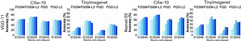
Figure 4: Defense accuracy vs number of blocks anti-aliased on the various attacks at low amplitude (epsilon=$2$). There are diminishing returns in robustness per block anti-aliased, and peak robustness is always obtained at the fourth block or earlier.

In this section, we investigate whether anti-aliasing all network layers is necessary to obtain robustness, or whether only anti-aliasing a few initial layers, where the feature map is bigger and pixel correlations are image-like, is sufficient. To this end, we split the VGG-11 and the Resnet-50 into five blocks and measure the robustness of a model with only the first $k$ blocks, $0\leq k\leq 5$, anti-aliased, which we denote by AA$(k)$ (Anti-aliasing the first $k$ blocks). $k=0$/AA(0) is equivalent to the vanilla defense i.e., doing nothing.

Fig. 4 plots accuracy vs blocks anti-aliased for low-amplitude (epsilon$=2$) attacks. Overall, we see that deeper blocks have a decreasing marginal effect, though the exact magnitudes depend on the attack and to a lower extent the model and dataset. In particular, anti-aliasing just two or three blocks yields maximum or close to maximum robustness in all but one case (Resnet-50+TinyImagenet on PGD).

Additionally, it seems that robustness plateaus faster on Cifar-10 compared to TinyImagenet, on single-step attacks compared to multi-step attacks, and on the VGG-11 compared to the Resnet-50. The first is perhaps due to the smaller sized image; at low resolutions, anti-aliasing just muddles the signal, so it makes sense that this happens earlier on Cifar-10 than TinyImagenet. The second is likely due to the relative strengths of the attack. The third might be because of the residual layer structure of the Resnet-50, which makes image dynamics last longer depth-wise in the network.

4.3 What is the interaction between the blurring and quantile approaches?

In this section, we investigate the interaction between the two anti-aliasing approaches discussed: the more standard blurring-based modifications, which we bundle together and denote by ”Blur” for simplicity, and the novel QReLu. To this end, we test defenses consisting of only one type of approach and compare them to their combination, with the vanilla defense for reference. For this experiment we anti-alias all blocks i.e., Blur+QReLu is equivalent to AA(5).

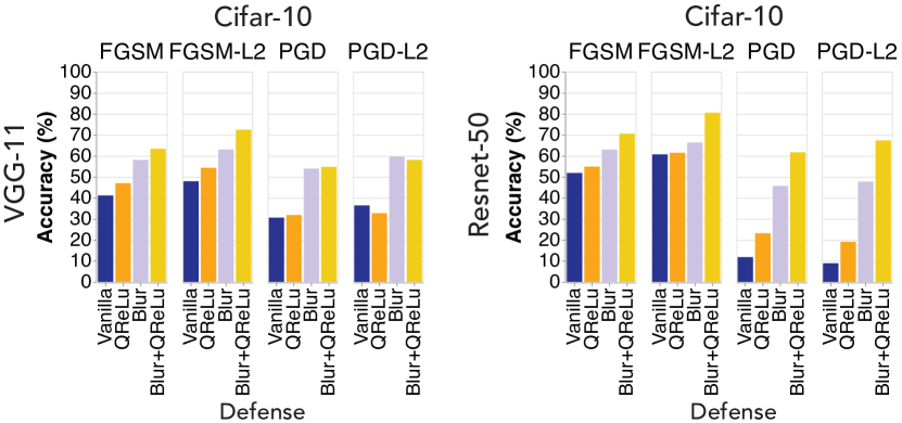
Figure 5: Defense accuracy vs type of approach on the various attacks at low amplitude (epsilon=$2$). Blur+QReLu is the combination of the blurring-based modifications and the QReLu. The two are additive or super-additive, and QReLu is especially effective on the Resnet-50.

Fig. 5 plots accuracy vs defense for low-amplitude (epsilon$=2$) attacks. We observe that Blur alone achieves similar robustness to Blur+QReLu with the VGG-11, but lags signficantly behind it on the Resnet-50. Analogously, the QReLu obtains small robustness gains alone, but is additive or super-additive when combined with Blur, especially on the Resnet-50. Blur+QReLu outperforms Blur in all but one case where it is only slightly below.

4.4 How effective is anti-aliasing as a defense?

In this section, we compare the robustness of five defenses:

• Vanilla: No defense.

• Initial Blur: Naive initial blur with [1 4 6 4 1]

• AA(5): Anti-aliasing all five blocks of the network.

• AT: Adversarial Training with PGD

• AT+AA(2): Combining adversarial training with anti-aliasing the first two blocks of the network.

Fig. 6 plots adversarial strength vs accuracy curves for the five defenses against various attacks on each architecture and dataset. The results show that, while not the full picture, aliasing plays a significant role in the vulnerability of vanilla networks to adversarial attacks.

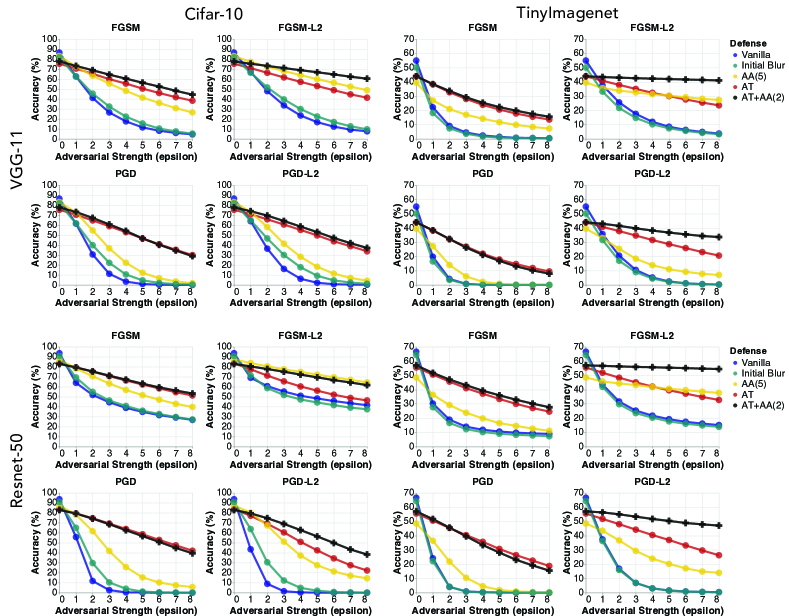
Figure 6: Defense accuracy vs adversarial strength (epsilon) curves for the Vanilla, Initial Blur, AA(5), AT, and AT+AA(2) defenses on the various attacks. Anti-aliasing by itself is already effective against low-amplitude attacks and single-step attacks, especially the $L_{2}$ variants. Combining anti-aliasing with robust training, AT+AA(2), out-performs solo robust training, AT, on $L_{2}$ attacks with only minimal losses on $L_{\infty}$ attacks.

Our simple anti-aliasing measures derived in Sec. 3 are sufficient by themselves to increase the robustness of networks significantly for low-amplitude and single-step attacks, especially for the $L_{2}$ variants. Most notably, AA(5) beats AT on the FGSM $L_{2}$ attack for all amplitudes on 3 out of the 4 dataset+architecture combinations. Moreover, the relative brittleness of Initial Blur shows that naive blurring approaches are insufficient, which further validates our methodology.

Furthermore, we observe that the AT+AA(2) defense, which combines anti-aliasing with robust training, consistently outperforms the robust training defense AT on $L_{2}$ attacks, sometimes by a very wide margin such as in Resnet-50+TinyImagenet where both $L_{2}$ attacks appear completely beaten, while maintaining statistically equal robustness on $L_{\infty}$ attacks. Adding anti-aliasing helps robust training generalize to attacks with a different norm-constraint than the one used for training. Any minimal losses in performance on $L_{\infty}$ attacks can be explained by recognizing that the robust training is done precisely with PGD, which implies the anti-aliased robust training has a smaller model search space, and additionally some overfitting to the attack might be at play given that AT is robust training with PGD $L_{\infty}$.

4.5 What is the computational cost of anti-aliasing modifications?

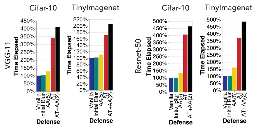
Figure 7: Training time for each defense relative to the Vanilla defense. Anti-aliasing (FA) usually results in a relatively small 10-30% increase in training time, while robust training is routinely 200-300% more costly.

In this section, we evaluate the computational cost of anti-aliasing defenses compared to robust training.

Fig. 7 plots the training time of each defense (with identical training regimes) relative to the Vanilla defense. We observe how anti-aliasing (AA(5)) usually results in a relatively small 10-30% increase in training time, with the exception of Resnet-50+TinyImagenet which had a 60% increase. Conversely, robust training routinely has a 200-300% increase in training time, with the exception of VGG-11+TinyImagenet where it had a 70% increase. Overall, robust training is routinely 2.5x-3x more expensive than anti-aliasing, which is generally fairly light-weight. The computational cost of combining anti-aliasing with robust training yields smaller metrics along a similar vein, as anti-aliasing two blocks is much cheaper than anti-aliasing five.

4.6 What are the visual effects of the defenses on the adversarial perturbations?

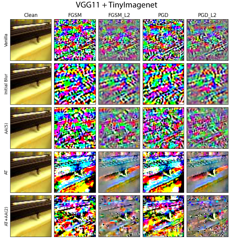
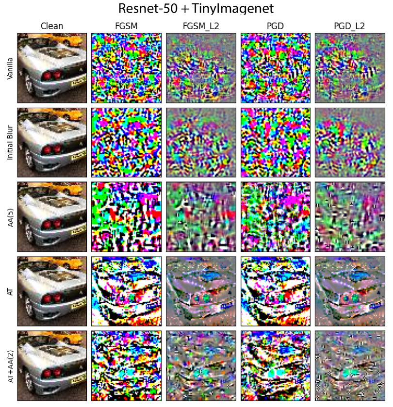
Figure 8: Perturbation examples for the different defenses and attacks at low amplitude (epsilon=$2$) on TinyImagenet. Particularly notable is the resemblance between PGD-AT noises and the clean image. A smaller degree of resemblance (particularly the edges) can be seen between FA perturbations and the clean image.

Fig. 8 showcase perturbation examples for the various defenses and attacks at low amplitude (epsilon=$2$). A natural-like attack perturbation shows that the model is more responsive to natural images and less responsive to random white-like noise, which aligns with the intuition for anti-aliasing mentioned in the introduction. Vanilla model perturbations do not resemble the clean image in either edges, coloration or texture. FA model perturbations show noticeable increase in the resemblance of the edges, but not in coloration or texture, compared to Vanilla model perturbations. PGD-AT perturbations show greatly increased resemblance in edges and texture, and slightly in coloration.

5 Conclusions

Is aliasing in neural networks responsible for their vulnerability to adversarial attacks? The experimental results presented in this paper empirically show that anti-aliasing alone makes networks significantly more robust to any-amplitude single-step attacks and low-amplitude multi-step attacks. Furthermore, combining anti-aliasing with robust training out-performs solo robust training on $L_{2}$ attacks with no or minimal losses on $L_{\infty}$ attacks.

Broader impact:

Vulnerability to attacks by current classifiers hinders their applicability to many domains. Advances in the understanding of the sources of vulnerability is important to improve classifiers and to open the door to applications where reliability is key.

Appendix A Supplementary Material

The supplementary material consists of an expanded version of Fig. 1 that includes Fourier Transforms, shedding more light on how the aliasing-based attack works, the results from Fig. 6 in tabular form, and a rigorous treatment of the claims made in Sec. 3.2.

A.1 Fourier-based analysis of aliasing-based attack

(a) Comparison of the clean and dirty input processing pipelines.

(b) Attack construction.

Figure A1: Extension of Fig. 1 including 2D Fourier Transforms (FT). We observe how the attacker, shown in (b), infiltrates the high frequency regions of the input image, shown in the corners of the FT plots. The sub-sampling operation causes high frequencies to occupy, or ”fold into”, the lower frequency space, overlapping with the clean signal and turning the attack from invisible to visible. This radical change in appearance after a sub-sampling operation is what is meant in signal processing by aliasing.

Fig. A1 is an expansion of Fig. 1 that includes Fourier Transforms (constructed to have the center position match the 2D frequency $(0,0)$). From the Fourier Transforms we observe how in the beginning, the attack lives at the edges of the frequency space, which correspond to high frequencies, and is separate from the signal living in the center, which corresponds to the lower-middle frequencies. However, after sub-sampling, the previously high frequencies start occupying the low frequency space, making the attack visible and corrupting the signal. This latter step is also known as ”frequency folding”, describing how the high frequencies ”fold into” the lower frequency space and which is an interpretation of the aliasing in the frequency domain.

Essentially, the concept of aliasing describes how an insufficient sampling rate can make high frequencies and low frequencies look the same. In this adversarial scenario, the attack, previously ”invisible” to the human eye by virtue of being a high frequency signal, becomes visible after the sub-sampling. Removing the attack via anti-aliasing prior to the sub-sampling is the only way to protect the integrity of the signal. Here we employ the domain knowledge whereby natural images are almost completely a lower-middle frequency signal, and anti-aliasing eliminates potentially dangerous content in the high-frequency space without major disruption to the clean image.

A.2 Tabular results

A.2.1 Figure 6: Defense accuracy vs adversarial strength (epsilon) curve

Attack FGSM FGSM-L2 PGD PGD-L2 Defense Epsilon Vanilla 0 86.48 86.48 86.48 86.48 2 41.10 47.91 30.58 36.37 4 17.59 23.48 3.36 6.20 8 4.57 7.66 0.03 0.28 Initial Blur 0 81.61 81.61 81.61 81.61 2 45.41 51.58 39.86 46.61 4 22.35 29.91 10.54 17.77 8 5.26 9.65 0.35 1.19 AA(5) 0 83.13 83.13 83.13 83.13 2 63.35 72.47 54.75 58.06 4 48.15 63.97 22.27 28.20 8 26.58 48.86 1.84 4.28 AT 0 75.35 75.35 75.35 75.35 2 65.30 66.29 64.67 65.80 4 55.49 57.18 52.90 55.19 8 38.34 41.32 29.90 33.74 AT+AA(2) 0 77.62 77.62 77.62 77.62 2 68.85 73.17 67.17 69.50 4 60.39 68.89 54.11 58.51 8 44.38 60.41 28.90 37.07

Table 1: Fig. 6 tabular results for VGG-11 + Cifar-10

Attack FGSM FGSM-L2 PGD PGD-L2 Defense Epsilon Vanilla 0 54.97 54.97 54.97 54.97 2 9.11 25.61 4.23 20.58 4 2.40 12.02 0.15 5.25 8 0.50 3.77 0.02 0.33 Initial Blur 0 50.15 50.15 50.15 50.15 2 7.44 21.72 3.60 16.98 4 1.70 10.25 0.09 4.52 8 0.39 3.29 0.01 0.21 AA(5) 0 39.52 39.52 39.52 39.52 2 20.94 33.87 14.01 25.37 4 14.17 31.34 2.20 13.87 8 7.31 27.35 0.09 7.06 AT 0 43.95 43.95 43.95 43.95 2 32.73 37.90 32.15 37.80 4 23.92 32.35 21.96 31.53 8 13.61 23.56 9.51 20.61 AT+AA(2) 0 43.92 43.92 43.92 43.92 2 33.64 42.98 32.21 41.47 4 25.37 42.29 21.19 38.16 8 15.55 41.03 7.92 33.62

Table 2: Tabular results for Fig. 6 for VGG-11 + TinyImagenet

Attack FGSM FGSM-L2 PGD PGD-L2 Defense Epsilon Vanilla 0 93.63 93.63 93.63 93.63 2 51.83 60.67 11.73 8.88 4 38.87 51.01 0.39 0.29 8 26.83 41.59 0.00 0.00 Initial Blur 0 90.80 90.80 90.80 90.80 2 54.93 58.68 29.66 30.49 4 40.84 47.29 3.97 4.83 8 27.19 37.49 0.03 0.11 AA(5) 0 87.44 87.44 87.44 87.44 2 70.53 80.54 61.67 67.38 4 56.85 74.91 25.71 37.23 8 39.81 64.46 5.65 14.43 AT 0 83.58 83.58 83.58 83.58 2 75.18 71.23 74.66 69.07 4 66.30 60.34 63.85 50.96 8 51.29 46.36 42.08 22.28 AT+AA(2) 0 82.95 82.95 82.95 82.95 2 75.36 77.78 74.20 74.64 4 67.15 72.20 62.63 62.73 8 53.26 61.70 39.50 38.29

Table 3: Tabular results for Fig. 6 for Resnet-50 + Cifar-10

Attack FGSM FGSM-L2 PGD PGD-L2 Defense Epsilon Vanilla 0 66.61 66.61 66.61 66.61 2 18.93 31.67 4.04 16.85 4 11.87 21.76 0.36 3.03 8 8.90 15.15 0.01 0.40 Initial Blur 0 64.33 64.33 64.33 64.33 2 16.65 29.80 4.19 16.02 4 10.21 20.33 0.23 3.05 8 7.31 13.88 0.00 0.30 AA(5) 0 48.53 48.53 48.53 48.53 2 29.19 44.36 21.83 36.67 4 19.81 41.78 4.55 23.86 8 11.13 37.74 0.34 13.96 AT 0 55.57 55.57 55.57 55.57 2 45.62 48.38 45.41 48.07 4 37.19 42.15 35.71 40.44 8 24.61 32.78 18.75 26.29 AT+AA(2) 0 57.01 57.01 57.01 57.01 2 47.07 56.30 45.62 54.98 4 39.24 55.73 33.44 51.74 8 27.66 54.43 15.48 47.10

Table 4: Tabular results for Fig. 6 for Resnet-50 + TinyImagenet

A.3 Bound on aliasing caused by arbitrary activations

Definition A.1 (Definition of a signal).

We define a signal to be a continuous, piece-wise smooth function $z:\mathbb{R}^{2}\rightarrow\mathbb{R}$ that is 1-periodic in all its arguments.

Definition A.2 (Band-limited signals).

We define the band-limit of a signal as the smallest positive integer $B$ such that the Fourier Series of the signal has coefficient $0$ for frequencies above $B$. Equivalently, signals with band-limit $B$ are those who have no (multi-dimensional) frequency content above $B$.

Proposition A.3 (Aliasing bound for point-wise functions).

Let $z$ be a signal with finite bandlimit $B$. Let $\mu(z)$ be the probability measure induced by $z$ and let $\{p_{k}\}_{k\geq 0}$ be the orthonormal polynomial family induced by $\mu(z)$. Let $\varphi:\mathbb{R}\rightarrow\mathbb{R}$ be an arbitrary point-wise function that is square-integrable with respect to $\mu(z)$. Then for any sampling rate $s>2B$, let $Z$ be the sampling of $z$ with sampling rate $s$, let $r\coloneqq\max\{k\in\mathbb{Z}:s>2kB\}$, and let $\varphi_{r}$ be the projection of $\varphi$ onto $\text{Span}\left(\{p_{k}\}_{0\leq k\leq r}\right)$.

We have that the aliasing error of the discrete computation $\varphi(Z)$ is bounded by twice the approximation error of $\varphi_{r}$

$$\left\lVert\varphi(z)-\phi_{s}(\varphi(Z)))\right\rVert^{2} =\int_{-\frac{1}{2}}^{\frac{1}{2}}\int_{-\frac{1}{2}}^{\frac{1}{2}}\left|\varphi(z)-\phi_{s}(\varphi(Z))\right|^{2}$$ (5)

$$\leq 2\left\lVert\varphi-\varphi_{r}\right\rVert^{2}_{\mu(z)}\coloneqq\int_{-\infty}^{\infty}|\varphi-\varphi_{r}|^{2}d\mu(z)$$ (6)

where $\phi_{s}$ is the ideal sinc interpolator from signal processing.

Proof.

Let $\{c_{k,l}\}_{k,l\in\mathbb{Z}}$ and $\{a_{k,l}\}_{k,l\in\mathbb{Z}}$ be the Fourier Series of $\varphi(z)$ and $\varphi_{r}(z)$ respectively. The Shannon-Nyquist Sampling Theorem [27] gives the following bound for the aliasing error in terms of the Fourier Series

$$\left\lVert\varphi(z)-\phi_{s}(\varphi(Z)\right\rVert^{2} \coloneqq\int_{-\frac{1}{2}}^{\frac{1}{2}}\int_{-\frac{1}{2}}^{\frac{1}{2}}\left|\varphi(z)-\phi_{s}(\varphi(Z))\right|^{2}$$ (7)

$$\leq 2\sum_{k,l\notin\left(-\frac{s}{2},\frac{s}{2}\right)^{2}_{\mathbb{Z}}}|c_{k,l}|^{2}$$ (8)

Since $\varphi_{r}(z)$ has band-limit $rB$ by virtue of $\varphi_{r}$ being a polynomial of degree $r$, and furthermore $s>2rB$, we have that $a_{k,l}=0$ for $k,l\notin\left(-\frac{s}{2},\frac{s}{2}\right)^{2}_{\mathbb{Z}}$ and thus

$$\sum_{k,l\notin\left(-\frac{s}{2},\frac{s}{2}\right)^{2}_{\mathbb{Z}}}|c_{k,l}|^{2}=\sum_{k,l\notin\left(-\frac{s}{2},\frac{s}{2}\right)^{2}_{\mathbb{Z}}}|c_{k,l}-a_{k,l}|^{2}\leq\sum_{k,l\in\mathbb{Z}}|c_{k,l}-a_{k,l}|^{2}$$ (9)

then, using Parseval’s Theorem and that $\varphi,\varphi_{r}$ are pointwise functions

$$\sum_{k,l\in\mathbb{Z}}|c_{k,l}-a_{k,l}|^{2} =\left\lVert\varphi(z)-\varphi_{r}(z)\right\rVert^{2}$$ (10)

$$=\int_{-\frac{1}{2}}^{\frac{1}{2}}\int_{-\frac{1}{2}}^{\frac{1}{2}}|\varphi(z)(x,y)-\varphi_{r}(z)(x,y)|^{2}dxdy$$ (11)

$$=\int_{-\frac{1}{2}}^{\frac{1}{2}}\int_{-\frac{1}{2}}^{\frac{1}{2}}|\varphi(z(x,y))-\varphi_{r}(z(x,y))|^{2}dxdy$$ (12)

which by definition of $\mu(z)$ is equal to

$$\int_{-\frac{1}{2}}^{\frac{1}{2}}\int_{-\frac{1}{2}}^{\frac{1}{2}}|\varphi(z(x,y))-\varphi_{r}(z(x,y))|^{2}dxdy =\int_{-\infty}^{\infty}|\varphi-\varphi_{r}|^{2}d\mu(z)$$ (13)

$$=\left\lVert\varphi-\varphi_{r}\right\rVert^{2}_{\mu(z)}$$ (14)

Finally, combining Eqs. 8, 9, 12 and 14 we obtain the desired result

$$\left\lVert\varphi(z)-\phi_{s}(\varphi(Z))\right\rVert^{2} \coloneqq\int_{-\frac{1}{2}}^{\frac{1}{2}}\int_{-\frac{1}{2}}^{\frac{1}{2}}\left|\varphi(z)-\phi_{s}(\varphi(Z))\right|^{2}$$ (15)

$$\leq 2\sum_{k,l\notin\left(-\frac{s}{2},\frac{s}{2}\right)^{2}_{\mathbb{Z}}}|c_{k,l}|^{2}$$ (16)

$$\leq 2\left\lVert\varphi-\varphi_{r}\right\rVert^{2}_{\mu(z)}$$ (17)

which completes the proof. ∎

Corollary A.4.

Since $\varphi$ is square-integrable with respect to $\mu(z)$, we have that

$$\lim_{s\rightarrow\infty}\left\lVert\varphi-\varphi_{r(s)}\right\rVert^{2}_{\mu_{z}}=0$$ (18)

where $r(s)\coloneqq\max\{k\in\mathbb{Z}:s>2kB\}$. Consequently, we have proven that as the sampling rate $s$ grows the aliasing error approaches zero.

Observation A.5.

Since in modern architectures Batch Normalization layers always immediately precede activation layers, we know that in most practical examples we will have $\mu(z)=\mathcal{N}(0,1)$, the standard Normal Distribution with mean $0$ and variance $1$. The orthogonal polynomial family induced by $\mathcal{N}(0,1)$ is the well-known probabilist’s Hermite polynomials. Knowing $\mu(z)$ allows us to obtain a number for the suitable sampling rate.

Corollary A.6 (Reducing aliasing in the ReLu).

We apply Proposition A.3 to the case of the ReLu.

The ReLu function $\max(z,0)$ is very well approximated (cosine similarity of $0.9907$) on $\mathcal{N}(0,1)$ by the 4-th degree polynomial

$$p(z)=\frac{z}{2}-\frac{z^{4}-18z^{2}-9}{24\sqrt{2\pi}}$$ (19)

Hence, Proposition A.3 implies a necessary sampling rate $s$ with $s>4(2B)$, where $B$ is the band-limit of the feature map pre-ReLu, to compute the ReLu with little aliasing.

References

- [1] Jacob Buckman, Aurko Roy, Colin Raffel, and Ian Goodfellow. Thermometer Encoding: One Hot Way To Resist Adversarial Examples. In International Conference on Learning Representations, 2018.
- [2] Nicholas Carlini and David A. Wagner. Adversarial examples are not easily detected: Bypassing ten detection methods. Proceedings of the 10th ACM Workshop on Artificial Intelligence and Security, 2017.
- [3] Nicholas Carlini and David A. Wagner. Towards evaluating the robustness of neural networks. 2017 IEEE Symposium on Security and Privacy (SP), pages 39–57, 2017.
- [4] Anadi Chaman and Ivan Dokmanić. Truly shift-invariant convolutional neural networks. 2021 IEEE/CVF Conference on Computer Vision and Pattern Recognition (CVPR), pages 3772–3782, 2021.
- [5] Alvin Chan, Y. Ong, and Clement Tan. How does frequency bias affect the robustness of neural image classifiers against common corruption and adversarial perturbations? In IJCAI, 2022.
- [6] Pin-Yu Chen, Yash Sharma, Huan Zhang, Jinfeng Yi, and Cho-Jui Hsieh. Ead: Elastic-net attacks to deep neural networks via adversarial examples. In AAAI, 2018.
- [7] Ian Goodfellow, Jonathon Shlens, and Christian Szegedy. Explaining and harnessing adversarial examples. In International Conference on Learning Representations, 2015.
- [8] Ian J. Goodfellow, Jean Pouget-Abadie, Mehdi Mirza, Bing Xu, David Warde-Farley, Sherjil Ozair, Aaron C. Courville, and Yoshua Bengio. Generative adversarial nets. In NIPS, 2014.
- [9] Julia Grabinski, Janis Keuper, and Margret Keuper. Aliasing coincides with CNNs vulnerability towards adversarial attacks. In The AAAI-22 Workshop on Adversarial Machine Learning and Beyond, 2022.
- [10] Kaiming He, Xiangyu Zhang, Shaoqing Ren, and Jian Sun. Deep residual learning for image recognition. In Proceedings of the IEEE Conference on Computer Vision and Pattern Recognition (CVPR), June 2016.
- [11] Md Tahmid Hossain, Shyh Wei Teng, Ferdous Sohel, and Guojun Lu. Anti-aliasing deep image classifiers using novel depth adaptive blurring and activation function. arXiv preprint arXiv:2110.00899, 2021.
- [12] Andrew Ilyas, Shibani Santurkar, Dimitris Tsipras, Logan Engstrom, Brandon Tran, and Aleksander Madry. Adversarial examples are not bugs, they are features. Advances in neural information processing systems, 32, 2019.
- [13] Tero Karras, Miika Aittala, Samuli Laine, Erik Härkönen, Janne Hellsten, Jaakko Lehtinen, and Timo Aila. Alias-Free Generative Adversarial Networks. In Proc. NeurIPS, 2021.
- [14] Hoki Kim. Torchattacks: A pytorch repository for adversarial attacks. arXiv preprint arXiv:2010.01950, 2020.
- [15] Alex Krizhevsky, Geoffrey Hinton, et al. Learning multiple layers of features from tiny images. 2009.
- [16] Alex Krizhevsky, Ilya Sutskever, and Geoffrey E. Hinton. ImageNet Classification with Deep Convolutional Neural Networks. In Proceedings of the 25th International Conference on Neural Information Processing Systems - Volume 1, NIPS’12, pages 1097–1105, Red Hook, NY, USA, 2012. Curran Associates Inc.
- [17] Alexey Kurakin, Ian J. Goodfellow, and Samy Bengio. Adversarial machine learning at scale. ArXiv, abs/1611.01236, 2017.
- [18] Le et al. Tiny ImageNet Visual Recognition Challenge.
- [19] Yann LeCun, Corinna Cortes, and Christopher J.C. Burges. The MNIST database of handwritten digits.
- [20] Aleksander Madry, Aleksandar Makelov, Ludwig Schmidt, Dimitris Tsipras, and Adrian Vladu. Towards deep learning models resistant to adversarial attacks. In International Conference on Learning Representations, 2018.
- [21] Shay Maymon and Alan V. Oppenheim. Sinc Interpolation of Nonuniform Samples. IEEE Transactions on Signal Processing, 2011.
- [22] Seyed-Mohsen Moosavi-Dezfooli, Alhussein Fawzi, and Pascal Frossard. Deepfool: A simple and accurate method to fool deep neural networks. 2016 IEEE Conference on Computer Vision and Pattern Recognition (CVPR), pages 2574–2582, 2016.
- [23] Nicolas Papernot, Patrick Mcdaniel, Xi Wu, Somesh Jha, and Ananthram Swami. Distillation as a defense to adversarial perturbations against deep neural networks. 2016 IEEE Symposium on Security and Privacy (SP), pages 582–597, 2016.
- [24] Omid Poursaeed, Tianxing Jiang, Harry Yang, Serge J. Belongie, and Ser-Nam Lim. Robustness and generalization via generative adversarial training. 2021 IEEE/CVF International Conference on Computer Vision (ICCV), pages 15691–15700, 2021.
- [25] Erwin Quiring, David Klein, Daniel Arp, Martin Johns, and Konrad Rieck. Adversarial Preprocessing: Understanding and Preventing Image-Scaling Attacks in Machine Learning. In 29th USENIX Security Symposium (USENIX Security 20), pages 1363–1380. USENIX Association, Aug. 2020.
- [26] Antônio H. Ribeiro and Thomas Schon. How convolutional neural networks deal with aliasing. ICASSP 2021 - 2021 IEEE International Conference on Acoustics, Speech and Signal Processing (ICASSP), pages 2755–2759, 2021.
- [27] Claude E. Shannon. Communication in the presence of noise. Proceedings of the IEEE, 72:1192–1201, 1984.
- [28] Yash Sharma and Pin-Yu Chen. Bypassing feature squeezing by increasing adversary strength. ArXiv, abs/1803.09868, 2018.
- [29] Christian Szegedy, Wojciech Zaremba, Ilya Sutskever, Joan Bruna, Dumitru Erhan, Ian Goodfellow, and Rob Fergus. Intriguing properties of neural networks. In 2nd International Conference on Learning Representations, ICLR 2014, 2014.
- [30] Dimitris Tsipras, Shibani Santurkar, Logan Engstrom, Alexander Turner, and Aleksander Madry. Robustness may be at odds with accuracy. arXiv preprint arXiv:1805.12152, 2018.
- [31] Yusuke Tsuzuku and Issei Sato. On the structural sensitivity of deep convolutional networks to the directions of fourier basis functions. 2019 IEEE/CVF Conference on Computer Vision and Pattern Recognition (CVPR), pages 51–60, 2019.
- [32] Cristina Vasconcelos, Hugo Larochelle, Vincent Dumoulin, Rob Romijnders, Nicolas Le Roux, and Ross Goroshin. Impact of Aliasing on Generalization in Deep Convolutional Networks. In Proceedings of the IEEE/CVF International Conference on Computer Vision (ICCV), pages 10529–10538, Oct. 2021.
- [33] Chaowei Xiao, Jun Yan Zhu, Bo Li, Warren He, Mingyan Liu, and Dawn Song. Spatially transformed adversarial examples. In 6th International Conference on Learning Representations, ICLR 2018, 2018.
- [34] Qixue Xiao, Yufei Chen, Chao Shen, Yu Chen, and Kang Li. Seeing is Not Believing: Camouflage Attacks on Image Scaling Algorithms. In 28th USENIX Security Symposium (USENIX Security 19), pages 443–460, Santa Clara, CA, Aug. 2019. USENIX Association.
- [35] Cihang Xie, Mingxing Tan, Boqing Gong, Jiang Wang, Alan L Yuille, and Quoc V Le. Adversarial examples improve image recognition. In Proceedings of the IEEE/CVF Conference on Computer Vision and Pattern Recognition, pages 819–828, 2020.
- [36] Cihang Xie, Mingxing Tan, Boqing Gong, Alan Yuille, and Quoc V Le. Smooth adversarial training. arXiv preprint arXiv:2006.14536, 2020.
- [37] Cihang Xie, Zhishuai Zhang, Yuyin Zhou, Song Bai, Jianyu Wang, Zhou Ren, and Alan L Yuille. Improving transferability of adversarial examples with input diversity. In Proceedings of the IEEE/CVF Conference on Computer Vision and Pattern Recognition, pages 2730–2739, 2019.
- [38] Han Xu, Yao Ma, Haochen Liu, Debayan Deb, Hui Liu, Jiliang Tang, and Anil K. Jain. Adversarial attacks and defenses in images, graphs and text: A review. International Journal of Automation and Computing, 17:151–178, 2020.
- [39] Weilin Xu, David Evans, and Yanjun Qi. Feature Squeezing: Detecting Adversarial Examples in Deep Neural Networks. Proceedings 2018 Network and Distributed System Security Symposium, 2018.
- [40] Dong Yin, Raphael Gontijo Lopes, Jon Shlens, Ekin Dogus Cubuk, and Justin Gilmer. A fourier perspective on model robustness in computer vision. Advances in Neural Information Processing Systems, 32, 2019.
- [41] Richard Zhang. Making Convolutional Networks Shift-Invariant Again. In ICML, 2019.
- [42] X Zou, F Xiao, Z Yu, and YJ Lee. Delving deeper into anti-aliasing in convnets. In Proceedings of the British Machine Vision Conference (BMVC), 2020, 2020.