$\text{N}^{\textbf{2}}$-SAGE: Narrow-beam Near-field SAGE Algorithm for Channel Parameter Estimation in mmWave and THz Direction-scan Measurements

Abstract

To extract channel characteristics and conduct channel modeling in millimeter-wave (mmWave) and Terahertz (THz) bands, accurate estimations of multi-path component (MPC) parameters in measured results are fundamental. However, due to high frequency and narrow antenna beams in mmWave and THz direction-scan measurements, existing channel parameter estimation algorithms are no longer effective. In this paper, a novel narrow-beam near-field space-alternating generalized expectation-maximization ($\text{N}^{\textbf{2}}$-SAGE) algorithm is proposed, which is derived by carefully considering the features of mmWave and THz direction-scan measurement campaigns, such as near field propagation, narrow antenna beams as well as asynchronous measurements in different scanning directions. The delays of MPCs are calculated using spherical wave front (SWF), which depends on delay and angles of MPCs, resulting in a high-dimensional estimation problem. To overcome this, a novel two-phase estimation process is proposed, including a rough estimation phase and an accurate estimation phase. Moreover, considering the narrow antenna beams used for mmWave and THz direction-scan measurements, the usage of partial information alleviates influence of background noises. Additionally, the phases of MPCs in different scanning directions are treated as random variables, which are estimated and reused during the estimation process, making the algorithm immune to possible phase errors. Furthermore, performance of the proposed $\text{N}^{\textbf{2}}$-SAGE algorithm is validated and compared with existing channel parameter estimation algorithms, based on simulations and measured data. Results show that the proposed $\text{N}^{\textbf{2}}$-SAGE algorithm greatly outperforms existing channel parameter estimation algorithms in terms of estimation accuracy. By using the $\text{N}^{\textbf{2}}$-SAGE algorithm, the channel is characterized more correctly and reasonably.

I Introduction

During the last several decades, the communication community has witnessed the giant leap of the communication technologies, from the first generation to the fifth generation mobile communication systems (5G). To support the large amount of intelligent devices and applications, such as metaverse, autonomous driving, etc., it is believed that the data rate in the sixth generation mobile communication system (6G) needs to exceed hundreds of gigabits per second and even Terabits per second to undertake the explosively grown data traffic [1]. As a result, the millimeter-wave (mmWave) and Terahertz (THz) bands, ranging from $0.03\text{\,}\mathrm{T}\mathrm{H}\mathrm{z}$ to $10\text{\,}\mathrm{T}\mathrm{H}\mathrm{z}$, are envisioned as a key technology to enable such high data rate [2, 3, 4]. With abundant spectrum resources and ultra-large bandwidth (more than tens of GHz), the use of mmWave and THz band can address the spectrum scarcity and capacity limitations of current wireless systems.

However, challenges remain to achieve reliable mmWave and THz communications, among which a fundamental one lies on the channel modeling in mmWave and THz bands. To thoroughly investigate propagation phenomena in mmWave and THz bands, such as significant diffuse reflections, larger diffraction loss, etc. [5, 6, 7], channel measurement campaigns are the most convincing and thus popular wave to obtain the realistic data. Generally speaking, there are mainly three kinds of methods to measure wireless channels, including omnidirectional measurements, multi-input multi-output (MIMO) measurements, and direction-scan measurements. However, due to hardware limitations in mmWave and THz bands, such as low antenna gains of omnidirectional antennas and immature antenna array techniques, THz channel measurement campaigns are mainly conducted based on the third method, which is to install directional antennas on rotators and mechanically change the pointing directions of Tx/Rx antennas to scan the spatial domain. Many research groups have utilized this method to measure mmWave and THz channels, in both indoor scenarios [8, 9, 10, 11, 12, 13, 14, 15, 16] and outdoor scenarios [17, 18, 19, 20], as thoroughly analyzed in [21].

Based on measurement results, the investigation of channel characteristics relies on accurate estimations of parameters of multi-path components (MPCs), including their time-of-arrival (ToA), direction-of-departure (DoD), direction-of-arrival (DoA), and path gains. To achieve this, high-resolution parameter estimation (HRPE) algorithms are usually used, such as space-alternating generalized expectation-maximization (SAGE) algorithm [22], RIMAX algorithm [23], etc. Among different HRPE algorithms, the SAGE algorithm is most widely-used, which has been developed and extended by many researchers during the last two decades in [24, 25, 26, 27, 28, 29]. These SAGE algorithms are mostly designed for MIMO measurements in cmWave and mmWave bands. Even though the antenna scanning patterns in direction-scan measurements can be viewed as virtual spherical arrays, there are still several facts that make these algorithms ineffective in mmWave and THz bands.

First, existing SAGE algorithms are based on the far field assumption, i.e., the array pattern is calculated assuming planer wave fronts (PWF). However, the increase of frequencies in mmWave and THz bands enlarges the Rayleigh distance, which is the boundary between near field and far field and calculated as $d=2L_{a}^{2}/\lambda$, with $L_{a}$ denoting the antenna aperture and $\lambda$ being the wavelength. For instance, for $L_{a}$ as 0.4 m and frequency as $300\text{\,}\mathrm{G}\mathrm{H}\mathrm{z}$, the Rayleigh distance is $320\text{\,}\mathrm{m}$, which is larger than measurement distances in most measurement campaigns, especially for indoor scenarios. Second, when estimating parameters of a certain MPC, traditional algorithms use channel impulse responses (CIRs) or channel transfer functions (CTFs) measured in all antenna elements. However, in direction-scan measurements, received signals of a MPC can be very weak in scanning directions that are far away from its DoD/DoA, for which the background noises could result in obvious degradation of estimation accuracy. Therefore, only partial of the measured CIRs/CTFs around the DoDs/DoAs of MPCs are helpful for the channel estimations. Third, existing SAGE algorithms omit possible phase shifts of a certain MPC on different antenna elements. However, for direction-scan measurements, since the CIRs/CTFs in different scanning directions are measured asynchronously, very accurate calibration is hard to implement and phase shifts could occur, which could greatly degrade performance of existing SAGE algorithms. In summary, if utilized in mmWave and THz direction-scan measurements, existing SAGE algorithms have low accuracy and could even produce wrong estimations. Therefore, more effective algorithms are needed to accurately estimate MPC parameters in mmWave and THz bands.

Without effective HPRE algorithms, current channel measurements in mmWave and THz bands mostly use noise elimination method to estimate MPC parameters and extract channel characteristics [10, 11, 12, 13, 14, 15, 16, 17, 18, 19, 20], i.e., the temporal samples of the CIR that are stronger than a certain path gain threshold are regarded as MPCs. However, even though the noise elimination method is easy to implement, they lack enough accuracy and fails to decouple the antenna effects in direction-scan measurement campaigns. As a result, it may produce inaccurate channel characteristics and even lead to wrong conclusions. How the coupled antenna effects in noise elimination method affects the channel characterization results needs to be carefully and thoroughly analyzed.

In this paper, we propose a novel narrow-beam near-field SAGE ($\text{N}^{2}$-SAGE) algorithm to estimate the MPC parameters in mmWave and THz bands. Furthermore, to show the efficacy of the proposed algorithm, its performance is compared with existing channel parameter estimation algorithms through simulations as well as realistic measurements. The results show that the $\text{N}^{2}$-SAGE algorithm has better estimation accuracy compared to existing channel parameter estimation methods. By using the proposed $\text{N}^{2}$-SAGE algorithm, the channel characterization in mmWave and THz bands are more accurate and reasonable. Distinctive contributions of our work are summarized as follows.

• We propose a novel $\text{N}^{2}$-SAGE algorithm, which is useful for channel parameter estimation in mmWave and THz direction-scan measurements. The high-dimensional estimation problem of delay and angles are decomposed by using a novel two-phase channel estimation process, including a rough estimation phase and an accurate estimation phase. Moreover, when estimating parameters of a certain MPC, only partial information near its DoD/DoA is used to alleviate influence of background noises. Furthermore, the phases of MPCs are modeled as scanning-direction-dependent variables, which are estimated and reused during the estimation process to avoid effects of possible phase errors.

• We compare the performance of the proposed $\text{N}^{2}$-SAGE algorithm with traditional SAGE algorithm and noise elimination method based on simulations. Influences on estimation accuracy of several factors are analyzed, such as measurement distance, noise power, etc. Results have shown that the novel designs we propose, such as two-phase estimation process, partial information utilization and direction-dependent phases of MPCs, make the proposed $\text{N}^{2}$-SAGE much more accurate compared to existing algorithms.

• We apply the proposed $\text{N}^{2}$-SAGE algorithm in real channel measurement campaigns in an indoor corridor scenario at 300 GHz. Based on the estimated MPC parameters, the power-delay-angular profile (PDAP) and channel characteristics are calculated and compared with those obtained using traditional SAGE algorithm and noise elimination method. We observe that existing estimation algorithms are less accurate and produce wrong channel characterization results, such as larger path loss, smaller K-factor, smaller azimuth spread of arrival, etc. By using the $\text{N}^{2}$-SAGE algorithm, the mmWave and THz channels can be characterized more reasonably and correctly.

The remainder of the paper is organized as follows. The $\text{N}^{2}$-SAGE algorithm is derived and explained in detail in Sec. II. Furthermore, in Sec. III, the performance of the $\text{N}^{2}$-SAGE algorithm is validated and compared with existing channel parameter estimation algorithms based on simulations. Moreover, real measured data in an indoor corridor scenario is used to compare the $\text{N}^{2}$-SAGE algorithm with existing methods in Sec. IV. Finally, Sec. V concludes the paper.

II $\text{N}^{2}$-SAGE Algorithm for Channel Parameter Estimation

To analyze the behaviours of MPCs, the parameters of MPCs, including their ToA, DoA, and DoD, need to be accurately estimated from the measurement data. In this section, we propose a novel $\text{N}^{2}$-SAGE algorithm that is dedicated for direction-scan measurement campaigns in mmWave and THz band, which is derived in detail as follows.

II-A Problem Formulation

In direction-scan measurement campaigns, both Tx and Rx are equipped with horn antennas and scan the spatial domain to receive MPCs from different directions. To cover the spatial area of interest, we assume that totally $N_{t}$ and $N_{r}$ directions are required at the Tx side and Rx side, respectively. Even though the CIRs may be measured using different kinds of equipment, such as time-domain based and frequency-domain based systems [21], the CIRs can be expressed in a general form, as derived in Appendix A. Specifically, for the $(n_{t})^{\text{th}}$ pointing direction at Tx and $(n_{r})^{\text{th}}$ pointing direction at Rx, the CIR is measured as

$$\begin{split}h_{n_{t},n_{r}}[i]=\sum_{l=1}^{L}\alpha_{l}&c_{t,n_{t}}(\bm{\Omega}_{t,l})c_{r,n_{r}}(\bm{\Omega}_{r,l})\text{e}^{j\phi_{l,n_{t},n_{r}}}\cdot\\ &R((i-1)\Delta\tau,\tau_{l,n_{t},n_{r}})+w_{n_{t},n_{r}}[i]\end{split}$$ (1)

where $\alpha_{l},\tau_{l,n_{t},n_{r}},\bm{\Omega}_{t,l},\bm{\Omega}_{r,l},\phi_{l,n_{t},n_{r}}$ denote the real-valued path gain, ToA, DoD, DoA, and phase of the $l^{\text{th}}$ MPC, respectively. The observed ToA of the $l^{\text{th}}$ MPC is dependent on the scanning directions of Tx and Rx due to variations of Tx/Rx antenna positions. Additionally, since CIRs in different scanning directions are not measured at the same time, phase shifts could occur, resulting in direction-dependent MPC phase. Moreover, $L$ is the number of MPCs. $R(x,y)$ has a similar shape with Dirac functions and is derived in Appendix A. Besides, $i$ and $\Delta\tau$ are the index and sampling interval for temporal sampling. $w_{n_{t},n_{r}}[i]$ represents the white Gaussian noise components. Furthermore, $c_{t,n_{t}}(\bm{\Omega}_{t,l})$ and $c_{r,n_{r}}(\bm{\Omega}_{r,l})$ stand for the real-valued radiation pattern of Tx and Rx horn antennas, respectively. Besides, the directions $\bm{\Omega}_{t/r,l}$ are determined by the azimuth angles $\varphi_{t/r,l}$ and elevation angles $\theta_{t/r,l}$, as

$$\bm{\Omega}_{a,l}=[\cos(\varphi_{a,l})\cos(\theta_{a,l}),\sin(\varphi_{a,l})\cos(\theta_{a,l}),\sin(\theta_{a,l})]$$ (2)

where $a$ can be either “t” or “r”, representing the DoD or DoA.

In mmWave and THz direction-scan measurements, Tx/Rx are mostly in the near-fields, for which the calculation of the observed ToA $\tau_{l,n_{t},n_{r}}$ rely on the spherical wave front (SWF). The observed ToA can be calculated by invoking the concept of virtual transmitters (receivers), as expressed as $f_{\tau}(\tau,\bm{\Omega}_{t},\bm{\Omega}_{r},n_{t},n_{r})$ in Appendix B.

By combining all discrete CIRs from all scanning directions together, we obtain

$$\begin{split}\bm{h}[i]&=\sum_{l=1}^{L}\alpha_{l}\bm{c}_{t}(\bm{\Omega}_{t,l})\bm{c}_{r}(\bm{\Omega}_{r,l})^{\text{T}}\text{e}^{j\bm{\phi}_{l}}R((i-1)\Delta\tau,\bm{\tau}_{l})+\bm{w}[i]\\ &=\sum_{l=1}^{L}\bm{s}(i;\bm{\Theta_{l}})+\bm{w}[i]\end{split}$$ (3)

where $\bm{h}$ denotes the $N_{t}\cdot N_{r}\cdot I$ CIR matrix, with $N_{t}$, $N_{r}$, $I$ denoting number of Tx scanning directions, Rx scanning directions, and temporal sampling points, respectively. Besides, $\bm{c}_{t}(\cdot)$ and $\bm{c}_{r}(\cdot)$ are column vectors that contain the radiation patterns of Tx and Rx antennas in all scanning directions, respectively. Furthermore, $\bm{\Theta}_{l}=[\bm{\tau}_{l},\bm{\Omega}_{t,l},\bm{\Omega}_{r,l},\alpha_{l},\bm{\phi}_{l}]$ contains all the parameters of the $l^{\text{th}}$ path. Moreover, $\bm{s}(i;\bm{\Theta}_{l})=\alpha_{l}\bm{c}_{t}(\bm{\Omega}_{t,l})\bm{c}_{r}(\bm{\Omega}_{r,l})^{\text{T}}\text{e}^{j\bm{\phi}_{l}}R((i-1)\Delta\tau,\bm{\tau}_{l})$ denotes the component attributed to the $l^{\text{th}}$ MPC.

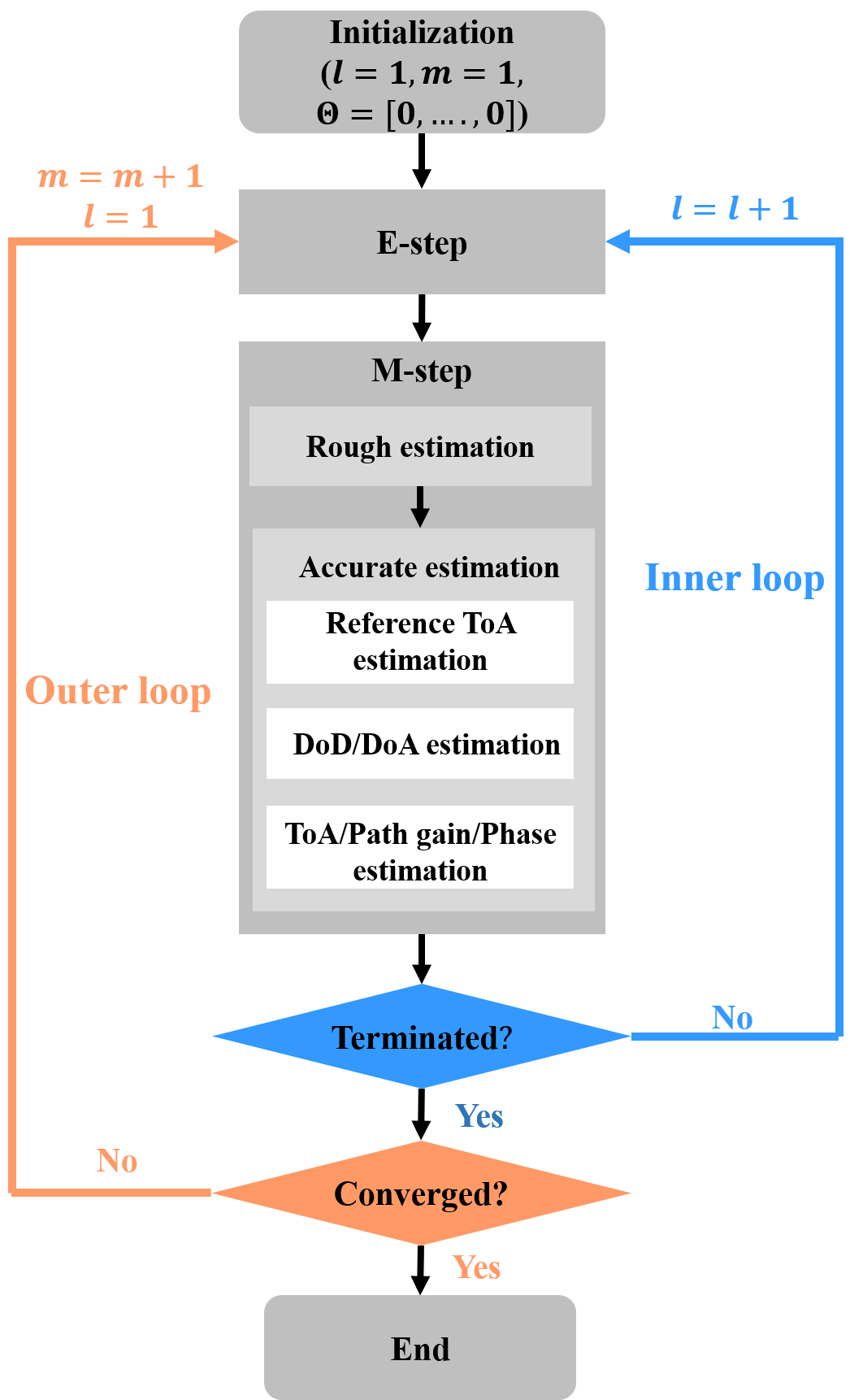
Figure 1: The flow chart of the $\text{N}^{2}$-SAGE algorithm.

Based on (3), the parameters of MPCs can be estimated iteratively by following the procedure shown in Fig. 1. The procedure includes an inner loop and an outer loop, which are elaborated as follows.

II-B Inner Loop

In each inner loop, we estimate the parameters of the significant paths, based on the following expectation (E) step and maximization (M) step.

II-B1 E-step

During the E-step, we estimate the complete data of the $l^{\text{th}}$ path by invoking parallel interference cancellation (PIC), as

$$\begin{split}\hat{\bm{x}}^{m}_{l}[i]&=\bm{h}[i]-\sum_{l^{\prime}=1}^{l-1}\bm{s}(i;\hat{\bm{\Theta}}^{m}_{l^{\prime}})-\sum_{l^{\prime}=l+1}^{L^{m-1}}\bm{s}(i;\hat{\bm{\Theta}}^{m-1}_{l^{\prime}})\\ &=\bm{s}(i;\bm{\Theta_{l}})+\sum_{l^{\prime}\neq l}^{L}\bm{E}_{l^{\prime}}^{m}+\bm{w}[i]\\ &=\bm{s}(i;\bm{\Theta_{l}})+\bm{w}^{\prime}[i]\end{split}$$ (4)

where $\hat{\bm{\Theta}}^{m}_{l^{\prime}}$ denotes the estimated values of the parameters of $(l^{\prime})^{\text{th}}$ path in the $(m)^{\text{th}}$ outer loop. Moreover, $\bm{E}_{l^{\prime}}^{m}$ and $\bm{w}[i]$ stand for residual errors due to inaccurate estimations of $(l^{\prime})^{\text{th}}$ MPC and noise effects, respectively, whose composition is treated as a whole noise term $\bm{w}^{\prime}[i]$.

II-B2 M-step

After obtaining the complete data, we then estimate the parameters of the $l^{\text{th}}$ MPC. As shown in Appendix B, for spherical wave front, the ToA difference is not only related to the DoDs/DoAs of MPCs, but also dependent on the ToAs of MPCs, i.e., the influences of ToAs, DoDs and DoAs are coupled together. Therefore, if we directly search for the accurate estimations, this is a five-dimension optimization problem since DoDs/DoAs are actually 2-D, which could consume a lot of computation and time resources. To reduce the calculation complexity, we proceed based on a two-phase estimation process, including the rough estimation phase and the accurate estimation phase.

As shown in Appendix A, the maximum of the absolute value of function $R(i;\bm{\tau}_{l})$ occurs for a certain $i$, with which $(i-1)\Delta\tau$ is very close to $\tau_{l}$. Moreover, by denoting the remaining part of $\bm{s}(i;\bm{\Theta_{l}})$ as $\bm{s}^{\prime}(\bm{\Theta_{l}})$, i.e., $\bm{s}^{\prime}(\bm{\Theta_{l}})=\alpha_{l}\bm{c}_{t}(\bm{\Omega}_{t,l})\bm{c}_{r}(\bm{\Omega}_{r,l})^{\text{T}}\text{e}^{j\bm{\phi}_{l}}$, its absolute value is maximum for scanning directions of Tx and Rx that are closest to $\bm{\Omega}_{t,l}$ and $\bm{\Omega}_{r,l}$. Therefore, assuming that the whole noise term $\bm{w}^{\prime}[i]$ is much smaller than the signal $\bm{s}(i;\bm{\Theta_{l}})$, we can make rough estimations, as

$$[i_{m},n_{t,m},n_{r,m}] =\text{arg}\max_{i,n_{t},n_{r}}([|\hat{\bm{x}}^{m}_{l}|]_{i,n_{t},n_{r}})$$ (5)

$$\hat{\tau}^{\prime}_{l} =(i_{m}-1)\Delta\tau$$ (6)

$$\hat{\bm{\Omega}}^{\prime}_{t,l} =\Omega_{\text{Tx},n_{t,m}}$$ (7)

$$\hat{\bm{\Omega}}^{\prime}_{r,l} =\Omega_{\text{Rx},n_{t,m}}$$ (8)

where $[\cdot]_{n_{1},n_{2},n_{3}}$ stands for the corresponding element of the matrix to indices $n_{1},n_{2},n_{3}$. Moreover, $i,n_{t},n_{r}$ denote the indexes of temporal sampling points, scanning angles of Tx and scanning angles of Rx, respectively. Additionally, $\Omega_{\text{Tx},n_{t,m}}$ and $\Omega_{\text{Rx},n_{t,m}}$ are $(n_{t,m})^{\text{th}}$ scanning directions of Tx and $(n_{r,m})^{\text{th}}$ scanning directions of Rx.

After obtaining the rough estimations, we then search for the accurate estimations of parameters of the $l^{\text{th}}$ MPC within the neighbourhood of the rough estimated values. We first proceed by finding the observed ToA in the $(n_{t,m})^{\text{th}}$ Tx scanning direction and $(n_{r,m})^{\text{th}}$ Rx scanning direction, as

$$\tau_{0}=\text{arg}\max_{\tau\in\bm{S}_{\tau,l}}\left|\sum_{i=1}^{I}\left[\hat{\bm{x}}^{m}_{l}\right]_{n_{t,m},n_{r,m},i}R^{*}((i-1)\Delta\tau,\tau)\right|$$ (9)

where $(\cdot)^{*}$ stands for the conjugate operation of complex numbers. Moreover, $\bm{S}_{\tau,l}$ is the local region around the rough ToA estimation, as

$$\bm{S}_{\tau,l} =\left\{\tau;\tau\in[\hat{\tau}^{\prime}_{l}-\Delta\tau,\hat{\tau}^{\prime}_{l}+\Delta\tau]\right\}$$ (10)

By treating $\tau_{0}$ as the reference ToA in the $(n_{t,m})^{\text{th}}$ Tx scanning direction and $(n_{r,m})^{\text{th}}$ Rx scanning direction, the true ToA can be calculated as a function of DoDs/DoAs of the $l^{\text{th}}$ MPC, as shown in Appendix B as $f^{-1}_{\tau}(\tau_{0},n_{t},n_{r},\bm{\Omega}_{t},\bm{\Omega}_{r})$. In this way, the ToA difference is only dependent on DoDs/DoAs. Therefore, we further find the accurate angle estimations based on the complete data, as

$$\hat{\bm{\Omega}}^{m}_{t,l} =\text{arg}\max_{\bm{\Omega}_{t}\in\bm{S}_{t,l}}z(f_{\tau}(f_{\tau}^{-1}(\tau_{0},n_{t,m},n_{r,m},\bm{\Omega}_{t},\hat{\bm{\Omega}}^{\prime}_{r,l}),$$

$$\bm{\Omega}_{t},\hat{\bm{\Omega}}^{\prime}_{r,l},\bm{N}_{t,l},n_{r,m}),\bm{\Omega}_{t},\bm{\Omega}^{\prime}_{r,l},\left[\hat{\bm{x}}_{l}^{m}\right]_{\bm{N}_{t,l},n_{r,m},1:I})$$ (11)

$$\hat{\bm{\Omega}}^{m}_{r,l} =\text{arg}\max_{\bm{\Omega}_{r}\in\bm{S}_{r,l}}z(f_{\tau}(f^{-1}_{\tau}(\tau_{0},n_{t,m},n_{r,m},\hat{\bm{\Omega}}^{\prime}_{t,l},{\bm{\Omega}}_{r}),$$

$$\hat{\bm{\Omega}}^{\prime}_{t,l},{\bm{\Omega}}_{r},n_{t,m},\bm{N}_{r,l}),\bm{\Omega}^{\prime}_{t,l},\bm{\Omega}_{r},\left[\hat{\bm{x}}_{l}^{m}\right]_{n_{t,l},\bm{N}_{r,m},1:I})$$ (12)

where the objective function $z$ to estimate directions is the maximum likelihood estimator, as [22]

$$\begin{split}z\left(\bm{\tau},\bm{\Omega}_{t},\bm{\Omega}_{r},\bm{x}\right)=2&\sum_{n_{t},n_{r},i}\mathcal{R}\left(\bm{s}^{*}\left(\bm{\tau},\bm{\Omega}_{t},\bm{\Omega}_{r},\bm{x}\right)\odot\bm{x}\right)\\ &-||\bm{s}\left(\bm{\tau},\bm{\Omega}_{t},\bm{\Omega}_{r},\bm{x}\right)||^{2}\end{split}$$ (13)

where $\bm{A}\odot\bm{B}$ represents the Hadamard product between two same-sized matrices $\bm{A}$ and $\bm{B}$. Moreover, $\bm{s}\left(\bm{\tau},\bm{\Omega}_{t},\bm{\Omega}_{r},\bm{x}\right)$ is the reconstructed signal, as

$$\bm{s}\left(\bm{\tau},\bm{\Omega}_{t},\bm{\Omega}_{r},\bm{x}\right)[i]=\alpha\bm{c}_{t}(\bm{\Omega}_{t})\bm{c}_{r}(\bm{\Omega}_{r})^{\text{T}}\text{e}^{j\bm{\phi}}\odot R((i-1)\Delta\tau,\bm{\tau})$$ (14)

where $\alpha$ and $\bm{\phi}$ are determined as

$$\alpha =\frac{\left|\sum_{n_{t},n_{r},i}\left[\bm{x}\right]_{n_{t},n_{r},i}R^{*}((i-1)\Delta\tau,\left[\bm{\tau}\right]_{n_{t},n_{r}})\right|}{\sum_{n_{t},n_{r}}c_{t,n_{t}}(\bm{\Omega}_{t})c_{r,n_{r}}(\bm{\Omega}_{r})P_{R,n_{t},n_{r}}}$$ (15)

$$\bm{\phi} =\mathscr{A}\left(\sum_{i}\bm{x}[i]\odot R^{*}((i-1)\Delta\tau,\bm{\tau})\right)$$ (16)

with

$$P_{R,n_{t},n_{r}}=\sum_{i}\left|R((i-1)\Delta\tau,\left[\bm{\tau}\right]_{n_{t},n_{r}}\right|^{2}$$ (17)

where $\mathscr{A}(\cdot)$ is the function that calculates the phase of the complex number.

Besides, $\bm{S}_{t,l},\bm{S}_{r,l},\bm{N}_{t,l},\bm{N}_{r,l}$ in (II-B2)-(II-B2) are the local regions around the rough estimations $\hat{\bm{\Omega}}^{\prime}_{t,l}$ and $\hat{\bm{\Omega}}^{\prime}_{r,l}$, which are expressed as

$$\bm{S}_{t,l} =\left\{\bm{\Omega}_{t};\left|\bm{\Omega}_{t}-\hat{\bm{\Omega}}^{\prime}_{t,l}\right|<a_{t}\right\}$$ (18)

$$\bm{S}_{r,l} =\left\{\bm{\Omega}_{r};\left|\bm{\Omega}_{r}-\hat{\bm{\Omega}}^{\prime}_{r,l}\right|<a_{r}\right\}$$ (19)

$$\bm{N}_{t,l} =\left\{n_{t};\left|\bm{\Omega}_{\text{Tx},n_{t}}-\hat{\bm{\Omega}}^{\prime}_{t,l}\right|<b_{t}\right\}$$ (20)

$$\bm{N}_{r,l} =\left\{n_{r};\left|\bm{\Omega}_{\text{Rx},n_{t}}-\hat{\bm{\Omega}}^{\prime}_{r,l}\right|<b_{r}\right\}$$ (21)

where the thresholds $a_{t/r}$ and $b_{t/r}$ are dependent on the scanning steps and beamwidths of Tx/Rx antennas. Generally speaking, $a_{t,r}$ should be large enough to at least cover half of the scanning steps of Tx/Rx and $b_{t/r}$ are set appropriately to include most of the main beam of antennas.

In (II-B2) and (II-B2), it can be observed that when estimating the DoDs of MPCs, only the CIRs in the $(n_{r,m})^{\text{th}}$ Rx scanning direction is used, since the influence of the $l^{\text{th}}$ MPC is most significant in this direction. Similarly, when estimating the DoAs of MPCs, only the CIRs in the $(n_{t,m})^{\text{th}}$ Tx scanning direction is used. Therefore, the original estimation problem of ToAs, DoDs, DoAs, which is five dimensional, is decomposed into three sub-problems in (9), (II-B2) and (II-B2) with dimensions of 1, 2, 2, which greatly reduces the time and computation resource consumption.

With the accurate estimations of DoD/DoA of the $l^{\text{th}}$ MPC, the accurate path gain, phase and ToA can be obtained as

$$\hat{\tau}^{m}_{l} =f^{-1}_{\tau}(\tau_{0},n_{t,m},n_{r,m},\hat{\bm{\Omega}}^{m}_{t,l},\hat{\bm{\Omega}}^{m}_{r,l})$$ (22)

$$\hat{\alpha}^{m}_{l} =\frac{\left|\sum_{n_{t}\in\bm{N}_{t,l},n_{r}\in\bm{N}_{r,l}}\alpha_{n_{t},n_{r}}\right|}{\sum_{n_{t}\in\bm{N}_{t,l},n_{r}\in\bm{N}_{r,l}}c_{t,n_{t}}(\hat{\bm{\Omega}}^{m}_{t,l})c_{r,n_{r}}(\hat{\bm{\Omega}}^{m}_{r,l})P_{R,n_{t},n_{r}}}$$ (23)

$$\hat{\bm{\phi}}^{m}_{l} =\mathscr{A}(\sum_{i}\hat{\bm{x}}^{m}_{l}[i]\odot R\left((i-1)\Delta\tau,\tau_{n_{t},n_{r}}\right))$$ (24)

where $\bm{N}_{t}$ and $\bm{N}_{r}$ are vectors containing all indices of Tx and Rx scanning directions, respectively. Moreover, $\alpha_{n_{t},n_{r}}$, $P_{R,n_{t},n_{r}}$, $\tau_{n_{t},n_{r}}$ are calculated as

$$\alpha_{n_{t},n_{r}} =\sum_{i=1}^{I}\left[\hat{\bm{x}}^{m}_{l}\right]_{n_{t},n_{r},i}R^{*}((i-1)\Delta\tau,\tau_{n_{t},n_{r}})$$ (25)

$$P_{R,n_{t},n_{r}} =\sum_{i=1}^{I}\left|R((i-1)\Delta\tau,\tau_{n_{t},n_{r}})\right|^{2}$$ (26)

$$\tau_{n_{t},n_{r}} =f_{\tau}(\hat{\tau}^{m}_{l},\hat{\bm{\Omega}}^{m}_{t,l},\hat{\bm{\Omega}}^{m}_{r,l},n_{t},n_{r})$$ (27)

During each inner loop, the MPCs are estimated in the descending order in light of the path gains. Two kinds of metrics can be used to terminates the inner loop. One is to stop the inner loop when the number of estimated MPCs exceeds a manually-selected number $L_{\text{th}}$, while the other metric is to end the inner loop when the estimated path gain of the $l^{\text{th}}$ path is smaller than a certain threshold.

II-C Outer Loop

After finishing each inner loop, we judge whether the algorithm converges by comparing the MPC components in the last outer loop and current outer loop. An MPC is regarded as already estimated if there is one MPC in the last outer loop that has very similar parameters to it. The similarities of MPCs are evaluated by using the multi-path component distance (MCD). Specifically, the state of the $l^{\text{th}}$ MPC in the $m^{\text{th}}$ outer loop can be determined as

$$\text{I}^{m}_{l}=\begin{cases}1,&\min_{l^{\prime}}\left(\text{MCD}(\hat{\bm{\Theta}}^{m}_{l},\hat{\bm{\Theta}}^{m-1}_{l^{\prime}}\right)<\text{MCD}_{\text{th}}\\ 0,&\text{otherwise}\end{cases}$$ (28)

where $\text{I}^{m}_{l}$ denotes the indicator, which stands for already-estimated if it is 1 and newly-estimated if it is 0. Besides, the MCD between two MPCs is expressed by

$$\begin{split}&\text{MCD}(\bm{\Theta}_{i},\bm{\Theta}_{j})=\\ &\sqrt{\xi\frac{(\tau_{i}-\tau_{j})^{2}}{\tau_{m}^{2}}+||\bm{\Omega}_{t,i}-\bm{\Omega}_{t,j}||^{2}+||\bm{\Omega}_{r,i}-\bm{\Omega}_{r,j}||^{2}}\end{split}$$ (29)

where $\xi$ denotes a weighting factor that controls the weight of the delay in the MCD. Besides, $\tau_{m}$ stands for the maximum delay of the interested MPCs, i.e., in our case, $\tau_{m}=\max_{l\in[1,L^{m}],l^{\prime}\in[1,L^{m-1}]}\{\tau^{m}_{l},\tau^{m-1}_{l^{\prime}}\}$.

Based on the indicators of MPCs, the algorithm is regarded as converged if

$$\sum_{l=1}^{L^{m}}\text{I}^{m}_{l}\geq r_{\text{th}}L^{m}$$ (30)

where $r_{\text{th}}$ is a ratio threshold.

The values of the thresholds, namely $\text{MCD}_{\text{th}}$, and $r_{\text{th}}$, affect the convergence speed and accuracy of our algorithm. On one hand, if they are set too large, the estimation results are not accurate enough when the algorithm stops. On the other hand, if they are set too small, the algorithm may need many outer loops to converge, resulting in large time consumption.

II-D Summary and Discussion

To summarize, the proposed $\text{N}^{2}$-SAGE algorithm is different from the existing SAGE algorithms [24, 25, 26, 27, 28, 29] in several aspects. First, to avoid the effects of phase errors, the phases of the received signals in all scanning directions are treated as a to-be-estimated variable when formulating the problem, which are further estimated and reused during the estimation process. In this way, the proposed $\text{N}^{2}$-SAGE is immune to effects of possible phase errors, while existing SAGE algorithms suffer and even make wrong estimations. Second, since the Tx/Rx are usually in the near fields, the observed ToAs in different scanning directions of Tx/Rx are calculated using the SWF assumption, instead of PWF assumption as used in existing SAGE algorithms. The usage of SWF assumption further couples the influences of ToA, DoD and DoA together, where the estimation process could be very time consuming due to the large dimensions. To address this, the estimation process is separated into two phases as rough estimation phase and accurate estimation phase. In the accurate estimation step, the estimation problem of ToA, DoD and DoA is further decomposed into three sub-problems with low dimensions, which reduces the time and computation resource consumption. Third, during the accurate estimation process, only part of the complete data near the roughly estimated DoD and DoA of the interested MPC are used. With the usage of partial information, the influences of noises can be alleviated. In summary, these improvements make the $\text{N}^{2}$-SAGE algorithm much more effective for channel estimation in direction-scan measurement campaigns in mmWave and THz bands, as will be evaluated in the next section.

III Performance Validation and Comparison Based On Simulations

In this section, the performance of the proposed $\text{N}^{2}$-SAGE algorithm is validated and compared with existing methods based on simulations. Specifically, to show the advantages of our novel designs, the traditional SAGE algorithm is selected for comparison [22], while its extensions are omitted since they all exhibit same drawbacks. Moreover, the widely-used noise elimination method is also used for comparison. Note that the RIMAX algorithm is omitted here since it is proposed to address the effects of dense multi-path components (DMC) [23], which is beyond the scope of this paper.

In the following part, the simulation setups are first introduced. Moreover, simulations are conducted to evaluate the estimation accuracy of different algorithms against different factors, such as measurement distance, noise power, phase errors, and number of MPCs.

III-A Simulation Setups

In this work, we assume that the channel data is obtained through a vector-network-analyzer (VNA)-based channel measurement system. The setups of the assumed system, including the antenna radiation pattern, scanning pattern of rotators, simulation parameters, as well as the performance metric, are described as follows.

III-A1 Antenna radiation pattern

The antenna that we use is a typical horn antenna, which has a maximum gain as $26\text{\,}\mathrm{d}\mathrm{B}\mathrm{i}$ and a half power beam width (HPBW) as $8^{\circ}$. The normalized radiation patterns of our horn antenna in the azimuth and elevation planes are shown in Fig. 2.

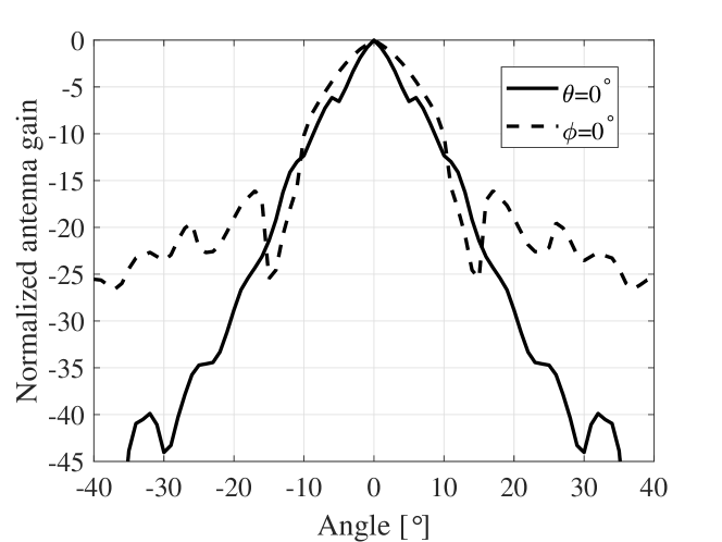
Figure 2: The used horn antenna pattern

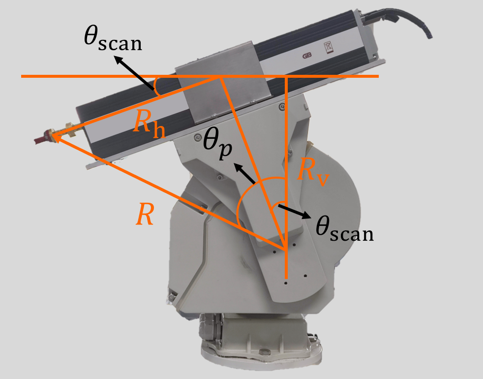
Figure 3: The rotator we use for direction-scan measurements.

III-A2 Scanning pattern of rotators

As derived in Appendix B, to calculate the ToAs using SWF assumption, the positions of Tx/Rx antennas in different scanning directions are needed. The rotator that we use is a typical mechanical rotator, as shown in Fig. 3.

When scanning different directions through mechanical rotations, the horn antenna forms a sphere with radius as $R$. Taking the center of the rotator as the origin, the position of the horn antenna can be expressed as

$$\bm{r}=R[\cos(\varphi_{p})\cos(\theta_{p}),\sin(\varphi_{p})\cos(\theta_{p}),\sin(\theta_{p})]^{\text{T}}$$ (31)

where $\varphi_{p}$ and $\theta_{p}$ are the relative azimuth angle and elevation angle of the horn antenna, respectively. Moreover, $R$ is the distance between the horn antenna and the rotation center. Based on the geometric relations shown in Fig. 3, these parameters can be expressed as

$$\varphi_{p} =\varphi_{\text{scan}}$$ (32)

$$\theta_{p} =\theta_{\text{scan}}+\arctan\left(\frac{R_{h}}{R_{v}}\right)$$ (33)

$$R =\sqrt{R_{h}^{2}+R_{v}^{2}}$$ (34)

where $\varphi_{\text{scan}}$ and $\theta_{\text{scan}}$ are the scanning azimuth and elevation angles, respectively. Additionally, $R_{h}$ and $R_{v}$ are the horizontal and vertical radius of the rotator, as shown in Fig. 3.

III-A3 Simulation parameters

For our simulations, the measurement band is selected as $300310\text{\,}\mathrm{G}\mathrm{H}\mathrm{z}$, with a $0.4\text{\,}\mathrm{M}\mathrm{H}\mathrm{z}$ sampling interval in the frequency domain. To save simulation time, we only consider the estimation of DoA while omitting DoDs of MPCs. Specifically, the Tx is assumed to be equipped with a omnidirectional antenna. In contrast, the Rx with a horn antenna is installed on a rotator, which scans the azimuth plane from $0^{\circ}$ to $360^{\circ}$ and the elevation plane from $-40^{\circ}$ to $40^{\circ}$ with a $10^{\circ}$ step. Furthermore, the horizontal and azimuth radius of the rotator are assumed to be $\sqrt{0.02}$, for which the antenna aperture is roughly as $2R=$$0.4\text{\,}\mathrm{m}$.

Based on the simulated MPC parameters, the CIR matrix can be constructed using (3), with the function $R(x,y)$ expressed in (A15). Moreover, the noise and phase terms in (3) are modeled as

$$W_{n_{t},n_{r}}[k] \sim\mathcal{CN}(0,\sigma_{N})$$ (35)

$$\phi_{n_{t},n_{r}} \sim\mathcal{N}(\phi,\sigma_{\phi})$$ (36)

where $\mathcal{CN}(\mu,\sigma)$ and $\mathcal{N}(\mu,\sigma)$ denote the complex Gaussian distribution and Gaussian distribution with mean value as $\mu$ and standard deviation as $\sigma$. Additionally, $\phi$ is the manually-selected initial phase of a MPC.

III-A4 Performance metric

To evaluate estimation accuracy of different algorithms, an average adjusted MCD is used, as

$$\overline{\text{MCD}}_{\text{ad}}=\frac{1}{L}\sum_{l=1}^{L}\min_{l^{\prime}}\text{MCD}_{\text{ad}}(\bm{\Theta}_{\text{T},l},\bm{\Theta}_{\text{E},l^{\prime}})$$ (37)

where $\bm{\Theta}_{\text{T},l}$ and $\bm{\Theta}_{\text{E},l^{\prime}}$ stand for the MPC parameters of the $l^{\text{th}}$ true MPC and the $(l^{\prime})^{\text{th}}$ estimated MPC, respectively. Moreover, $\text{MCD}_{\text{ad}}(\bm{\Theta}_{1},\bm{\Theta}_{2})$ is the adjusted MCD between two MPCs, calculated as

$$\begin{split}\text{MCD}_{\text{ad}}&(\bm{\Theta}_{1},\bm{\Theta}_{2})=\\ &\sqrt{\frac{(\tau_{1}-\tau_{2})^{2}}{\tau_{1}^{2}}+||\bm{\Omega}_{r,1}-\bm{\Omega}_{r,2}||^{2}+\frac{(\alpha_{1}-\alpha_{2})^{2}}{\alpha_{1}^{2}}}\end{split}$$ (38)

The adjusted MCD evaluates how similar two MPCs are, which quantifies the estimation error of channel parameter estimation algorithms. Therefore, the lower the adjusted MCD, the higher the accuracy of estimation algorithms. Specifically, we consider an adjusted MCD threshold as 0.01 to roughly judge whether the MPCs are estimated accurately or not.

III-B Single-path Simulations

To analyze the influences of measurement distance, noise power and phase errors, we consider that only one LoS path is received at the Rx. Two special cases are demonstrated, namely the on-grid case and off-grid case. The on-grid case means that the DoA of the LoS path falls exactly on the scanning direction grid, e.g., $\varphi_{r}=0^{\circ}$ and $\theta_{r}=0^{\circ}$. On the contrary, the off-grid case is to assume that the DoA of the LoS path is on the direction among adjacent grid points, e.g., $\varphi_{r}=5^{\circ}$ and $\theta_{r}=5^{\circ}$ in this work with a $10^{\circ}$ scanning step. Specifically, the parameters of the LoS path is expressed as

$$[\tau,\varphi_{r},\theta_{r},\alpha,\phi]=\begin{cases}[\frac{d}{c},0^{\circ},0^{\circ},\alpha_{\text{FS}}(f,d),0],&\text{on grid}\\ [\frac{d}{c},5^{\circ},5^{\circ},\alpha_{\text{FS}}(f,d),0],&\text{off grid}\end{cases}$$ (39)

where $d$ is the propagation distance of the LoS path and $c$ denotes the speed of light. Moreover, $\alpha_{\text{PL}}(f,d)$ is the path gain in free space at the distance $d$ with carrier frequency as $f$, which is given by the Friis’ law, as

$$\alpha_{\text{FS}}(f,d)=\frac{c}{4\pi fd}$$ (40)

Since only one MPC needs to be estimated, we consider one inner loop and one outer loop for both the SAGE and $\text{N}^{2}$-SAGE algorithms, while the noise elimination method takes the strongest temporal sample of the measured CIRs as the MPC. By varying the simulation setups, we can separately analyze the influences of near field, noise and random phase errors, which are discussed in detail as follows.

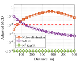
(a) Influences of near field

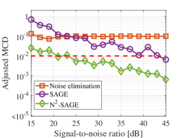
(b) Influence of noise.

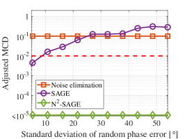
(c) Influence of phase errors.

Figure 4: Comparison among results of channel parameter estimation algorithms in the on-grid case.

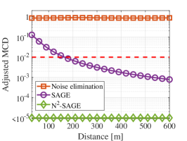
(a) Influences of near field

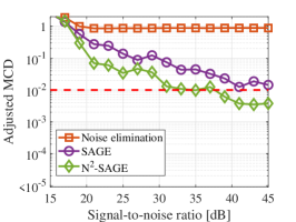
(b) Influence of noise.

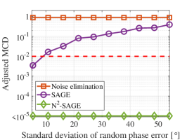
(c) Influence of phase errors.

Figure 5: Comparison among results of channel parameter estimation algorithms in the off-grid case.

Influences of near field

The measurement distance between Tx/Rx decides whether they are in near field or far field, which further affects the estimation performance of SAGE algorithms. To analyze this, the measurement distance varies from $30\text{\,}\mathrm{m}$ to $600\text{\,}\mathrm{m}$, while the background noise and phase errors are omitted, i.e., both $\sigma_{N}$ and $\sigma_{\phi}$ are set as zero. Note that for the scanning pattern and frequency band that we use, the Rayleigh distance is calculated as $320\text{\,}\mathrm{m}$.

The MCD between ground truth and estimated results in different measurement distances are shown in Fig. 4(a) and Fig. 5(a), based on which we can make several observations as follows. First, the noise elimination method performs badly compared to other two SAGE algorithms, especially in the off-grid case. In the on-grid case, as the distance increases, the estimation accuracy of noise elimination method first decreases and then increases. The reason is that as shown in the expressions of CIRs (A13), the ToA of the MPC is deviated as $\tau_{l}/(1+\Delta\tau\Delta f)$, which does not always fall on the temporal sample points of CIRs, resulting in inaccurate estimations of ToAs and path gains of MPCs. This deviation is dependent on the ToA and therefore dependent on the distances. Second, as the distance increases, smaller MCD can be observed for the estimation results based on SAGE algorithm, since Rx antenna gradually moves out of the near field. Specifically, for distance larger than $150\text{\,}\mathrm{m}$, the adjusted MCD based on SAGE algorithm is lower than 0.01, which is nearly half of the Rayleigh distance. Third, in contrast, the MCD values using $\text{N}^{2}$-SAGE algorithm remains very small for all distances, indicating the effectiveness of our proposed algorithm.

Influences of noise power

To observe the influences of background noise, the noise term is added with a standard deviation $\sigma_{N}$ of $\alpha^{2}/\text{SNR}$, where SNR denotes the signal-to-noise ratio (SNR) and changes from $15\text{\,}\mathrm{d}\mathrm{B}$ to $45\text{\,}\mathrm{d}\mathrm{B}$. To avoid the effects of near field and random phase errors, the distance is set as $600\text{\,}\mathrm{m}$ and the random phase is not added. To avoid the influence of randomness, for each SNR value, 50 simulations are conducted and the adjusted MCD values are averaged.

The influence of the background noise is shown in Fig. 4(b) and Fig. 5(b), from which we make statements as follows. First, the noise effects are stronger in the off-grid case, since in the off-grid case, the measured CIRs are much weaker due to antenna misalignment loss. Second, the performance of the noise elimination method rarely changes with the noise power. The reason is that for our considered SNR range, the signal is stronger than noises, for which the strongest temporal samples of CIRs, namely the estimation of noise elimination method, are not affected. Third, in both the on-grid and off-grid cases, the $\text{N}^{2}$-SAGE algorithm outperforms SAGE algorithm, with the estimation accuracy improved by around an order. This indicates that the usage of partial information in our proposed algorithm effectively alleviates the influences of noises.

Influences of random phase error

To analyze the effects of random phase errors, the standard deviation $\sigma_{\phi}$ ranges from $0^{\circ}$ to $54^{\circ}$. Moreover, the measurement distance is set as $600\text{\,}\mathrm{m}$ and background noise is not added. 50 simulations are conducted and the adjusted MCD values are averaged.

The estimation accuracy of different algorithms against phase errors are shown in Fig. 4(c) and Fig. 5(c). First, the noise elimination method is not affected by phase errors, since they do not involve any calculations but directly take the measured temporal samples as estimations. Second, the traditional SAGE algorithm is greatly affected by the phase errors in both on-grid and off-grid cases. As the standard deviation of phase errors increases, the performance of SAGE algorithm degrades. Specifically, when $\sigma_{\phi}$ is larger than $10^{\circ}$, the adjusted MCD obtained by SAGE is larger than 0.01, indicating significant inaccuracy. In the contrary, our proposed $\text{N}^{2}$-SAGE algorithm is well immune from the phase errors.

III-C Multi-path Simulations

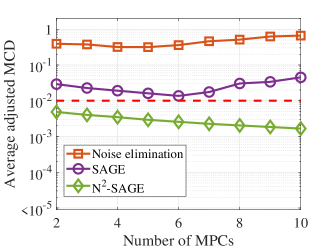
Figure 6: Comparison among results of channel parameter estimation algorithm based on multi-path simulations.

Apart from the three factors mentioned above, the inter-path interference, namely the $\sum_{l^{\prime}\neq l}^{L}\bm{E}_{l^{\prime}}^{m}$ in (4), could also degrade the performance of SAGE algorithms. To analyze this, we conduct ray-tracing simulations to obtain MPC parameters. Since we only use the ray-tracing simulations to obtain MPC parameters, rather than characterizing the THz channel, the calibration of the ray-tracing simulator, simulation layouts and setups are omitted here due to limitations of space.

After obtaining the MPC parameters based on the ray-tracing simulations, the $L$ strongest paths are used to reconstruct the CIRs in all scanning directions according to (3). The number of MPCs $L$ ranges from 2 to 10. To avoid influences of near field, noise and phase errors, which have already been examined in Sec. III-B, the CIRs are constructed based on PWF assumption and noise and phase errors are not added.

For fair comparison, both the SAGE algorithm and $\text{N}^{2}$-SAGE stop the inner loop when number of the estimated MPC exceeds $L+10$, and are considered to be converged after 5 outer loops. Moreover, similar to the single-path simulations, the noise elimination method takes the $L+10$ strongest temporal samples of CIRs as its estimations. The performance of channel parameter estimation algorithms based on multi-path simulations is shown in Fig. 6, from which we can make several observations as follows.

First, the accuracy of the noise elimination method is the worst, due to its limited resolutions. Second, the average adjusted MCD values based on SAGE algorithm is around 1 order larger than those of $\text{N}^{2}$-SAGE algorithm, indicating that the $\text{N}^{2}$-SAGE algorithm is well immune from the inter-path interference while the SAGE algorithm suffers. The main reason is that the inter-path interference could result in wrong estimations of MPC phases, which further introduce accumulated phase errors. As the $\text{N}^{2}$-SAGE is immune to phase errors, its performance barely degenerates, while the SAGE algorithm is greatly degraded.

IV Estimation and Channel Characterization Results Using Real Measured Data

In this section, the estimation performance of the proposed $\text{N}^{2}$-SAGE algorithm is evaluated using real measured data in an indoor corridor scenario, as reported in [16]. The estimation accuracy of the PDAP is compared with existing channel parameter estimation algorithms. Furthermore, based on the estimated MPC parameters, channel characteristics are calculated, including path loss, K-factor, delay and angular spreads.

IV-A Measurement Campaign and Parameter Setups

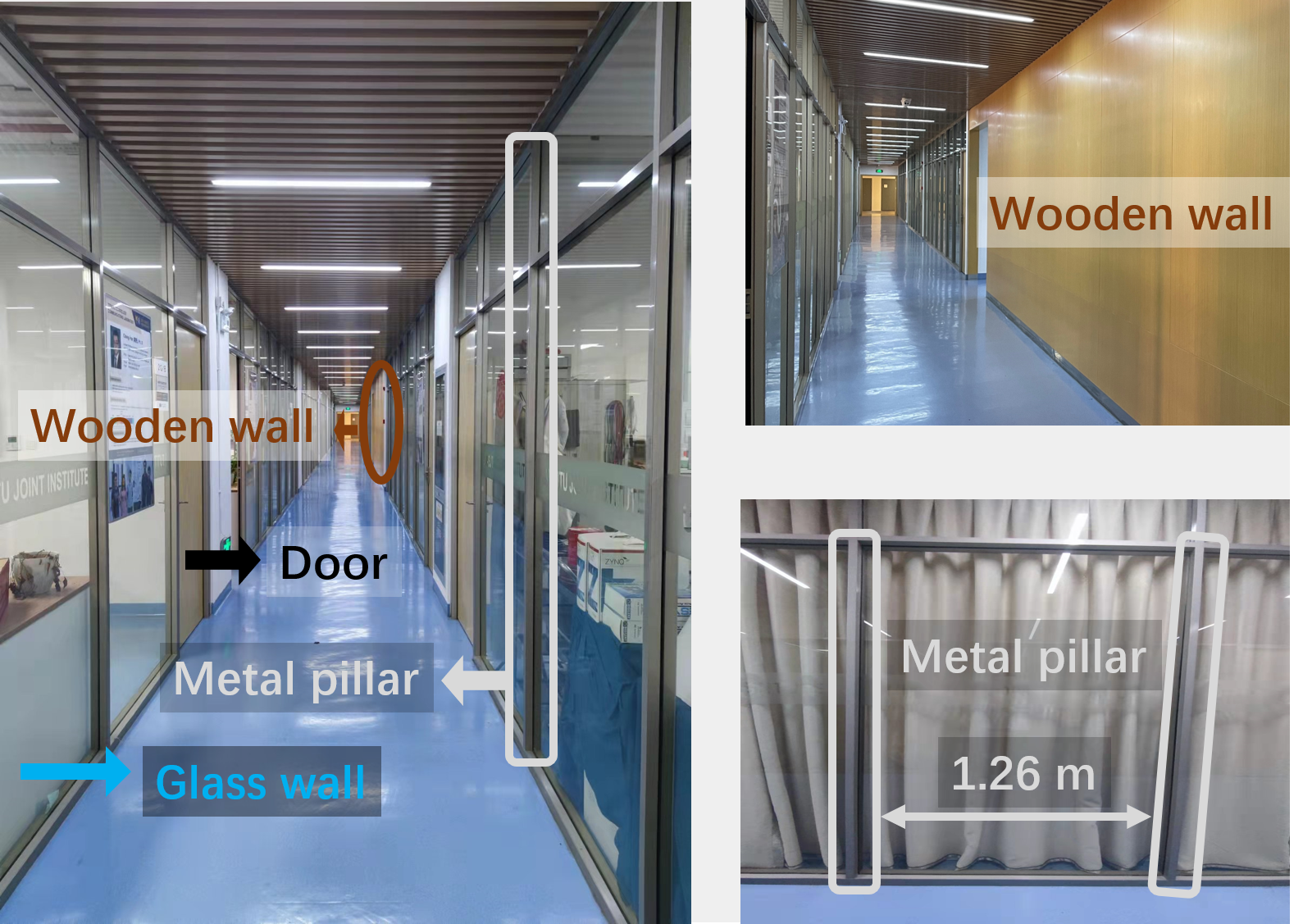
(a) Pictures of the corridor.

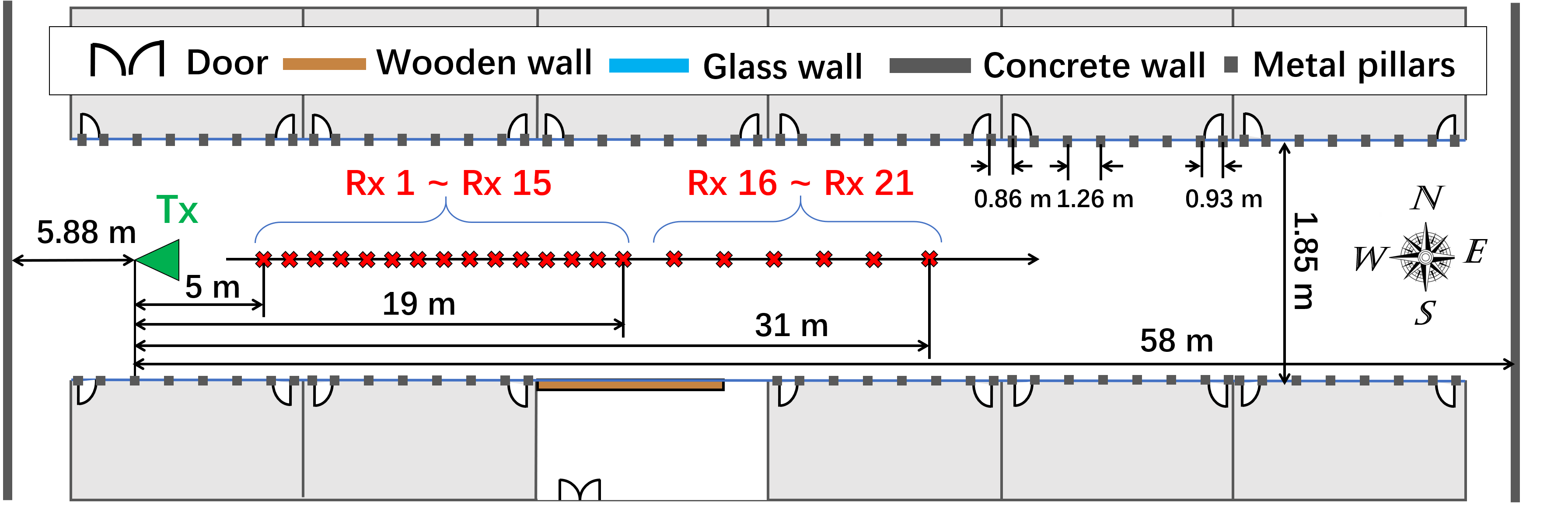
(b) Bird’s eye view.

Figure 7: The layout of the measurement campaign conducted in the corridor [16]

The channel measurement campaign is conducted in $306321\text{\,}\mathrm{G}\mathrm{H}\mathrm{z}$ in a typical indoor corridor scenario, as shown in Fig. 7. Both sides of the corridor are furnished with glass walls, which are connected together with metal pillars. The Tx/Rx separation distance ranges from $5\text{\,}\mathrm{m}$ to $31\text{\,}\mathrm{m}$ with 21 receiver positions. Moreover, the transmitter antenna remains static, while the Rx antenna scans the spatial domain, as $-20\sim 20^{\circ}$ in elevation plane and $0\sim 360^{\circ}$ in azimuth plane, both with a rotation step of $10^{\circ}$. Therefore, we estimate the DoAs of MPCs, while the DoDs of MPCs are omitted. The antenna pattern and scanning pattern of rotators are mentioned in Sec. III-A. For detailed description of the channel sounders, measurement setups, and measurement deployments, please refer to [16].

Based on the measured data, we estimate MPCs with path gains that are larger than a certain threshold $\alpha_{\text{th}}$, which is determined as

$$\alpha_{\text{th}}=\max(\alpha_{1}/10000,10^{-7.25})$$ (41)

where $\alpha_{1}$ denoting the largest path gain of estimated MPCs and the number $10000$ indicating a $40\text{\,}\mathrm{d}\mathrm{B}$ dynamic range. Moreover, the number $10^{-7.25}$, corresponding to a path loss threshold as $-145\text{\,}\mathrm{d}\mathrm{B}$, is selected according to our experience to avoid effects from noises.

For noise elimination method, all temporal samples of CIRs that are stronger than $\alpha_{\text{th}}$ are regarded as MPCs. For both SAGE and $\text{N}^{2}$-SAGE algorithms, their inner loop stops when the estimated path gain is lower than $\alpha_{\text{th}}$. Moreover, due to the combination of near field effects, noises, and random phase errors, the SAGE algorithm will gradually diverge with many outer loops. Therefore, only one outer loop is considered for SAGE algorithm. In contrast, the $\text{N}^{2}$-SAGE algorithm is regarded as converged when (30) is satisfied with $\text{MCD}_{\text{th}}$ and $r_{\text{th}}$ selected as 0.1 and 0.9, respectively, or number of outer loops exceeds 10.

IV-B Estimation Accuracy of PDAP

To evaluate the accuracy of the estimated MPC parameters, we compare measured PDAPs with reconstructed PDAPs based on estimated MPC parameters using different channel parameter estimation algorithms, which are obtained as

$$\text{P}_{n_{r}}^{\text{M}}[\text{dB}] =20\log_{10}\left|h_{n_{r}}^{\text{M}}\right|,$$ (42)

$$\text{P}_{n_{r}}^{\text{E}}[\text{dB}] =20\log_{10}\left|h_{n_{r}}^{\text{E}}\right|$$ (43)

where $h_{n_{r}}^{\text{M}}$ is the measured CIR at the $(n_{r})^{\text{th}}$ scanning direction of Rx. Moreover, $h_{n_{r}}^{\text{E}}$ is the reconstructed CIR in the $(n_{r})^{\text{th}}$ scanning direction based on the estimated MPC parameters.

Furthermore, the estimation accuracy is evaluated in terms of root mean square error (RMSE) between the measured and reconstructed PDAPs, as

$$\text{RMSE}~{}[\text{dB}]=\sqrt{\frac{\sum_{n_{r}}\sum_{i\in\bm{I}_{n_{r}}}\left(\text{P}_{\text{M},n_{r}}[i]-\text{P}_{\text{E},n_{r}}[i]\right)^{2}}{\sum_{n_{r}}\sum_{i\in\bm{I}_{n_{r}}}1}}$$ (44)

where $\bm{I}_{n_{r}}$ denotes the time indexes of PDAP samples that are larger than the power threshold $P_{\text{th}}$, where $P_{\text{th}}=20\log_{10}\left|\alpha_{\text{th}}\right|$. Moreover, $\sum_{n_{r}}\sum_{i\in\bm{I}_{n_{r}}}1$ represents the overall number of interested sample points of PDAPs.

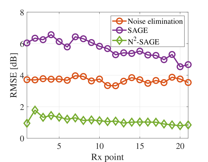
Figure 8: RMSE between measured PDAPs and reconstructed PDAPs using SAGE algorithms.

The RMSEs between the measured PDAPs and reconstructed PDAPs are shown in Fig. 8, from which we can make several observations as follows. First, the RMSE values based on SAGE algorithm is the worst among results of the three methods. The reason is that due to the influences of near fields, noises, and random phase errors, the SAGE algorithm shows bad estimation performance and produces wrong estimations, resulting in inaccurate PDAPs. Second, the estimation results of the noise elimination method are also inaccurate, with RMSE values around $4\text{\,}\mathrm{d}\mathrm{B}$, since it fails to decouple the antenna effects. Third, in contrast, our proposed $\text{N}^{2}$-SAGE shows high accuracy when applied to real measured data, with RMSE values around $1\text{\,}\mathrm{d}\mathrm{B}$. The comparison reveals the effectiveness of our proposed $\text{N}^{2}$-SAGE algorithm in mmWave and THz direction-scan measurements.

IV-C Channel Characteristics

The estimated MPC parameters directly affect the calculations of channel characteristics. In this part, we calculate and analyze the channel characteristics based on different channel parameter estimation algorithms, including path loss, K-factor, delay and angular spreads.

IV-C1 Path loss

TABLE I: Channel characteristics calculated based on different channel parameter estimation algorithms in the corridor scenario.

TABLE II: Channel characteristics distribution parameters calculated based on different channel parameter estimation algorithms in the corridor scenario.

The path loss, also known as large-scale fading, is of great importance to evaluate the link budget when designing communication systems. Specifically, in our channel measurement campaigns, the path loss is calculated as the summation of the received power of all MPCs, as

$$\text{PL}~{}[\text{dB}]=-10\log_{10}(\sum_{l=1}^{L}{\left|\alpha_{l}\right|^{2}})$$ (45)

where $\alpha_{l}$ denotes path gain of the $l^{\text{th}}$ path.

Generally, the path loss is modeled as a linear function with respect to the logarithm of the Euclidean distance between Tx and Rx. In line with this, a close-in (CI) free space reference distance model is used, which is defined as

$$\text{PL}^{\text{CI}}[\text{dB}]=10n\log_{10}\frac{d}{d_{0}}+\text{FSPL}(d_{0})$$ (46)

where $n$ stands for the path loss exponent (PLE) of the CI model. Additionally, $d$ is the Euclidean distance between Tx and Rx and $d_{0}$ stands for the reference distance, which is selected as $1\text{\,}\mathrm{m}$ here. $\text{FSPL}(d_{0})$ denotes the free space path loss at distance $d_{0}$ and is calculated as $20\log_{10}(\alpha_{\text{FS}}(f,d_{0}))$ with $\alpha_{\text{FS}}(f,d)$ expressed in (40).

The path loss results are shown in Table I, where the PLEs are extracted in Table II. First, the path loss results of noise elimination method and $\text{N}^{2}$-SAGE algorithm are close. The reason is that for a certain MPC, its duplicates in all scanning directions are treated as MPCs by the noise elimination method, the summation of whose power is close to its real power. As a result, similar path loss results are observed for noise elimination and $\text{N}^{2}$-SAGE algorithm. Second, the SAGE algorithm greatly overestimates the path loss by around $4\text{\,}\mathrm{d}\mathrm{B}$, which indicates its inefficiency in mmWave and THz direction-scan measurement campaigns. Third, with the $\text{N}^{2}$-SAGE algorithm, the path loss in the indoor corridor scenario at $300\text{\,}\mathrm{G}\mathrm{H}\mathrm{z}$ is characterized, with a PLE around 1.45. The small PLE comes from the significant diffusely scattering from metal pillars in both sizes of the corridor, as discussed with propagation analysis in [16].

IV-C2 K-factor

Defined as the ratio between the power of the strongest MPC and the power of other MPCs, the K-factor evaluates how dominant the strongest MPC is. However, due to factors such as inaccurate calibrations, inaccurate estimations, etc., it is very hard to completely extract the strongest MPC from the measured results. Therefore, instead of using the traditional definition, we calculate the K-factors by the power ratio between the power of MPCs that are very close to the strongest MPC and power of other MPCs, as

$$\text{KF}[\text{dB}]=10\log_{10}\frac{\sum_{l\in\bm{L}_{LoS}}\left|\alpha_{l}\right|^{2}}{\sum_{l\notin\bm{L}_{LoS}}\left|\alpha_{l}\right|^{2}}$$ (47)

where $\bm{L}_{LoS}$ is determined as

$$\bm{L}_{LoS}=\{l;\text{MCD}(\bm{\Theta}_{l},\bm{\Theta}_{1})<\text{MCD}_{\text{th},\text{KF}}\}$$ (48)

where the threshold $\text{MCD}_{\text{th},\text{KF}}$ is selected as 0.15.

Comparing the results using different estimation methods, the K-factor values based on noise elimination method and SAGE algorithm are much smaller than those estimated using $\text{N}^{2}$-SAGE algorithm. The reason behind this is two-fold. On one hand, the estimated MPCs of noise elimination method include duplicates of MPCs due to effects of antennas, resulting in smaller K-factor values. On the other hand, for a certain MPC, the SAGE algorithm fails to accurately estimate the parameters of it and thus can not eliminate its effects with the PIC in (4), which further results many fake MPCs with significant power. Therefore, the K-factor values based on SAGE algorithm are also greatly underestimated. Furthermore, with the $\text{N}^{2}$-SAGE algorithm, the K-factor values in our measured results are calculated averagely as $0.73\text{\,}\mathrm{d}\mathrm{B}$, which attributes to the significant scattering from metal pillars.

IV-C3 Delay and angular spreads

The power of the MPCs disperses in both the temporal and spatial domains, which is evaluated by the delay and angular spreads. The delay spread, azimuth spread of arrival (ASA) and the elevation spread of arrival (ESA) are summarized in Table I, from which we make several observations. First, for the delay spread values, compared to the results using $\text{N}^{2}$-SAGE algorithm, the results using noise elimination method and SAGE algorithm are smaller. Second, the ASA results based on noise elimination method and SAGE algorithm are smaller than those based on $\text{N}^{2}$-SAGE algorithm, while the ESA values are larger. The reason behind these inaccurate spread values is that by using the noise elimination method and SAGE algorithm, for a certain path, significant fake MPCs with ToA and DoA around the real path are obtained. As a result, the delay spread is underestimated, while the angular spreads are misled to be closer to $10\sim 20^{\circ}$. Those angular spread values, which are actually larger than this range, tend to be smaller, while others that are expected to be smaller grow. Third, by using the $\text{N}^{2}$-SAGE algorithm, the delay spread is averagely calculated as $21.38\text{\,}\mathrm{n}\mathrm{s}$, while the average ASA and ESA values are $39.81^{\circ}$ and $5.89^{\circ}$, respectively. The large spread values reveals the strong multi-path effects from diffusely scattering from metal pillars on both sides of the corridor.

V Conclusion

In this paper, we proposed a novel narrow-beam near-field space-alternating generalized expectation-maximization ($\text{N}^{2}$-SAGE) algorithm by carefully considering the properties of mmWave and THz direction-scan measurements, such as near field propagation, narrow antenna beams and asynchronous measurements in different scanning directions. The spherical wave front in near fields couples the estimation of delay and angles together, which is decomposed with a two-phase estimation process to reduce the time and computation resource consumption. Considering the narrow antenna beams, the usage of partial information alleviate influence of background noises. By treating phases of MPCs as scanning-direction-dependent variables, the proposed algorithm is well immune to possible phase errors attributing to asynchronous measurements. Furthermore, we evaluated the performance of the proposed algorithm and compared with traditional SAGE algorithm and widely-used noise elimination method, based on simulations. Influences of several factors, such as near field, noise power, random phase errors, as well as number of MPCs, are fully investigated. Last but not least, we applied the proposed $\text{N}^{2}$-SAGE algorithm in real measured data, which were further compared with results based on other methods.

Particularly, key observations are highlighted as follows. First, with carefully considering the typical features of mmWave and THz direction-scan measurements, namely the near field effects, narrow antenna beams and possible phase shifts, the proposed $\text{N}^{2}$-SAGE algorithm greatly outperforms existing algorithms in terms of estimation accuracy. Second, without using the $\text{N}^{2}$-SAGE algorithm, inaccurate channel characterization results are produced based on noise elimination method and SAGE algorithm, such as larger path loss, smaller K-factor, smaller delay spread, smaller azimuth angle spread, and large elevation angle spread. Third, based on the $\text{N}^{2}$-SAGE algorithm, the channels in the indoor corridor scenario at $300\text{\,}\mathrm{G}\mathrm{H}\mathrm{z}$ are characterized, where we observe a PLE of 1.45, mean K-factor of $0.73\text{\,}\mathrm{d}\mathrm{B}$, average delay spread of $21.38\text{\,}\mathrm{n}\mathrm{s}$, average ASA and ESA of $39.81^{\circ}$ and $5.89^{\circ}$, respectively. In general, the proposed $\text{N}^{2}$-SAGE algorithm can be used to accurately estimate the MPC parameters in mmWave and THz direction-scan measurements, which is helpful for channel modeling and system design for mmWave and THz communications.

Appendix A General Form of Channel Impulse Response

There are mainly three kinds of methods to measure the mmWave and THz channels, namely pulse-based time domain method, correlation-based time domain method, and vector network analyzer (VNA)-based frequency domain method [21]. In the following part, we show that for all three methods, the measured CIR can be expressed in the same form.

A-A Pulse-based Method

For pulse-based time domain method, the basic idea is to transmit a sharp pulse, whose shape is close to a Dirac function, and the received signal is directly treated as the CIR. Specifically, the sharp pulse is transmitted at time $t_{0}$, denoted as $u(t-t_{0})$, and the received signal is expressed as

$$\begin{split}y(t)=\sum_{l=1}^{L}s^{\prime}_{l}u(t-t_{0}-\tau_{l})+w(t)\end{split}$$ (A1)

where $s^{\prime}_{l}=\alpha_{l}c_{t}(\bm{\Omega}_{t,l})c_{r}(\bm{\Omega}_{r,l})\text{e}^{j\phi_{l}}$ denote part of the signal that is not dependent on time. Moreover, $\alpha_{l},\tau_{l},\bm{\Omega}_{t,l},\bm{\Omega}_{r,l},\phi_{l}$ denote the real-valued path gain, ToA, DoD, DoA, and phase of the $l^{\text{th}}$ MPC, respectively. Additionally, $L$ is the number of MPCs. Moreover, $w(\cdot)$ represents the white Gaussian noise components. Furthermore, $c_{t}(\bm{\Omega}_{t,l})$ and $c_{r}(\bm{\Omega}_{r,l})$ stand for the radiation pattern of Tx and Rx horn antennas, respectively. Furthermore, by transforming the received signal into delay domain with $\tau=t-t_{0}$, the CIR is

$$\begin{split}h(\tau)=\sum_{l=1}^{L}s^{\prime}_{l}u(\tau-\tau_{l})+w(\tau)\end{split}$$ (A2)

With temporal sampling, the discrete CIR is expressed as

$$\begin{split}h[i]=\sum_{l=1}^{L}s^{\prime}_{l}u((i-1)\Delta\tau-\tau_{l})+w[i]\end{split}$$ (A3)

where $i$ and $\Delta\tau$ denote the sampling index and sampling interval in the time domain.

A-B Correlation-based Method

In correlation-based method, the auto-correlation function of the transmitted signal is close to a Dirac function. Therefore, after the received signal passing a correlator, the CIR is obtained, as

$$\begin{split}h(\tau)&=\int_{0}^{T_{c}}y(t)u^{*}(t-t_{0}-\tau)dt\\ &=\sum_{l=1}^{L}s^{\prime}_{l}R_{u}(\tau-\tau_{l})+w(t)\end{split}$$ (A4)

where $T_{c}$ denotes the signal duration of $u(t)$. Moreover, $R_{u}(\tau)=u(t)u^{*}(t-\tau)$ is the auto-correlation function of the transmitted signal. Moreover, $(\cdot)^{*}$ stands for the conjugate operation of complex numbers.

Again, with temporal sampling, the discrete CIR is expressed as

$$h[i]=\sum_{l=1}^{L}s^{\prime}_{l}R_{u}((i-1)\Delta\tau-\tau_{l})+w[i]$$ (A5)

A-C VNA-based Method

Different from the above-mentioned two time-domain methods, the VNA-based method measures the channel transfer functions (CTFs) of wireless channels and the CIRs are obtained through inverse discrete Fourier transform (IDFT). Specifically, the CTF of wireless channels can be expressed as

$$H(f)=\sum_{l=1}^{L}s^{\prime}_{l}\text{e}^{-j2\pi f\tau_{l}}+W(f)$$ (A6)

By scanning the interested frequency band with VNA, the discrete CTF is measured, as

$$H[k]=\sum_{l=1}^{L}s^{\prime}_{l}\text{e}^{-j2\pi f_{k}\tau_{l}}+W[k]$$ (A7)

where $f_{k}$ denotes the carrier frequency at the $k^{\text{th}}$ sampling point, i.e., $f_{k}=f_{1}+(k-1)\Delta f$. $f_{1}$ and $f_{2}$ represent the lower and upper frequencies of the measured band. $\Delta f$ is the sampling interval in the frequency domain.

Taking IDFT on the measured CTF, we obtain

$$\begin{split}h[i]=\sum_{l=1}^{L}s^{\prime}_{l}\text{IDFT}[\text{e}^{-j2\pi f_{k}\tau_{l}}]+w[i]\end{split}$$ (A8)

Furthermore, by using the definitions of IDFT and denoting the term $\text{IDFT}[\text{e}^{-j2\pi f_{k}\tau_{l}}]$ as $v_{l}$, we have

$$v_{l}[i] =\frac{1}{K}\sum_{k=1}^{K}\text{e}^{-j2\pi f_{k}\tau_{l}}\text{e}^{j2\pi(k-1)(i-1)/K}$$ (A9a)

$$=\frac{\text{e}^{j\varphi_{l}}}{K}\sum_{k=1}^{K}\text{e}^{-j2\pi((k-1)\Delta f\tau_{l}-(k-1)(i-1)/K)}$$ (A9b)

$$=\frac{\text{e}^{j{\varphi}_{l}}}{K}\sum_{k=1}^{K}\text{e}^{-j2\pi((k-1)\Delta f{\tau_{l}}-(k-1)(i-1)\frac{\Delta\tau\Delta f}{1+\Delta\tau\Delta f})}$$ (A9c)

$$=\frac{\text{e}^{j{\varphi}_{l}}}{K}\sum_{k=1}^{K}\text{e}^{-j2\pi(k-1)\Delta f\Delta_{\tau}((i-1)\Delta\tau,\tau_{l})}$$ (A9d)

where (A9c) comes from the fact that $1/(K-1)=\Delta f\Delta\tau$. Besides, $\Delta_{\tau}(x,y)=y-x/a$ with $a=1+\Delta\tau\Delta f$. Moreover, the additional phase term ${\varphi}_{l}$ is $-2\pi f_{1}{\tau}_{l}$.

When $\Delta f\Delta_{\tau}((i-1)\Delta\tau,\tau_{l})=0$, it is obvious that $v_{l}[i]=\text{e}^{j{\varphi}_{l}}$. When $\Delta f\Delta_{\tau}((i-1)\Delta\tau,\tau_{l})\neq 0$, By utilizing the properties of geometric series, we obtain

$$v_{l}[i]=\frac{\text{e}^{j{\varphi}_{l}}}{K} \frac{1-\text{e}^{-j2\pi K\Delta f\Delta_{\tau}((i-1)\Delta\tau,\tau_{l})}}{1-\text{e}^{-j2\pi\Delta f\Delta_{\tau}((i-1)\Delta\tau,\tau_{l})}}$$ (A10a)

$$=\frac{\text{e}^{j{\varphi}_{l}}}{K} \frac{\text{e}^{-j\pi K\Delta f\Delta_{\tau}((i-1)\Delta\tau,\tau_{l})}}{\text{e}^{-j\pi\Delta f\Delta_{\tau}((i-1)\Delta\tau,\tau_{l})}}\cdot$$ (A10b)

$$\frac{\sin{(\pi K\Delta f\Delta_{\tau}((i-1)\Delta\tau,\tau_{l}))}}{\sin{(\pi\Delta f\Delta_{\tau}((i-1)\Delta\tau,\tau_{l}))}}$$ (A10c)

Therefore, $v_{l}[i]$ can be expressed as

$$v_{l}[i]=\text{e}^{j\varphi^{\prime}_{l}}g_{K}(\pi\Delta f\Delta_{\tau}((i-1)\Delta\tau,\tau_{l}))$$ (A11)

where the phase term is ${\varphi}^{\prime}_{l}={\varphi}_{l}-\pi(K-1)\Delta f\Delta_{\tau}((i-1)\Delta\tau,\tau_{l})$. Moreover, $g_{K}(x)$ is of the form as

$$g_{K}(x)=\begin{cases}1,&x=0\\ \frac{\sin(Kx)}{K\sin(x)},&x\neq 0\end{cases}$$ (A12)

Utilizing (A11) in (A8), we have

$$\begin{split}h[i]=\sum_{l=1}^{L}s^{\prime}_{l}g_{K}(\pi\Delta f\Delta_{\tau}((i-1)\Delta\tau,\tau_{l}))\text{e}^{j\varphi^{\prime}_{l}}+w^{\prime}[i]\end{split}$$ (A13)

A-D Summary

The measured CIRs with different methods in (A3), (A5), and (A13) can be expressed with a general form, as

$$h[i]=\sum_{l=1}^{L}s^{\prime}_{l}R((i-1)\Delta\tau,\tau_{l})+w[i]$$ (A14)

where the function $R(x,y)$ is of the form as

$$\begin{split}R&(x,y)=\\ &\begin{cases}u(x-y),&\text{pulse-based}\\ R_{u}(x-y),&\text{correlation-based}\\ g_{K}(\pi\Delta f\Delta_{\tau}(x,y))\text{e}^{j\varphi^{\prime}_{l}},&\text{VNA-based}\end{cases}\end{split}$$ (A15)

The function $R(x,y)$ has the property that the maximum of its absolute value occurs when $x-y$ is zero (for time-domain methods) or very close to zero (for VNA-based method).

Appendix B Delay Difference Calculation Using Spherical Wave Front

In direction-scan measurements, the positions of Tx/Rx antennas change for different pointing directions, due to rotations of Tx/Rx modules. Therefore, for a certain MPC, it travels past different propagation distance when Tx/Rx antennas point to different directions, resulting in different observed ToAs.

We first consider a single-input multi-output (SIMO) system. By treating the rotation center of the Rx rotators as the origin, the position of the Rx antenna for the $(n_{r})^{\text{th}}$ scanning direction is represented as $\bm{r}_{\text{Rx},n_{r}}$. Furthermore, we assume that a MPC is received with time-of-arrival (ToA) and direction-of-arrival (DoA) as $\tau$ and $\bm{\Omega}_{r}$. To calculate the observed ToA of this MPC in the $(n_{r})^{\text{th}}$ scanning direction, we introduce the concept of the virtual transmitter (vTx) position, which is expressed as

$$\bm{r}_{\text{Tx}}^{\text{v}}=c\tau\bm{\Omega}_{r}$$ (A1)

where $c$ is the speed of light. Moreover, the DoA vector is determined be the azimuth angle-of-arrival (AoA) $\varphi_{r}$ and elevation angle-of-arrival (EoA) $\theta_{r}$, as

$$\bm{\Omega}_{r}=[\cos(\varphi_{r})\cos(\theta_{r}),\sin(\varphi_{r})\cos(\theta_{r}),\sin(\theta_{r})]^{\text{T}}$$ (A2)

In other words, we assume that there is a virtual transmitter at the position $\bm{r}_{\text{Tx}}^{\text{v}}$ and the interested MPC is just a line-of-sight (LoS) MPC received at the Rx. Note that this assumption is only valid for specular reflected paths and not accurate for diffuse scattering and diffracted paths. However, in mmWave and THz channels, specular reflected paths are much stronger than other multipath components, for which we only consider the specular reflected paths while omit influences from other MPCs.

Based on the virtual transmitter position, the observed ToA in the $(n_{r})^{\text{th}}$ scanning direction is simply calculated as

$$f_{\tau,r}(\tau,\bm{\Omega}_{r},n_{r})=\frac{||\bm{r}_{\text{Tx}}^{\text{v}}-\bm{r}_{\text{Rx},n_{r}}||}{c}$$ (A3)

where $||\cdot||$ is the norm of a vector.

Similarly, for a multi-input single-output (MISO) system, the observed ToA can be calculated by invoking the virtual receivers, as

$$f_{\tau,t}(\tau,\bm{\Omega}_{t},n_{t})=\frac{||\bm{r}_{\text{Rx}}^{\text{v}}-\bm{r}_{\text{Tx},n_{t}}||}{c}$$ (A4)

where the virtual receiver position simply equals to $c\tau\bm{\Omega}_{t}$. Moreover, $\bm{r}_{\text{Tx},n_{t}}$ is the position of the Tx antenna for the $(n_{t})^{\text{th}}$ scanning direction, by denoting the rotation center of Tx rotator as the origin.

Treating multi-input multi-output systems as compositions of SIMO and MISO systems, the observed ToA is expressed as

$$f_{\tau}(\tau,\bm{\Omega}_{t},\bm{\Omega}_{r},n_{t},n_{r})=f_{\tau,r}(f_{\tau,t}\left(\tau,\bm{\Omega}_{t},n_{t}),\bm{\Omega}_{r},n_{r}\right)$$ (A5)

Reversely, by combining (A3)-(A5), if the observed ToA in the $(n_{t})^{\text{th}}$ Tx scanning direction and $(n_{r})^{\text{th}}$ scanning direction is $\tau_{0}$, the true ToA can be expressed as

$$\begin{split}f^{-1}_{\tau}&(\tau_{0},n_{t},n_{r},\bm{\Omega}_{t},\bm{\Omega}_{r})=\frac{||\bm{r}_{\text{Rx},n_{r}}+c(\bm{r}_{\text{Tx},n_{t}}+c\tau_{0}\bm{\Omega}_{t})\bm{\Omega}_{r}||}{c}\end{split}$$ (A6)

References

- [1] Z. Chen, C. Han, Y. Wu, L. Li, C. Huang, Z. Zhang, G. Wang, and W. Tong, “Terahertz wireless communications for 2030 and beyond: A cutting-edge frontier,” IEEE Commun. Mag., vol. 59, no. 11, pp. 66–72, 2021.
- [2] M. Xiao, S. Mumtaz, Y. Huang, L. Dai, Y. Li, M. Matthaiou, G. K. Karagiannidis, E. Björnson, K. Yang, C.-L. I, and A. Ghosh, “Millimeter wave communications for future mobile networks,” IEEE J. Sel. Areas Commun., vol. 35, no. 9, pp. 1909–1935, 2017.
- [3] I. F. Akyildiz, C. Han, and S. Nie, “Combating the distance problem in the millimeter wave and terahertz frequency bands,” IEEE Commun. Mag., vol. 56, no. 6, pp. 102–108, 2018.
- [4] T. S. Rappaport, Y. Xing, O. Kanhere, S. Ju, A. Madanayake, S. Mandal, A. Alkhateeb, and G. C. Trichopoulos, “Wireless communications and applications above 100 GHz: Opportunities and challenges for 6G and beyond,” IEEE Access, vol. 7, pp. 78 729–78 757, 2019.
- [5] M. Jacob, S. Priebe, R. Dickhoff, T. Kleine-Ostmann, T. Schrader, and T. Kürner, “Diffraction in mm and Sub-mm Wave Indoor Propagation Channels,” IEEE Trans. Microw. Theory Techn., vol. 60, no. 3, pp. 833–844, Jan. 2012.
- [6] C. Jansen, S. Priebe, C. Moller, M. Jacob, H. Dierke, M. Koch, and T. Kurner, “Diffuse Scattering From Rough Surfaces in THz Communication Channels,” IEEE Trans. THz Sci. Technol., vol. 1, no. 2, pp. 462–472, 2011.
- [7] S. Ju, S. H. A. Shah, M. A. Javed, J. Li, G. Palteru, J. Robin, Y. Xing, O. Kanhere, and T. S. Rappaport, “Scattering mechanisms and modeling for terahertz wireless communications,” in Proc. of IEEE ICC, pp. 1–7, 2019.
- [8] F. Erden, O. Ozdemir, and I. Guvenc, “28 GHz mmWave Channel Measurements and Modeling in a Library Environment,” in Proc. of IEEE RWS, pp. 52–55, 2020.
- [9] T. S. Rappaport, G. R. MacCartney, M. K. Samimi, and S. Sun, “Wideband millimeter-wave propagation measurements and channel models for future wireless communication system design,” IEEE Trans. Commun., vol. 63, no. 9, pp. 3029–3056, 2015.
- [10] Y. Xing, T. S. Rappaport, and A. Ghosh, “Millimeter Wave and Sub-THz Indoor Radio Propagation Channel Measurements, Models, and Comparisons in an Office Environment,” IEEE Commun. Lett., vol. 25, no. 10, pp. 3151–3155, 2021.
- [11] S. Ju, Y. Xing, O. Kanhere, and T. S. Rappaport, “Millimeter wave and sub-terahertz spatial statistical channel model for an indoor office building,” IEEE J. Sel. Areas Commun., vol. 39, no. 6, pp. 1561–1575, 2021.
- [12] Y. Chen, Y. Li, C. Han, Z. Yu, and G. Wang, “Channel Measurement and Ray-Tracing-Statistical Hybrid Modeling for Low-Terahertz Indoor Communications,” IEEE Trans. Wireless Commun., vol. 20, no. 12, pp. 8163–8176, 2021.
- [13] C.-L. Cheng and A. Zajić, “Characterization of propagation phenomena relevant for 300 GHz wireless data center links,” IEEE Trans. Antennas Propag., vol. 68, no. 2, pp. 1074–1087, 2019.
- [14] S. Priebe, C. Jastrow, M. Jacob, T. Kleine-Ostmann, T. Schrader, and T. Kürner, “Channel and propagation measurements at 300 GHz,” IEEE Trans. Antennas Propag., vol. 59, no. 5, pp. 1688–1698, 2011.
- [15] J. He, Y. Chen, Y. Wang, Z. Yu, and C. Han, “Channel Measurement and Path-Loss Characterization for Low-Terahertz Indoor Scenarios,” in Proc. of IEEE ICC Workshops, pp. 1–6, 2021.
- [16] Y. Li, Y. Wang, Y. Chen, Z. Yu, and C. Han, “Channel Measurement and Analysis in an Indoor Corridor Scenario at 300 GHz,” in Proc. of IEEE ICC, 2022.
- [17] N. A. Abbasi, J. Gomez-Ponce, R. Kondaveti, S. M. Shaikbepari, S. Rao, S. Abu-Surra, G. Xu, C. Zhang, and A. F. Molisch, “Thz band channel measurements and statistical modeling for urban d2d environments,” IEEE Transactions on Wireless Communications, pp. 1–1, 2022.
- [18] Y. Xing and T. S. Rappaport, “Propagation measurements and path loss models for sub-thz in urban microcells,” in Proc. of IEEE ICC, pp. 1–6, 2021.
- [19] J. M. Eckhardt, V. Petrov, D. Moltchanov, Y. Koucheryavy, and T. Kürner, “Channel Measurements and Modeling for Low-Terahertz Band Vehicular Communications,” IEEE J. Sel. Areas Commun., vol. 39, no. 6, pp. 1590–1603, 2021.
- [20] N. Abbasi, J. Gómez, S. Shaikbepari, S. Rao, R. Kondaveti, S. Abu-Surra, G. Xu, C. Zhang, and A. Molisch, “Ultra-Wideband Double Directional Channel Measurements for THz Communications in Urban Environments,” in Proc. of IEEE ICC, pp. 1–6, Jun. 2021.
- [21] C. Han, Y. Wang, Y. Li, Y. Chen, N. A. Abbasi, T. Kürner, and A. F. Molisch, “Terahertz wireless channels: A holistic survey on measurement, modeling, and analysis,” IEEE Commun. Surveys Tuts., vol. 24, no. 3, pp. 1670–1707, 2022.
- [22] B. H. Fleury, M. Tschudin, R. Heddergott, D. Dahlhaus, and K. I. Pedersen, “Channel parameter estimation in mobile radio environments using the SAGE algorithm,” IEEE J. Sel. Areas Commun., vol. 17, no. 3, pp. 434–450, 1999.
- [23] R. Thomä, M. Landmann, and A. Richter, “RIMAX—A maximum likelihood framework for parameter estimation in multidimensional channel sounding,” in Proc. of ISAP, pp. 53–56, 2004.
- [24] X. Yin, L. Liu, D. K. Nielsen, T. Pedersen, and B. H. Fleury, “A SAGE Algorithm for Estimation of the Direction Power Spectrum of Individual Path Components,” in Proc. of IEEE GLOBECOM, pp. 3024–3028, 2007.
- [25] D. Shutin and B. H. Fleury, “Sparse Variational Bayesian SAGE Algorithm With Application to the Estimation of Multipath Wireless Channels,” IEEE Trans. Signal Process., vol. 59, no. 8, pp. 3609–3623, 2011.
- [26] L. Ouyang and X. Yin, “A SAGE algorithm for channel estimation using signal eigenvectors for direction-scan sounding,” in Proc. of IEEE PIMRC, pp. 1–6, 2016.
- [27] X. Yin, L. Ouyang, and H. Wang, “Performance comparison of SAGE and MUSIC for channel estimation in direction-scan measurements,” IEEE Access, vol. 4, pp. 1163–1174, 2016.
- [28] R. Feng, J. Huang, J. Sun, and C.-X. Wang, “A novel 3D frequency domain SAGE algorithm with applications to parameter estimation in mmWave massive MIMO indoor channels,” Science China Information Sciences, vol. 60, no. 8, pp. 1–12, 2017.
- [29] S. Jiang, W. Wang, T. Jost, P. Peng, and Y. Sun, “An ARMA-Filter Based SAGE Algorithm for Ranging in Diffuse Scattering Environment,” IEEE Trans. Veh. Technol., vol. 71, no. 3, pp. 3361–3366, 2022.