GeoCode: Interpretable Shape Programs

Abstract

Mapping high-fidelity 3D geometry to a representation that allows for intuitive edits remains an elusive goal in computer vision and graphics. The key challenge is the need to model both continuous and discrete shape variations. Current approaches, such as implicit shape representation, lack straightforward interpretable encoding, while others that employ procedural methods output coarse geometry. We present GeoCode, a technique for 3D shape synthesis using an intuitively editable parameter space. We build a novel program that enforces a complex set of rules and enables users to perform intuitive and controlled high-level edits that procedurally propagate at a low level to the entire shape. Our program produces high-quality mesh outputs by construction. We use a neural network to map a given point cloud or sketch to our interpretable parameter space. Once produced by our procedural program, shapes can be easily modified. Empirically, we show that GeoCode can infer and recover 3D shapes more accurately compared to existing techniques and we demonstrate its ability to perform controlled local and global shape manipulations.

Figure 1: Interpretable shape control. Using our novel procedural program, GeoCode learns to map a point cloud or sketch input into a set of human-interpretable parameters. The program effectively translates geometric characteristics of discrete (rails count), binary (armrests existence), and continuous (leg’s thickness) nature into a structured 3D shape that can be intuitively edited.

1 Introduction

Devising an expressive and intuitive encoding space to represent and manipulate 3D shapes is a long-standing goal in computer vision and graphics. A key challenge involves translating high-level directives into low-level geometric transformations, which maintain the structural validity of the shape.

Many existing techniques for editing 3D shapes strongly rely on the malleability of neural implicit representations of geometry [3, 25, 29, 12, 38, 13]. However, the resulting shapes often contain undesirable artifacts or even floating parts and are not directly usable in existing 3D modeling and computer-graphics pipelines. An alternative approach for achieving control over manipulations of 3D data is through procedural methods that leverage a set of instructions to create a shape [15, 16]. Though interpretable, they often rely on coarse cuboid approximations of the geometry in order to enforce programmatic rules.

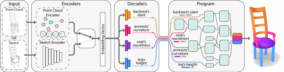
Figure 2: System overview. GeoCode learns to map a point cloud or a sketch input to an intuitively editable parameter space. The input passes through the corresponding encoder to obtain an embedding vector which is then fed to a set of decoders that predict the interpretable parameters. The program enforces a set of rules that, given a parameter representation, produces a high-quality shape by construction.

In this work, we leverage procedural methods to build a program that maps human-interpretable parameters to a high-quality and intuitively editable 3D mesh. In our program, changing a high-level parameter produces a set of low-level instructions which ensure the modified shape is structurally valid. Our human-interpretable parameter space describes a wide range of geometric properties and enables producing broad variations of detailed shapes. Moreover, we design our program to additionally include semantic part labels. Thus, GeoCode contains consistent part segmentation across the generated instances.

To demonstrate the effectiveness of our procedural program, we generate a large dataset with a variety of detailed shapes by sweeping over the interpretable parameter space. Then, we train a neural network to infer the parameter space representation for a point cloud or a sketch as input. Once the input is mapped to the parameter space, and then processed through our program, the resulting shape can be intuitively edited, as seen in Fig. 1. Moreover, we show that shapes can be easily mixed and interpolated using their interpretable parameter representation. We also show that our system generalizes to inputs from different distributions than the training set, such as free-form user-created sketches, sketches generated from images in the wild, noisy point cloud data, real-world point cloud scans, and more.

In summary, we propose a technique for representing shapes using an intuitively editable parameter space. We build a neural network that learns to map a given point cloud or sketch to the parameter space, and our program translates the parameter representation and produces high-quality mesh outputs by construction. The resulting shapes are native to conventional 3D modeling pipelines. We compare our approach against existing techniques and find that GeoCode can more accurately infer and recover 3D shapes. Another notable advantage of GeoCode is its ability to generate physically-plausible objects, which we demonstrate by dropping samples from above a flat plane in a physics simulation. Code and results available: {https://github.com/threedle/GeoCode}.

2 Related Work

Shape reconstruction. Several works used deep learning methods to reconstruct a 3D object from a sketch. Delanoy et al. [6] and Li et al. [23] predict voxel grid and depth with normal maps, respectively, which are then converted to meshes. Another approach is to produce a CAD shape to improve the structural integrity and edit capability of the reconstructed mesh. For example, Sketch2CAD [21] and Free2CAD [22] trained neural networks to parse 2D sketches into sequences of CAD commands, and ComplexGen [10] created CAD shapes using point clouds as input.

While GeoCode also converts sketches and point clouds into 3D editable shapes, the final shapes are fundamentally different from CAD shapes. The final shapes are intuitively controlled by a set of human-interpretable parameters that capture the geometric attributes of different parts of the shape. Changing one parameter results in local changes that can propagate to the rest of the shape to maintain its physical validity. In contrast, CAD objects are composed of low-level operations. Editing one CAD operation changes only a part of the shape, which makes keeping its structural integrity very challenging.

We also note that there is a large body of research on recovering the underlying surface mesh from a point cloud input [14, 19, 20, 11, 26]. Our goal in this paper is different. We aim to produce an intuitively editable mesh version of the point cloud, while surface reconstruction works focus mainly on recovering a holistic 3D shape.

Procedural program. Procedural models are powerful representations of shapes, which have recently gained increasing popularity. Recent works tried to directly infer procedural program instructions to build a shape. For example, PLAD [18], ShapeAssembly [15], and ShapeMOD [16] created instruction languages that can construct 3D shapes by defining cuboids and procedurally attaching them.

While these methods use bounding box primitives to abstract the shape, our program builds an expressive geometry of different parts, which can also be easily modified to manipulate the geometry. Another fundamental difference is that we do not directly infer the program instructions. Instead, we first predict the geometric attributes of the input. Then, these attributes are used by our structurally-designed procedural program to build the output shape.

Another approach for object construction is to learn the hierarchical structure of shape parts and assemble them to create the complete shape [24, 27, 35, 17, 30]. Such models rely on annotated datasets, with fine-grained part labels and given relation graphs [28]. On the contrary, our method operates on holistic sketches or point cloud inputs, and the semantic part information is built-in within our program.

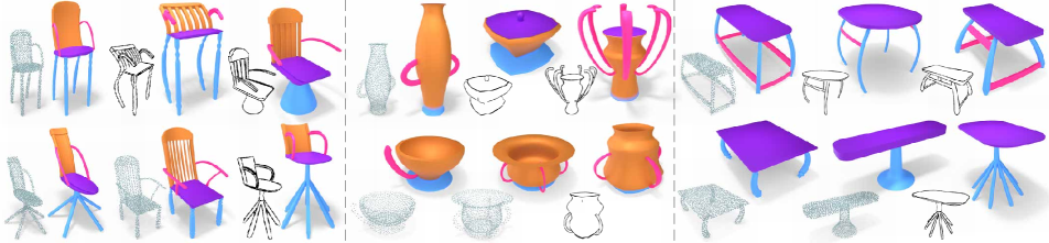
Figure 3: Shape gallery. Showing reconstructed shapes on our test set. Our procedural program produces high-quality geometry from a 3D point cloud or a 2D sketch and contains consistent part segmentation information across the resulting shapes.

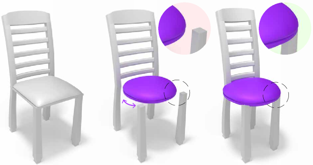
Figure 4: Structural integrity. GeoCode ensures that an edited shape remains structurally plausible. Changing the parameters of the shape (left) to modify the seat in isolation will lead to an undesirable result (middle). Our program (right) properly propagates the edit to the remainder of the shape.

3 Method

Given an input object, represented as a 3D point cloud or a 2D sketch image, our goal is to recover an editable 3D mesh. To do that, we develop a procedural program, which enforces a set of shape rules and is parameterized by human-interpretable controls. We recover an editable 3D shape by training a neural network to infer the set of procedural program parameters and run the program to construct the output shape. An overview is given in Fig. 2.

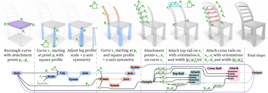
Figure 5: Procedural shape construction. GeoCode generates a set of low-level instructions which adhere to high-level rules to produce a structurally valid shape. In the above figure, we exemplify the inner working of our procedural program. First, we create a seat using its profile and a curve (the latter is not displayed in the figure) and go on the define attachment points on the seat. Note that throughout the graph, colored edges pass mesh as information. In step 2, a leg is generated using the same method and attached to point $\mathbf{p}_{\tt 1}$. In the same step, we apply a Scale along the curve $\mathbf{c}_{\tt 1}$ to make the leg thicker at the bottom, and we duplicated the leg using a symmetry rule (Symm). Lastly, we Join both legs to pass them further as one unit. In step 3, a frame is generated using $\mathbf{c}_{\tt 2}$ and a squared profile with an edge length $\mathbf{w}$, we Join the legs and newly formed frame and apply a symmetry (Symm) to replicate them to the other side of the chair. Step 4 shows how attachment points are created on $\mathbf{c}_{\tt 2}$ by sampling (Sample) it 5 times. At the same time, we also retrieve the normal at each point. In step 5, a previously generated top-rail shape is attached to the top of the frame at point $\mathbf{s}_{\tt 1}$ and we orient it to match the normal $\bar{\mathbf{n}}_{\tt 1}$ at that point. We then scale its width so it is connected seamlessly to both sides of the frame. To obtain the final shape, in step 6, the cross rails are attached at points $\mathbf{s}_{\tt 2}$..$\mathbf{s}_{\tt 5}$ with orientations matching $\bar{\mathbf{n}}_{\tt 2}..\bar{\mathbf{n}}_{\tt 5}$ and a scale that will make them fit between both sides of the frame.

In addition to the intuitive controls, our program includes structural information, which results in a consistent semantic part segmentation by construction. Fig. 3 presents a gallery of our shapes, along with their semantic part segmentation. Moreover, the program keeps the geometrical validity after shape manipulation, as exemplified in Fig. 4.

Below, we elaborate on our procedural program in Sec. 3.1, its input, output, and operation. In Sec. 3.2, we explain the structure of our network which infers the human-interpretable parameters from a point cloud or a sketch input and we explain its training process.

3.1 Interpretable Shape Program

Our program supports three types of human-intuitive input parameters: discrete, binary, and continuous, as exemplified in Fig. 1. The program offers disentangled control over the shape, which enables modification of a specific part while keeping all others intact. However, it also models complex structural interactions, such that one part influences another, and the latter is adapted automatically to preserve part contact and retain the structural integrity of the shape. For example, in Fig. 1, the number of backrest slats is increased while the rest of the chair remains the same. In contrast, replacing the square seat with a round one in Fig. 4 makes the seat narrower, which also changes the leg’s position and decreases the width of the backrest accordingly.

The program is implemented as a directed acyclic graph (DAG) comprised of operation nodes and edges. The operation nodes can hold anything from a single value, all the way to complex geometry. Examples of operation nodes include math operations or vector operations; mesh primitives, such as cubes or spheres; line primitives such as a Bezier curve; and rigid transformation (translation, rotation, and scale).

A collection of operations is responsible to generate a shape element and one or several shape elements build a shape part. For example, the armrest of a chair is considered a part that is comprised of up to three shape elements: an arm, an arm support, and an arm cushion. Parts are attached together and replicated using symmetry rules to create the final shape. We refer our reader to Fig. 5 for an inside look at how our program is built.

Selected operation nodes are parameterized by the input parameters, allowing the user to interact with the program and control the resulting shape. The operations are chained together, receive, process and then pass the information along their edges, and model shape elements and inter-part influences. The program has a single final node, which outputs a mesh.

We group operation nodes into collections that make up a single semantic part in the final shape. For example, the backrest, seat, armrests, and legs of a chair, all have their own operation-node collections. This design choice results in segmented parts by construction, as shown in Fig. 3. The operation-node collections also pass information between each other, which keeps the structural integrity of the shape during edits. This property is demonstrated in Fig. 4.

Construction of shape elements. In most cases, we model a shape element using curves. In other cases, we use mesh primitives such as a sphere or a plane that we modify to our needs. A curve-based shape element is built out of two curves: a one-dimensional curve $\mathbf{c}_{\tt 1}$, which describes a path in the 3D space, and a two-dimensional curve $\mathbf{c}_{\tt 2}$, which describes the profile of the shape. The profile $\mathbf{c}_{\tt 2}$ is extruded along the path that $\mathbf{c}_{\tt 1}$ defines, a process that creates the shape element’s 3D mesh.

Controlling the appearance of the shape element is done by setting the scale of the profile $\mathbf{c}_{\tt 2}$ at each point along the curve $\mathbf{c}_{\tt 1}$. An example of this process is presented in the second step in Fig. 5. Another way to alter the appearance of a shape element is to change the profile $\mathbf{c}_{\tt 2}$ itself. Examples of such edits are changing the roundness of the seat of a chair (Fig. 1) or interpolating the body of a vase between the circle and square profiles (Fig. 10).

Structural relations. A notable benefit of cultivating curves to build shape elements is the ease of defining attachment points on a curve, by setting points with relative distance along the curve. Meaning, given a shape element $\mathcal{A}$, which is built from a curve $\mathbf{c}_{\tt 1}$ and a profile $\mathbf{c}_{\tt 2}$, an attachment point $\mathbf{p}_{\tt 1}$ on the shape element is defined by a single float number $\mathbf{p}_{\tt 1}\in[0,1]$. A value of $0.0$ is the start point of the curve $\mathbf{c}_{\tt 1}$, while a value of $1.0$ is the end point of the same curve. We attach a shape element $\mathcal{B}$ to shape element $\mathcal{A}$ by defining an attachment point on each one. We optionally set the orientation of $\mathcal{B}$ to match the normal of $\mathbf{c}_{\tt 1}$ at the attachment point $\mathbf{p}_{\tt 1}$. Steps 5 and 6 in Fig. 5 show the placement of a top rail and the cross-rails for a chair in this manner. Scaling shape elements is achieved by calculating distances between attachment points.

Other structural relations do not require attachment points and rely simply on symmetry. This is shown in steps 2 and 3 in Fig. 5, where we use symmetry to replicate the legs of the chair and the frame. We also employ rotational symmetry, for example, chairs with swivel legs and vases that have multiple handles in (Fig. 3).

Edits. The input to our program is a set of human-interpretable parameters. These can set the structure of the shape (e.g., the height of a chair’s seat or the points where the handles will be attached to a vase) or modify shape elements’ appearance (e.g., the width of a leg or the roundness of the seat of a chair). Structural edits affect the one-dimensional curves (e.g., $\mathbf{c}_{\tt 1}$) and propagate to other shape elements using the attachment points and symmetries that are enforced by our program.

Edits to the appearance of shape elements affect the two-dimensional curves (e.g., $\mathbf{c}_{\tt 2}$) and can cause structural edits as well. An example of this case is increasing the seat’s roundness, which causes the chair to get narrower by imposing structural edits on the shape that bring the legs and the frame of the chair closer together. Considering the opposite direction, edits to the structure of the shape cannot affect the appearance of any of the shape elements. For example, changing the height of the seat of the chair will not affect the seat’s roundness or the appearance of the legs.

Part visibility. In our program, we include support for binary properties, e.g., a chair may or may not include armrests. As part of the probability distribution function for our human-interpretable parameter, we add a part existence label to parameters that control a switchable part of the shape.

Continuing the armrests example, all the parameters that control the shape of the armrests may have no effect on the final chair shape if the binary parameter controlling the visibility of the armrests is set to false, and hence, the final chair shape will not include them. Consequently, these parameters will be given the option to be set to that part existence label. A pre-processing stage on our datasets assigns any such parameter to the part existence label if the part it controls is not visible in the final shape. This step is done based on a set of visibility rules that are a part of our program.

3.2 Mapping to the Program Space

To map a point cloud or sketch input to the human-interpretable parameter representation, we employ an encoder-decoder network architecture. The encoder embeds the input into a global feature vector. Then, we use a set of decoders where each one translates the embedding vector to a single parameter. Together, the final interpretable representation is obtained. Finally, we run the program and recover the 3D shape. Fig. 2 illustrates our system design.

Problem formulation. We formulate the shape recovery problem as predicting the human-interpretable parameters from a given point cloud or sketch. Let us denote the program parameters as $\{p_{i}\}$, where each parameter can take $N_{i}$ discrete values. Continuous program parameters, such as thickness or height, are discretized uniformly over their range. The ground-truth value of the parameter is encoded by a one-hot vector $\mathbf{y}_{i}\in\{0,1\}^{N_{i}}$. The ground-truth representation for all the parameters is the concatenation of all $\{\mathbf{y}_{i}\}$, which we denote as $\mathbf{y}\in\{0,1\}^{\sum_{i}\!N_{i}}$.

The prediction of the program parameters by the network is done as follows:

$$\hat{\mathbf{y}}_{\tt pc}=\mathbf{D}(\mathbf{E}_{\tt pc}(\mathbf{c})),~{}~{}~{}\hat{\mathbf{y}}_{\tt sketch}=\mathbf{D}(\mathbf{E}_{\tt sketch}(\mathbf{s})),$$ (1)

where $\hat{\mathbf{y}}_{pc}$ and $\hat{\mathbf{y}}_{sketch}$ are the predicted parameters in one-hot representation from the point cloud $\mathbf{c}$ or sketch $\mathbf{s}$, respectively, $\mathbf{E}_{\tt pc}$ is the point cloud encoder and $\mathbf{E}_{\tt sketch}$ is the sketch encoder, and $\mathbf{D}$ denotes the shared decoders.

To train the network, we use our program and construct a dataset of point cloud, sketch, and ground-truth triplets, i.e., $\mathcal{D}=\{(\mathbf{c},\mathbf{s},\mathbf{y})\}$. Then, we train the network with the loss function:

$$\mathcal{L}=\frac{1}{|\mathcal{D}|}\sum_{(\mathbf{c},\mathbf{s},\mathbf{y})\in\mathcal{D}}\text{CE}(\hat{\mathbf{y}}_{\tt pc},\mathbf{y})+\text{CE}(\hat{\mathbf{y}}_{\tt sketch},\mathbf{y}),$$ (2)

where CE denotes the sum of cross-entropy losses over each one-hot vector $\mathbf{y}_{i}$.

4 Experiments

We present qualitative and quantitative evaluations of our method’s performance on shape recovery and editing. We demonstrate GeoCode’s ability to recover 3D shapes from point clouds and sketches from the held-out test set of our dataset and form shapes in the wild and contrast it with alternative procedural shape reconstruction methods [27, 15]. Furthermore, we show that our system provides editing capabilities on the reconstructed shapes, such as modifying the geometry of a part, mixing two shapes, and interpolating between two shapes. Finally, we demonstrate GeoCode’s robustness against various input perturbations.

Dataset	Stable GT Samples	Stable PC Predictions	Stable Sketch Predictions
Chair	91.01%	90.28%	91.54%
Vase	100.00%	99.79%	99.57%
Table	99.84%	96.33%	97.24%

Table 1: Structural stability. We show the percentage of ground truth and predicted samples from our test set that are structurally stable according to our stability metric. We show a high percentage of ground truth sample stability and matching high percentages for our predicted shapes.

Dataset and implementation details. To train and evaluate our system, we generated train, validation, and test datasets using our shape program. For each generated 3D shape, we sample 1,500 points using Farthest Point Sampling [7] and an additional 800 randomly sampled points. We render the 2D sketch images using Blender’s [4] stroke-bases rendering engine Freestyle [8] from three camera angles while training only on two of them. Sketches are randomly augmented using horizontal flip, stroke dilation, and stroke erosion. We have control over the sampling granularity of each continuous parameter, as well as how many random shapes are generated for each possible value of each parameter. During the dataset generation, we make sure that no two shapes are the same. We design three programs that we built using Blender [4] Geometry Nodes [9], each one handling a different shape domain of chairs, vases, and tables, and have 59, 39, and 36 human-interpretable parameters as input, respectively. In total, the train set for each domain contains 9,570 chairs, 9,330 vases, and 6,270 tables. The validation and test sets each contain 957 chairs, 933 vases, and 627 tables.

For the point cloud encoder, we use Dynamic Graph CNN (DGCNN) [37] and employ the VGG architecture [32] for the sketch encoder. The decoder utilizes a multi-layer perceptron with three layers for each program parameter. Since each human-interpretable parameter may have a different number of values, the output layer size of each decoder varies according to the number of possible classes of the parameter the decoder is responsible for.

Method / Category	Chairs $\downarrow$	Vases $\downarrow$
StructureNet [27]	0.0203	0.0215
ShapeAssembly [15]	0.0134	-
GeoCode (ours)	0.0062	0.0112

Table 2: Reconstruction comparison for the COSEG dataset. GeoCode achieves significantly lower Chamfer Distance on both the evaluated domains of chairs and vases.

4.1 Shape Recovery

We evaluate our method’s ability to recover 3D shapes from samples in our test set. We also consider out-of-distribution examples, including shapes from COSEG [36], real-world scan-based datasets such as ScanNet [5], hand-drawn sketches, and sketches generated by CLIPasso [34] from images in the wild.

Baselines and evaluation metric. We compare our method against two structure-aware baselines, StructureNet [27] and ShapeAssembly [15]. The decoders of both these models work in conjunction with a point cloud encoder to reconstruct shapes from unannotated point clouds. As instructed by the authors, we train a point cloud encoder [31] on the PartNet dataset [28] to map point clouds to the StructureNet and to the ShapeAssembly latent spaces. During inference, we use the trained encoder with the decoders released by the authors to reconstruct shapes from point clouds sampled from COSEG shapes [36].

For quantitative evaluations, we use the bi-directional Chamfer Distance [1], defined as the average minimum distance of each point in one shape to a point in the other shape and vice versa. The Chamfer Distance is calculated using 10,000 randomly sampled points on the ground truth and reconstructed shapes.

Results on our dataset. We first verify qualitatively that our system can correctly reconstruct shapes given an input point cloud or sketch. In Fig. 3, we show examples of reconstructed shapes and their corresponding inputs. The reconstructions are visually similar to the input point clouds and sketches, confirming that our system can faithfully recover shapes for inputs that are within our data distribution.

Structural stability. During dataset generation we take measures to make sure our samples are structurally stable. For instance, the vases could have a base that is too narrow and will make them tip over under their own weight in real life. During inference time, we do not enforce any stability-inducing modification on our predictions. To ensure that our predictions are structurally stable, we define a binary stability metric. We consider a shape to be stable if it has no parts that are detached, and it remains standing in a physics simulation after a drop onto a flat plane from a height of 5% of the shape’s height. In Tab. 1, we can see that GeoCode’s ground truth shapes are mostly stable. Moreover, the predictions our system generates are on par with the ground-truth data in terms of their stability.

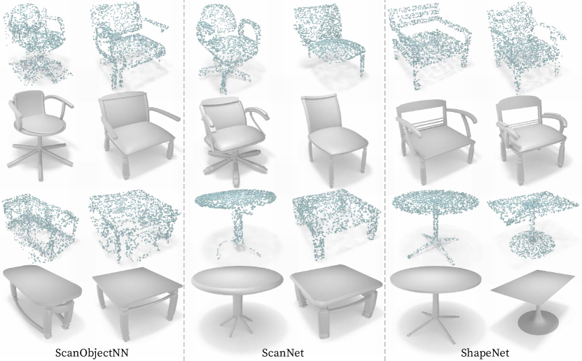
Figure 6: Generalization to out-of-distribution point clouds. We show reconstruction results of GeoCode for point cloud from various datasets. We use scanned objects from ScanObjectNN [33] and ScanNet [5] and also test on point clouds from ShapeNet [2]. Our method outputs plausible reconstructions, despite hindered point cloud quality that is characterized by noise and missing parts.

Comparison on the COSEG dataset. Next, we evaluate the generalization power of GeoCode beyond our generated data distribution and compare our reconstruction performance with previous works [27, 15]. For this experiment, we use the COSEG [36] chair and vase shape sets of 400 chairs and 300 vases. Neither we nor the baseline methods have been trained on this dataset, so we find it a fair test for the generalization ability.

From each shape, we create point clouds with 1,500 points that are sampled using Farthest Point Sampling [7] and additional 800 randomly sampled points. Tab. 2 shows the average Chamfer Distance for the chair and vase sets from COSEG for different reconstruction methods. We observe that our system produces more accurate reconstructions than the baselines. Visual comparison results are presented in the supplementary.

Reconstruction from out-of-distribution shapes. To further demonstrate the generalization capability of GeoCode, we choose three known 3D shape datasets and reconstruct shapes from these datasets for point cloud inputs. First, we consider two real-world scan-based datasets, ScanObjectNN [33] and ScanNet [5], which include LiDAR scans of objects and scenes, respectively. For ScanObjectNN, we use the point clouds from the main dataset. For ScanNet, we extract objects from the scene using the provided segmentation masks and randomly sample point clouds from them. We also consider ShapeNet [2] and produce point clouds by randomly sampling its shapes. For all the datasets, we end up with point clouds having 2,048 points.

In Fig. 6 we show the reconstruction for two domains, chairs, and tables. Our method is able to recover shapes that capture the main geometric features of the out-of-distribution samples. Moreover, point clouds produced from scanned objects are contaminated by noise and partiality. Still, GeoCode is able to produce compelling results in these cases as well.

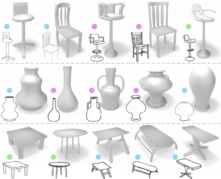
Figure 7: Hand drawn sketches. We show the ability of GeoCode to recover an editable 3D shape from free-form sketches, sketch outlining, and sketches in-the-wild. Our system produces a 3D shape that captures the main attributes of the input sketches.

Figure 8: Sketches from images. Starting with an input image, we automatically create a sketch using CLIPasso [34]. Our method generates editable shapes that closely match the original images and corresponding sketches that have a variety of styles.

Reconstruction from hand-drawn sketches. Fig. 7 shows reconstruction examples from free-form, outlined, and in-the-wild sketches. Our system is able to generalize and capture the main features from the sketches and produce shapes that are visually similar to the input sketches. These sketches possess different styles and are drawn from different angles compared to the sketches we trained on.

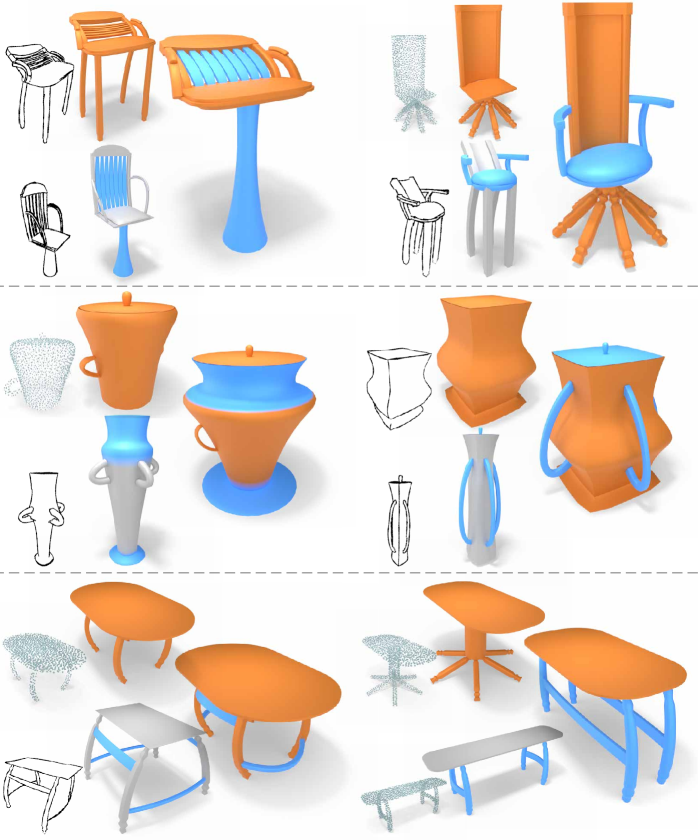
Figure 9: Shape mixing. Although mixing can be done using a larger number of shapes, we demonstrate it by taking a source shape and choosing geometric features from a second shape. GeoCode will either add the selected geometric features to the source shape (e.g. handles are added to the second vase), or it will override them in the source shape (e.g. cross rails in the backrest of the first chair are replaced with vertical rails). In both cases, the structural integrity of the shape is maintained.

Reconstruction from CLIPasso sketches. Fig. 8 shows reconstruction examples from sketches generated by CLIPasso [34]. We use CLIPasso to convert images of chairs, vases, and tables found in the wild to sketches with various numbers of strokes. The sketches produced by CLIPasso are noisy and often contain artifacts, these make them visually different from sketches found in our datasets. We observe that, overall, the shapes reconstructed from our system are sensible and correctly recover features from the shapes in the original images. This suggests that our network is able to express shapes with human-interpretable parameters given an out-of-distribution input.

4.2 Shape Editing

Beyond shape recovery, we show that our interpretable parameter space allows for easy shape editing. This property is exemplified by shape mixing and shape interpolation.

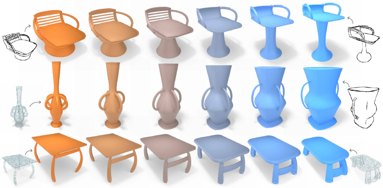
Figure 10: Shape interpolation. We uniformly interpolate between two (left and right) GeoCode shapes. Interpolations contain gradual changes (continuous parameters) as well as sharp structural changes (discrete or binary parameters).

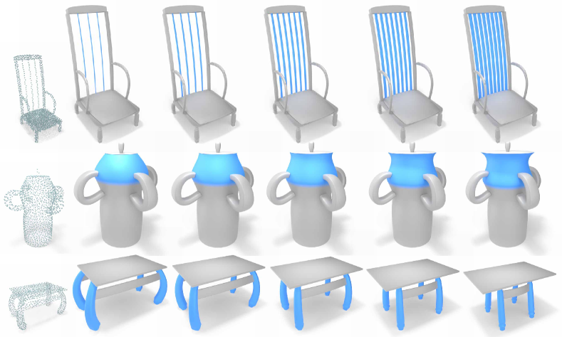
Figure 11: Selective editing. GeoCode enables controlled editing over a particular attribute, while accurately adapting the remaining parts of the shape. Note the vase handles remain connected after each gradual edit.

Shape mixing. We show that our system can mix shapes by selecting a set of parameters from the human-interpretable parameter space representation of source shapes and combining them to form a representation that produces the final shape. When mixing disjointed parts, such as handles from one shape and legs from another, it is guaranteed that the mixed shape will capture the selected parts from the corresponding source shapes and transfer them to the resulting shape. Fig. 9 shows mixing examples between pairs of shapes reconstructed from point clouds and sketches. The resulting shapes are based on the first shape with the addition of selected parts from a second shape. The final mixed shape is structurally valid and physically plausible.

Shape Interpolation. GeoCode is effective in interpolating between shapes and interpolating between selected parts of the shapes. Fig. 10 shows interpolation between pairs of shapes reconstructed from point clouds and sketches where we interpolate across all the parameters for $\alpha\in[0,1]$ in 0.2 increments. Fig. 11 shows interpolation over selected geometric features for $\alpha\in[0,1]$ in 0.25 increments.

Dataset	Input	$\sim$25K Faces $\downarrow$	$\sim$2K Faces $\downarrow$	$\sim$120 Faces $\downarrow$
Chair	PC	0.0004	0.00041	0.00133
	Sketch	0.00106	0.00117	0.00227
Vase	PC	0.00264	0.0028	0.00613
	Sketch	0.00488	0.00517	0.0116

Table 3: Reconstruction from simplified shapes. Comparing the average Chamfer Distance on our test set at different mesh simplification factors. The averages only slightly increase for a simplification factor of $10\times$ ($\sim$2K faces) compared to the original mesh ($\sim$25K faces) and increase more drastically for a high simplification factor of $100\times$ ($\sim$120 faces).

4.3 Robustness

In this section, we evaluate our method’s robustness to slightly deformed inputs. Specifically, we both qualitatively and quantitatively evaluate the performance of GeoCode on the following deformation: sketches of simplified shapes and point clouds sampled from simplified shapes. For other deformation/perturbation including sketches rendered from novel angles, random point clouds with decreasing number of points, and point clouds with added Gaussian noise, we refer the reader to the supplemental.

Reconstruction from simplified shapes. Simplification reduces the number of polygons and, therefore, the level of detail in the shape. In this experiment, we show that our system is able to reconstruct shapes from both point cloud and sketch inputs that are produced from simplified meshes. We compare the non-simplified reconstruction where we have approximately 25K faces (this number varies depending on the visible parts in the shape) to simplified versions where the average number of faces is decreased by a factor of $10\times$ ($\sim$2K faces), and a factor of $100\times$ ($\sim$120 faces).

Tab. 3 shows the average Chamfer Distance between the predictions from the point cloud or sketch inputs that were produced from the simplified shape and the non-simplified original ground-truth shape. It is evident that our method is robust to simplification with a factor of $10\times$ and performs slightly worst for a simplification factor of $100\times$. We refer the reader to the supplementary for qualitative results that visualize the simplified shapes and their reconstructions.

5 Conclusions and Future Work

In this paper, we presented GeoCode, a novel method that represents shapes using a human-interpretable parameter space. We achieved this by building a procedural program controlled by the intuitive parameter space and training a neural network to predict the parameter representation for an input point cloud or sketch. We showed that our system produces structurally valid 3D geometry and enables editing of the resulting shape easily and intuitively. We also demonstrated that GeoCode generalized well to out-of-distribution point clouds and sketches in the wild.

In the future, we are interested in incorporating additional attributes into our procedural program to include UV texture maps and material properties for the resulting shapes. Another venue we aim to explore is extending our method for representing 3D scenes.

6 Acknowledgments

We thank the University of Chicago for providing the AI cluster resources, services, and the professional support of the technical staff. This work was also supported in part by gifts from Adobe Research. Finally, we would like to thank R. Kenny Jones, Chen Dudai, and the members of 3DL for their thorough and insightful feedback on our work.

Supplementary Material for GeoCode: Interpretable Shape Programs

We provide additional information about GeoCode. Appendix A describes two complementary videos for our method and shows additional results for experiments presented in the paper. In Appendix B, we report additional experiments, evaluating the robustness of GeoCode. Lastly, Appendix C elaborates on our implementation details, including our dataset creation, network architecture, and training scheme.

Appendix A Additional Results

A.1 Complementary Videos

Demo video. As part of the supplementary, we provide a video (GeoCode Demo.mp4) showing the variety of shapes that our method can produce. In addition, the video will help the reader understand the ease of controllability that the method provides, as well as show how the structural integrity is maintained continuously while editing the shapes.

For a short length at the beginning of the video, we also show the ease at which shapes can be changed using human-interpretable parameters, by showing the shape along with the actual values of selected parameters of the chair:

• Cross Rail Count (discrete) - controls the number of cross rails appearing on the backrest of the chair.

• Armrest (boolean) - toggles the existence of the armrests, when set to True the armrests will appear while maintaining the structural integrity of the current chair shape.

• Armrest Height (continuous) - controls the attachment point of the base of the armrests to the backrest of the chair. Higher values, mean the armrests are connected to the frame at a higher position. The value is treated as a percentage of the height of the frame, for example, a value of 0.5 will place the armrests at an equal height between the seat and the top of the frame.

• Seat Roundness (continuous) - controls the shape of the seat. The higher this value is, the more rounded the seat shape will be. The video helps to show that the entire chair is adjusted automatically to fit the changing seat shape and maintain the structural integrity of the chair. We show how this is achieved when we describe our method in Fig. 5 of the main paper.

• Seat Height (continuous) - controls the height of the seat. The legs, the frame, and other components of the chair, like the cross rail, are all adjusted automatically to fit the seat position in a continuous manner.

• Backrest Curvature (continuous) - this parameter controls how rounded the cross rails and top rail are. A value of 0.0 means that the backrest is completely flat, while higher values will make the backrest appear more rounded. In reality, it also controls other components that are not shown in the video, like the vertical rails.

• Backrest Slant (continuous) - allows adjusting how slanted the backrest is. A value of 0.0 means the backrest is perpendicular to the ground (or equivalently, to the seat), while higher values make the backrest lean backward in a rounded fashion.

Simulation demostration. As explained in Sec. 4 of the main paper, our structural stability metric checks that a given shape is structurally valid by testing two things, checking for the existence of loose parts, and dropping the shape from a height onto a flat plane and testing that the height of the shape has not changed after the drop. In the attached video (GeoCode Simulation.mp4) we show 15 samples tested in that simulation, from all three domains, chair, vase, and table. The drop height was increased for the purpose of visual demonstration, from the 5% that we used when creating Tab. 1 to 20% of the shape’s longest dimension.

A.2 Visual Comparison on the COSEG Dataset

We present qualitative results that complement Tab. 2 shown in the main paper. In this experiment, we evaluated GeoCode on the shape recovery task while comparing to the works [27, 15] using COSEG [36] chair and vase shape sets.

The qualitative results in Fig. 12 show the generalization power of GeoCode while also explaining the drastic decrease in average Chamfer Distance compared to the other two methods. GeoCode can more accurately capture geometric features of the ground-truth shapes when compared to both StructureNet [27] and ShapeAssembly [15].

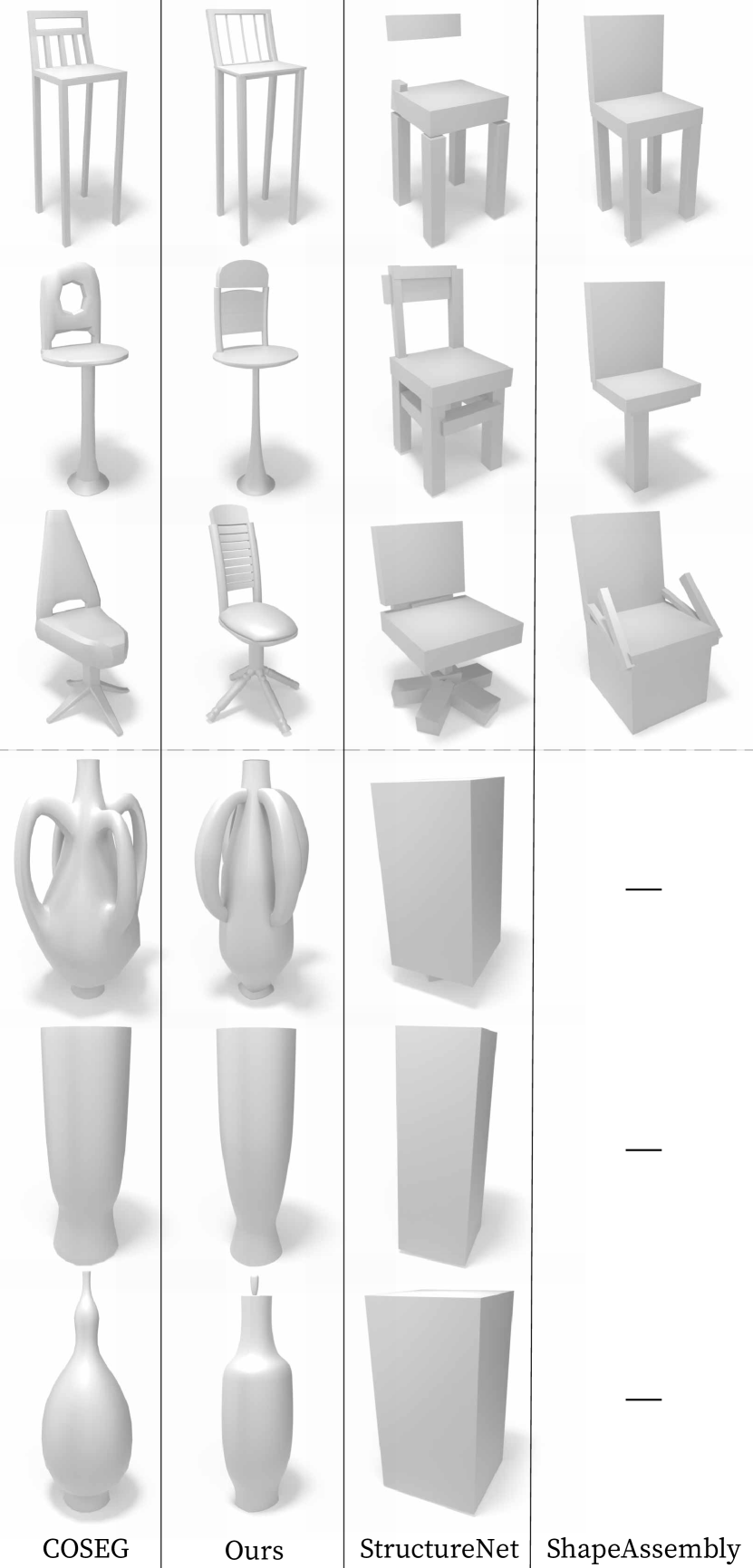
Figure 12: Visual Comparison on the COSEG Dataset. We show the reconstruction results of GeoCode, StructureNet [27], and ShapeAssembly [15] on point cloud inputs generated from COSEG [36] samples. The compared methods yield crude approximations of the input geometry and may output a shape with detached parts. In contrast, GeoCode’s predictions are much closer to the original shape while also being structurally sound.

Appendix B Additional Experiments

B.1 Shape Recovery

Reconstruction from point cloud vs. sketch. We study the reconstruction performance of both point cloud and sketch inputs on our test sets for all three domains. Note that the calculation of the average Chamfer Distance for the sketch input type was done using only the camera angles that were seen during training.

In Tab. 4 we see that, overall, reconstruction from point clouds generally performs better compared to reconstruction from sketch inputs. For example,  Tab. 4 shows that for the chair domain, the average Chamfer Distance when reconstructing from point clouds is 2.5 times better compared to reconstruction from sketches. The vase and table domains show similar results. We attribute this, in part, to the fact that the scale of the shape cannot be effectively captured from a single image, while a point cloud inherently encodes the scale of the shape. The qualitative results for this experiment are shown in Fig. 13.

Figure 13: Reconstruction from point cloud vs. sketch. We compare the reconstruction results of GeoCode from point clouds and sketches. The Chamfer Distance for each prediction is noted near the reconstruction result. In most cases, point cloud reconstruction yields a better result. However, sketch reconstruction may sometimes perform better (first vase and first table).

Dataset	Point Cloud	Sketch
Chair	0.0004	0.00106
Vase	0.00264	0.00488
Table	0.00044	0.0025

Table 4: Reconstruction from point cloud vs. sketch. Showing the average Chamfer Distance for the reconstruction task on our test set. We compare the reconstruction results of the point cloud and sketch inputs. Note that when calculating the average Chamfer Distance for sketch input, we only consider sketches from camera angles that we trained on. Point cloud reconstruction performs better in all three domains. The chair domain is the best performer out of the three.

B.2 Robustness

Reconstruction from simplified shapes. We complement our quantitative results shown in Tab. 3 of the main paper with qualitative results. Additionally, we provide the quantitative results for the table domain. Tab. 5 shows the average Chamfer Distance for the table domain. Similarly to the other domains, both point cloud and sketch reconstruction experience only a slight increase in the Chamfer Distance for the lower simplification factor of $\times 10$ ($\sim$2K faces). However, a drastic increase in Chamfer Distance is registered for both input types at the higher simplification factor $\times 100$ ($\sim$120 faces). We show the qualitative results for this experiment in Fig. 14.

Dataset	Input	$\sim$25K Faces $\downarrow$	$\sim$2K Faces $\downarrow$	$\sim$120 Faces $\downarrow$
Table	PC	0.00043	0.00044	0.00149
	Sketch	0.00222	0.00308	0.0052

Table 5: Reconstruction from simplified shapes. Complementing Tab. 3 from the main paper with the table domain. We compare the average Chamfer Distance on our test set at different mesh simplification factors. Both point cloud and sketch reconstructions behave similarly to the chair and vase domains. The averages only slightly increase for the lower simplification factor of $10\times$ ($\sim$2K faces) compared to the original shape ($\sim$25K faces) but register a drastic increase for the higher simplification factor of $100\times$ ($\sim$120 faces).

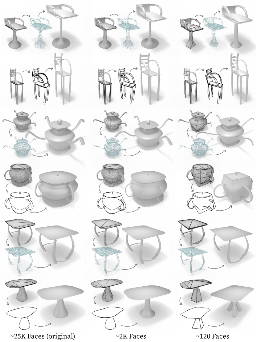
Figure 14: Reconstruction from simplified shapes. We perturb the test set via mesh simplification and show the reconstruction for point clouds and sketches. From left to right: the original shapes with no simplification ($\sim$25K faces), simplification factor of $\times 10$ ($\sim$2K faces), followed by a simplification factor of $\times 100$ ($\sim$120 faces). We observe that GeoCode can still accurately recover the original shape, even when introducing modifications from simplified meshes. Noticeable artifacts appear for the chair reconstruction from the point cloud, particularly the leg of the chair lacks a solid base. Another example is the vase reconstruction from the sketch, where the handles are less accurate, and perhaps understandably, the vase assumes a more square appearance. Also, notice that the leg of the second table is simplified in such a way that is later confused with a swivel leg with three split legs that stem from the base of the tabletop.

Reconstruction from randomly sampled point clouds. Our point clouds during training and testing contain 1,500 points sampled using Farthest Point Sampling [7] and an additional 800 randomly sampled points. In this experiment, we test the robustness of reconstruction performance when the system is given a decreasing number of exclusively randomly sampled points. For each shape in our test set, we randomly sample point clouds with 2,048, 1,024, and 512 points. We then perform reconstructions from these point clouds and compute the average Chamfer Distance between the reconstructed and ground-truth shapes.

Tab. 6 shows that reconstruction from a decreasing number of randomly sampled points increases the average Chamfer Distance between the reconstruction and the ground truth. However, the recon results are still visually similar to ground truth, as evident in Fig. 15. In the last decrement, with only 512 points, our system produces shapes that resemble the overall structure of the ground truth, however, some details are captured with degraded accuracy.

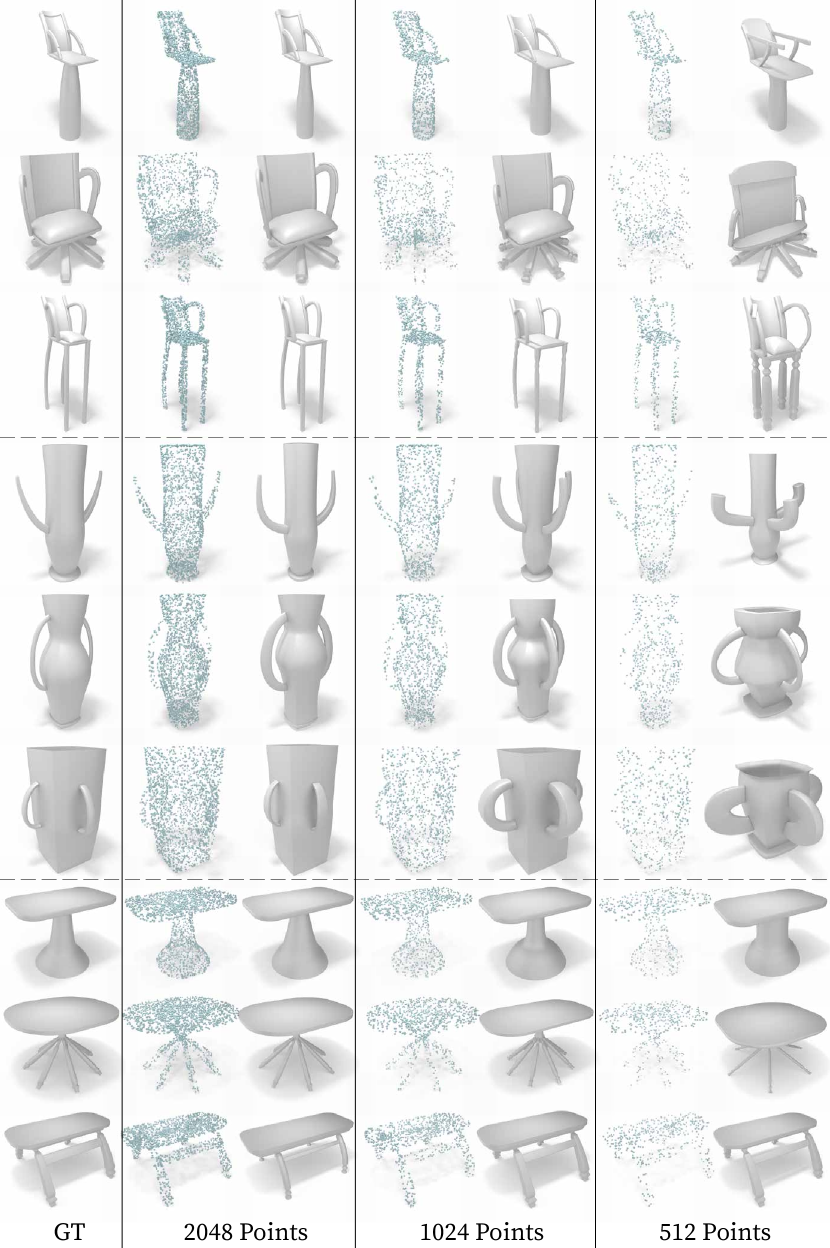
Figure 15: Reconstruction from randomly sampled point clouds. We use random sampling with a progressively decreasing number of points. At 2048 points, GeoCode produces accurate reconstructions. A minor degradation in the level of detail appears for 1024 points, e.g., the second vase’s body is slightly different compared to the ground truth. Lastly, at only 512 points, more considerable reconstruction inaccuracies start to appear. An example of this is seen in the first and last vases, where the body and handles are less accurate. Another example is the second chair, where the seat height, top rail, and armrests are inaccurate.

Dataset	2048	1024	512
Chair	0.00062	0.00311	0.01972
Vase	0.00361	0.0077	0.01914
Table	0.00053	0.00135	0.00536

Table 6: Reconstruction from randomly sampled point clouds. We report the average Chamfer Distance between reconstructed and ground-truth shapes on our test set when reconstructing from randomly sampled point clouds with a varying number of points. Using 2048 points only slightly increases the average Chamfer Distances for all domains when compared to the 1500 Farthest Point Sampling in addition to 800 randomly sampled points that were used in Tab. 4. Decreasing the number of points further to 1024, and then to 512, has a significant effect on the results. However, as shown in Fig. 15, the reconstructions are performing well at 1024 points and suffer inaccuracies mostly at 512 points.

Reconstruction from point clouds with Gaussian noise. To further examine the robustness of our method we add varying levels of Gaussian noise to the point clouds in our test set and evaluate the reconstruction both qualitatively and quantitatively. We consider Gaussian noise with 0 mean and a progressively increasing standard deviation of 0.5%, 1.0%, and 2.5% of the overall size of the shape, corresponding to $\sigma=0.01,0.02$, and $0.05$.

Tab. 7 shows that our method remains somewhat resilient up to $\sigma=0.02$, and begins to struggle when the noise level increases to $\sigma=0.05$. The qualitative analysis in Fig. 16 is consistent with this result.

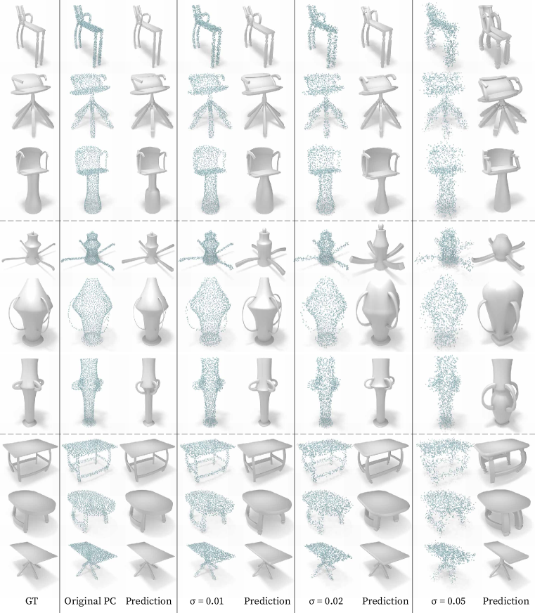
Figure 16: Reconstruction from point clouds with Gaussian noise. Qualitative comparison of the reconstruction from point clouds with varying levels of Gaussian noise with 0 mean and standard deviations of $\sigma=0.01,0.02$, and $0.05$. Taking the first chair and the last vase as examples, we can see that our method produces a rather accurate prediction for both at $\sigma=0.02$, but the reconstructed shapes for $\sigma=0.05$ have less resemblance to the original shape. The first chair and the first table are examples that show an expected property, where the shapes reconstructed from the noisy point cloud tend to appear thicker overall.

Dataset	No Noise	$\sigma=0.01$	$\sigma=0.02$	$\sigma=0.05$
Chair	0.0004	0.0007	0.00125	0.00534
Vase	0.00264	0.00346	0.00492	0.01116
Table	0.00044	0.00076	0.00155	0.00577

Table 7: Reconstruction from point clouds with Gaussian noise. We detail the average Chamfer Distance on our test set when reconstructing from point clouds with various noise levels. Our method is resilient to Gaussian noise when the standard deviation is 0.01, and experiences inaccuracies when more noise is added.

Reconstruction from sketches of various camera angles. We compare the reconstruction from sketches rendered from three different angles. During training, our system sees two of the angles while we leave the third novel angle unseen. For each shape in our test set, we render sketches from all three angles and perform reconstructions from these sketch images.  Tab. 8 shows that the average Chamfer Distance between reconstructed and ground-truth shapes is similar when we reconstruct from the two sketch angles that we trained on. However, reconstructing from the novel angle results in a larger Chamfer Distance.  Fig. 17 shows that the shapes reconstructed from the novel angle are still visually close to the ground truth.

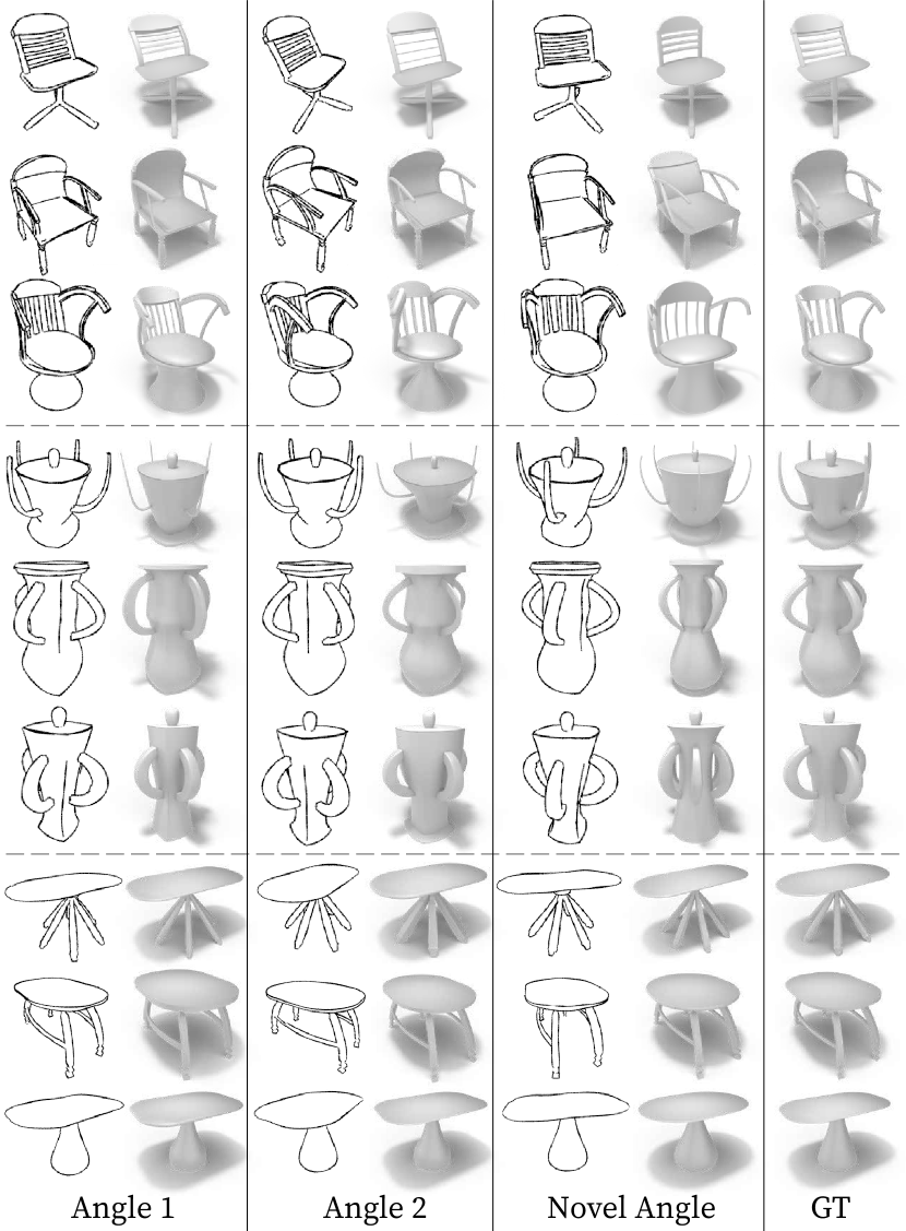
Figure 17: Reconstruction from sketches of various camera angles. Comparison between reconstruction from sketches rendered at different camera angles. The novel angle is an angle that was never seen during training. The two first angles perform similarly with accurate results, while the novel angle produces less accurate results. For example, in the second chair, the backrest is slanted backward for the reconstruction from the novel angle. However, the ground-truth shape and the predictions from the first two angles show a forward-slanted backrest. Another example is the second vase, where the body is noticeably thinner.

Dataset	Angle 1	Angle 2	Novel angle
Chair	0.00108	0.00103	0.00807
Vase	0.00484	0.00491	0.00979
Table	0.00246	0.00254	0.00853

Table 8: Reconstruction from sketches of various camera angles. We provide the average Chamfer Distance between reconstructed and ground-truth shapes in our test set for sketch inputs, comparing the result on sketches generated from the two camera angles that were seen during training with a novel angle unseen during training. The first two angles perform similarly. However, the average Chamfer Distance for the novel angle is increased significantly. Another observation is that the increase in the novel angle is not as pronounced for the vase domain since the vases tend to have rotational symmetry.

B.3 Ablation Study

Classification vs. regression. In our work we supported discrete, boolean, and continuous parameters. We explained in Sec. 3 that continuous parameters are discretized and that the loss function is cross-entropy. In this ablation experiment, we test the performance of reconstruction in terms of average Chamfer Distance while comparing the use of classification vs. regression for the continuous parameters.

To make a fair comparison we also incorporate the existence lable that we discuss in the main paper in Sec. 3. To achieve that, each decoder of a continuous parameter that controls a part of the shape that can be invisible will output two elements instead of one. The first element will be the predicted value of the parameter, while the second element predicts the existence label. Whenever the prediction of the second element exceeds 0.5 we say that the actual predicted value is the existence label. During loss calculation, we accumulate the Mean Square Error of both elements. If the existence label was predicted (the second element is greater than 0.5) then we avoid collecting the regression loss of the first element (which predicts the value of the parameter). In Tab. 9 we can see that using classification for all the parameters yields better average Chamfer Distance results.

Method	Point Cloud $\downarrow$	Sketch $\downarrow$
Classification	0.0004	0.00106
Regression	0.00198	0.00364

Table 9: Classification vs. regression. We train the chair network in two different ways. Classification: continuous parameters are discretized and the loss function is cross-entropy, as described in Sec. 3. Regression: we employ cross-entropy loss for discrete and binary parameters, but we use regression to predict continuous ones. Note that we also use the existence label for the regression parameters to make a fair comparison. We can see that the Chamfer Distance is better overall when using classification loss for all the parameters.

Joint training vs. separate training. In this experiment we wish to find out whether training separately improves the average Chamfer Distance for recovered shapes. We train the network as two separate networks, one for point cloud inputs and another for sketch inputs. To begin with, the encoders (point cloud encoder and sketch encoder) are already separated, but we have to duplicate the decoders in such a way that both networks now have their own decoding network. We note that this effectively doubles the number of weights in the decoding part of each separate network.

Method	Point Cloud $\downarrow$	Sketch $\downarrow$
Jointly	0.0004	0.00106
Separately	0.00037	0.00098

Table 10: Joint training vs. separate training. We report the average Chamfer Distance for two training methods. Jointly: we train the network as described in Fig. 2 and in Sec. 3. Separately: we train on point cloud inputs and sketch inputs separately while keeping the rest of the network without a change. We note that training separately allows the decoders to allocate all their available weights to a single input type. However, separate training requires two sets of decoders, in contrast to one set used during the joint training.

In Tab. 10, we show the average Chamfer Distances for point cloud and sketch reconstruction for both of these methods. Training separately yielded a minor improvement in both point cloud and sketch reconstructions but at the cost of additional complexity.

Appendix C Additional Implementation Details

C.1 Dataset

Dataset preprocessing. In the data generation step, we create for each sample an OBJ file containing the shape, the sketches rendered from three camera views, and a YAML file containing the labels of each parameter. Prior to training, we execute a preprocessing step where we prepare for each generated sample, two point clouds, and one YAML file which holds the normalized values of the parameters.

We begin by sampling 1500 points of the generated object mesh using Farthest Point Sampling [7], then another point cloud using random sampling which will be used for augmentation. When we retrieve a sample we take all the Farthest Point Sampled points and randomly pick 800 points from the 1,500 randomly sampled points.

Finally, we convert the shape’s YAML file to its normalized form, according to the following conditions: 1) integer parameters will start from 0, 2) float (and vector) parameters will be in the range of [0.0, 1.0] mapping the original values to that range is done linearly, 3) any parameter which is not visible in the final shape will be set to the existence label which is implemented with the value -1.0. The idea here is to avoid forcing the network to decide on a label for parameters that are not visible.

Recipe file. To allow for an easy dataset generation according to the needs of the user, we created the recipe configuration file which contains the instructions to create the dataset.

The recipe file describes the minimum and maximum allowed values for each parameter. Continuous parameters also include the sampling granularity which is used during the data generation step to split the allowed range uniformly with a number of samples matching the user-specified sampling value.

C.2 Network Architecture

Point cloud encoder. We base our point cloud encoder on the four-layer classification architecture of DGCNN [37]. Each layer is comprised of two parts, k-NN and then EdgeConv. k-NN finds the closest k points of each point. In the beginning, the closeness is determined in terms of physical distances between the points, but in the next layers, the closeness is determined in the graph-feature space. In our testing, we use $k=20$.

For each point $x_{i}$, we take all k closest points $x_{i,j}$ to it, and EdgeConv will have $k$ inputs, where each one is the concatenation of the features of $x_{i}$ and the features of $x_{i}-x_{i,j}$. The concatenated features are fed to a multi-layer perceptron with a matching input size, a chosen channel size, and no hidden layers. The output is then followed by a batch normalization and then a Leaky ReLU with a negative slope of 0.2. For EdgeConv will take the maximum between all the outputs. After EdgeConv is completed for all the points we continue to the next k-NN and EdgeConv pair.

We choose the channel size in each of the four EdgeConv layers to be 16, 16, 32, and 64. The outputs from the four layers are aggregated together and enter another multi-layer perception, with no hidden layer and an output size of 64. Finally, max and average pooling are applied to that result and aggregated to form our embedding vector of size 128.

Sketch encoder. For the sketch encoder we base our architecture on VGG11 [32] encoder. Our encoder assumes the following numbers of channels $[8,M,16,M,32,32,M,64,64,M,64,64,M]$ where $M$ is a 2D max-pooling layer with kernel size 2 and stride 2. The numbers specify the number of channels in each 2D convolution layer, all have a kernel size of 3 and padding of 1, and each one is followed by a batch normalization and then ReLU. The result goes through max pooling and an additional linear layer which outputs an embedding vector of size 128.

The input size to the encoder remains unchanged at 224x224 square images. In our tests we only use grayscale images of sketches, so we further optimize to only have a single channel for the input images.

Decoding network. As already stated, each decoder in the decoding phase is a multi-layer perception made out of three layers. The first and second layers are each followed by batch normalization, Leaky ReLU with a negative slope of 0.2 then dropout with a probability of 0.5. As shown in the System Overview Fig. 2, the input to the multi-layer perceptron is the embedding vector which, as stated, has a size of 128, the next two hidden layer sizes are 128 and 64. Finally, the output size is dictated by the number of labels of that parameter, in addition to the part existence label when required. We discuss the part existence label in Sec. 3.

C.3 Training Scheme

We train our network for 600 epochs, with an ADAM optimizer, an initial learning rate of 1e-2, and a scheduler with a step size of 20 and a gamma value of 0.9. Our batch size was 33.

References

- Barrow et al. [1977] H. G. Barrow, J. M. Tenenbaum, R. C. Bolles, and H. C. Wolf. Parametric correspondence and Chamfer matching: Two new techniques for image matching. In IJCAI, 1977.
- Chang et al. [2015] Angel X. Chang, Thomas Funkhouser, Leonidas Guibas, Pat Hanrahan, Qixing Huang, Zimo Li, Silvio Savarese, Manolis Savva, Shuran Song, Hao Su, Jianxiong Xiao, Li Yi, and Fisher Yu. ShapeNet: An information-rich 3D model repository. Technical Report arXiv:1512.03012 [cs.GR], Stanford University — Princeton University — Toyota Technological Institute at Chicago, 2015.
- Chen and Zhang [2019] Zhiqin Chen and Hao Zhang. Learning implicit fields for generative shape modeling. In IEEE Conf. Comput. Vis. Pattern Recog., 2019.
- Community [2018] Blender Online Community. Blender - a 3D modelling and rendering package, 2018.
- Dai et al. [2017] Angela Dai, Angel X. Chang, Manolis Savva, Maciej Halber, Thomas Funkhouser, and Matthias Nießner. ScanNet: Richly-annotated 3D reconstructions of indoor scenes. In IEEE Conf. Comput. Vis. Pattern Recog., 2017.
- Delanoy et al. [2018] Johanna Delanoy, Mathieu Aubry, Phillip Isola, Alexei A Efros, and Adrien Bousseau. 3D sketching using multi-view deep volumetric prediction. PACMCGIT, 2018.
- Eldar et al. [1997] Yuval Eldar, Michael Lindenbaum, Moshe Porat, and Yehoshua Y Zeevi. The farthest point strategy for progressive image sampling. IEEE Trans. Image Process., 1997.
- [8] Blender Foundation. Freestyle introduction.
- [9] Blender Foundation. Geometry nodes introduction.
- Guo et al. [2022] Haoxiang Guo, Shilin Liu, Hao Pan, Yang Liu, Xin Tong, and Baining Guo. ComplexGen: CAD reconstruction by b-rep chain complex generation. ACM Trans. Graph., 2022.
- Hanocka et al. [2020] Rana Hanocka, Gal Metzer, Raja Giryes, and Daniel Cohen-Or. Point2Mesh: a self-prior for deformable meshes. ACM Trans. Graph., 2020.
- Hao et al. [2020] Zekun Hao, Hadar Averbuch-Elor, Noah Snavely, and Serge Belongie. DualSDF: Semantic shape manipulation using a two-level representation. In IEEE Conf. Comput. Vis. Pattern Recog., 2020.
- Hertz et al. [2022] Amir Hertz, Or Perel, Raja Giryes, Olga Sorkine-Hornung, and Daniel Cohen-Or. SPAGHETTI: Editing implicit shapes through part aware generation. ACM Trans. Graph., 2022.
- Hoppe et al. [1992] Hugues Hoppe, Tony DeRose, Tom Duchamp, John McDonald, and Werner Stuetzle. Surface reconstruction from unorganized points. In PACMCGIT, 1992.
- Jones et al. [2020] R. Kenny Jones, Theresa Barton, Xianghao Xu, Kai Wang, Ellen Jiang, Paul Guerrero, Niloy J. Mitra, and Daniel Ritchie. ShapeAssembly: Learning to generate programs for 3D shape structure synthesis. ACM Trans. Graph., 2020.
- Jones et al. [2021] R. Kenny Jones, David Charatan, Paul Guerrero, Niloy J. Mitra, and Daniel Ritchie. ShapeMOD: Macro operation discovery for 3D shape programs. ACM Trans. Graph., 2021.
- Jones et al. [2022] R. Kenny Jones, Aalia Habib, Rana Hanocka, and Daniel Ritchie. The neurally-guided shape parser: Grammar-based labeling of 3D shape regions with approximate inference. In IEEE Conf. Comput. Vis. Pattern Recog., 2022.
- Jones et al. [2022] R. Kenny Jones, Homer Walke, and Daniel Ritchie. PLAD: Learning to infer shape programs with pseudo-labels and approximate distributions. In IEEE Conf. Comput. Vis. Pattern Recog., 2022.
- Kazhdan et al. [2006] Michael Kazhdan, Matthew Bolitho, and Hugues Hoppe. Poisson surface reconstruction. In Eurographics Symposium on Geometry Processing, 2006.
- Kazhdan and Hoppe [2013] Michael Kazhdan and Hugues Hoppe. Screened Poisson surface reconstruction. ACM Trans. Graph., 2013.
- Li et al. [2020] Changjian Li, Hao Pan, Adrien Bousseau, and Niloy J Mitra. Sketch2CAD: Sequential CAD modeling by sketching in context. ACM Trans. Graph., 2020.
- Li et al. [2022] Changjian Li, Hao Pan, Adrien Bousseau, and Niloy J. Mitra. Free2CAD: parsing freehand drawings into CAD commands. ACM Trans. Graph., 2022.
- Li et al. [2018] Changjian Li, Hao Pan, Yang Liu, Xin Tong, Alla Sheffer, and Wenping Wang. Robust flow-guided neural prediction for sketch-based freeform surface modeling. ACM Trans. Graph., 2018.
- Li et al. [2017] Jun Li, Kai Xu, Siddhartha Chaudhuri, Ersin Yumer, Hao Zhang, and Leonidas Guibas. GRASS: Generative recursive autoencoders for shape structures. ACM Trans. Graph., 2017.
- Mescheder et al. [2019] Lars Mescheder, Michael Oechsle, Michael Niemeyer, Sebastian Nowozin, and Andreas Geiger. Occupancy networks: Learning 3D reconstruction in function space. In IEEE Conf. Comput. Vis. Pattern Recog., 2019.
- Metzer et al. [2021] Gal Metzer, Rana Hanocka, Denis Zorin, Raja Giryes, Daniele Panozzo, and Daniel Cohen-Or. Orienting point clouds with dipole propagation. ACM Trans. Graph., 2021.
- Mo et al. [2019] Kaichun Mo, Paul Guerrero, Li Yi, Hao Su, Peter Wonka, Niloy Mitra, and Leonidas Guibas. StructureNet: Hierarchical graph networks for 3D shape generation. ACM Trans. Graph., 2019.
- Mo et al. [2019] Kaichun Mo, Shilin Zhu, Angel X Chang, Li Yi, Subarna Tripathi, Leonidas J Guibas, and Hao Su. PartNet: A large-scale benchmark for fine-grained and hierarchical part-level 3D object understanding. In IEEE Conf. Comput. Vis. Pattern Recog., 2019.
- Park et al. [2019] Jeong Joon Park, Peter Florence, Julian Straub, Richard Newcombe, and Steven Lovegrove. DeepSDF: Learning continuous signed distance functions for shape representation. In IEEE Conf. Comput. Vis. Pattern Recog., 2019.
- Paschalidou et al. [2020] Despoina Paschalidou, Luc van Gool, and Andreas Geiger. Learning unsupervised hierarchical part decomposition of 3d objects from a single rgb image. In IEEE Conf. Comput. Vis. Pattern Recog., 2020.
- Qi et al. [2017] Charles R Qi, Li Yi, Hao Su, and Leonidas J Guibas. PointNet++: Deep hierarchical feature learning on point sets in a metric space. In Adv. Neural Inform. Process. Syst., 2017.
- Simonyan and Zisserman [2015] K Simonyan and A Zisserman. Very deep convolutional networks for large-scale image recognition. In Int. Conf. Learn. Represent., 2015.
- Uy et al. [2019] Mikaela Angelina Uy, Quang-Hieu Pham, Binh-Son Hua, Duc Thanh Nguyen, and Sai-Kit Yeung. Revisiting point cloud classification: A new benchmark dataset and classification model on real-world data. In Int. Conf. Comput. Vis., 2019.
- Vinker et al. [2022] Yael Vinker, Ehsan Pajouheshgar, Jessica Y. Bo, Roman Christian Bachmann, Amit Haim Bermano, Daniel Cohen-Or, Amir Zamir, and Ariel Shamir. CLIPasso: Semantically-aware object sketching. ACM Trans. Graph., 2022.
- Wang et al. [2022] Kai Wang, Paul Guerrero, Vladimir G. Kim, Siddhartha Chaudhuri, Minhyuk Sung, and Daniel Ritchie. The shape part slot machine: Contact-based reasoning for generating 3D shapes from parts. In Eur. Conf. Comput. Vis., 2022.
- Wang et al. [2012] Yunhai Wang, Shmuel Asafi, Oliver van Kaick, Hao Zhang, Daniel Cohen-Or, and Baoquan Chen. Active co-analysis of a set of shapes. ACM Trans. Graph., 2012.
- Wang et al. [2019] Yue Wang, Yongbin Sun, Ziwei Liu, Sanjay E Sarma, Michael M Bronstein, and Justin M Solomon. Dynamic graph CNN for learning on point clouds. ACM Trans. Graph., 2019.
- Zheng et al. [2022] X Zheng, Yang Liu, P Wang, and Xin Tong. SDF-StyleGAN: Implicit SDF-based StyleGAN for 3D shape generation. Computer Graphics Forum, 2022.