Robust Meta-Representation Learning via Global Label Inference and Classification

Abstract

Few-shot learning (FSL) is a central problem in meta-learning, where learners must efficiently learn from few labeled examples. Within FSL, feature pre-training has become a popular strategy to significantly improve generalization performance. However, the contribution of pre-training to generalization performance is often overlooked and understudied, with limited theoretical understanding. Further, pre-training requires a consistent set of global labels shared across training tasks, which may be unavailable in practice. In this work, we address the above issues by first showing the connection between pre-training and meta-learning. We discuss why pre-training yields more robust meta-representation and connect the theoretical analysis to existing works and empirical results. Secondly, we introduce Meta Label Learning (MeLa), a novel meta-learning algorithm that learns task relations by inferring global labels across tasks. This allows us to exploit pre-training for FSL even when global labels are unavailable or ill-defined. Lastly, we introduce an augmented pre-training procedure that further improves the learned meta-representation. Empirically, MeLa outperforms existing methods across a diverse range of benchmarks, in particular under a more challenging setting where the number of training tasks is limited and labels are task-specific.

1 Introduction

Deep neural networks have facilitated transformative advances in machine learning in various areas [e.g. 67, 23, 26, 7, 34, 47]. However, state-of-the-art models typically require labeled datasets of extremely large scale, which are prohibitively expensive to curate. When training data is scarce, neural networks often overfits with degraded performance. Few-shot learning (FSL) aims to address this loss in performance by developing algorithms and architectures capable of learning from few labeled samples.

Meta-learning [27, 74] is a popular class of algorithms to tackle FSL. Broadly, meta-learning seeks to learn transferable knowledge over many FSL tasks, and to apply such knowledge to novel ones. For instance, Model Agnostic Meta Learning (MAML) [17] learns a prior over the model initialization that is suitable for fast adaptation. Existing meta-learning methods for tackling FSL may be loosely classified into three categories; optimization [e.g. 17, 6, 80], metric learning [e.g. 75, 68, 70], and model-based methods [e.g. 24, 62, 53]. The diversity of existing strategies poses a natural question: can we derive any “meta-insights” from them to facilitate the design of future methods?

Among the existing methods, several trends have emerged for designing robust few-shot meta-learners. Chen et al. [8] observed that data augmentation and deeper networks significantly improves generalization performance. The observations have since been widely adopted [e.g. 71, 4, 36]. Network pre-training has also become ubiquitous [e.g. 15, 77, 60, 80], and dominates state-of-the-art models. Sidestepping the task structure and episodic training of meta-learning, pre-training learns (initial) model parameters by merging all FSL tasks into one “flat” dataset of labeled samples followed by standard multi-class classification. The model parameters may be further fine-tuned to improve performance.

Despite its popularity, the limited theoretical understanding of pre-training leads to diverging interpretations of existing methods. Many meta-learning methods consider pre-training as nothing but a standard pre-processing step, and attribute the observed performance almost exclusively to their respective algorithmic and network design [e.g. 84, 62, 82]. However, extensive empirical evidence suggests that pre-training is crucial for model performance [80, 78]. Tian et al. [71] demonstrated that simply learning task-specific linear classifiers over the pre-trained representation outperforms various meta-learning strategies. Wertheimer et al. [80] further showed that earlier FSL methods also benefit from pre-training, resulting in improved performance.

In this work we contributes a unified perspective by showing that pre-training directly relates to meta-learning by minimizing an upper bound on the meta-learning loss. In particular, we show that pre-training achieves a smaller expected error and enjoys a better convergence rate compared to its meta-learning counterpart. More broadly, we connect pre-training to conditional meta-learning [11, 77], which has favorable theoretical properties including tighter bounds. Our result provide a principled justification of why pre-training yields a robust meta-representation for FSL, and the associated performance improvement.

Motivated by this result, we propose an augmentation procedure for pre-training that quadruples the number of training classes by considering rotations as novel classes and classifying them jointly. This significantly increases the size of training data and leads to robust representations. We empirically demonstrate that the augmentation procedure consistently performs better across different benchmarks.

(a) Global vs. Local labels

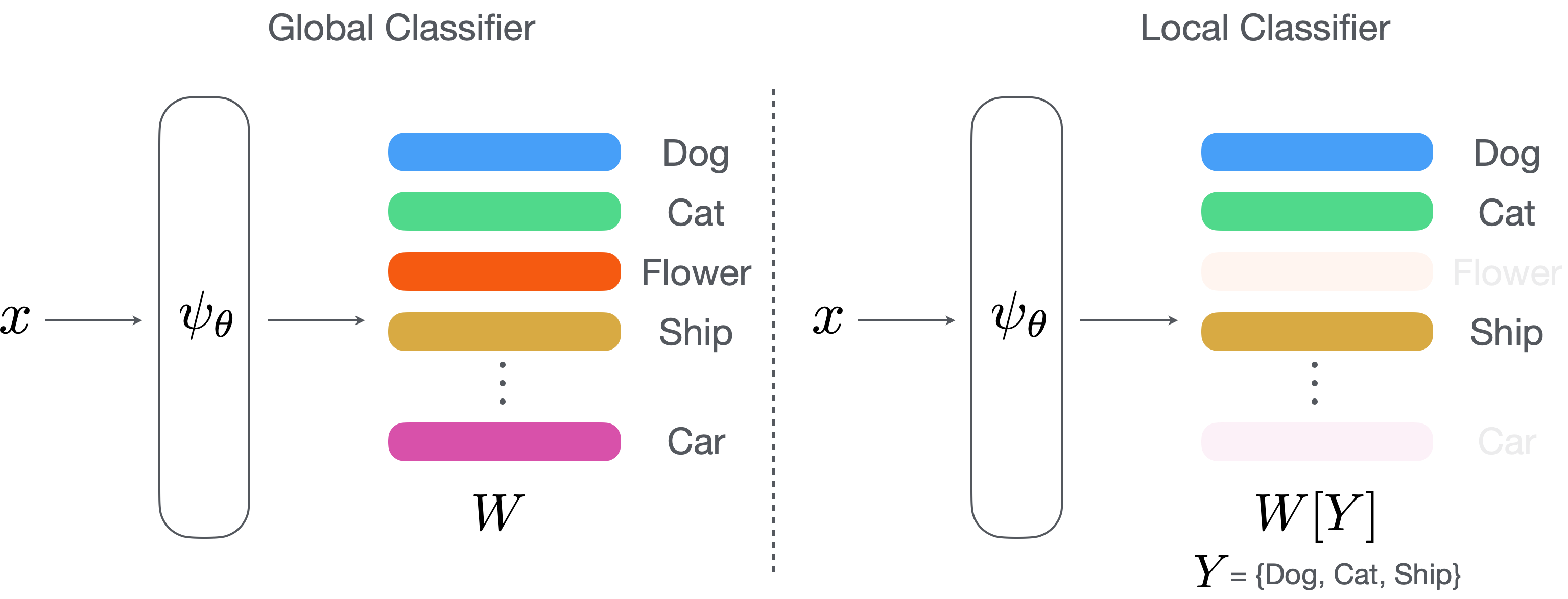
(b) Global to Local Classifier

Figure 1: (a) Colored squares represent samples. Tasks A and B can be “merged” meaningfully using global labels, but not local ones. (b) A global classifier can be used as local classifiers given the indices $Y$ of the intended classes to predict.

The standard FSL setting [e.g. 17, 48, 6] assumes access to a collection of tasks (i.e. the meta-training set) for training data. To perform pre-training, meta-training tasks must be merged into a flat dataset (see Sec. 2.3 for a formal definition), which implicitly assumes access to some notion of global labels shared across all tasks. However, global labels may be unavailable, such as when each task is independently labeled with only local labels. This renders naive task merging and pre-training infeasible (see Fig. 1a). Independent task annotation is a more realistic and general assumption, capturing scenarios when training tasks are collected organically from different sources rather than generated synthetically from a base dataset. Practical scenarios where naive task merging is infeasible include non-descriptive task labels (e.g. numerical ones) or concept overlap (e.g. marine animals vs mammals) among labels.

To tackle independent task annotation, we propose Meta Label Learning (MeLa), a novel algorithm that automatically infers a notion of latent global labels consistent with local task constraints. The inferred labels enable us to exploit pre-training for FSL, and to bridge the gap between experimental settings with or without access to global labels. Empirically, we demonstrate that MeLa is competitive with pre-training on oracle labels.

For experiments, we introduce a new Generalized FSL (GFSL) setting. In addition to independent task annotation, we also adopt a fixed-size meta-training set and enforce no repetition of samples across tasks. This challenging setting evaluates how efficiently meta-learning algorithms generalize from limited number of tasks, and prevents the algorithms from trivially uncover task relations by implicitly matching identical samples across tasks. We empirically show that MeLa performs robustly in both standard and GFSL settings, and clearly outperforms state-of-the-art models in the latter.

We summarize the main contributions below:

• We prove that pre-training relates to meta-learning as a loss upper bound. Consequently, minimizing the pre-training loss is a viable proxy for tackling meta-learning problems. Additionally, we identify meta-learning regimes where pre-training offers a clear improvement with respect to sample complexity. This theoretical analysis provides a principled explanation for pre-training’s empirical advantage.

• We propose MeLa, a general algorithm for inferring latent global labels from meta-training tasks. It allows us to exploit pre-training when global labels are absent or ill-defined.

• We propose an augmented pre-training procedure for FSL and a GFSL experimental setting.

• Extensive experiments demonstrate the robustness of MeLa. Detailed ablations provide deeper understanding of the model.

Extension of [78]

This paper is an extended version of [78] with the following contributions in addition to those of the original work: $i)$ a deeper theoretical insight into the role of pre-training from the perspective of the risk (rather than the empirical risk as in [78]), and quantifying its benefit in terms of sample complexity, $ii)$ the augmented training procedure for FSL, $iii)$ the GFSL experimental setting, $iv)$ significantly more empirical evidence to support the proposed algorithm.

2 Background

We formalize FSL as a meta-learning problem and review related methods. We also discuss the pre-training procedure adopted by many FSL methods.

2.1 Few-shot Learning using Meta-learning

FSL [16] considers a meta-training set of tasks $\mathcal{T}=\{(S_{t},Q_{t})\}_{t=1}^{T}$, with support set $S_{t}=\{(x_{j},y_{j})\}_{j=1}^{n_{s}}$ and query set $Q_{t}=\{(x_{j},y_{j})\}_{j=1}^{n_{q}}$ sampled from the same distribution. Typically, $S_{t}$ and $Q_{t}$ contain a small number of samples $n_{s}$ and $n_{q}$ respectively. We denote by ${\mathcal{D}}$ the space of datasets of the form $S_{t}$ or $Q_{t}$.

The meta-learning formulation for FSL aims to find the best base learner $\textrm{Alg}(\theta,\cdot):{\mathcal{D}}\to\mathcal{F}$ that takes as input support sets $S$, and outputs predictors $f=\textrm{Alg}(\theta,S)$, such that predictions $y=f(x)$ generalize well on the corresponding query sets $Q$. The base learner is meta-parameterized by $\theta\in\Theta$. Formally, the meta-learning objective for FSL is

$$\mathbb{E}_{(S,Q)\in\mathcal{T}}~{}\mathcal{L}\big{(}\textrm{Alg}(\theta,S),~{}Q\big{)},$$ (1)

where $\mathbb{E}_{(S,Q)\in\mathcal{T}}\triangleq\frac{1}{|\mathcal{T}|}\sum_{(S,Q)\in\mathcal{T}}$ is the empirical average over the meta-training set $\mathcal{T}$. The task loss $\mathcal{L}:{\mathcal{F}}\times{\mathcal{D}}\to{\mathbb{R}}$ is the empirical risk of the learner $f$ over query sets, based on some inner loss $\ell:{\mathcal{Y}}\times{\mathcal{Y}}\to{\mathbb{R}}$, where ${\mathcal{Y}}$ is the space of labels,

$$\mathcal{L}(f,D)~{}=~{}\mathbb{E}_{(x,y)\in D}~{}[\ell(f(x),y)].$$ (2)

Eq. 1 is sufficiently general to describe most existing methods. For instance, model-agnostic meta-learning (MAML) [17] parameterizes a model $f_{\theta}:{\mathcal{X}}\to{\mathcal{Y}}$ as a neural network, and $\textrm{Alg}(\theta,D)$ performs one (or more) steps of gradient descent minimizing the empirical risk of $f_{\theta}$ on $D$. Formally, given a step-size $\eta>0$,

$$f_{\theta^{\prime}}=\textrm{Alg}(\theta,D)\quad~{}\textrm{with}~{}\quad\theta^{\prime}=\theta-\eta~{}\nabla_{\theta}\mathcal{L}(f_{\theta},D).$$ (3)

Clearly, base learners $\textrm{Alg}(\theta,\cdot)$ is key to model performance and various strategies have been explored. Our proposed method is most closely related to meta-representation learning [55, 36, 6, 18], which parameterizes the base learner as $A(\theta,D)=w(g_{\theta}(D))g_{\theta}(\cdot)$, consisting of a global feature extractor $g_{\theta}:{\mathcal{X}}\to{\mathbb{R}}^{m}$ and a task-adaptive classifier $w:{\mathcal{D}}\to\{f:{\mathbb{R}}^{m}\to{\mathcal{Y}}\}$ that optimizes the following

$$\min_{\theta\in\Theta}~{}~{}\mathbb{E}_{(S,Q)\in\mathcal{T}}\left[\mathcal{L}\big{(}w(g_{\theta}(S)),g_{\theta}(Q)\big{)}\right]$$ (4)

where $g_{\theta}(D)\triangleq\{(g_{\theta}(x),y)~{}|~{}(x,y)\in D\}$ is the embedded dataset. Eq. 4 specializes 1 by learning a feature extractor $g_{\theta}$ shared (and fixed) among tasks. Only the classifier returned by $w(\cdot)$ adapts to the current task, in contrast to having the entire model $f_{\theta}:{\mathcal{X}}\to{\mathcal{Y}}$ adapted (e.g. 3 for MAML). While this may appear to restrict model adaptability, [55] has demonstrated that meta-representation learning matches MAML’s performance. Moreover, they showed that feature reuse is the dominant contributor to the generalization performance rather than adapting the representation to the task at hand.

The task-adaptive classifier $w(\cdot)$ may take various forms, including nearest neighbor [68], ridge regression classifier [6], embedding adaptation with transformer models [84], and Wasserstein distance metric [85]. In particular, the ridge regression estimator

$$w_{\rm ridge}(D){=}\operatornamewithlimits{argmin}_{W}~{}\mathbb{E}_{(x,y)\in D}~{}\left\|{Wx-y}\right\|^{2}{+}\lambda_{1}\left\|{W}\right\|_{F}^{2},$$ (5)

where $\left\|{\cdot}\right\|_{F}$ is the Frobenius norm, admits a differentiable closed-form solution and is computationally efficient for optimizing 4.

2.2 Conditional Meta-Learning

Conditional formulations of meta-learning [11, 77] extends Eq. 1 by considering base learners of the form $\textrm{Alg}(\tau(Z),S)$, where the meta-parameters $\theta=\tau(Z)$ is conditioned on some “contextual” information $Z\in\mathcal{Z}$ about the task $S$. Assuming each task in the meta-training set $\mathcal{T}$ to be equipped with such contextual information, 1 can be re-expressed as

$$\min_{\tau:\mathcal{Z}\to\Theta}~{}~{}\mathbb{E}_{(S,Q,Z)\in\mathcal{T}}~{}\mathcal{L}\big{(}\textrm{Alg}(\tau(Z),S),~{}Q\big{)},$$ (6)

namely the problem of learning a function $\tau:\mathcal{Z}\to\Theta$, which maps contextual information $Z\in\mathcal{Z}$ (e.g. a textual meta-description of the task/dataset) to a good task-specific base learner with parameters $\theta=\tau(Z)$.

The conditional formulation seeks to capture complex (e.g. multi-modal) distributions of meta-training tasks, and uses a unique base learner tailored to each one. In particular, [76, 83, 62] directly learn data-driven mappings from target tasks to meta-parameters, and [31] conditionally transforms feature representations based on a metric space trained to capture inter-class dependencies. Alternatively, [30] considers a mixture of hierarchical Bayesian models over the parameters of meta-learning models in order to condition on target tasks. In [77], Wang et al. showed that conditional meta-learning can be interpreted as a structured prediction problem and proposed a method leveraging structured prediction. From a more theoretical perspective, Denevi et al. [11, 12] proved that conditional meta-learning is theoretically advantageous compared to unconditional approaches by incurring smaller excess risk and being less prone to negative transfer. As we will discuss in Sec. 3, conditional meta-learning is closely related to our theoretical analysis on feature pre-training.

2.3 Feature Pre-training

Feature pre-training has been widely adopted in the recent meta-learning literature [e.g. 45, 50, 8, 77, 80, 82, 84, 4, 58, 69, 85, 1], and is arguably one of the key contributors to performance of state-of-the-art models. Instead of directly learning the feature extractor $g_{\theta}$ by optimizing 4, pre-training first learns a feature extractor via standard supervised learning.

Formally, the meta-training set $\mathcal{T}$ is “flattened” into $D_{\rm global}$ by merging all tasks:

$$D_{\rm global}=D(\mathcal{T})=\{(x_{i},y_{i})\}_{i=1}^{N}=\bigcup\limits_{(S,Q)\in\mathcal{T}}(S\cup Q),$$ (7)

where we have re-indexed the $(x_{i},y_{i})$ samples from $i=1$ to $N$ (the cumulative number of points from all support and query sets) to keep the notation uncluttered. Pre-training then learns the embedding function $g_{\theta}$ on $D_{\rm global}$ using the standard cross-entropy loss $\ell_{\rm ce}$ for multi-class classification:

$$(W_{N}^{\rm pre},\theta_{N}^{\rm pre})=\operatornamewithlimits{argmin}_{\theta,W}~{}\mathcal{L}(Wg_{\theta},D_{\rm global}).$$ (8)

where $W$ is the linear classifier over all classes. After pre-training, the feature extractor is either fixed [e.g. 62, 84, 77, 85, 71] or further adapted [e.g 4, 5, 21, 58] via meta-learning.

There is limited theoretical understanding and consensus on the effect of pre-training in FSL. In [62, 4, 82], the pre-training is only considered a standard pre-processing step for encoding the raw input and model performance is predominantly attributed to the proposed meta-learning algorithms. In [21] the authors similarly argued that meta-trained features are better than pre-trained ones, observing that adapting the pre-trained features with several base learners resulted in worse performance compared to the meta-learned features. In contrast, however, several works also empirically demonstrated that pre-training contributes significantly towards performance. [71] showed that combining the pre-trained features with suitable base learners already outperforms various meta-learning methods, while [15] observed that pre-training dominates top entries in 2021 Meta-learning Challenge.

We conclude by noting that recently pre-training has also been successfully applied to large-scale multi-modal settings combining visual and language input, enabling zero-shot learning [54], more flexible few-shot learning [2] (i.e., tasks may be described using free text), and generating more samples to augment FSL [81]. While this line of work further showcases the efficacy of pre-training strategies for FSL, in this work we focus on few shot learning settings with a single input modality.

3 Pre-training as Meta-learning

In this section, we characterize how feature pre-training relates to meta-learning as a loss upper bound. More precisely, we show that pre-training induces a special base learner with its corresponding meta-learning loss upper bounded by the cross-entropy loss $\ell_{\rm ce}$. Consequently, pre-training already produces a meta-representation suitable for FSL, matching the empirical results from [71, 84]. In addition, we show that pre-training incurs a smaller risk compared to its meta-learning counterpart, and more generally induces a conditional formulation that exploits contextual information for more robust learning.

3.1 Notation and Problem Setting

We consider a few-shot classification setting with a total of $C$ classes (global labels). Denote by $\mu$ the meta-distribution sampling distributions (a.k.a. tasks) $\rho$, from which we sample support and query sets $(S,Q)$ for each task. Each task distribution $\rho$ is associated with $k\leq C$ class labels $y_{\rho}^{(1)},\dots,y_{\rho}^{(k)}\in\{1,\dots,C\}$. Denote by $\rho_{Y}=\{y_{\rho}^{(1)},\dots,y_{\rho}^{(k)}\}$ the corresponding subset of $\{1,\dots,C\}$. Given a matrix $W\in{\mathbb{R}}^{C\times m}$ and a vector $Y\in\{1,\dots,C\}^{k}$ of indices, we denote by $W[Y]=W[\rho_{Y}]\in{\mathbb{R}}^{k\times m}$ the submatrix of $W$ obtained by selecting the rows corresponding to the unique indices $\rho_{Y}$ in $Y$. Lastly, Given a dataset $D=(x_{i},y_{i})_{i=1}^{n}$ we denote by $D_{Y}\in\{1,\dots,C\}^{n}$ the vector with entries corresponding to the labels $y_{i}$.

We also define the expected error incurred by a meta-learning algorithm solving 4

$${\mathcal{E}}(\theta,\mu)=\mathbb{E}_{\rho\sim\mu}~{}\mathbb{E}_{(S,Q)\sim\rho}~{}\mathcal{L}(w(g_{\theta}(S)),g_{\theta}(Q)).$$ (9)

This is the meta-learning risk incurred by a meta-parameter $\theta$, namely the error incurred by training the classifier via $w(g_{\theta}(S))$ (e.g. Eq. 5) and testing it on the query set $g_{\theta}(Q)$, averaged over $(S,Q)$ pairs sampled from tasks $\rho$, which in turn are sampled from meta-distribution $\mu$. The risk is the ideal error we wish to minimize.

3.2 Global Label Selection (GLS)

We start our analysis by introducing a special FSL scenario that will be useful for understanding the relation between pre-training and meta-learning. To this end, we assume in this scenario that global labels are available to the model.

Given the access to global labels, we can design a new algorithm that learns a single global multi-class linear classifier $W$ at the meta-level (i.e. shared across all tasks), and simply selects the required rows $W[S_{Y}]$ when tackling a task. More formally, we can define a special base learner called global label selector (GLS) such that

$$\textrm{Alg}((W,\theta),S)=\textrm{GLS}(W,\theta,S)=W[S_{Y}]g_{\theta}(\cdot).$$

Illustrated in Fig. 1b, this “algorithm” does not solve an optimization problem on the support set $S$, but only selects the subset of rows of $W$ corresponding to the classes present in $S$ as the task-specific classifier.

Since $W$ and $\theta$ are now both shared across all tasks, we may learn them jointly by minimizing the following

$$\mathbb{E}_{(S,Q)\in\mathcal{T}}~{}\mathcal{L}(W[S_{Y}]g_{\theta}(\cdot),Q),$$ (10)

over both $W$ and $\theta$. This strategy, to which we refer as meta-GLS, learns both the representation and linear classifier at the meta-level, with the sole task-specific adaptation process being the selection of columns of $W$ using the global labels.

GLS Finds a Good Meta-representation

Learning a global $W$ shared among multiple tasks (rather than having each classifier $w(g_{\theta}(S))$ accessing exclusively the tasks’ training data), can be very advantageous for generalization. This is evident when the (global) classes are separable for a meta-representation $g_{\theta}$. Let

$${\mathcal{E}}_{\textrm{\tiny GLS}}(W,\theta,\mu)=\mathbb{E}_{\rho\sim\mu}~{}\mathbb{E}_{(S,Q)\sim\rho}~{}\mathcal{L}(W[S_{Y}]g_{\theta}(\cdot),Q),$$ (11)

denote the expected meta-GLS risk incurred by the minimizer of 10. Then, for any inner algorithm $w(\cdot)$, we have

$$\min_{W}~{}{\mathcal{E}}_{\textrm{\tiny GLS}}(W,\theta,\mu)\leq{\mathcal{E}}(\theta,\mu),$$ (12)

namely that, for any given representation $g_{\theta}$, finding a global classifier $W$ for all classes is more favorable than solving each task in isolation. In other words, solving meta-GLS provides a good representation $g_{\theta}(\cdot)$ for standard meta-learning problem.

3.3 Pre-training and GLS

Existing works such as [71, 15] demonstrates that pre-training offers a robust alternative to learn the meta-representation $g_{\theta}(\cdot)$. We will show that GLS is related to pre-training, under some mild assumptions.

Assumption 1.

The meta-distribution $\mu$ samples tasks $\rho$. Sampling from each $\rho$ is performed as follows:

1. For each $j\,{\in}\,\{1,\dots,k\}$ and class $y_{\rho}^{(j)}\,{\in}\,\rho_{Y}$, we sample $n$ examples $x_{1}^{(j)},\dots,x_{n}^{(j)}$ i.i.d. from a conditional distribution $\pi(x|y\,{=}\,y_{\rho}^{(j)})$ shared across all tasks. All generated pairs are collected in the support set $S=(x_{i}^{(j)},y_{\rho}^{(j)})_{i,j=1}^{n,k}$.

2. The query set $Q$ is generated by sampling $m$ points i.i.d. from $\pi_{\rho}(x,y)$, namely $Q\sim\pi_{\rho}^{m}$ with

   $$\pi_{\rho}(x,y)=\pi(x|y)\mathrm{Unif}_{\rho}(y)$$ (13)

   and $\mathrm{Unif}_{\rho}$ the uniform distribution over the labels in $\rho_{Y}$.

In essence, Assumption 1 characterizes the standard process of constructing meta-training tasks for FSL, typically adopted to build pre-training datasets in practice. In particular, let $\pi_{\mu}(x,y)$ be the marginal probability of observing $(x,y)$ in the meta-training tasks, i.e. firstly sampling a task $\rho$ from $\mu$, followed by sampling a class $y$ uniformly by $\mathrm{Unif}_{\rho}(\cdot)$ and finally $x$ by $\pi(\cdot|y)$. It then follows that sampling a dataset $D_{\rm global}$ from $\pi_{\mu}$ is equivalent to sample a meta-training set $\mathcal{T}$ from $\mu$ and flatten it into $D(\mathcal{T})$ according to the pre-training procedure described in 7.

We can therefore introduce the (global) multi-class classification risk associated to $\pi_{\mu}$

$$\mathcal{L}(Wg_{\theta}(\cdot),\pi_{\mu})=\mathbb{E}_{(x,y)\sim\pi_{\mu}}~{}\ell_{\rm ce}(Wg_{\theta}(x),y).$$ (14)

The above risk can be seen as the ideal objective for the pre-training estimator in 8. In addition, the following result relates pre-training to meta-GLS.

Theorem 1.

Under Assumption 1, let $\pi_{\mu}(x,y)$ be the marginal distribution of observing $(x,y)$ in the meta-training set. Then, for any (global) classifier $W$,

$${\mathcal{E}}_{\textrm{\tiny GLS}}(W,\theta,\mu)\leq\mathcal{L}(W,\theta,\pi_{\mu}).$$ (15)

Moreover, if the global classes are separable,

$$\min_{W,\theta}~{}{\mathcal{E}}_{\textrm{\tiny GLS}}(W,\theta,\mu)=\min_{W,\theta}~{}\mathcal{L}(W,\theta,\pi_{\mu}).$$ (16)

The result shows that the GLS error is upper bounded by the global multi-class classification error. Hence, minimizing the global multi-class classification error also indirectly minimizes the meta-learning risk. This implies that pre-training implicitly learns a meta-representation suitable for FSL.

3.4 Generalization Properties

Thm. 1 shows that under the class-separability assumption, pre-training is equivalent to performing meta-GLS. We now study which of the two approaches is more sample-efficient from a generalization perspective.

Let $(W_{T}^{\textrm{\tiny GLS}},\theta_{T}^{\textrm{\tiny GLS}})$ denote the meta-parameters learned by an algorithm minimizing 10 over a dataset $\mathcal{T}$ comprising of $T$ separate tasks. Applying standard results from statistical learning theory, we can obtain excess risk bounds characterizing the quality of $\theta_{T}$’s predictions in terms of the number $T$ of tasks the algorithm has observed in training. For instance, following [65, Chapter 26] we have that in expectation with respect to sampling $\mathcal{T}$

$$\mathbb{E}_{\mathcal{T}}[{\mathcal{E}}_{\textrm{\tiny GLS}}(W_{T}^{\textrm{\tiny GLS}},\theta_{T}^{\textrm{\tiny GLS}},\mu)] \leq\min_{(W,\theta)\in\Omega}~{}{\mathcal{E}}_{\textrm{\tiny GLS}}(W,\theta,\mu)+2L_{\textrm{\tiny GLS}}\mathfrak{R}_{T}(\Omega)$$

$$\leq\min_{(W,\theta)\in\Omega}~{}{\mathcal{E}}_{\textrm{\tiny GLS}}(W,\theta,\mu)+\frac{2L_{\textrm{\tiny GLS}}C_{\Omega}}{\sqrt{T}}$$

where $L_{\textrm{\tiny GLS}}$ denotes the Lipschitz constant of ${\mathcal{E}}_{\textrm{\tiny GLS}}$, while $\Omega\subset{\mathbb{R}}^{m\times C}\times\Theta$ is the space of hypotheses for the multi-class classifier $Wg_{\theta}(\cdot)$. Here, $\mathfrak{R}_{T}(\Omega)$ is the Rademacher complexity of $\Omega$ [65], which measures the overall potential expressivity of an estimator that can be trained over them. For neural networks, [22] showed that $\mathfrak{R}_{T}(\Omega)$ may be further bounded by $\mathfrak{R}_{T}(\Omega)\leq C_{\Omega}/\sqrt{T}$, where $C_{\Omega}$ is a constant depending on the specific neural architecture, with deeper networks having a larger constant. The bound indicates that the risk incurred by GLS becomes closer to that of the ideal meta-parameters as the number of observed tasks $T$ grows.

We can apply the same Rademacher-based bounds to 14 and the pre-training estimator from 8, obtaining that in expectation with respect to sampling $\mathcal{T}$

$$\mathbb{E}_{\mathcal{T}}[\mathcal{L}(W_{N}^{\rm pre},\theta_{N}^{\rm pre},\pi_{\mu})]\leq\min_{(W,\theta)\in\Omega}~{}\mathcal{L}(W,\theta,\pi_{\mu})+\frac{2L_{\textrm{\rm pre}}C_{\Omega}}{\sqrt{N}}$$

where $N$ is the number of samples in $D_{\rm global}$ and $L_{\textrm{\rm pre}}$ is the Lipschitz constant of the global multi-class classification risk. By combining the above bound with the result from Thm. 1 we conclude that

$$\mathbb{E}_{\mathcal{T}}[~{}{\mathcal{E}}_{\textrm{\tiny GLS}}(W_{N}^{\rm pre},\theta_{N}^{\rm pre},\mu)]\leq\min_{W,\theta}~{}{\mathcal{E}}_{\textrm{\tiny GLS}}(W,\theta,\mu)+\frac{2L_{\textrm{\rm pre}}C_{\Omega}}{\sqrt{N}},$$

which is an excess risk bound analogous to that obtained for meta-GLS. The key difference is that the bound above depends on the number $N$ of total samples in $D_{\textrm{global}}$, rather that the total number $T$ of tasks.

Comparing the rates of meta-GLS and the pre-training estimator, we observe that typically $N\gg T$ (for instance $N=nT$ when each task has the same number of $n$ samples). Additionally, since $L_{\mathrm{pre}}$ is comparable or smaller than $L_{\textrm{\tiny GLS}}$ (see Appendix B), we conclude that

Given exactly the same data ($\mathcal{T}$ for meta-GLS and $D(\mathcal{T})$ for pre-training), pre-training achieves a much smaller error than meta-GLS.

For instance, in the case of a 5-way-5-shot FSL problem, pre-training improves upon the meta-GLS bound on excess risk by a factor of $\sqrt{N/T}=\sqrt{n}=\sqrt{100}=10$.

Given the relation between GLS and standard meta-learning that we highlighted in Sec. 3.2, our analysis provides a strong theoretical argument in favor of adopting pre-training in meta-learning settings. To our knowledge, this is a novel and surprising result.

3.5 Connection to Conditional Meta-Learning

More generally, we observe that GLS is also an instance of conditional meta-learning: the global labels of the task provide additional contextual information about the task to facilitate model learning. Global labels directly reveal how tasks relate to one another and in particular if any classes to be learned are shared across tasks. GLS thus simply map global labels of tasks to task classifiers via $W[S_{Y}]$. In contrast, unconditional approaches (e.g. R2D2 [6], ProtoNet [48]) learn classifiers by minimizing some loss over support sets, losing out on the access to the contextual information provided by global labels.

In addition to our result, [11, 12] also proved that conditional meta-learning is advantageous over the unconditional formulation by incurring a smaller excess risk, especially when the meta-distribution of tasks is organized into distant clusters. We refer readers to the original papers for a detailed discussion. In practice, global labels provide clustering of task samples for free and improve regularization by enforcing each cluster (denoted by global label $y_{\rho}^{j}$) to share classifier parameters $W[y_{\rho}^{j}]$ across all tasks. This provides further explanation to why pre-training yields a robust meta-representation with strong generalization performance.

3.6 Leveraging Pre-training in Practice

The goal of meta-learning is to generalize to novel classes unseen during training. Therefore, practical FSL applications assume meta-testing and meta-training distributions to share no class labels. To apply our analysis in Sec. 3.4 to these settings, we may follow the theoretical approach in [13] and assume that meta-training and meta-testing classes share a common representation. The assumption is reasonable since extensive empirical evidences demonstrate that pre-trained representation on meta-training set is robust for directly classifying novel classes [71, 15]. To prevent overfitting on meta-training set and ensure a robust represntation for meta-testing, well-established techniques [e.g., 3, 77, 71] include imposing $\ell_{2}$ regularization during pre-training (see weight decay in Appendix C.2) and early stopping by performing meta validation.

While pre-training might offer a powerful initial representation $\theta$ – as highlighted by our analysis in Sec. 3.4 – it may be advisable to further improve $\theta$. One general strategy is to fine-tune $\theta$ by directly optimizing 4 using the desired classifier to tackle novel classes [e.g. 84, 60, 85, 72]. This strategy is known as meta fine-tuning. A different approach is based on a transfer learning perspective. Specifically, [33, 66, 38] showed that careful task-specific fine-tuning (e.g., limiting the number of learnable parameters) from a pre-trained representation achieves robust generalization performance, even in FSL settings. We investigate both strategies in our experiments.

4 Methods

In this section, we propose three practical algorithms motivated by our theoretical analysis. In Sec. 4.1, we introduce an augmentation procedure for pre-training to further improve representation learning in image-based tasks. In Sec. 4.2, we tackle the scenario where global labels are absent by automatically inferring a notion of global labels. Lastly, we introduce a meta fine-tuning procedure in Sec. 4.3 to investigate how much meta-learning could improve the pre-trained representation.

4.1 Augmented Pre-training for Image-based Tasks

In general, pre-training is a standard process with well-studied techniques for improving the final learned representation. Many of these techniques, including data augmentation [8], auxiliary losses [45] and model distillation [71], are also effective for FSL (i.e. the learned representation is suitable for novel classes during meta-testing). In particular, we may interpret data augmentation techniques as increasing $N$ in the bounds for the pre-training estimator outlined in Sec. 3.4, thus improving the error incurred by pre-training and consequently the learned representation $g_{\theta}$.

In addition to standard augmentations (e.g. random cropping and color jittering) investigated in [8], we further propose an augmented procedure for pre-training via image rotation. For every class $y_{i}$ in the original dataset, we create three additional classes by rotating all images of class $y_{i}$ by $r\in\{90^{\circ},180^{\circ},270^{\circ}\}$ respectively. All rotations are multiples of $90^{\circ}$ such that they can be implemented by basic operations efficiently (e.g. flip and transpose) and prevent pre-training from learning any trivial features from visual artifacts produced by arbitrary rotations [20]. Pre-training is then performed normally on the augmented dataset.

The augmented dataset quadruples the number of samples and classes compared to the original dataset. According to our analysis from Sec. 3.4, pre-training on the augmented dataset may yield a more robust representation. Further, we also hypothesize that the quality of the representation also depends on the number of classes available in the pre-training dataset, since classifying more classes requires learning increasingly discriminating representations. Our experiments show that 1) augmented pre-training consistently outperforms the standard one, and 2) quality of the learned representation depends on both the dataset size and the number of classes available for training.

4.2 Meta Label Learning

The ability to exploit pre-training crucially depends on access to global labels. However, as discussed in Sec. 1, global labels may be inaccessible in practical applications. For instance when meta-training tasks are collected and annotated independently. Additionally, tasks may have conflicting labels over similar data points based on different task requirements – a setting illustrated by our experiments in Sec. 5.4. Therefore in some applications, global labels are ill-defined, and pre-training is not directly applicable.

To tackle this problem, we consider the more general setting where only local labels from each task are known. This setting is also the one originally adopted by most earlier works in meta-learning [e,g 17, 68, 75, 39, 6, 36]. In the local label setting, we propose Meta Label Learning (MeLa), which automatically infer a notion of latent global labels across tasks. The inferred labels enable pre-training and thus bridge the gap between the experiment settings with and without global labels. We stress that our proposed method does not replace standard pre-training with global labels, but rather provides a way to still benefit from such a strategy when they are absent.

Algorithm 1 MeLa

  Input: meta-training set $\mathcal{T}=\{S_{t},Q_{t}\}_{t=1}^{T}$

  $g_{\theta}^{\rm sim}=\operatornamewithlimits{argmin}_{g_{\theta}}\mathbb{E}_{(S,Q)\in\mathcal{T}}\left[\mathcal{L}(w(g_{\theta}(S)),g_{\theta}(Q)\right])$

  Global clusters $G=\textrm{LearnLabeler}(\mathcal{T},g_{\theta}^{\textrm{sim}})$

  $g_{\theta}^{\rm pre}=\textrm{Pretrain}(D(\mathcal{T}),G)$

  $g_{\theta}^{*}=\textrm{MetaFinetune}(G,\mathcal{T},g_{\theta}^{\rm pre})$

  Return $g_{\theta}^{*}$

Alg. 1 outlines the general approach for learning a few-shot model using MeLa: we first meta-learn an initial representation $g_{\theta}^{\rm sim}$; Secondly, we cluster all task samples using $g_{\theta}^{\rm sim}$ as a feature map while enforcing local task constraints. The learned clusters are returned as inferred global labels. Using the inferred labels, we can apply pre-training to obtain $g_{\theta}^{\rm pre}$, which may be further fine-tuned to derive the final few-shot model $g_{\theta}^{*}$. We present in Sec. 4.3 a simple yet effective meta fine-tuning procedure.

For learning $g_{\theta}^{\rm sim}$, we directly optimize 4 using ridge regression 5 as the base learner. We use ridge regression for its computational efficiency and good performance. Using $g_{\theta}^{\rm sim}$ as a base for a similarity measure, the labeling algorithm takes as input the meta-training set and outputs a set of clusters as global labels. The algorithm consists of a clustering routine for sample assignment and centroid updates and a pruning routine for merging small clusters.

Clustering

The clustering routine leverages local labels for assigning task samples to appropriate global clusters and enforcing task constraints. We observe that for any task, the local labels describe two constraints: 1) samples sharing a local label must be assigned to the same global cluster, while 2) samples with different local labels must not share the same global cluster. To meet constraint 1, we assign all samples $\{x^{(j)}_{i}\}_{i=1}^{n}$ of class $y_{\rho}^{(j)}$ to a single global cluster by

$$v^{*}=\operatornamewithlimits{argmin}_{v\in\{1,\dots,V\}}\left\|{\frac{1}{n}\sum_{i=1}^{n}g_{\theta}^{\rm sim}(x_{i}^{(j)})-g_{v}}\right\|^{2},$$ (17)

with $V$ being the current number of centroids.

We apply 17 to all classes $y_{\rho}^{(1)},\dots,y_{\rho}^{(k)}$ within a task. If multiple local classes map to the same global label, we simply discard the task to meet constraint 2. Otherwise, we proceed to update the centroid $g_{v^{*}}$ and sample count $N_{v^{*}}$ for the matched clusters using

$$\begin{split}g_{v^{*}}&\leftarrow\frac{N_{v^{*}}g_{v^{*}}+\sum_{i=1}^{n}g_{\theta}^{\rm sim}(x_{i})}{N_{v^{*}}+n},\\ N_{v^{*}}&\leftarrow N_{v^{*}}+n,\end{split}$$ (18)

Pruning

We also introduce a strategy for pruning small clusters. We model the sample count of each cluster as a binomial distribution $N_{v}\propto B(T,p)$. We set $p=\frac{1}{V}$, assuming that each cluster is equally likely to be matched by a local class of samples. Any cluster with a sample count below the following threshold is discarded,

$$N_{v}<\bar{N_{v}}-q\sqrt{\textrm{Var}(N_{v})}$$ (19)

where $\bar{N_{v}}$ is the expectation of $N_{v}$, $\textrm{Var}(N_{v})$ the variance, and $q$ a hyper-parameter controlling how aggressive the pruning is.

Algorithm 2 LearnLabeler

  Input: embedding model $g_{\theta}^{\mathrm{sim}}$, meta-training set $\mathcal{T}=\{S_{t},Q_{t}\}_{t=1}^{T}$, number of classes in a task $k$

  Initialization: sample tasks from $\mathcal{T}$ to initialize clusters $G=\{g_{v}\}_{v=1}^{V}$,

  While $|G|$ has not converged:

   $N_{v}=1$ for each $g_{v}\in G$

   For $(S,Q)\in\mathcal{T}$:

    Match $S\cup Q$ to its centroids $M\,{=}\,\{g_{q}\}_{q=1}^{K}$ using 17

    If $M$ has $k$ unique clusters

     Update centroid $g_{q}$ for each $g_{q}\in M$ via 18

   $G\leftarrow\{g_{v}|g_{v}\in G,N_{v}\geq\textrm{threshold in }$19$\}$

  Return $G$

Alg. 2 outlines the full labeling algorithm. We first initialize a large number of clusters by setting their centroids with mean class embeddings from random classes in $\mathcal{T}$. For $V$ initial clusters, $\lceil\frac{V}{k}\rceil$ tasks are needed since each task contains $k$ classes and could initialize as many clusters. The algorithm then alternates between clustering and pruning to refine the clusters and estimate the number of clusters jointly. The algorithm terminates and returns the current clusters $G$ when the number of clusters does not change from the previous iteration. Using clusters $G$, local classes from the meta-training set can be assigned global labels with nearest neighbor matching using 17. For tasks that fail to map to $k$ unique global labels, we simply exclude them from the pre-training process.

The key difference between Alg. 2 and the classical $K$-means algorithm [42] is that the proposed clustering algorithm exploits local information to guide the clustering process, while $K$-means algorithm is fully unsupervised. We will show in the experiments that enforcing local constraints is necessary for learning robust meta-representation.

Alg. 2 also indirectly highlights how global labels, if available, offer valuable information about meta-training set. In addition to revealing precisely how input samples relate to one another across tasks, global labels provide an overview of meta-training set, including the desired number of clusters and their sizes. In contrast, Alg. 2 needs to estimate both properties when only local labels are given.

Time Complexity

The time complexity of training MeLa is dominated by the computational cost of pretraining, accounting for over $70\%$ of the overall running time. From our benchmarks, the time complexity of MeLa is comparable to those of the current state-of-the-art methods based on pre-training [e.g., 84, 80] and significantly more efficient than methods relying on complex base learners [e.g., 85]. We refer to Sec. C.3 for a more detailed discussion and comparison with [84, 80, 85].

When global labels are not available MeLa requires performing an additional inference step to estimate them. While this stage accounts for around 20% of the total running time, we observe in Sec. 5 that it provides a significant performance boost compared to FSL methods not utilizing pre-training, which are the only applicable ones in the absence of global labels.

4.3 Meta Fine-Tuning

As discussed in Sec. 3.6, while pre-training already yields a robust meta-representation for FSL, it is desirable to adapt the pre-trained representation such that the new meta-representation better matches the base learner intended for novel classes. We call this additional training meta fine-tuning, which is adopted by several state-of-the-art FSL models [85, 84, 77, 37].

For meta fine-tuning, existing works suggest that model performance depends crucially on preserving the pre-trained representation. In particular, [62, 77, 37] all keep the pre-trained representation fixed, and only learn a relatively simple transformation on top for the new base learners. Additionally, [21] showed that meta fine-tuning the entire representation model lead to worse performance compared to standard meta-learning, negating the advantages of pre-training completely.

We thus present a simple residual architecture that preserves the pre-trained embeddings and allows adaptation for the new base learner. Formally, we consider the following parameterization for a fine-tuned meta-learned embedding $g_{\theta}^{*}$,

$$g_{\theta}^{*}(x)=g_{\theta}^{\rm pre}(x)+h(g_{\theta}^{\rm pre}(x))$$ (20)

where $g_{\theta}^{\rm pre}$ is the pre-trained representation and $h$ a learnable function (e.g. a small fully connected network). We again use 5 as the base learner and optimizes 4 directly. Our experiments show that the proposed fine-tuning process achieves results competitive with more sophisticated base learners, indicating that the pre-trained representation is the predominant contributor to good test performance.

5 Experiments

We evaluate MeLa on various benchmark datasets and compare it with existing methods. The experiments are designed to address the following questions:

• How does MeLa compare to existing methods for generalization performance? We also introduce the more challenging GFSL setting in Sec. 5.2.

• How do different model components (e.g. pre-training, meta fine-tuning) contribute to generalization performance?

• Does MeLa learn meaningful clusters? Can MeLa handle conflicting task labels?

• How can we improve the quality of the pre-trained representation?

• How robust is MeLa to hyper-parameter choices?

5.1 Benchmark Datasets

Mini/tiered-ImageNet. [75, 57] has become default benchmark for FSL. Both datasets are subsets of ImageNet [61] with miniImageNet having 60K images over 100 classes, and tieredImageNet having 779K images over 608 classes. Following previous works, we report performance on 1- and 5-shot settings, using 5-way classification tasks.

Variants of mini/tiered-ImageNet

We introduce several variants of mini/tiered-ImageNet to better understand MeLa and more broadly the impacts of dataset configuration on pre-training. Specifically, we create mini-60 that consists of 640 classes and 60 samples per class. Mini-60 contains the same number of samples as miniImageNet, though with more classes and fewer samples per class. Mini-60 keeps the same meta-test set as miniImageNet to ensure a fair comparison of test performance of model trained on each dataset in turn. We designed mini-60 to investigate the behavior of MeLa when encountering a dataset with a high number of base classes and low number of samples per base class. We also use mini-60 to explore how data diversity present in the training data affects the learned representation. Analogous to mini-60, we also introduce tiered-780 as a variant to tieredImageNet, where we take the total number of samples in tieredImageNet and calculate the number of samples over the full 1000 ImageNet classes, excluding those used in the meta-test set of tieredImageNet.

Meta-Dataset

[72] is a meta-learning classification benchmark combining 10 widely used datasets: ILSVRC-2012 (ImageNet) [61], Omniglot [35], Aircraft [44], CUB200 [79], Describable Textures (DTD) [10], QuickDraw [32], Fungi [64], VGG Flower (Flower) [49], Traffic Signs [28] and MSCOCO [40]. We use Meta-Dataset to construct several challenging experiment scenarios, including learning a unified model for multiple domains and learning from tasks with conflicting labels.

5.2 Experiment Settings

The standard FSL setting [17, 68, 84, 80, 5] assumes that a meta-distribution of tasks is available for training. This translates to meta-learners having access to an exponential number of tasks synthetically generated from the underlying dataset, a scenario unrealistic for practical applications. Recent works additionally assume access to global labels in order to leverage pre-training, in contrast with earlier methods that assume access to only local labels. We will highlight such differences when comparing different methods.

Generalized Few-Shot Learning (GFSL) Setting

We introduce a more challenging and realistic FSL setting. Specifically, we only allow access to local labels, since global ones may be inaccessible or ill-defined. In addition, we employ a no-replacement sampling scheme when synthetically generating tasks from the underlying dataset. This sampling process limits the meta-training set to a fixed-size, a standard assumption for most machine learning problems. The fixed size also enables us to evaluates the sample efficiency of different methods. Secondly, no-replacement sampling prevents MeLa and other meta-learners from trivially learning task relations, a key objective of meta-learning, by matching same samples across tasks. For instance, an identical sample appearing in multiple tasks would allow MeLa to trivially cluster local classes. Lastly, the sampling process reflects any class imbalance in the underlying dataset, which might present a more challenging problem.

5.3 Performance Comparison in Standard Setting

We compare MeLa to a diverse group of existing methods on mini- and tieredImageNet in Tab. I. We separate the methods into those requiring global labels and those that do not. We note that the two groups of methods are not directly comparable since global labels provides a significant advantage to meta-learners as discussed previously. The method groupings are intended to demonstrate the effect of pre-training on generalization performance.

TABLE I: Test accuracy of meta-learning models on miniImageNet and tieredImageNet.

	miniImageNet		tieredImageNet
	$1$-shot	$5$-shot	$1$-shot	$5$-shot
Global Labels
Simple CNAPS [5]	$53.2\pm-$	$70.8\pm-$	$63.0\pm-$	$80.0\pm-$
LEO [62]	$61.7\pm 0.7$	$77.6\pm 0.4$	$66.3\pm 0.7$	$81.4\pm 0.6$
TASML [77]	$62.0\pm 0.5$	$78.2\pm 0.5$	$66.4\pm 0.4$	$82.6\pm 0.3$
RFS [71]	$62.0\pm 0.4$	$79.6\pm 0.3$	$69.4\pm 0.5$	$84.4\pm 0.3$
ProtoNet (with pre-train) [80]	$62.4\pm 0.2$	$80.5\pm 0.1$	$68.2\pm 0.2$	$84.0\pm 0.3$
Meta-Baseline [9]	$63.2\pm 0.2$	$79.3\pm 0.2$	$68.6\pm 0.3$	$83.7\pm 0.2$
FEAT [84]	$\mathbf{66.7\pm 0.2}$	$82.0\pm 0.1$	$70.8\pm 0.2$	$84.8\pm 0.2$
FRN [80]	$66.4\pm 0.2$	$\mathbf{82.8\pm 0.1}$	$\mathbf{71.2\pm 0.2}$	$\mathbf{86.0\pm 0.2}$
DeepEMD [85]	$65.9\pm 0.8$	$82.4\pm 0.6$	$\mathbf{71.2\pm 0.9}$	$\mathbf{86.0\pm 0.6}$
Local Labels
MAML [17]	$48.7\pm 1.8$	$63.1\pm 0.9$	$51.7\pm 1.8$	$70.3\pm 0.8$
ProtoNet [68]	$49.4\pm 0.8$	$68.2\pm 0.7$	$53.3\pm 0.9$	$72.7\pm 0.7$
R2D2 [6]	$51.9\pm 0.2$	$68.7\pm 0.2$	$65.5\pm 0.6$	$80.2\pm 0.4$
MetaOptNet [36]	$62.6\pm 0.6$	$78.6\pm 0.5$	$66.0\pm 0.7$	$81.5\pm 0.6$
Shot-free [56]	$59.0\pm{\rm n/a}$	$77.6\pm{\rm n/a}$	$63.5\pm{\rm n/a}$	$82.6\pm{\rm n/a}$
MeLa (pre-train only)	$64.5\pm 0.4$	$81.5\pm 0.3$	$69.5\pm 0.5$	$84.3\pm 0.3$
MeLa	$\mathbf{65.8\pm 0.4}$	$\mathbf{82.8\pm 0.3}$	$\mathbf{70.5\pm 0.5}$	$\mathbf{85.9\pm 0.3}$

Tab. I clearly shows that “global-labels” methods leveraging pre-training generally outperform “local-labels” methods except MeLa. We highlight that the re-implementation of ProtoNet in [80] benefits greatly from pre-training, outperforming the original by over 10% across the two datasets. Similarly, while RFS and R2D2 both learn a fixed representation and only adapt the classifier based on each task, RFS’s pre-trained representation clearly outperforms R2D2’s meta-learned representation. We further note that state-of-the-art methods such as DeepEMD and FEAT are heavily reliant on pre-training and performs drastically worse in GFSL setting, as we will discuss in Sec. 5.4.

In the local-labels category, MeLa outperforms existing methods thanks to its ability to still exploit pre-training using the inferred labels. MeLa achieves about 4% improvement over the next best method in all settings. Across both categories, MeLa obtains performance competitive to state-of-the-art methods such as FRN, FEAT and DeepEMD despite having no access to global labels. This indicates that MeLa is able to infer meaningful clusters to substitute global labels and obtains performance similar to methods having access to global labels. We will provide further quantitative results on the clustering algorithm in Sec. 5.7. Lastly, we note that MeLa also outperforms several methods from the “global-label” category, such as RFS and Meta-Baseline. We attribute MeLa’s better performance to more robust representation via augmented pre-training and our formulation for meta fine-tuning. In particular, we explicitly preserve the pre-trained representation using residual connections, in contrast to meta fine-tuning the entire representation model as in ProtoNet and Meta-Baseline. Consistent with [21], the results suggest that meta fine-tuning the entire representation model could negate the advantages of pre-training shown in our theoretical analysis.

5.4 Performance Comparison in Generalized Setting

We evaluate a representative set of few-shot learners under GFSL. For this setting, we introduce two new experimental scenario using Meta-Dataset to simulate task heterogeneity.

In the first scenario, we construct the meta-training set from Aircraft, CUB and Flower, which we simply denote as ”Mixed”. Tasks are sampled independently from one of the three datasets. For meta-testing, we sample 1500 tasks from each dataset and report the average accuracy. The chosen datasets are intended for fine-grained classification in aircraft models, bird species and flower species respectively. Thus the meta-training tasks share the broad objective of fine-grained classification, but are sampled from three distinct domains. A key challenge of this scenario is to learn a unified model across multiple domains, without any explicit knowledge about them or the global labels.

TABLE II: Test Accuracy on Aircraft, CUB and VGG Flower (Mixed dataset). A single model is trained for each method over all tasks.

	Aircraft		CUB		VGG Flower		Average
	1-shot	5-shot	1-shot	5-shot	1-shot	5-shot	1-shot	5-shot
ProtoNet [68]	$35.1\pm 0.4$	$51.0\pm 0.5$	$32.7\pm 0.4$	$46.4\pm 0.5$	$56.7\pm 0.5$	$73.8\pm 0.4$	$41.7\pm 0.7$	$57.5\pm 0.7$
MatchNet [75]	$31.4\pm 0.4$	$39.4\pm 0.5$	$42.7\pm 0.5$	$54.1\pm 0.5$	$62.5\pm 0.5$	$70.0\pm 0.1$	$45.7\pm 0.1$	$54.5\pm 0.1$
R2D2 [6]	$67.7\pm 0.6$	$82.8\pm 0.4$	$53.8\pm 0.5$	$69.2\pm 0.5$	$65.4\pm 0.5$	$83.3\pm 0.3$	$61.9\pm 0.5$	$78.6\pm 0.4$
DeepEMD [85]	$34.7\pm 0.7$	$47.8\pm 1.4$	$39.3\pm 0.7$	$52.1\pm 1.4$	$61.3\pm 0.9$	$74.5\pm 1.4$	$45.1\pm 0.7$	$58.1\pm 1.2$
FEAT [84]	$61.7\pm 0.6$	$75.8\pm 0.5$	$59.6\pm 0.6$	$73.1\pm 0.5$	$62.9\pm 0.6$	$76.0\pm 0.4$	$60.9\pm 0.7$	$75.0\pm 0.5$
FRN [80]	$60.7\pm 0.7$	$77.6\pm 0.5$	$61.9\pm 0.7$	$77.7\pm 0.5$	$65.2\pm 0.6$	$81.2\pm 0.5$	$63.1\pm 0.7$	$79.7\pm 0.5$
MeLa	$\mathbf{78.2\pm 0.5}$	$\mathbf{89.5\pm 0.3}$	$\mathbf{73.8\pm 0.6}$	$\mathbf{88.7\pm 0.3}$	$\mathbf{76.6\pm 0.4}$	$\mathbf{91.5\pm 0.2}$	$\mathbf{76.2\pm 0.3}$	$\mathbf{89.9\pm 0.2}$

Tab. II show that MeLa outperforms all baselines under GFSL setting. In particular, MeLa achieves a large margin of 10% improvement over the baselines, including state-of-the-art models FEAT, FRN and DeepEMD, which performed competitively against MeLa in Tab. I. In particular, FEAT and DeepEMD performed noticeably worse, indicating the methods’ reliance on pre-trained representation and the difficulty of meta-learning from scratch with complex base learners. FRN outperforms FEAT and DeepEMD, as it is designed to also work without pre-training.

In the second scenario, we consider meta-training tasks with heterogeneous objectives, leading to conflicting task-labels and consequently ill-defined global labels. For the Aircraft dataset, each sample from the base dataset has three labels associated with it, including variant, model and manufacturer that form a hierarchy. We sample tasks based on each of the three labels and creates a meta-training set containing three different task objectives: classifying fine-grained differences between model variants, classifying different airplanes, and classifying different airplane manufacturers. To differentiate from the original dataset, we refer to this meta-training set as H-Aircraft. The training data is particularly challenging given the competing goals across different tasks: a learner is required to recognize fine-grained differences between airplane variants, while being able to identify general similarities within the same manufacturer. The meta-training data also reflects the class imbalance of underlying dataset, with samples from Boeing and Airbus over-represented.

TABLE III: Test accuracy on H-Aircraft in the generalized setting.

	$1$-shot	$5$-shot
ProtoNet [68]	$47.8\pm 0.5$	$66.8\pm 0.5$
MatchNet [75]	$65.6\pm 0.2$	$78.7\pm 0.2$
R2D2	$75.1\pm 0.3$	$86.4\pm 0.2$
DeepEMD [85]	$51.3\pm 0.5$	$65.6\pm 0.8$
FEAT [84]	$77.6\pm 0.6$	$87.3\pm 0.4$
FRN [80]	$81.9\pm 0.4$	$91.0\pm 0.2$
MeLa	$\mathbf{84.8\pm 0.3}$	$\mathbf{92.9\pm 0.2}$
Oracle	$84.4\pm 0.3$	$93.1\pm 0.2$

Tab. III shows that MeLa outperforms all baselines for H-Aircraft. To approximate the oracle performance when ground truth labels were given, we optimize a supervised semantic softmax loss [59] over the hierarchical labels. Specifically, we train the (approximate) oracle to minimize a multi-task objective combining individual cross entropy losses over the three labels. MeLa performs competitively against the oracle, indicating the robustness of the proposed labeling algorithm in handling ill-defined labels and class imbalance.

The experimental results suggest that MeLa performs robustly in both the standard and GFSL settings. In contrast, baseline methods perform noticeably worse in the latter, due to the absence of pre-training and limited training data.

Connection to theoretical results

We comment on the empirical results so far in relation to our theoretical analysis. The empirical results strongly indicate that pre-training produces robust meta-representations for FSL by exploiting contextual information from global labels. This is consistent with our observation that pre-training would achieve a smaller error than its meta-learning counterpart. On the other hand, the results also validate our hypothesis that the pre-trained representation can be further improved, since the pre-trained representation is not explicitly optimized for handling novel classes. In particular, FEAT, FRN, DeepEMD and MeLa all outperform the pre-trained representation from [71] by further adapting it.

5.5 Performance Comparison on Meta-Dataset

We further evaluate MeLa on the full Meta-Dataset to assess our method’s generalization performance. We adopt the experiment setting of training on ImageNet only and testing on all meta-test sets [72], to clearly evaluate out-of-distribution generalization. We note that state-of-the-art methods [e.g. 38, 73, 63] on Meta-Dataset are heavily reliant on pre-training with global labels, while MeLa only has access to a collection of FSL tasks and has to infer such labels. In Tab. IV, we compare MeLa with state-of-the-art methods including fine tuning [72], ALFA+fo-Proto-MAML [72], BOHB [63], FLUTE [73] and TSA [38].

The results show that MeLa is able to effectively infer meaningful global labels and achieve robust generalization to novel datasets, achieving an average accuracy of 68.5%. Despite not being given global labels for pre-training, MeLa only trails behind TSA while outperforming other methods. In addition, we note that the task-specific tuning adopted by TSA is orthogonal – but compatible – to MeLa: by combining MeLa with TSA (see Sec. C.2 for details) we are able to further improve our generalization performance, outperforming the original TSA approach on 10 out of the 13 meta-test sets (Tab. IV last column). These results further demonstrate the robustness of MeLa in learning robust representations over a large number of FSL tasks, and the efficacy of task-specific fine-tuning in improving generalization of novel tasks.

TABLE IV: Test accuracy on Meta-Dataset, training on ImageNet only, using ResNet-18 for all models.

Test Dataset Finetune [72] fo-Proto-MAML [72] BOHB [63] FLUTE [73] Meta-Baseline [9] TSA [38] MeLa MeLa+TSA ImageNet $45.8\pm 1.1$ $52.8\pm 1.1$ $51.9\pm 1.1$ $46.9\pm 1.1$ $59.2\pm-$ $57.4\pm 1.0$ $59.3\pm 1.1$ $\mathbf{61.3\pm}1.1$ Omniglot $60.9\pm 1.6$ $61.9\pm 1.5$ $67.6\pm 1.2$ $61.6\pm 1.4$ $69.1\pm-$ $74.2\pm 1.2$ $66.2\pm 1.4$ $\mathbf{74.8\pm}1.4$ Aircraft $68.7\pm 1.3$ $63.4\pm 1.1$ $54.1\pm 0.9$ $48.5\pm 1.0$ $54.1\pm-$ $66.1\pm 1.0$ $67.9\pm 1.0$ $\mathbf{80.7\pm}1.1$ Birds $57.3\pm 1.3$ $69.8\pm 1.1$ $70.7\pm 0.9$ $47.9\pm 1.0$ $77.3\pm-$ $73.9\pm 0.9$ $78.7\pm 0.8$ $\mathbf{81.6\pm}0.9$ Textures $69.0\pm 0.9$ $70.8\pm 0.9$ $68.3\pm 0.8$ $63.8\pm 0.8$ $76.0\pm-$ $76.2\pm 0.7$ $77.0\pm 0.8$ $\mathbf{78.9\pm}0.8$ QuickDraw $42.6\pm 1.2$ $59.2\pm 1.2$ $50.3\pm 1.0$ $57.5\pm 1.0$ $57.3\pm-$ $64.6\pm 0.9$ $64.3\pm 1.0$ $\mathbf{71.5\pm}1.0$ Fungi $38.2\pm 1.0$ $41.5\pm 1.2$ $41.4\pm 1.1$ $31.8\pm 1.0$ $45.4\pm-$ $46.8\pm 1.1$ $\mathbf{47.3\pm}1.2$ $47.3\pm 1.2$ VGG Flower $85.5\pm 0.7$ $86.0\pm 0.8$ $87.3\pm 0.6$ $80.1\pm 0.9$ $89.6\pm-$ $91.3\pm 0.5$ $89.9\pm 0.7$ $\mathbf{93.5\pm}0.8$ Traffic Sign $66.8\pm 1.3$ $60.8\pm 1.3$ $51.8\pm 1.0$ $46.5\pm 1.1$ $66.2\pm-$ $82.5\pm 0.9$ $65.4\pm 1.1$ $\mathbf{86.9\pm}1.0$ MSCOCO $34.9\pm 1.0$ $48.1\pm 1.1$ $48.0\pm 1.0$ $41.4\pm 1.0$ $\mathbf{55.7\pm}-$ $55.2\pm 1.0$ $54.2\pm 1.1$ $54.4\pm 1.1$ MNIST - - - $80.8\pm 0.8$ - $94.0\pm 0.5$ $88.1\pm 0.6$ $\mathbf{94.6\pm}0.6$ CIFAR-10 - - - $65.4\pm 0.8$ - $\mathbf{79.4\pm}0.8$ $70.4\pm 0.8$ $76.9\pm 0.8$ CIFAR-100 - - - $52.7\pm 1.1$ - $\mathbf{70.5\pm}0.9$ $62.0\pm 1.0$ $69.3\pm 0.9$ Average 57.0 61.4 59.1 55.8 65.0 71.7 68.5 74.7 Average Rank 6.0 5.2 5.6 6.5 4.0 2.4 3.0 1.3

5.6 Ablations on Pre-training

Given the significance of pre-training on final performance, we investigate how the rotation data augmentation and data configuration impact the performance of the pre-trained representation. We focus on the effects of dataset sizes and the number of classes present in the dataset.

Rotation-Augmented Pre-training

In Sec. 4.1, we proposed to increase both the size and the number of classes in a dataset via input rotation. By rotating the input images by the multiples of $90^{\circ}$, we quadruple both the size and the number of classes in a dataset. In Tab. V, we compare the performance of standard pre-training against the rotation-augmented one, for multiple datasets. We use the inferred labels from MeLa for pre-training.

TABLE V: Test accuracy comparison between pre-trained representations: standard vs. rotation-augmented

	$1$-shot		$5$-shot
	standard	rotation	standard	rotation
miniImageNet	$62.0\pm 0.4$	$64.5\pm 0.4$	$79.6\pm 0.3$	$81.5\pm 0.3$
mini-60	$63.9\pm 0.7$	$67.7\pm 0.5$	$81.5\pm 0.5$	$84.1\pm 0.5$
tieredImageNet	$69.1\pm 0.5$	$69.5\pm 0.6$	$83.9\pm 0.3$	$84.3\pm 0.4$
tiered-780	$78.0\pm 0.6$	$78.2\pm 0.6$	$89.9\pm 0.4$	$90.1\pm 0.4$
H-Aircraft	$79.2\pm 0.5$	$84.8\pm 0.3$	$89.4\pm 0.3$	$92.9\pm 0.2$

The results suggest that rotation-augmented pre-training consistently improves the quality of the learned representation. It achieves over 3% improvements in both miniImageNet and H-aircraft, while obtains about 0.5% in tieredImageNet. It is clear that rotation augmentation works the best with smaller datasets with fewer classes. As the dataset increases in size and diversity, the additional augmentation has less impact on the learned representation.

Effects of Class Count

We further evaluate the effects of increasing number of classes in a dataset while maintaining the dataset size fixed. For this, we compare the performance of miniImageNet and tieredImageNet with their respective variants mini-60 and tiered-780.

Tab. V suggests that given a fixed size dataset, having more classes improves the quality of the learned representation compared to having more samples per class. We hypothesize that classifying more classes lead to more discriminative and robust features, while standard $\ell_{2}$ regularization applied during pre-training prevents overfitting despite having fewer samples per class.

Overall, the experiments suggest that pre-training is a highly scalable process where increasing either data diversity or dataset size will lead to more robust representation for FSL. In particular, the number of classes in the dataset appears to play a more significant role than the dataset size.

5.7 Ablations on The Clustering Algorithm

The crucial component of MeLa is Alg. 2, which infers a notion of global labels and allows pre-training to be exploited in GFSL setting. We perform several ablation studies to better understand Alg. 2.

The Effects of No-replacement Sampling

We study the effects of no-replacement sampling, since it affects both the quality of the similarity measure through $g_{\theta}^{\rm sim}$ and the number of tasks available for inferring global clusters. The results are shown in Tab. VI.

TABLE VI: The effects of no-replacement sampling on the clustering algorithm

Dataset	miniImageNet		tieredImageNet		mini-60
Replacement	Yes	No	Yes	No	Yes	No
Tasks Clustered (%)	100	98.6	99.9	89.5	98.7	97.8
Clustering Acc (%)	100	99.5	96.4	96.4	72.8	70.1
1-shot Acc (%)	$65.8\pm 0.4$	$65.8\pm 0.5$	$70.5\pm 0.5$	$70.5\pm 0.5$	$68.4\pm 0.7$	$68.4\pm 0.5$
5-shot Acc (%)	$82.8\pm 0.3$	$82.8\pm 0.4$	$85.9\pm 0.3$	$85.9\pm 0.3$	$84.0\pm 0.5$	$84.0\pm 0.5$

In Tab. VI, clustering accuracy is computed by assigning the most frequent ground truth label in each cluster as the desired target. Percentage of tasks clustered refers to the tasks that map to $k$ unique clusters by Alg. 2. The clustered tasks satisfy both constraints imposed by local labels and are used for pre-training.

For both sampling processes, MeLa achieves comparable performances across all three datasets. This indicates the robustness of Alg. 2 in inferring suitable labels for pre-training, even when task samples do not repeat across tasks. This shows that Alg. 2 is not trivially matching identical samples across task, but relying on $g_{\theta}^{\rm sim}$ for estimating sample similarity. We note that mini-60 is particularly challenging under no-replacement sampling, with only 384 tasks in the meta-training set over 640 ground truth classes.

Effects of Pruning Threshold

In Alg. 2, the pruning threshold is controlled by the hyper-parameter $q$. We investigate how different $q$ values affect the number of clusters estimated by the algorithm and the corresponding test accuracy. Tab. VII suggest that MeLa is robust to a wide range of $q$ and obtains representations similar to that produced by the ground truth labels. While it is possible to replace $q$ with directly guessing the number of clusters in Alg. 2, we note that tuning for $q$ is more convenient since appropriate $q$ values appear to empirically concentrate within a much narrower range, compared to the possible numbers of global clusters present in a dataset.

TABLE VII: Test accuracy (pre-train only) and cluster count for various pruning thresholds, 5-shot setting

miniImageNet (64 classes)			tieredImageNet (351 classes)			mini-60 (640 classes)
Oracle Pre-train: 81.5%			Oracle Pre-train: 84.5%			Oracle Pre-train: 85.2%
$q$	No. Clusters	MeLa	$q$	No. Clusters	MeLa	$q$	No. Clusters	MeLa
3	64	$81.5\pm 0.4$	3.5	351	$84.3\pm 0.4$	4.5	463	$84.0\pm 0.4$
4	75	$81.1\pm 0.4$	4.5	373	$84.1\pm 0.3$	5.5	462	$83.8\pm 0.4$
5	93	$80.9\pm 0.4$	5.5	444	$84.0\pm 0.5$	6.5	472	$84.0\pm 0.4$

Inferred Labels vs. Oracle Labels

From Tabs. VI and VII, we observe that it may be unnecessary to fully recover the oracle labels (when they exists). For mini-60, MeLa inferred 463 clusters over 640 classes, which implies mixing of the oracle classes. However, the inferred labels still perform competitively against the oracle labels, suggesting the robustness of the proposed method. The results also suggest that we may improve the recovery of the oracle labels by sampling more tasks from the meta-distribution.

The Importance of Local Constraints

Alg. 2 enforces consistent assignment of task samples given their local labels. To understand the importance of enforcing these constraints, we consider an ablation study where Alg. 2 is replaced with the standard $K$-means algorithm. The latter is fully unsupervised and ignores any local constraints. We initialize the $K$-means algorithm with 64 clusters for miniImageNet and 351 clusters for tieredImageNet, matching the true class counts in respective datasets.

TABLE VIII: Test Accuracy (Pre-train only) using Alg. 2 vs. $K$-mean Clustering

	miniImageNet			tieredImageNet
Cluster Alg.	Cluster Acc	1-shot	5-shot	Cluster Acc	1-shot	5-shot
Alg. 2 (MeLa)	100	$64.5\pm 0.4$	$81.5\pm 0.3$	96.4	$69.5\pm 0.5$	$84.3\pm 0.3$
$K$-mean	84.9	$60.7\pm 0.5$	$76.9\pm 0.3$	28.2	$64.8\pm 0.6$	$78.8\pm 0.5$

Tab. VIII indicates that enforcing local constraints is critical for generalization performance during meta-testing. In particular, test accuracy drops by over 5% for tieredImageNet, when the $K$-means algorithm ignores local task constraints. Among the two constraints, we note that 17 appears to be the more important one since nearly all tasks automatically match $K$ unique clusters in our experiments (see tasks clustered in Tab. VI).

Domain Inference for multi-domain tasks

In addition to inferring global labels, We may further augment Alg. 2 to infer the different domains present in a meta-training set, if we assume that all samples within a task belongs to a single domain. Given the assumption, two global clusters are connected if they both contain samples from the same task. This is illustrated in Fig. 2a. Consequently, inferred clusters form an undirected graph with multiple connected components, with each representing a domain. We apply the above algorithm to the multi-domain Mixed Dataset consisting of Aircraft, CUB and Flower.

Fig. 2b visualizes the inferred domains on the multi-domain scenario. For each inferred cluster, we project its centroid onto a 2-dimensional point using UMAP [46]. Each connected component is assigned a different color. Despite some mis-clustering within each domain, we note that Alg. 2 clearly separates the three domains present in the meta-training set and recovers them perfectly.

Domain inference is important for multi-domain scenario as it enables domain-specific pre-training. Recent works [e.g. 41, 37, 14] on Meta-Dataset have shown that combining domain-specific representation into a universal representation is empirically more advantageous than training on all domains together. Lastly, we remark that multi-domain meta-learning is also crucial for obtaining robust representation suitable for wider range of novel tasks, including cross-domain transfer.

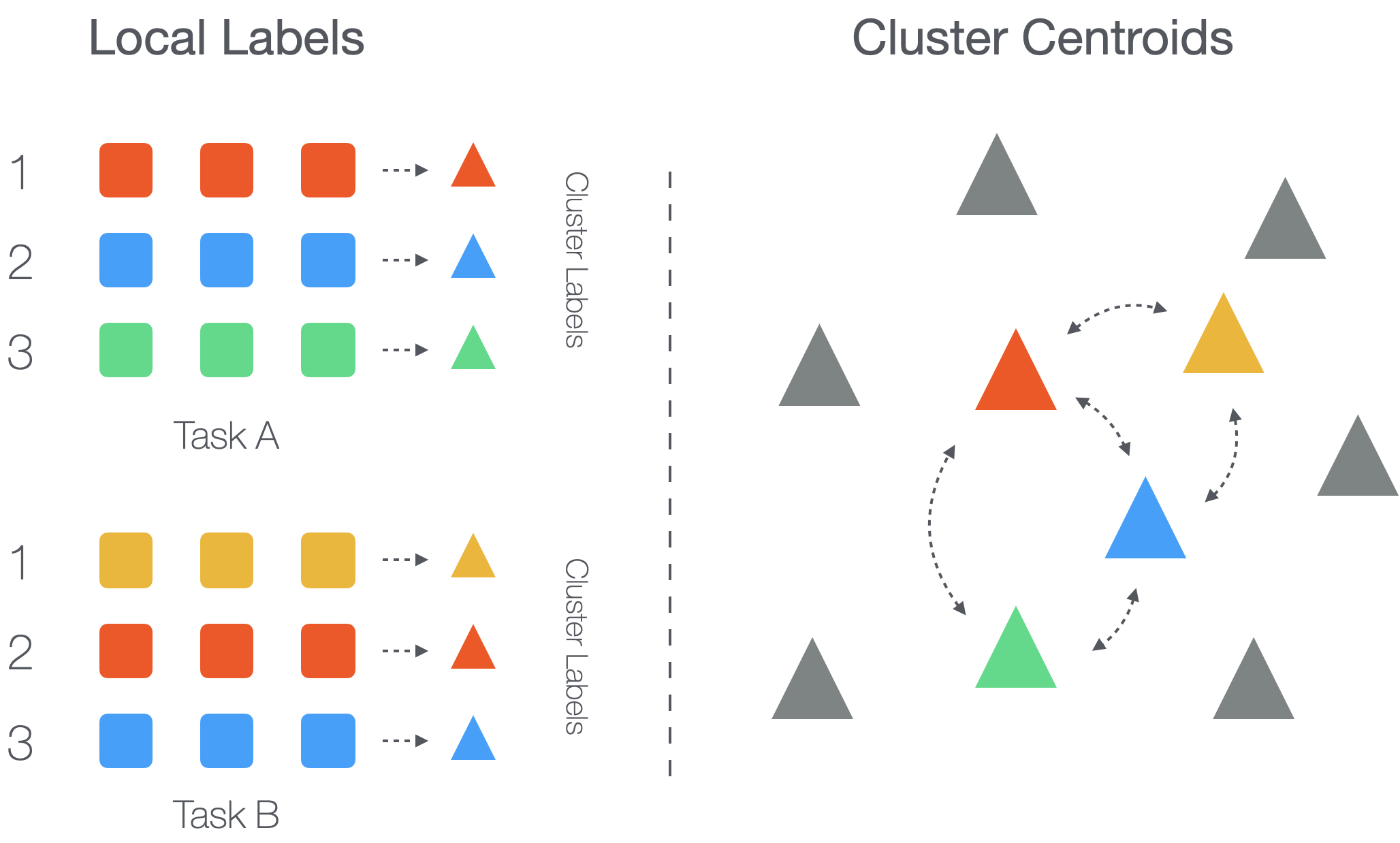
(a) Domain Inference via Connected Components

(b) UMAP visualization of different domains in multi-domain dataset

Figure 2: (a) The coloured clusters (red, green, blue and yellow) are connected since they both contains samples from the same task. Domains can be inferred by computing the connected components of the inferred clusters. (b) UMAP visualization of the three inferred domains from the 5-shot Mixed dataset containing Aircraft, CUB and VGG. Circles are the means (using the pretrained features) of the instances in each task averaged per local class while triangles are the learned centroids, all vectors are embedded using UMAP. The three domains are recovered perfectly.

6 Conclusion

In this work we focused on the role played by pre-training in meta-learning applications, with particular attention to few-shot learning problems. Our analysis was motivated by the recent popularity of pre-training as a key stage in most state-of-the-art FSL pipelines. We first investigated the benefits of pre-training from a theoretical perspective. We showed that in some settings this strategy enjoys significantly better sample complexity than pure meta-learning approaches, hence offering a justification for its empirical performance and wide adoption in practice.

We then proceeded to observe that pre-training requires access to global labels of the classes underlying the FSL problem. This might not always be possible, due to phenomena like heterogeneous labeling (i.e. multiple labelers having different labeling strategies) or contextual restrictions like privacy constraints. We proposed Meta-Label Learning (MeLa) as a strategy to address this concern. We compared MeLa with state-of-the-art methods on a number of tasks including well-established standard benchmarks as well as new datasets we designed to capture the above limitations on task labels. We observed that MeLa is always comparable or better than previous approaches and very robust to lack of global labels or the presence of conflicting labels.

More broadly, our work provides a solid foundation for understanding existing FSL methods, in particular the vital contribution of pre-training towards generalization performance. We also demonstrated that pre-training scales well with the size of datasets and data diversity, which in turn leads to more robust few-shot models. Future research may focus on further theoretical understanding of pre-training and better pre-training processes.

Ruohan Wang is a research scientist at Institute for Infocomm Research, A*STAR Singapore. Previously, he was a postdoctoral researcher at UCL’s Intelligent Systems Group, supervised by Prof. Massimiliano Pontil. He completed his Ph.D. in machine learning at Imperial College under the supervision of Prof. Yiannis Demiris and Prof. Carlo Ciliberto, funded by Singapore National Science Scholarship. He has a broad interests in topics of machine learning, including representation learning, meta-learning, and imitation learning. His research goal is to design robust ML systems that could efficiently leverage past experiences and existing knowledge for future learning.

John Isak Texas Falk is a Ph.D student at the Dept. of Computer Science of UCL where he is supervised by Prof. Massimiliano Pontil and Prof. Carlo Ciliberto. He is also a Research Fellow at Italian Institute of Technology CSML under the supervision of Prof. Massimiliano Pontil. His Ph.D is focused on few-shot and meta-learning in the context of kernel learning and statistical learning theory in the context of meta-learning, although he has an interest in representation learning, fairness and bandits. The goal of his research is how to design robust meta-learning systems that work well under real-world conditions and come with guarantees.

Massimiliano Pontil is Senior Researcher at the Italian Institute of Technology (IIT), where he leads the Computational Statistics and Machine Learning group, and co-director of the ELLIS Unit Genoa, a joint effort of IIT and the University of Genoa. He is also part-time professor at University College London and member of the UCL Centre for Artificial Intelligence. He obtained his PhD in Physics from the University of Genoa in 1999. He has made significant contributions to machine learning, particularly in the areas of kernel methods, multitask and transfer learning, sparsity regularization and statistical learning theory. He has published about 150 papers at international journals and conferences, is regularly on the programme committee of the main machine learning conferences, and has been on the editorial board of the Machine Learning Journal, Statistics and Computing, and JMLR. He has held visiting positions at a number of universities and research institutes, including the Massachusetts Institute of Technology, the Isaac Newton Institute for Mathematical Sciences in Cambridge, the City University of Hong Kong, the University Carlos III de Madrid, ENSAE Institute Polytechnique Paris, and Ecole Polytechnique.

Carlo Ciliberto is Associate Professor with the Centre for Artificial Intelligence at University College London, He is member of the ELLIS society and of the ELLIS Unit based at UCL. He obtained his bachelor and master degrees in Mathematics at the Università Roma Tre (Magna Cum Laude) and a PhD in machine learning applied to robotics and computer vision at the Istituto Italiano di Tecnologia. He has been Postdoctoral Researcher at the Massachusetts Institute of Technology with the Center for Brain Minds and Machines and became Lecturer (Assistant Professor) at Imperial College London before joining UCL, where he now carries out his main research activity. Carlo’s research interests focus on foundational aspects of machine learning within the framework of statistical learning theory. He is particularly interested in the role of “structure” (being it in the form of prior knowledge or structural constraints) in reducing the sample complexity of learning algorithms with the goal of making them more sustainable both computationally and financially. He investigated these questions within the settings of structured prediction, multi-task and meta-learning, with applications to computer vision, robotics and recommendation systems.

Appendix A Proof for Theorem 1

We first restate the notations and assumptions necessary to prove Thm. 1. From Assumption 1, we define the joint distribution $\pi_{\mu}(x,y)$ as the probability of observing an input-output pair $(x,y)$ when first sampling a task $\rho$ from $\mu$ and then sampling $(x,y)$ according to the “query” distribution $\pi_{\rho}$ in 13. In other words, $\pi_{\mu}(x,y)=\pi(x|y)\textrm{Unif}_{\rho}(y)\mu(\rho)$ is the marginal distribution of $(x,y)$ with respect to $\rho$.

We observe that for any $g:{\mathcal{X}}\times{\mathcal{Y}}\to{\mathbb{R}}$,

$$\mathbb{E}_{(x,y)\sim\pi_{\mu}}~{}g(x,y)=\mathbb{E}_{\rho\sim\mu}\mathbb{E}_{(x,y)\sim\pi_{\rho}}~{}g(x,y).$$ (21)

Given Assumption 1, $S$ and $Q$ are sampled independently by the task $\rho$. In particular the marginal $\rho_{Q}$ of $\rho$ with respect to $Q$ corresponds to $\pi_{\rho}$. Similarly, we denote $\rho_{S}$ the distribution over support sets obtained by marginalizing out the query set. We report one remark following the assumption above.

Remark 1.

For any task $\rho$ and any algorithm $D\mapsto f_{D}$ returning functions $f_{S}:{\mathcal{X}}\to{\mathbb{R}}^{k}$, we have

$$\mathbb{E}_{(S,Q)\sim\rho}~{}\mathcal{L}(f_{S},Q) =\mathbb{E}_{S\sim\rho_{S}}\mathbb{E}_{Q\sim\pi_{\rho}^{m}}~{}\mathcal{L}(f_{S},Q)$$

$$=\mathbb{E}_{S\sim\rho_{S}}\mathbb{E}_{Q\sim\pi_{\rho}^{m}}\frac{1}{m}\sum_{(x,y)\in Q}\ell(f_{S}(x),y)$$

$$=\mathbb{E}_{S\sim\rho_{S}}\mathbb{E}_{(x,y)\sim\pi_{\rho}}~{}\ell(f_{S}(x),y)$$

$$=\mathbb{E}_{S\sim\rho_{S}}~{}\mathcal{L}(f_{S},\pi_{\rho}),$$

where for any $f:{\mathcal{X}}\to{\mathbb{R}}^{k}$ we have denoted by

$$\mathcal{L}(f,\pi_{\rho})=\mathbb{E}_{(x,y)\sim\pi_{\rho}}~{}\ell(f_{S}(x),y),$$

the expected risk of a function $f:{\mathcal{X}}\to{\mathbb{R}}^{k}$ with respect to the loss $\ell$ and the distribution $\pi_{\rho}$.

Using the above remark, we shows how the GLS risk for the meta-distribution $\mu$ is related to multi-class classification risk for the corresponding multi-class distribution $\pi_{\mu}$. See 1

Proof.

We start by studying the GLS risk for a pair $(W,\theta)$ of meta-parameters. By expanding the GLS objective explicitly with Remark 1, we have

$${\mathcal{E}}_{\textrm{\tiny GLS}}(W,\theta,\mu) =\mathbb{E}_{\rho\sim\mu}~{}\mathcal{L}_{\rm ce}(\textrm{\tiny GLS}(W,\theta,\rho),\pi_{\rho})$$

$$=\mathbb{E}_{\rho\sim\mu}~{}\mathbb{E}_{(x,y)\sim\pi_{\rho}}~{}\ell_{\rm ce}(\textrm{\tiny GLS}(W,\theta,\rho)(x),y)$$

$$=\mathbb{E}_{\rho\sim\mu}~{}\mathbb{E}_{(x,y)\sim\pi_{\rho}}~{}\ell_{\rm ce}(W[\rho_{Y}]\psi_{\theta}(x),y).$$

Since $\rho_{Y}$ is a subset of $\{1,\dots,C\}$, by definition of cross-entropy we have

$$\ell_{\rm ce}(W[\rho_{Y}]\psi_{\theta}(x),y) =-\log\frac{\exp(W[y]\psi_{\theta}(x))}{\sum_{y^{\prime}\in\rho_{Y}}\exp(W[y^{\prime}]\psi_{\theta}(x))}$$

$$\leq-\log\frac{\exp(W[y]\psi_{\theta}(x))}{\sum_{y^{\prime}\in\{1,\dots,C\}}\exp(W[y^{\prime}]\psi_{\theta}(x))}$$

$$=\ell_{\rm ce}(W\psi_{\theta}(x),y).$$

We can now apply 21 where we take $g(x,y)=\ell_{\rm ce}(W\psi_{\theta}(x),y)$. Then,

$$\mathbb{E}_{\rho\sim\mu}~{}\mathbb{E}_{(x,y)\sim\pi_{\rho}}~{}\ell_{\rm ce}(W\psi_{\theta}(x),y)=\mathbb{E}_{(x,y)\sim\pi_{\mu}}~{}\ell_{\rm ce}(W\psi_{\theta}(x),y)=\mathcal{L}_{\rm ce}(W,\theta,\pi_{\mu}),$$

which concludes the proof for 15.

Now, if the global classes are linearly separable, we have

$$\min_{W,\theta}~{}\mathcal{L}(Wg_{\theta},\pi_{\mu})=0.$$ (22)

Since $\ell_{ce}(\cdot)$ is non-negative, combining 22 and 15 yields

$$0\leq\min_{W,\theta}~{}{\mathcal{E}}_{\rm GLS}(W,\theta)\leq\min_{W,\theta}~{}\mathcal{L}(Wg_{\theta},\pi_{\mu})=0$$ (23)

from which (16) follows. ∎

Appendix B Comparison between the Lipschitz Constants of ${\mathcal{E}}_{\textrm{\tiny GLS}}$ and $\mathcal{L}$

In this section, we compare the Lipschitz constants associated to the meta-GLS risk and the pre-training objective function discussed in Sec. 3.4, showing that $L_{\rm pre}$ is comparable or smaller than $L_{\textrm{\tiny GLS}}$.

We recall that the Lipschitz constant of an objective function of the form $\mathbb{E}_{\xi\sim\rho}\ell(\cdot,\xi)$ is $\sup_{\xi}L_{\xi}$, where $L_{\xi}$ is the Lipschitz constant of $\ell(\cdot,\xi)$ for any $\xi$ in the support of the probability $\rho$, denoted as $\textrm{supp}\rho$. Furthermore, we recall that if $\ell(\cdot,\xi)$ is smooth on its domain $\Omega$ then the Lipschitz constant of $\mathbb{E}_{\xi\sim\rho}\ell(\cdot,\xi)$ can be characterized as

$$\sup_{\begin{subarray}{c}\omega\in\Omega\\ \xi\in\textrm{supp}\rho\end{subarray}}\left\|{\nabla_{\omega}\ell(\omega,\xi)}\right\|,$$

In the following we will assume $\Omega=B_{\lambda}^{2,1}(0)\times\Theta$, where $B_{\lambda}(0)$ is a ball of radius $\lambda$ with respect to the $2,1$–norm centred at $0$, namely that $\left\|{W}\right\|_{2,1}\leq\lambda$. The $2,1$–norm is defined as $\left\|{W}\right\|_{2,1}=\sum_{z\leq C}\left\|{W_{z}}\right\|_{2}$ and helps to simplify the following analysis. $\Theta$ is the space of parameters for $g_{\theta}$ and we assume the representation model to be normalized, namely $\left\|{g_{\theta}(x)}\right\|=1$ for all $\theta\in\Theta$ and $x\in{\mathcal{X}}$. The normalized representational model could be easily generalized to any bounded representation, namely $\sup_{\theta,x}\left\|{g_{\theta}(x)}\right\|<+\infty$.

We now compare the Lipschitz constants of ${\mathcal{E}}_{\textrm{\tiny GLS}}$ in 11 and the pre-training risk 14. The key difference between the two objective functions is that meta-GLS applies the cross-entropy loss over subsets of $\{1,\dots,C\}$ classes at each time (the classes appearing in a given task), while global multi-class classification applies it to the entire set of $C$ classes. Therefore, to highlight the dependency on the number of classes in the following we denote $\ell_{\rm ce}^{k}$ the cross entropy evaluated among $k$ classes for $k$ an integer. Then, under the notation introduced in this section and in Sec. 3.4, we need to compare

$$L_{\textrm{\tiny GLS}}=\sup_{\begin{subarray}{c}(W,\theta)\in\Omega\\ (S,Q)\in\textrm{supp}\tilde{\mu}\end{subarray}}~{}\left\|{\nabla_{W,\theta}~{}\mathcal{L}(W[S_{Y}]g_{\theta}(\cdot),Q)}\right\|=\sup_{\begin{subarray}{c}(W,\theta)\in\Omega\\ (S,Q)\in\textrm{supp}\tilde{\mu}\\ (x,y)\in Q\end{subarray}}~{}\left\|{\nabla_{W,\theta}~{}\ell_{\rm ce}^{k}(W[S_{Y}]g_{\theta}(x),y)}\right\|,$$

with the Lipschitz constant of the global multi-class classifier loss, corresponding to

$$L_{\rm pre}=\sup_{\begin{subarray}{c}(W,\theta)\in\Omega\\ (x,y)\in\textrm{supp}\pi_{\mu}\end{subarray}}~{}\left\|{\nabla_{W,\theta}~{}\ell_{\rm ce}^{C}(Wg_{\theta}(x),y)}\right\|,$$

where $\tilde{\mu}$ denotes the probability of sampling a pair $(S,Q)$ by first sampling $\rho\sim\mu$ and then $(S,Q)\sim\rho$.

We first observe that if $\textrm{supp}\pi_{\mu}=\textrm{supp}\tilde{\mu}$ then $L_{\textrm{\tiny GLS}}=L_{\rm pre}$. This happens if the few-shot learning distribution can sample datasets containing at least one example per class. We note however that the two quantities are in general very close to each other when the FSL datasets contain at most $k<C$ classes each, as shown in the result below.

Theorem 2.

With the notation and assumptions introduced above

$$L_{\rm pre}\leq L_{\textrm{\tiny GLS}}+O(e^{-\lambda})$$

Proof.

We proceed by studying the norm of the gradients of $\ell_{\rm ce}^{k}$ with respect to $W$ and $\theta$ separately.

Gradient with respect to $W$

Given a pair of $(x,y)$ and parameters $\theta$ and $W\in{\mathbb{R}}^{k\times m}$, the derivative with respect to $W_{y}$ (the $y$-th column of $W$) is

$$\nabla_{W_{y}}~{}\ell_{\rm ce}^{k}(Wg_{\theta}(x),y)=\left(\frac{e^{W_{y}^{\top}g_{\theta}(x)}}{\sum_{z\leq k}e^{W_{z}^{\top}g_{\theta}(x)}}-1\right)~{}g_{\theta}(x).$$

The gradient with respect to a column $W_{z}$ for $z\neq y$ is

$$\nabla_{W_{z}}~{}\ell_{\rm ce}^{k}(Wg_{\theta}(x),y)=\frac{e^{W_{z}^{\top}g_{\theta}(x)}}{\sum_{z\leq k}e^{W_{z}^{\top}g_{\theta}(x)}}~{}g_{\theta}(x).$$

We conclude that the norm of the gradient with respect to the full $W$ is

$$\left\|{\nabla_{W}~{}\ell_{\rm ce}^{k}(Wg_{\theta}(x),y)}\right\| =\left\|{g(x)}\right\|\sqrt{\left(1-\frac{e^{W_{y}^{\top}g_{\theta}(x)}}{\sum_{z\leq k}e^{W_{z}^{\top}g_{\theta}(x)}}\right)^{2}+\sum_{z\neq y}\left(\frac{e^{W_{z}^{\top}g_{\theta}(x)}}{\sum_{z\leq k}e^{W_{z}^{\top}g_{\theta}(x)}}\right)^{2}}\leq\sqrt{2}$$

where we have used the fact that representations are normalized $\left\|{g_{\theta}(x)}\right\|=1$, and, for any $W$, the two terms under the square root are bounded by $1$. This is clear for the first term, while the second one is the squared $\ell_{2}$ norm of a vector in the simplex (minus the component associated to $W_{y}$). Hence

$$\sup_{(W,\theta)\in\Omega}~{}\left\|{\nabla_{W_{z}}~{}\ell_{\rm ce}^{k}(Wg_{\theta}(x),y)}\right\|\leq\sqrt{2}$$

Now, we provide a lower bound to the gradient norm. Let $\bar{z}\neq y$ and evaluate the gradient at a $W$ such that $W_{z}=0$ for any $z\neq\bar{z}$ ($y$ included) and $W_{\bar{z}}=\lambda g_{\theta}(x)$ for $\lambda>0$, we have

$$\left\|{\nabla_{W}~{}\ell_{\rm ce}^{k}(Wg_{\theta}(x),y)}\right\|=\frac{1}{e^{\lambda}+k-1}\sqrt{(e^{\lambda}+k-2)^{2}+e^{2\lambda}+k-2}=\frac{1}{1+\frac{k-1}{e^{\lambda}}}\sqrt{\left(1+\frac{k-2}{e^{2\lambda}}\right)^{2}+1+\frac{k-2}{e^{\lambda}}}$$

Note that as $\lambda\to+\infty$, the r.h.s. of the above equation converges to $\sqrt{2}$ as fast as $O(e^{-\lambda})$. Consequently, for any $\theta$

$$\left|\sup_{(W,\theta)\in\Omega}~{}\left\|{\nabla_{W}~{}\ell_{\rm ce}^{k}(Wg_{\theta}(x),y)}\right\|-\sqrt{2}\right|\leq O(e^{-\lambda})$$

The gradient norm converges to $\sqrt{2}$ exponentially fast with respect to the upper bound on norm of $W$. In particular we have that for any number of classes $k$,

$$\sup_{(W,\theta)\in\Omega}~{}\left\|{\nabla_{W_{z}}~{}\ell_{\rm ce}^{k}(Wg_{\theta}(x),y)}\right\|\geq\sqrt{2}-O(e^{-\lambda}).$$

Since $\sqrt{2}$ is an upper bound, we have that for any $k\leq C$ and any $\theta\in\Theta$

$$\sup_{(W,\theta)\in\Omega}~{}\left\|{\nabla_{W_{z}}~{}\ell_{\rm ce}^{C}(Wg_{\theta}(x),y)}\right\|-\sup_{(W,\theta)\in\Omega}~{}\left\|{\nabla_{W_{z}}~{}\ell_{\rm ce}^{k}(Wg_{\theta}(x),y)}\right\|\leq\sqrt{2}-(\sqrt{2}-O(e^{-\lambda}))=O(e^{-\lambda}),$$

which implies that the component of the norm of the gradient of $\ell_{\rm ce}^{C}$ is at most larger than the same component but for $\ell_{\rm ce}^{k}$ of a quantity that decreases exponentially fast with respect to $\lambda$.

Gradient with respect to $\theta$

We now consider the gradient with respect to $\theta$. Given an input-output pair $(x,y)$ and a linear classifier $W$, we have

$$\nabla_{\theta}\ell_{\rm ce}^{k}(Wg_{\theta}(x),y)=-\nabla_{\theta}g_{\theta}(x)^{\top}\left[\sum_{z\neq y}\frac{e^{W_{z}^{\top}g_{\theta}(x)}}{\sum_{z\leq k}e^{W_{z}^{\top}g_{\theta}(x)}}(W_{y}-W_{z})\right].$$

To estimate the maximum of the norm of the gradient above with respect to the parameters $W$, we will show below that the maximum is achieved by choosing a class $\bar{z}\neq y$ such that $W_{z}=0$ for all $z\neq\bar{z}$ and $W_{\bar{z}}$ is the only non-zero column.

Let $W_{y}=\lambda_{y}~{}v$ for some vector $v\in{\mathbb{R}}^{m}$ of norm one $\left\|{v}\right\|=1$ and $\lambda_{y}>0$. We start by observing that the maximum length vector for the gradient above is obtained by summing vectors that are all aligned, and therefore choosing $W_{z}=-\lambda_{z}v$ for any $z\neq y$, with an appropriate scaling $\lambda_{z}\in{\mathbb{R}}$ is optimal. The gradient above becomes

$$\nabla_{\theta}\ell_{\rm ce}^{k}(Wg_{\theta}(x),y)=-\nabla_{\theta}g_{\theta}(x)^{\top}v~{}\left[\sum_{z\neq y}\frac{(\lambda_{y}+\lambda_{z})e^{-\lambda_{z}v^{\top}g_{\theta}(x)}}{\sum_{z\leq k}e^{-\lambda_{z}v^{\top}g_{\theta}(x)}}\right],$$

and its sup with respect to $W$ is

$$\max_{\left\|{W}\right\|_{2,1}\leq\lambda}~{}\left\|{\nabla_{\theta}\ell_{\rm ce}^{k}(Wg_{\theta}(x),y)}\right\|=\max_{\left\|{v}\right\|=1}\left[\left\|{\nabla_{\theta}g_{\theta}(x)^{\top}v}\right\|~{}\left|\max_{\sum_{z\leq k}|\lambda_{z}|\leq\lambda}~{}\sum_{z\neq y}\frac{(\lambda_{y}+\lambda_{z})e^{\lambda_{z}v^{\top}g_{\theta}(x)}}{\sum_{z\leq k}e^{-\lambda_{z}v^{\top}g_{\theta}(x)}}\right|\right],$$

where we have used the fact that the constraint $\left\|{W}\right\|_{2,1}\leq\lambda$ on the linear parameters $W$ corresponds to the constraint $\sum_{z\leq k}|\lambda_{z}|\leq\lambda$.

We first note that to achieve the maximum, $\lambda_{z}\geq 0$ for all $z\neq y$, otherwise the term $\lambda_{y}+\lambda_{z}$ would be smaller than $\lambda_{y}+|\lambda_{z}|$ (note that the term in the exponential is not affected by the sign of $\lambda_{z}$, since we can choose $v$ such that $v^{\top}g_{\theta}(x)$ has either sign and $\left\|{\nabla_{\theta}g_{\theta}(x)^{\top}v}\right\|=\left\|{-\nabla_{\theta}g_{\theta}(x)^{\top}v}\right\|$. This implies that we do not need the absolute value on the term

$$\max_{\sum_{z\leq k}|\lambda_{z}|\leq\lambda}~{}\sum_{z\neq y}\frac{(\lambda_{y}+\lambda_{z})e^{\lambda_{z}v^{\top}g_{\theta}(x)}}{\sum_{z\leq k}e^{-\lambda_{z}v^{\top}g_{\theta}(x)}}.$$

Additionally, we note that the maximum above is achieved for any set of $(\lambda_{z})_{z\leq k}$ such that $\lambda_{\bar{z}}>0$ for some $\bar{z}\neq y$ and $\lambda_{z}=0$ for all $z\neq\bar{z}$. This follows by noting that

$$\max_{\sum_{z\leq k}\lambda_{z}\leq\lambda}~{}\sum_{z\neq y}\frac{(\lambda_{y}+\lambda_{z})e^{-\lambda_{z}v^{\top}g_{\theta}(x)}}{\sum_{z\leq k}e^{-\lambda_{z}v^{\top}g_{\theta}(x)}} \leq\max_{\sum_{z\leq k}\lambda_{z}\leq\lambda}~{}\sum_{z\neq y}\frac{e^{-\lambda_{z}v^{\top}g_{\theta}(x)}}{\sum_{z\leq k}e^{-\lambda_{z}v^{\top}g_{\theta}(x)}}~{}(\lambda_{y}+\max_{z\neq y}\lambda_{z}).$$

Now, both $\max_{z\neq y}\lambda_{z}$ and $\sum_{z\neq y}\frac{e^{-\lambda_{z}v^{\top}g_{\theta}(x)}}{\sum_{z\leq k}e^{-\lambda_{z}v^{\top}g_{\theta}(x)}}$ are maximized by choosing all $\lambda_{z}$ to be equal to zero except for one. In particular the inequality above becomes an equality if $\lambda_{\bar{z}}=\lambda$ for some $\bar{z}\neq y$ and $\lambda_{z}=0$ for any $z\neq\bar{z}$ (including $y$). Plugging this estimation of the maximum in the gradient norm derived above, we have

$$\max_{\left\|{W}\right\|_{2,1}\leq\lambda}~{}\left\|{\nabla_{\theta}\ell_{\rm ce}^{k}(Wg_{\theta}(x),y)}\right\|=\max_{\left\|{v}\right\|=1}\left\|{\nabla g_{\theta}(x)^{\top}v}\right\|\frac{\lambda e^{-\lambda v^{\top}g_{\theta}(x)}}{e^{-\lambda v^{\top}g_{\theta}(x)}+k-1}$$

We note now that, for any $\lambda$ and $v\in{\mathbb{R}}^{m}$, the quantity that we are maximizing in the equation above is strictly decreasing with respect to $k$. This means in particular that

$$\max_{(W,\theta)\in\Omega}~{}\left\|{\nabla_{\theta}\ell_{\rm ce}^{k}(Wg_{\theta}(x),y)}\right\|\leq\max_{(W,\theta)\in\Omega}~{}\left\|{\nabla_{\theta}\ell_{\rm ce}^{C}(Wg_{\theta}(x),y)}\right\|$$

Putting the two together

Let us consider the norm squared of $\ell_{\rm ce}^{C}$. We have

$$L_{\rm pre}=\sup_{(W,\theta)\in\Omega}~{}\left\|{\nabla_{W,\theta}~{}\ell_{\rm ce}^{C}(Wg_{\theta}(x),y)}\right\|^{2} =\sup_{(W,\theta)\in\Omega}~{}\left\|{\nabla_{W}~{}\ell_{\rm ce}^{C}(Wg_{\theta}(x),y)}\right\|^{2}+\left\|{\nabla_{\theta}~{}\ell_{\rm ce}^{C}(Wg_{\theta}(x),y)}\right\|^{2}$$

$$\leq\sup_{(W,\theta)\in\Omega}~{}\left\|{\nabla_{W}~{}\ell_{\rm ce}^{k}(Wg_{\theta}(x),y)}\right\|^{2}+O(e^{-2\lambda})+\left\|{\nabla_{\theta}~{}\ell_{\rm ce}^{k}(Wg_{\theta}(x),y)}\right\|^{2}$$

$$=\sup_{(W,\theta)\in\Omega}~{}\left\|{\nabla_{W,\theta}~{}\ell_{\rm ce}^{k}(Wg_{\theta}(x),y)}\right\|^{2}+O(e^{-2\lambda})=L_{\textrm{\tiny GLS}}^{2}+O(e^{-2\lambda}),$$

where for the inequality we have used the fact that, for both gradients (with respect to $W$ or $\theta$), the maximum with respect to $W$, for a fixed $\theta$ is achieved by selecting a $W$ that is zero along all directions but one. Since $\sqrt{a+b}\leq\sqrt{a}+\sqrt{b}$ for any $a,b\geq 0$, we conclude that $L_{\rm pre}\leq L_{\textrm{\tiny GLS}}+O(e^{-\lambda}),$ as required. ∎

The theorem above shows that the Lipschitz constant for the (global) multi-class classification risk is at most larger than that for GLS by an amount that decreases exponentially fast as $\lambda$ increases. From regularization theory we know that $\lambda$ grows proportionally to the number of samples observed, hence we can expect that for all practical purposes $L_{\rm pre}\leq L_{\textrm{\tiny GLS}}$.

Appendix C Experimental Details

In this section we specify the datasets and hyperparameter settings for the experiments in the main body. The training follow the same steps regardless of dataset, we specify the available hyperparameters for each step below. We denote the steps (in sequence as they appear) of Alg. 1 by RepLearn, LearnLabeler, PreTrain, MetaLearn, and evaluation by Eval. The code repository with implementation details can be found at https://github.com/isakfalk/mela. In the code base we use PyTorch [51], scikit-learn [52], numpy [25], matplotlib [29] and umap [46].

C.1 Datasets

mini/tieredImageNet

We use the standard miniImageNet and tieredImageNet dataset.

mini-60 and tiered-780

We provide code for generating the datasets of mini-60 and tiered-780 using the ILSVRC2012 ImageNet dataset and global labels provided (https://www.image-net.org/challenges/LSVRC/2012/index.php). Code and instructions for creating these datasets can be found in https://github.com/isakfalk/mela.

Meta-Dataset

We use the official Meta-Dataset [72] implementation and pre-process them according to the instructions provided.

C.2 Model Details

Combining MeLa with Task-specific Adapters

In MeLa, the prediction model $f=w\cdot g_{\theta}$ for a task $D$ consists of the embedding model $g_{\theta}$ learned via our proposed approach, and a linear classifier $w$ (e.g., ridge regression or logistic regression) derived from $D$. This model $f$ can further fine-tuned using task-specific adapters (TSA) [38], which further adapts the embedding model $g_{\theta}$ to better match the data distribution of $D$. Concretely, TSA inserts residual layers to each level of $g_{\theta}$. While keeping the original parameters fixed, TSA then fine-tunes the new layers and classifier $w_{t}$ via a cross-entropy loss on $D$. The two strategies are therefore fully compatible, with MeLa recovering the labels and then running TSA as per the original paper [38] with some minor modifications (e.g. the inclusion of Dropblocks as described in the Backbone Architecture paragraph in this section.

Optimization

We use two instances of optimization algorithms, relying on the optimization library of PyTorch

• SGD: SGD with an initial learning rate of 0.05, weight decay factor of $0.0005$ and momentum of $0.9$

• AdamW: AdamW [43] with learning rate of 0.0001, weight decay factor of $10^{-6}$.

For each optimization algorithm we use the torch multi-step learning rate scheduler which anneals the learning rate of the optimization algorithm by $\gamma=0.1$ at selected epochs in lr_decay_epochs.

• MultiStepLR: Learning rate annealing scheduler, which multiplies the learning rate by $\gamma$ at the beginning of epochs in the list lr_decay_epochs.

Augmentation

We use two instances of augmentation (and one option of no augmentation)

• DataAug: Data augmentation where we use a pipeline of

  1. Random cropping using a shape of $84\times 84$ with padding of $8$

  2. Color jittering with the PyTorch arguments of (brightness=0.4, contrast=0.4, saturation=0.4)

  3. Randomly flip the image horizontally.

  4. Normalization: (channel-wise) using ImageNet sample channel mean and standard deviation for ImageNet type datasets, min-max scaling to $[-1,1]$ for Mixed and H-aircraft datasets

• RotateAug: Rotation-class augmentation as laid out in Sec. 4.1 together with DataAug

• None: No augmentation.

Backbone Architecture

We use ResNets [26] for the backbone throughout the experiments. We observe that the inclusion of Dropblocks [19] improves model generalization.

• ResNet12: ResNet with block sequence $[1,1,1,1]$, using adaptive average pooling, drop-blocks for the final 2 ResNet layers and a drop rate of 0.1, with output dimension being $640$

• ResNet18: ResNet with block sequence $[1,1,2,2]$, using adaptive average pooling, drop-blocks for the final 2 ResNet layers and a drop rate of 0.1, with output dimension being $640$

TABLE IX: Hyperparameters for all datasets.

	miniImageNet	tieredImageNet	mini-60	tiered-780	Mixed	H-aircraft
RepLearn
Architecture	ResNet12	ResNet12	ResNet12	ResNet12	ResNet12	ResNet12
Augmentation	None	None	None	None	None	None
Epochs	30	40	30	40	50	50
lr_decay_epochs	[20, 25]	[28, 36]	[20, 25]	[28, 36]	[30, 42]	[30, 42]
$T_{\mathrm{tasks}}$ (if not GFSL)	2800	2800	2800	2800	2800	2800
LearnLabeler
Architecture	ResNet12	ResNet12	ResNet12	ResNet12	ResNet12	ResNet12
Augmentation	None	None	None	None	None	None
q	3	3.5	4.5	4.5	3.5	3.5
$K_{\mathrm{init}}$	600	1200	700	1100	400	400
Pretrain
Architecture	ResNet12	ResNet18	ResNet12	ResNet12	ResNet12	ResNet12
Augmentation	RotateAug	RotateAug	RotateAug	RotateAug	RotateAug	RotateAug
MetaLearn
Epochs	3	3	3	3	3	3

Residual Adapters for Meta Fine-Tuning

In Sec. 4.3, we introduced a residual adapter for meta fine-tuning. The learnable network $h$ is a three-layer MLP with ResNet{12/18}+ResFC: MLP with residual connection and layer-normalization applied to the output. Both the input and output dimensions are the same as the feature representation from either ResNet12 or ResNet18 backbone.

Learning the Similarity Measure (RepLearn)

For training embedding $g_{\theta}^{\mathrm{sim}}$, when given a task $D=(S\cup Q)$ we one-hot encode the outputs and scale them using $f(y)=2y-1$. We get the classifier $w(g_{\theta}^{\mathrm{sim}}(S))$ using 5 on the embedded support set $g_{\theta}^{\mathrm{sim}}(S)$ (we add a column of ones to the embeddings for a bias term) with a regularization strength of $\lambda_{\mathrm{MetaLS}}=0.001$. As an inner loss we use $\ell=\ell_{\mathrm{FS}}$ where $\ell_{\mathrm{FS}}$ is the few-shot loss using mean-squared error inner loss 5. We train for a fixed number of epochs, where each epoch is a full sweep over the meta-train set in the GFSL setting or some predefined number of tasks $T_{\mathrm{tasks}}$ in the standard setting. Number of tasks in each batch is set to 1. We use meta-validation set for early stopping and model selection.

Global Label Inference (LearnLabeler)

Given a trained backbone $g_{\theta}^{\mathrm{sim}}$ we use the clustering algorithm of Sec. 4.2 with the hyperparameters $q$ and $K_{\mathrm{init}}$ where $q$ is the pruning aggression parameter and $K_{\mathrm{init}}$ is the initial number of centroids on the same meta-train few-shot dataset on which $g_{\theta}^{\mathrm{sim}}$ was trained, which gives rise to centroids $G$ and in extension the inferred global labels for standard multi-class classification.

Pre-Training via Multi-class Classification (PreTrain)

Given a flat supervised dataset with inferred labels, we train a backbone $g_{\theta}^{\mathrm{\rm pre}}$ using the cross-entropy loss as in 8 with SGD and one of the data augmentation strategies outlined in Sec. C.2. We train for a set number of epochs, where each epoch is a full sweep over the flattened meta-train set in the GFSL setting or some predefined number of tasks $T_{\mathrm{tasks}}$ (inferred labels, flattened) in the standard setting. For the Oracles we use the same procedure on the full flat supervised dataset with the ground-truth labels. For the H-Aircraft dataset with multiple ground-truth labels, we use the semantic softmax [59] with augmentation DataAug. We use meta-validation set for early stopping and model selection.

Meta Fine-tuning (MetaLearn)

We adapt the pre-trained representation $g_{\theta}^{\mathrm{\rm pre}}$ towards $g_{\theta}^{*}$ by combining the original backbone with the residual adapter. We use augmentation DataAug without rotation and optimize 4 using AdamW. We train for a set number of epochs, where each epoch is a sweep over the meta-train sets. Number of tasks per batch i set to 1. We use meta-validation set for early stopping and model selection. We perform 5 trials for each experiment setup for reporting performance standard deviation.

Model Evaluation

During model evaluation (either using meta-validation or meta-testing set), we obtain the embedding of each task sample using the trained feature extractor. Each sample embedding is normalized to unit-length before being passed to the classifier $w(\cdot)$. We follow [71] and uses logistic regression from Scikit-learn as the classifier. We set the regularization strength as 1.0 for pre-trained feature extractor $g_{\theta}^{\mathrm{\rm pre}}$ and 0.001 for the fine-tuned feature extractor $g_{\theta}^{*}$.

Hyper-parameters for MeLa

The hyper-parameters and the values used in the experiments are listed in Tab. IX.

Hyper-parameters for previous methods

For standard settings including miniImageNet, tieredImageNet and Meta-Dataset, we use the recommended hyper-parameters from each method’s original paper and directly report their original performance where appropriate.

For GFSL, we performed hyper-parameter search for the evaluated methods such that they could perform well when trained from random initialization. We list the key hyper-parameter values for the evaluated methods below, with the rest set to their default values from their official implementation:

• ProtoNet: $\textrm{lr}=0.05,\textrm{epochs}=30,\textrm{lr\_decay\_epochs}=[20,25],\textrm{temperature}=0.1$.

• MatchNet: $\textrm{lr}=0.05,\textrm{epochs}=30,\textrm{lr\_decay\_epochs}=[20,25]$.

• R2D2: $\textrm{lr}=0.05,\textrm{epochs}=30,\textrm{lr\_decay\_epochs}=[20,25],\textrm{weight\_decay}=0.0005.\lambda=0.001$.

• DeepEMD: $\textrm{lr}=0.01,\textrm{lr}_{sfc}=0.1,\textrm{epochs}=50,\textrm{weight\_decay}=10^{-6},\textrm{num\_patch}=9$.

• FRN: $\textrm{lr}=0.1,\textrm{epochs}=20,\textrm{weight\_decay}=0.0005.\gamma=0.1$.

• FEAT: $\textrm{lr}=0.05,\textrm{lr}_{mul}=1,\textrm{epochs}=30,\textrm{lr\_decay\_epochs}=[20,25],\textrm{temperature}_{1}=64,\textrm{temperature}_{2}=32$.

C.3 Computational Cost

We compare the training wall-time of MeLa against DeepEMD, FEAT and FRN, three state-of-the-art methods for FSL. We divide the running time into three stages, including global label inference (only applicable to MeLa), pre-training and meta fine-tuning. Tab. X shows that MeLa’s time complexity is comparable to FEAT and FRN while outperforming DeepEMD. We note that DeepEMD’s base learner solves a computationally expensive objective function, resulting in slow training. For MeLa, the running time is dominated by pre-training due to the proposed rotational augmentation from Sec. 4.1, while the meta fine-tuning stage is very lightweight. In particular, the pre-trained embedding is fixed and only a small adapter is optimized. In contrast, the other three algorithms (DeepEMD, FEAT and FRN) spends significantly more time during meta fine-tuning due to more complex model architecture and the need to optimize the entire model.

TABLE X: Comparing the wall-clock time for different FSL methods

	Time (s)
	Global Label Inference	Pre-Train	Meta Fine-tuning	Total
Mixed Dataset
FRN	n.a	4718	3200	7918
FEAT	n.a	1258	4800	6058
DeepEMD	n.a	1258	28950	30208
MeLa	1436	5031	72	6539
miniImageNet
FRN	n.a	5726	5910	11636
FEAT	n.a	1527	6900	8427
DeepEMD	n.a	1527	27810	29337
MeLa	1724	6108	144	7976
tieredImageNet
FRN	n.a	29863	41100	70963
FEAT	n.a	12798	60300	73098
DeepEMD	n.a	12798	422450	435248
MeLa	20040	51195	144	71379

References

- Afrasiyabi et al. [2022] A. Afrasiyabi, H. Larochelle, J.-F. Lalonde, and C. Gagné. Matching feature sets for few-shot image classification. In Proceedings of the IEEE/CVF Conference on Computer Vision and Pattern Recognition, pages 9014–9024, 2022.
- Alayrac et al. [2022] J.-B. Alayrac, J. Donahue, P. Luc, A. Miech, I. Barr, Y. Hasson, K. Lenc, A. Mensch, K. Millican, M. Reynolds, et al. Flamingo: a visual language model for few-shot learning. Advances in Neural Information Processing Systems, 35:23716–23736, 2022.
- Amos and Kolter [2017] B. Amos and J. Z. Kolter. Optnet: Differentiable optimization as a layer in neural networks. In Proceedings of the 34th International Conference on Machine Learning, 2017.
- Bateni et al. [2020] P. Bateni, R. Goyal, V. Masrani, F. Wood, and L. Sigal. Improved few-shot visual classification. In Proceedings of the IEEE/CVF Conference on Computer Vision and Pattern Recognition, pages 14493–14502, 2020.
- Bateni et al. [2022] P. Bateni, J. Barber, R. Goyal, V. Masrani, J.-W. van de Meent, L. Sigal, and F. Wood. Beyond simple meta-learning: Multi-purpose models for multi-domain, active and continual few-shot learning. arXiv preprint arXiv:2201.05151, 2022.
- Bertinetto et al. [2019] L. Bertinetto, J. F. Henriques, P. H. Torr, and A. Vedaldi. Meta-learning with differentiable closed-form solvers. International conference on learning representations, 2019.
- Brown et al. [2020] T. Brown, B. Mann, N. Ryder, M. Subbiah, J. D. Kaplan, P. Dhariwal, A. Neelakantan, P. Shyam, G. Sastry, A. Askell, et al. Language models are few-shot learners. Advances in neural information processing systems, 33:1877–1901, 2020.
- Chen et al. [2018] W.-Y. Chen, Y.-C. Liu, Z. Kira, Y.-C. F. Wang, and J.-B. Huang. A closer look at few-shot classification. In International Conference on Learning Representations, 2018.
- Chen et al. [2021] Y. Chen, Z. Liu, H. Xu, T. Darrell, and X. Wang. Meta-baseline: Exploring simple meta-learning for few-shot learning. In Proceedings of the IEEE/CVF International Conference on Computer Vision, pages 9062–9071, 2021.
- Cimpoi et al. [2014] M. Cimpoi, S. Maji, I. Kokkinos, S. Mohamed, and A. Vedaldi. Describing textures in the wild. In Proceedings of the IEEE conference on computer vision and pattern recognition, pages 3606–3613, 2014.
- Denevi et al. [2020] G. Denevi, M. Pontil, and C. Ciliberto. The advantage of conditional meta-learning for biased regularization and fine-tuning. In Advances in Neural Information Processing Systems, volume 33, pages 964–974, 2020.
- Denevi et al. [2022] G. Denevi, M. Pontil, and C. Ciliberto. Conditional meta-learning of linear representations. In Advances in Neural Information Processing Systems, 2022.
- Du et al. [2020] S. S. Du, W. Hu, S. M. Kakade, J. D. Lee, and Q. Lei. Few-shot learning via learning the representation, provably. In International Conference on Learning Representations, 2020.
- Dvornik et al. [2020] N. Dvornik, C. Schmid, and J. Mairal. Selecting relevant features from a multi-domain representation for few-shot classification. In European Conference on Computer Vision, pages 769–786. Springer, 2020.
- El Baz et al. [2022] A. El Baz, I. Ullah, E. Alcobaça, A. C. Carvalho, H. Chen, F. Ferreira, H. Gouk, C. Guan, I. Guyon, T. Hospedales, et al. Lessons learned from the neurips 2021 metadl challenge: Backbone fine-tuning without episodic meta-learning dominates for few-shot learning image classification. In NeurIPS 2021 Competitions and Demonstrations Track, pages 80–96. PMLR, 2022.
- Fei-Fei et al. [2006] L. Fei-Fei, R. Fergus, and P. Perona. One-shot learning of object categories. IEEE transactions on pattern analysis and machine intelligence, 28(4), 2006.
- Finn et al. [2017] C. Finn, P. Abbeel, and S. Levine. Model-agnostic meta-learning for fast adaptation of deep networks. In Proceedings of the 34th International Conference on Machine Learning-Volume 70. JMLR. org, 2017.
- Franceschi et al. [2018] L. Franceschi, P. Frasconi, S. Salzo, R. Grazzi, and M. Pontil. Bilevel programming for hyperparameter optimization and meta-learning. In International Conference on Machine Learning, pages 1568–1577, 2018.
- Ghiasi et al. [2018] G. Ghiasi, T.-Y. Lin, and Q. V. Le. Dropblock: A regularization method for convolutional networks. Advances in neural information processing systems, 31, 2018.
- Gidaris et al. [2018] S. Gidaris, P. Singh, and N. Komodakis. Unsupervised representation learning by predicting image rotations. International Conference on Learning Representations, 2018.
- Goldblum et al. [2020] M. Goldblum, S. Reich, L. Fowl, R. Ni, V. Cherepanova, and T. Goldstein. Unraveling meta-learning: Understanding feature representations for few-shot tasks. In International Conference on Machine Learning, pages 3607–3616. PMLR, 2020.
- Golowich et al. [2018] N. Golowich, A. Rakhlin, and O. Shamir. Size-independent sample complexity of neural networks. In Conference On Learning Theory, pages 297–299. PMLR, 2018.
- Goodfellow et al. [2014] I. Goodfellow, J. Pouget-Abadie, M. Mirza, B. Xu, D. Warde-Farley, S. Ozair, A. Courville, and Y. Bengio. Generative adversarial nets. Advances in neural information processing systems, 27, 2014.
- Ha et al. [2016] D. Ha, A. Dai, and Q. V. Le. Hypernetworks. arXiv preprint arXiv:1609.09106, 2016.
- Harris et al. [2020] C. R. Harris, K. J. Millman, S. J. Van Der Walt, R. Gommers, P. Virtanen, D. Cournapeau, E. Wieser, J. Taylor, S. Berg, N. J. Smith, et al. Array programming with numpy. Nature, 585(7825):357–362, 2020.
- He et al. [2016] K. He, X. Zhang, S. Ren, and J. Sun. Deep residual learning for image recognition. In Proceedings of the IEEE conference on computer vision and pattern recognition, pages 770–778, 2016.
- Hospedales et al. [2020] T. Hospedales, A. Antoniou, P. Micaelli, and A. Storkey. Meta-learning in neural networks: A survey. arXiv preprint arXiv:2004.05439, 2020.
- Houben et al. [2013] S. Houben, J. Stallkamp, J. Salmen, M. Schlipsing, and C. Igel. Detection of traffic signs in real-world images: The german traffic sign detection benchmark. In The 2013 international joint conference on neural networks (IJCNN), pages 1–8. Ieee, 2013.
- Hunter [2007] J. D. Hunter. Matplotlib: A 2d graphics environment. Computing in science & engineering, 9(03):90–95, 2007.
- Jerfel et al. [2019] G. Jerfel, E. Grant, T. Griffiths, and K. A. Heller. Reconciling meta-learning and continual learning with online mixtures of tasks. In Advances in Neural Information Processing Systems, pages 9119–9130, 2019.
- Jiang et al. [2018] X. Jiang, M. Havaei, F. Varno, G. Chartrand, N. Chapados, and S. Matwin. Learning to learn with conditional class dependencies. In International Conference on Learning Representations, 2018.
- Jongejan et al. [2016] J. Jongejan, H. Rowley, T. Kawashima, J. Kim, and N. Fox-Gieg. The quick, draw!-ai experiment (2016). URL http://quickdraw. withgoogle. com, 4, 2016.
- Kolesnikov et al. [2020] A. Kolesnikov, L. Beyer, X. Zhai, J. Puigcerver, J. Yung, S. Gelly, and N. Houlsby. Big transfer (bit): General visual representation learning. In Computer Vision–ECCV 2020: 16th European Conference, Glasgow, UK, August 23–28, 2020, Proceedings, Part V 16, pages 491–507. Springer, 2020.
- Krizhevsky et al. [2012] A. Krizhevsky, I. Sutskever, and G. E. Hinton. Imagenet classification with deep convolutional neural networks. Advances in neural information processing systems, 25, 2012.
- Lake et al. [2015] B. M. Lake, R. Salakhutdinov, and J. B. Tenenbaum. Human-level concept learning through probabilistic program induction. Science, 350(6266):1332–1338, 2015.
- Lee et al. [2019] K. Lee, S. Maji, A. Ravichandran, and S. Soatto. Meta-learning with differentiable convex optimization. In Proceedings of the IEEE/CVF Conference on Computer Vision and Pattern Recognition, pages 10657–10665, 2019.
- Li et al. [2021] W.-H. Li, X. Liu, and H. Bilen. Universal representation learning from multiple domains for few-shot classification. In Proceedings of the IEEE/CVF International Conference on Computer Vision, pages 9526–9535, 2021.
- Li et al. [2022] W.-H. Li, X. Liu, and H. Bilen. Cross-domain few-shot learning with task-specific adapters. In Proceedings of the IEEE/CVF Conference on Computer Vision and Pattern Recognition, pages 7161–7170, 2022.
- Li et al. [2017] Z. Li, F. Zhou, F. Chen, and H. Li. Meta-sgd: Learning to learn quickly for few-shot learning. arXiv preprint arXiv:1707.09835, 2017.
- Lin et al. [2014] T.-Y. Lin, M. Maire, S. Belongie, J. Hays, P. Perona, D. Ramanan, P. Dollár, and C. L. Zitnick. Microsoft coco: Common objects in context. In European conference on computer vision, pages 740–755. Springer, 2014.
- Liu et al. [2020] L. Liu, W. Hamilton, G. Long, J. Jiang, and H. Larochelle. A universal representation transformer layer for few-shot image classification. arXiv preprint arXiv:2006.11702, 2020.
- Lloyd [1982] S. Lloyd. Least squares quantization in pcm. IEEE transactions on information theory, 28(2):129–137, 1982.
- Loshchilov and Hutter [2017] I. Loshchilov and F. Hutter. Decoupled weight decay regularization. arXiv preprint arXiv:1711.05101, 2017.
- Maji et al. [2013] S. Maji, E. Rahtu, J. Kannala, M. B. Blaschko, and A. Vedaldi. Fine-grained visual classification of aircraft. CoRR, abs/1306.5151, 2013. URL http://arxiv.org/abs/1306.5151.
- Mangla et al. [2020] P. Mangla, N. Kumari, A. Sinha, M. Singh, B. Krishnamurthy, and V. N. Balasubramanian. Charting the right manifold: Manifold mixup for few-shot learning. In Proceedings of the IEEE/CVF Winter Conference on Applications of Computer Vision, pages 2218–2227, 2020.
- McInnes et al. [2018] L. McInnes, J. Healy, and J. Melville. Umap: Uniform manifold approximation and projection for dimension reduction. arXiv preprint arXiv:1802.03426, 2018.
- Mnih et al. [2015] V. Mnih, K. Kavukcuoglu, D. Silver, A. A. Rusu, J. Veness, M. G. Bellemare, A. Graves, M. Riedmiller, A. K. Fidjeland, G. Ostrovski, et al. Human-level control through deep reinforcement learning. nature, 518(7540):529–533, 2015.
- Nichol et al. [2018] A. Nichol, J. Achiam, and J. Schulman. On first-order meta-learning algorithms. arXiv preprint arXiv:1803.02999, 2018.
- Nilsback and Zisserman [2008] M.-E. Nilsback and A. Zisserman. Automated flower classification over a large number of classes. In 2008 Sixth Indian Conference on Computer Vision, Graphics & Image Processing, pages 722–729. IEEE, 2008.
- Oreshkin et al. [2018] B. Oreshkin, P. R. López, and A. Lacoste. Tadam: Task dependent adaptive metric for improved few-shot learning. In Advances in Neural Information Processing Systems, pages 721–731, 2018.
- Paszke et al. [2017] A. Paszke, S. Gross, S. Chintala, G. Chanan, E. Yang, Z. DeVito, Z. Lin, A. Desmaison, L. Antiga, and A. Lerer. Automatic differentiation in pytorch. Advances in Neural Information Processing Systems, 2017.
- Pedregosa et al. [2011] F. Pedregosa, G. Varoquaux, A. Gramfort, V. Michel, B. Thirion, O. Grisel, M. Blondel, P. Prettenhofer, R. Weiss, V. Dubourg, et al. Scikit-learn: Machine learning in python. the Journal of machine Learning research, 12:2825–2830, 2011.
- Qi et al. [2018] H. Qi, M. Brown, and D. G. Lowe. Low-shot learning with imprinted weights. In Proceedings of the IEEE conference on computer vision and pattern recognition, pages 5822–5830, 2018.
- Radford et al. [2021] A. Radford, J. W. Kim, C. Hallacy, A. Ramesh, G. Goh, S. Agarwal, G. Sastry, A. Askell, P. Mishkin, J. Clark, et al. Learning transferable visual models from natural language supervision. In International conference on machine learning, pages 8748–8763. PMLR, 2021.
- Raghu et al. [2019] A. Raghu, M. Raghu, S. Bengio, and O. Vinyals. Rapid learning or feature reuse? towards understanding the effectiveness of maml. arXiv preprint arXiv:1909.09157, 2019.
- Ravichandran et al. [2019] A. Ravichandran, R. Bhotika, and S. Soatto. Few-shot learning with embedded class models and shot-free meta training. In Proceedings of the IEEE/CVF International Conference on Computer Vision, pages 331–339, 2019.
- Ren et al. [2018] M. Ren, E. Triantafillou, S. Ravi, J. Snell, K. Swersky, J. B. Tenenbaum, H. Larochelle, and R. S. Zemel. Meta-learning for semi-supervised few-shot classification. International conference on learning representations, 2018.
- Requeima et al. [2019] J. Requeima, J. Gordon, J. Bronskill, S. Nowozin, and R. E. Turner. Fast and flexible multi-task classification using conditional neural adaptive processes. Advances in Neural Information Processing Systems, 32, 2019.
- Ridnik et al. [2021] T. Ridnik, E. Ben-Baruch, A. Noy, and L. Zelnik-Manor. Imagenet-21k pretraining for the masses. arXiv preprint arXiv:2104.10972, 2021.
- Rodríguez et al. [2020] P. Rodríguez, I. Laradji, A. Drouin, and A. Lacoste. Embedding propagation: Smoother manifold for few-shot classification. In European Conference on Computer Vision, pages 121–138. Springer, 2020.
- Russakovsky et al. [2015] O. Russakovsky, J. Deng, H. Su, J. Krause, S. Satheesh, S. Ma, Z. Huang, A. Karpathy, A. Khosla, M. Bernstein, et al. Imagenet large scale visual recognition challenge. International journal of computer vision, 115(3):211–252, 2015.
- Rusu et al. [2019] A. A. Rusu, D. Rao, J. Sygnowski, O. Vinyals, R. Pascanu, S. Osindero, and R. Hadsell. Meta-learning with latent embedding optimization. International conference on learning representations, 2019.
- Saikia et al. [2020] T. Saikia, T. Brox, and C. Schmid. Optimized generic feature learning for few-shot classification across domains. arXiv preprint arXiv:2001.07926, 2020.
- Schroeder and Cui [2018] B. Schroeder and Y. Cui. Fgvcx fungi classification challenge, 2018.
- Shalev-Shwartz and Ben-David [2014] S. Shalev-Shwartz and S. Ben-David. Understanding machine learning: From theory to algorithms. Cambridge university press, 2014.
- Shysheya et al. [2022] A. Shysheya, J. Bronskill, M. Patacchiola, S. Nowozin, and R. E. Turner. Fit: Parameter efficient few-shot transfer learning for personalized and federated image classification. arXiv preprint arXiv:2206.08671, 2022.
- Silver et al. [2017] D. Silver, J. Schrittwieser, K. Simonyan, I. Antonoglou, A. Huang, A. Guez, T. Hubert, L. Baker, M. Lai, A. Bolton, et al. Mastering the game of go without human knowledge. nature, 550(7676):354–359, 2017.
- Snell et al. [2017] J. Snell, K. Swersky, and R. Zemel. Prototypical networks for few-shot learning. In Advances in Neural Information Processing Systems, pages 4077–4087, 2017.
- Sun et al. [2019] Q. Sun, Y. Liu, T.-S. Chua, and B. Schiele. Meta-transfer learning for few-shot learning. In Proceedings of the IEEE/CVF Conference on Computer Vision and Pattern Recognition, pages 403–412, 2019.
- Sung et al. [2018] F. Sung, Y. Yang, L. Zhang, T. Xiang, P. H. Torr, and T. M. Hospedales. Learning to compare: Relation network for few-shot learning. In Proceedings of the IEEE conference on computer vision and pattern recognition, pages 1199–1208, 2018.
- Tian et al. [2020] Y. Tian, Y. Wang, D. Krishnan, J. B. Tenenbaum, and P. Isola. Rethinking few-shot image classification: a good embedding is all you need? European Conference on Computer Vision, 2020.
- Triantafillou et al. [2019] E. Triantafillou, T. Zhu, V. Dumoulin, P. Lamblin, U. Evci, K. Xu, R. Goroshin, C. Gelada, K. Swersky, P.-A. Manzagol, and H. Larochelle. Meta-dataset: A dataset of datasets for learning to learn from few examples. In International Conference on Learning Representations, 2019.
- Triantafillou et al. [2021] E. Triantafillou, H. Larochelle, R. Zemel, and V. Dumoulin. Learning a universal template for few-shot dataset generalization. In International Conference on Machine Learning, pages 10424–10433. PMLR, 2021.
- Vanschoren [2019] J. Vanschoren. Meta-learning. In Automated Machine Learning, pages 35–61. Springer, Cham, 2019.
- Vinyals et al. [2016] O. Vinyals, C. Blundell, T. Lillicrap, D. Wierstra, et al. Matching networks for one shot learning. In Advances in neural information processing systems, 2016.
- Vuorio et al. [2019] R. Vuorio, S.-H. Sun, H. Hu, and J. J. Lim. Multimodal model-agnostic meta-learning via task-aware modulation. In Advances in Neural Information Processing Systems, pages 1–12, 2019.
- Wang et al. [2020] R. Wang, Y. Demiris, and C. Ciliberto. Structured prediction for conditional meta-learning. Advances in Neural Information Processing Systems, 2020.
- Wang et al. [2021] R. Wang, M. Pontil, and C. Ciliberto. The role of global labels in few-shot classification and how to infer them. Advances in Neural Information Processing Systems, 34:27160–27170, 2021.
- Welinder et al. [2010] P. Welinder, S. Branson, T. Mita, C. Wah, F. Schroff, S. Belongie, and P. Perona. Caltech-ucsd birds 200. Technical report, California Institute of Technology, 2010.
- Wertheimer et al. [2021] D. Wertheimer, L. Tang, and B. Hariharan. Few-shot classification with feature map reconstruction networks. In Proceedings of the IEEE/CVF Conference on Computer Vision and Pattern Recognition, pages 8012–8021, 2021.
- Xu and Le [2022] J. Xu and H. Le. Generating representative samples for few-shot classification. In Proceedings of the IEEE/CVF Conference on Computer Vision and Pattern Recognition, pages 9003–9013, 2022.
- Yang et al. [2021] S. Yang, L. Liu, and M. Xu. Free lunch for few-shot learning: Distribution calibration. arXiv preprint arXiv:2101.06395, 2021.
- Yao et al. [2019] H. Yao, Y. Wei, J. Huang, and Z. Li. Hierarchically structured meta-learning. In International Conference on Machine Learning, pages 7045–7054, 2019.
- Ye et al. [2020] H.-J. Ye, H. Hu, D.-C. Zhan, and F. Sha. Few-shot learning via embedding adaptation with set-to-set functions. In Proceedings of the IEEE/CVF Conference on Computer Vision and Pattern Recognition, pages 8808–8817, 2020.
- Zhang et al. [2020] C. Zhang, Y. Cai, G. Lin, and C. Shen. Deepemd: Few-shot image classification with differentiable earth mover’s distance and structured classifiers. In Proceedings of the IEEE/CVF conference on computer vision and pattern recognition, pages 12203–12213, 2020.