Perfect State Transfer in Arbitrary Distance

Supriyo Dutta
Department of Mathematics
National Institute of Technology Agartala
Jirania, Tripura, India - 799046
Email: dosupriyo@gmail.com
Abstract

Quantum Perfect State Transfer (PST) is a fundamental tool of quantum communication in a network. It is considered a rare phenomenon. The original idea of PST depends on the fundamentals of the continuous-time quantum walk. A path graph with at most three vertices allows PST. Based on the Markovian quantum walk, we introduce a significantly powerful method for PST in this article. We establish PST between the extreme vertices of a path graph of arbitrary length. Moreover, any pair of vertices $j$ and $n-j-1$ in a path graph with $n$ vertices allow PST for $0\leq j<\frac{n-1}{2}$. Also, no cycle graph with more than $4$ vertices does not allow PST based on the continuous-time quantum walk. In contrast, we establish PSTs based on Markovian quantum walk between the pair of vertices $j$ and $j+m$ for $j=0,1,\dots(m-1)$ in a cycle graph with $2m$ vertices.

1 Introduction

Transferring quantum information between different locations without interrupting the encoded information is essential for future quantum technologies [1, 2, 3, 4, 5, 6, 7]. Routing quantum information is crucial for communication between quantum processors and many other applications. Considering the advantage of coupling between neighboring qubits, we can transport quantum information across a network. It is beneficial for keeping the network sites remain at fixed locations. The perfect state transfer (PST) protocol uses an engineered but fixed coupling network, represented by a graph [8, 9].

A combinatorial graph $G=(V(G),E(G))$ is a combination of a vertex set $V(G)$ and an edge set $E(G)$ [10]. There are $n$ vertices in the graph. We number them $0,1,\dots(n-1)$. The adjacency matrix $A(G)=(a_{i,j})_{n\times n}$ is given by $a_{i,j}=1$ if $(i,j)\in E(G)$ and $a_{i,j}=0$ if $(i,j)\notin E(G)$ [11]. Assume that the vertices are spins and the edges connect spins which interact between each other. There are different interaction Hamiltonians, for example $H=-\sum_{(i,j)\in E(G)}\left(\sigma_{x}^{i}\sigma_{x}^{j}+\sigma_{y}^{i}\sigma_{y}^{j}\right)$. Here, $\sigma^{i}_{x/y}$ are the Pauli matrices for the $i$-th spin. Let the initial state of the system is $\ket{A}\in\mathcal{H}^{2^{n}}$. After time $t$ if the state of the system is in $\ket{B}$ then the transfer fidelity is given by $f_{AB}(t)=\braket{B}{e^{\iota Ht_{0}}}{A}$. There is a PST at time $t=t_{0}$ if $f_{AB}(t_{0})=1$. A graph-theoretic simplification shows that there is a PST between the vertices $j$ and $k$ at time $t_{0}$ if $f_{jk}(t_{0})=\braket{k}{e^{\iota A(G)t_{0}}}{j}=1$, where $\ket{j}$ and $\ket{k}$ are the state vectors in $\mathcal{H}^{n}$ corresponding to vertices $j$ and $k$ [12]. The idea of state transfer is related to the idea of quantum walk. Let $\ket{j}$ be the initial state of a quantum walker starting from vertex $j$ at time $t=0$. After time $t$ state of the walker is $e^{\iota A(G)t}\ket{j}$. The continuous-time quantum walk is determined by the unitary matrix $e^{\iota A(G)t}$. If there is a PST between the vertex $j$ and $k$ at time $t_{0}$ we have $\ket{k}=e^{\iota A(G)t_{0}}\ket{j}$ [13, 14, 15, 16].

There are different classes of graphs supporting PST, such as the path graphs, hypercube graphs, etc. A path graph $P_{n}$ with $n$ vertices has edge set $\{(j,j+1):j=0,1,\dots(n-2)\}$. Path graph $P_{2}$ allows PST between 00 and $1$ at time $t=\frac{\pi}{2}$. Also, $P_{3}$ supports PST between 00 and $2$ at time $t=\frac{\pi}{\sqrt{2}}$. When $n>3$, $P_{n}$ does not allow PST based on continuous-time quantum walk between any pair of vertices [4]. A path of length $n$ between two vertices $i$ and $j$ of a graph is a sequence of distinct vertices and edges $i=v_{0},e_{1},v_{1},e_{2},\dots v_{n-1},e_{n},v_{n}=j$. Distance between two vertices $i$ and $j$ is denoted by $d(i,j)$ which is the number of edges in the shortest path between them. Therefore, $P_{2}$ and $P_{3}$ support PST between two vertices at distance $1$ and $2$ respectively. Also for them the ratio $\frac{|E(G)|}{d(i,j)}=1$, where $|E(G)|$ is the number of edges in $G$ as well as $i$ and $j$ are two vertices having PST at maximum distance. There are graphs supporting PST in a greater distance, such as hypercube graphs, cubelike graphs [16], Cayley graphs [17, 18], etc. But, the ratio $\frac{|E(G)|}{d(i,j)}$ is more than one for them. For example, a hypercube graph $Q_{n}$ in $n$ dimension supports PST between a pair of antipodal vertices. In $Q_{2}$, there are $4$ edges to support PST at distance $2$. In $Q_{3}$, there are $12$ edges to support PST at distance $3$. Technically, it is difficult to control a large number of interactions between qubits when we want to communicate between two vertices at distance. Therefore, we need an advanced mechanism to perform PST in a path graph with an arbitrary number of vertices. This article fulfils the requirement.

The continuous-time quantum walk can not produce PST in a path graph of arbitrary length. In the literature of quantum information and computation, there are different proposals of quantum walk other than continuous-time quantum walk, for example, discrete-time quantum walk [19, 20], Szegedy quantum walk [21], and many others [22, 23, 24]. The idea of PST is also generalized in a similar fashion [25, 26, 27]. Here, we consider a quantum walk based on Markov chain [28, 29] which is a variant of the Szegedy quantum walk. These quantum walks are applied in different problems of quantum computing [30, 31, 32]. In this work, we observed that any path graph $P_{n}$ supports PST between two extreme vertices 00 and $(n-1)$. Interestingly, PST is possible simultaneously between any pair of vertices $j$ and $(n-1-j)$ with $0\leq j<\frac{n-1}{2}$. A cycle graph $C_{n}$ with nodes $0,1,2,\dots(n-1)$ has an edge between $i$ and $j$ if $i-j\equiv 1(\mod n)$. Recall that, PST based on the continuous-time quantum walk is possible only in $C_{4}$, which is a hypercube of dimension $2$. But, in the case of PST based on Markovian quantum walk we observe that $C_{n}$ permits PST for any even number $n$ between the pair of vertices $j$, and $j+\frac{n}{2}(\mod n)$ for $j=0,1,2,\dots\frac{n}{2}$.

We distribute this work as follows. In section 2, we introduce Markovian quantum walk and PST using it. Here we develop a basis of $\mathcal{H}^{n}$ different from the computational basis to perform the quantum walk. We bind up this section with three lemmas which are essential to establish PSTs. Sections 3 and 4 are dedicated to state transfer on the cycle, and the path graphs, respectively. In these sections, we work out the state after $t$ time steps of evolutions starting from an arbitrary initial vertex $j$. It assists us in identifying a pair of vertices allowing PST and periodic vertices. In conclusion, we mention a few other graphs allowing PST, without proof. We mention three lemmas in Appendix, which we utilize in sections 3 and 4. Proofs of these lemmas contains straightforward calculations.

2 Markovian quantum walk and perfect quantum state transfer

The random walk [33] on a graph is a fundamental mathematical tool for modelling and simulating complex problems and natural phenomena. Szegedy developed a general method for quantizing a random walk to create a discrete-time quantum walk. To develop the idea of a quantum walk, we first generate a directed graph from a given simple graph $G$. On every edge, we assign two opposite orientations. For example, $(j,k)$ and $(k,j)$ denote two oppositely oriented edges from the vertex $j$ to $k$, and from $k$ to $j$, respectively. The out-degree of a vertex $j$ is denoted by $d_{j}$ which is the number of outgoing edges from $j$. We define

$$p_{j,k}=\begin{cases}\frac{1}{d_{j}}&~{}\text{if}~{}(j,k)\in E(G),\\ 0&~{}\text{if}~{}(j,k)\notin E(G);\end{cases}$$ (1)

such that $\sum_{k\in V(G)}p_{j,k}=1$. As $G$ is connected djβ‰ 0subscript𝑑𝑗0d_{j}\neq 0 for any $v\in V$ and $0\leq p_{j,k}\leq 1$. The probability transition matrix $P=(p_{jk})_{n\times n}$ leads to a random walk on $G$.

For every vertex $j$ we assign an element of the computational basis of $n$ dimensional vector space $\mathcal{H}_{n}$, say $\ket{j}$, where $\ket{j}=[0,0,\dots 1(j\text{-th position})\dots 0]^{\dagger}$. Corresponding to a directed edge $(j,k)$ from $j$ to $k$ we assign a vector $\ket{jk}=\ket{j}\otimes\ket{k}$ where $\ket{jk}\in\mathcal{H}_{n}\otimes\mathcal{H}_{n}$. A superposition of the vectors representing the edges outgoing from the vertex $j$ is

$$\ket{\psi_{j}}=\sum_{k\in V}\sqrt{p_{j,k}}\ket{jk}=\ket{j}\otimes\left(\sum_{k\in V}\sqrt{p_{jk}}\ket{k}\right).$$ (2)

We can establish that the vectors in $\Psi=\{\ket{\psi_{j}}:j\in V(G)\}$ are orthonormal because $\braket{\psi_{j}}{\psi_{j}}=1$ and $\braket{\psi_{j}}{\psi_{k}}=0$ for jβ‰ kπ‘—π‘˜j\neq k. Therefore, the vectors in $\Psi$ are linearly independent. The number of vectors in $\Psi$ is $n$, which is the dimension of $\mathcal{H}_{n}$. Thus, the vector subspace $\mathcal{L}(\Psi)$ spanned by $\Psi$ is isomorphic to $\mathcal{H}_{n}$. It leads to to define a linear transformation $T:\mathcal{L}(\Psi)\rightarrow\mathcal{H}_{n}$ such that $T\ket{\psi_{j}}=\ket{j}$ for $j\in V(G)$. It can be represented by a matrix $T$, such that, $T=\sum_{j\in V(G)}\ket{j}\bra{\psi_{j}}$. Also, $T^{\dagger}=\sum_{j\in V(G)}\ket{\psi_{j}}\bra{j}$, such that $T^{\dagger}\ket{j}=\ket{\psi_{j}}$. Therefore, any walk on $\mathcal{L}(\Psi)$ is equivalent to a walk on $\mathcal{H}_{n}$. It allows us to restrict our discussion on the quantum walk and state transfer on the space $\mathcal{L}(\Psi)$ only.

Corresponding to vertex $j\in V(G)$ we now assign a basis state $\ket{\psi_{j}}\in\Psi$. The unitary matrix leading the Markovian quantum walk acting on $\mathcal{L}(\Psi)$ is defined by

U=S​(2β€‹Ξ βˆ’I).π‘ˆπ‘†2Π𝐼U=S(2\Pi-I). (3)

Here, Ξ =βˆ‘j∈V|ψjβŸ©β€‹βŸ¨Οˆj|Ξ subscript𝑗𝑉ketsubscriptπœ“π‘—brasubscriptπœ“π‘—\Pi=\sum_{j\in V}\ket{\psi_{j}}\bra{\psi_{j}} denotes the linear sum of all orthogonal projectors on $\Psi$. Also, $S=\sum_{j\in V}\sum_{k\in V}\ket{jk}\bra{kj}$ is a SWAP operator, and $I$ is the identity matrix of order $n^{2}$. The following three lemmas demonstrate crucial characteristics of $U$. Proof of them are mentioned in appendix.

Lemma 1.

Given any vertex $j$ on a cycle or a path graph we have S​(2β€‹Ξ βˆ’I)​|ψj⟩=12​(|(j+1)​j⟩+|(jβˆ’1)​j⟩)𝑆2Π𝐼ketsubscriptπœ“π‘—12ket𝑗1𝑗ket𝑗1𝑗S(2\Pi-I)\ket{\psi_{j}}=\frac{1}{\sqrt{2}}\left(\ket{(j+1)j}+\ket{(j-1)j}\right), where $\ket{\psi_{j}}=\frac{1}{\sqrt{2}}\ket{j(j+1)}+\ket{j(j-1)}$. Here, jβ‰ 0𝑗0j\neq 0 and jβ‰ (nβˆ’1)𝑗𝑛1j\neq(n-1).

Lemma 2.

Given any vertex $j$ on a cycle or a path graph with jβ‰ (nβˆ’1)𝑗𝑛1j\neq(n-1) we have S​(2β€‹Ξ βˆ’I)​|(j+1)​j⟩=|(j+2)​(j+1)βŸ©π‘†2Π𝐼ket𝑗1𝑗ket𝑗2𝑗1S(2\Pi-I)\ket{(j+1)j}=\ket{(j+2)(j+1)}

Lemma 3.

Given any vertex $j$ on a cycle or a path graph with jβ‰ 0𝑗0j\neq 0 we have S​(2β€‹Ξ βˆ’I)​|(jβˆ’1)​j⟩=|(jβˆ’2)​(jβˆ’1)βŸ©π‘†2Π𝐼ket𝑗1𝑗ket𝑗2𝑗1S(2\Pi-I)\ket{(j-1)j}=\ket{(j-2)(j-1)}.

Suppose the walker starts at vertex $j$ at time $t=0$. After times $t$ probability of getting the walker at vertex $k$ is given by $P_{t}(k)=\braket{\psi_{k}}{U^{t}}{\psi_{j}}$. We say that there is a PST between vertices $j$ and $k$ at time $t$ if $\ket{\psi_{k}}=U^{t}\ket{\psi_{j}}$, that is, $P_{t}(k)=1$. We define a vertex $j\in V$ is a periodic vertex at time $t$ if $\ket{\psi_{j}}=U^{t}\ket{\psi_{j}}$. Now, we are in a position to investigate PST in different graphs.

3 State transfer on cycle graph

A cycle graph $C_{n}$ with $n$ vertices is given by a vertex set $V(C_{n})=\{0,1,2,\dots(n-1)\}$ and an edges set $E(C_{n})=\{((j-1),j):j=1,2,\dots(n-1)\}\cup\{((n-1),0)\}$. In other words, two vertices $j$ and $k$ are connected in $C_{n}$ if and only if $j-k\equiv 1(\mod n)$. Therefore, for every vertex $j$ we can define

$$p_{j,k}=\begin{cases}\frac{1}{2}&~{}\text{if}~{}j-k\equiv 1(\mod n),\\ 0&~{}\text{otherwise.}\end{cases}$$ (4)

Using equation (2) we can write

$$\ket{\psi_{i}}=\begin{cases}\frac{1}{\sqrt{2}}(\ket{01}+\ket{0(n-1)})&~{}\text{if}~{}j=0;\\ \frac{1}{\sqrt{2}}\ket{j(j+1)}+\ket{j(j-1)}&~{}\text{if}~{}j=1,2,\dots(n-2);\\ \frac{1}{\sqrt{2}}(\ket{(n-1)0}+\ket{(n-1)(n-2)})&~{}\text{if}~{}j=(n-1);\end{cases}$$ (5)

for any cycle $C_{n}$ with $n$ vertices. The above equation can be written more precisely

$$\ket{\psi_{j}}=\frac{1}{\sqrt{2}}(\ket{j(j\oplus 1)}+\ket{j(j\ominus 1)}),$$ (6)

where $\oplus$ and $\ominus$ denote addition modulo $n$ and subtraction modulo $n$, respectively, throughout the text. Now, we demonstrate the following characteristics of the operator U=S​(2β€‹Ξ βˆ’I)π‘ˆπ‘†2Π𝐼U=S(2\Pi-I) for $C_{n}$, which will play a crucial role in PST.

  1. 1.

    Lemma 1 suggests that for any vertex $j$ in $C_{n}$ we have S​(2β€‹Ξ βˆ’I)​|ψj⟩=12​(|(j+1)​j⟩+|(jβˆ’1)​j⟩)𝑆2Π𝐼ketsubscriptπœ“π‘—12ket𝑗1𝑗ket𝑗1𝑗S(2\Pi-I)\ket{\psi_{j}}=\frac{1}{\sqrt{2}}\left(\ket{(j+1)j}+\ket{(j-1)j}\right), when jβ‰ 0𝑗0j\neq 0 and $(n-1)$. For $j=0$ we have S​(2β€‹Ξ βˆ’I)​|ψ0⟩=12​(|10⟩+|(nβˆ’1)​0⟩)𝑆2Π𝐼ketsubscriptπœ“012ket10ket𝑛10S(2\Pi-I)\ket{\psi_{0}}=\frac{1}{\sqrt{2}}\left(\ket{10}+\ket{(n-1)0}\right). Also, for $j=n-1$ we can verify that S​(2β€‹Ξ βˆ’I)​|ψnβˆ’1⟩=12​(|0​(nβˆ’1)⟩+|(nβˆ’2)​(nβˆ’1)⟩)𝑆2Π𝐼ketsubscriptπœ“π‘›112ket0𝑛1ket𝑛2𝑛1S(2\Pi-I)\ket{\psi_{n-1}}=\frac{1}{\sqrt{2}}\left(\ket{0(n-1)}+\ket{(n-2)(n-1)}\right). Combining all these, we have

    S​(2β€‹Ξ βˆ’I)​|ψj⟩=12​(|(jβŠ•1)​j⟩+|(jβŠ–1)​j⟩).𝑆2Π𝐼ketsubscriptπœ“π‘—12ketdirect-sum𝑗1𝑗ketsymmetric-difference𝑗1𝑗S(2\Pi-I)\ket{\psi_{j}}=\frac{1}{\sqrt{2}}\left(\ket{(j\oplus 1)j}+\ket{(j\ominus 1)j}\right). (7)
  2. 2.

    From Lemma 2 we state that for any vertex jβ‰ 0𝑗0j\neq 0 and jβ‰ (nβˆ’1)𝑗𝑛1j\neq(n-1) in $C_{n}$ we have S​(2β€‹Ξ βˆ’I)​|(j+1)​j⟩=|(j+2)​(j+1)βŸ©π‘†2Π𝐼ket𝑗1𝑗ket𝑗2𝑗1S(2\Pi-I)\ket{(j+1)j}=\ket{(j+2)(j+1)}. Also, for $j=n-1$ we have

    S​(2β€‹Ξ βˆ’I)​|0​(nβˆ’1)⟩=S​(2​Π​|0​(nβˆ’1)βŸ©βˆ’|0​(nβˆ’1)⟩)=S​(2​12​|ψ0βŸ©βˆ’|0​(nβˆ’1)⟩)=S​|01⟩=|10⟩.𝑆2Π𝐼ket0𝑛1𝑆2Ξ ket0𝑛1ket0𝑛1𝑆212ketsubscriptπœ“0ket0𝑛1𝑆ket01ket10\begin{split}S(2\Pi-I)\ket{0(n-1)}=S\left(2\Pi\ket{0(n-1)}-\ket{0(n-1)}\right)=S\left(2\frac{1}{\sqrt{2}}\ket{\psi_{0}}-\ket{0(n-1)}\right)=S\ket{01}=\ket{10}.\end{split} (8)

    For $j=0$ we have S​(2β€‹Ξ βˆ’I)​|10⟩=|21βŸ©π‘†2Π𝐼ket10ket21S(2\Pi-I)\ket{10}=\ket{21}. Combining we get

    S​(2β€‹Ξ βˆ’I)​|(jβŠ•1)​j⟩=|(jβŠ•2)​(jβŠ•1)⟩.𝑆2Π𝐼ketdirect-sum𝑗1𝑗ketdirect-sum𝑗2direct-sum𝑗1S(2\Pi-I)\ket{(j\oplus 1)j}=\ket{(j\oplus 2)(j\oplus 1)}. (9)
  3. 3.

    Using Lemma 3 we can justify that S​(2β€‹Ξ βˆ’I)​|(jβˆ’1)​j⟩=|(jβˆ’2)​(jβˆ’1)βŸ©π‘†2Π𝐼ket𝑗1𝑗ket𝑗2𝑗1S(2\Pi-I)\ket{(j-1)j}=\ket{(j-2)(j-1)}, when jβ‰ 0𝑗0j\neq 0 and jβ‰ (nβˆ’1)𝑗𝑛1j\neq(n-1). Considering the cases for $j=0$ and $j=(n-1)$ we can prove in general

    S​(2β€‹Ξ βˆ’I)​|(jβŠ–1)​j⟩=|(jβŠ–2)​(jβŠ–1)⟩.𝑆2Π𝐼ketsymmetric-difference𝑗1𝑗ketsymmetric-difference𝑗2symmetric-difference𝑗1S(2\Pi-I)\ket{(j\ominus 1)j}=\ket{(j\ominus 2)(j\ominus 1)}. (10)

Now we are in a position to apply S​(2β€‹Ξ βˆ’I)𝑆2Π𝐼S(2\Pi-I) multiple times on $\ket{\psi_{j}}$ with help of equations (7), (9) and (10). Note that,

[S​(2β€‹Ξ βˆ’I)]2​|ψj⟩=12​S​(2β€‹Ξ βˆ’I)​(|(jβŠ•1)​j⟩+|(jβŠ–1)​j⟩)=12​(|(jβŠ•2)​(jβŠ•1)⟩+|(jβŠ–2)​(jβŠ–1)⟩).superscriptdelimited-[]𝑆2Π𝐼2ketsubscriptπœ“π‘—12𝑆2Π𝐼ketdirect-sum𝑗1𝑗ketsymmetric-difference𝑗1𝑗12ketdirect-sum𝑗2direct-sum𝑗1ketsymmetric-difference𝑗2symmetric-difference𝑗1[S(2\Pi-I)]^{2}\ket{\psi_{j}}=\frac{1}{\sqrt{2}}S(2\Pi-I)\left(\ket{(j\oplus 1)j}+\ket{(j\ominus 1)j}\right)=\frac{1}{\sqrt{2}}\left(\ket{(j\oplus 2)(j\oplus 1)}+\ket{(j\ominus 2)(j\ominus 1)}\right). (11)

Similarly,

[S​(2β€‹Ξ βˆ’I)]3​|ψj⟩=12​S​(2β€‹Ξ βˆ’I)​(|(jβŠ•2)​(jβŠ•1)⟩+|(jβŠ–2)​(jβŠ–1)⟩)=12​(|(jβŠ•3)​(jβŠ•2)⟩+|(jβŠ–3)​(jβŠ–2)⟩).superscriptdelimited-[]𝑆2Π𝐼3ketsubscriptπœ“π‘—12𝑆2Π𝐼ketdirect-sum𝑗2direct-sum𝑗1ketsymmetric-difference𝑗2symmetric-difference𝑗112ketdirect-sum𝑗3direct-sum𝑗2ketsymmetric-difference𝑗3symmetric-difference𝑗2[S(2\Pi-I)]^{3}\ket{\psi_{j}}=\frac{1}{\sqrt{2}}S(2\Pi-I)\left(\ket{(j\oplus 2)(j\oplus 1)}+\ket{(j\ominus 2)(j\ominus 1)}\right)=\frac{1}{\sqrt{2}}\left(\ket{(j\oplus 3)(j\oplus 2)}+\ket{(j\ominus 3)(j\ominus 2)}\right). (12)

Applying the principle of mathematical induction we can write the following theorem in general.

Theorem 1.

In a cycle graph $C_{n}$ with $n$ vertices applying U=S​(2β€‹Ξ βˆ’I)π‘ˆπ‘†2Π𝐼U=S(2\Pi-I) on state $\ket{\psi_{j}}$ for $t$ times we have

[S​(2β€‹Ξ βˆ’I)]t​|ψj⟩=12​(|(jβŠ•t)​(jβŠ•(tβˆ’1))⟩+|(jβŠ–t)​(jβŠ–(tβˆ’1))⟩),superscriptdelimited-[]𝑆2Π𝐼𝑑ketsubscriptπœ“π‘—12ketdirect-sum𝑗𝑑direct-sum𝑗𝑑1ketsymmetric-difference𝑗𝑑symmetric-difference𝑗𝑑1[S(2\Pi-I)]^{t}\ket{\psi_{j}}=\frac{1}{\sqrt{2}}\left(\ket{(j\oplus t)(j\oplus(t-1))}+\ket{(j\ominus t)(j\ominus(t-1))}\right),

where $j=0,1,2,\dots(n-1)$.

This theorem leads us to the idea of PST on a cycle graph with an even number of vertices. Consider the following corollaries.

Corollary 1.

In a cycle graph $C_{2m}$ there is a PST between any two vertices $j$ and $j+m$ at time $t=m$ for $j=0,1,\dots(m-1)$.

Proof.

Applying Theorem 1 we have

[S​(2β€‹Ξ βˆ’I)]m​|ψj⟩=12​[|(jβŠ•m)​(jβŠ•(mβˆ’1))⟩+|(jβŠ–m)​(jβŠ–(mβˆ’1))⟩].superscriptdelimited-[]𝑆2Ξ πΌπ‘šketsubscriptπœ“π‘—12delimited-[]ketdirect-sumπ‘—π‘šdirect-sumπ‘—π‘š1ketsymmetric-differenceπ‘—π‘šsymmetric-differenceπ‘—π‘š1[S(2\Pi-I)]^{m}\ket{\psi_{j}}=\frac{1}{\sqrt{2}}\left[\Ket{\left(j\oplus m\right)\left(j\oplus\left(m-1\right)\right)}+\Ket{\left(j\ominus m\right)\left(j\ominus\left(m-1\right)\right)}\right]. (13)

Since $0\leq j\leq 2m-1$, we have $j\oplus m\equiv j\ominus m$ and $j\oplus m\oplus 1\equiv j\ominus(m-1)$. Now, applying equation (6) we find that [S​(2β€‹Ξ βˆ’I)]m​|ψj⟩=|ψjβŠ•m⟩superscriptdelimited-[]𝑆2Ξ πΌπ‘šketsubscriptπœ“π‘—ketsubscriptπœ“direct-sumπ‘—π‘š[S(2\Pi-I)]^{m}\ket{\psi_{j}}=\ket{\psi_{j\oplus m}} Therefore, if the cycle graph has $n=2m$ vertices then there is PST between $j$ and $j\oplus m$ at time $t=m$. ∎

Applying the superposition principle of quantum states, we conclude that, given any two distinct vertices $j$ and $k$ in $C_{2m}$, there are PSTs between $j$ and $j\oplus n$ as well as $k$ and $k\oplus n$ simultaneously at time $t=m$.

Corollary 2.

All the vertices in $C_{n}$ are periodic at time $t=n$ for any $n$.

Proof.

Applying Theorem 1 we have

[S​(2β€‹Ξ βˆ’I)]n​|ψj⟩=12​[|(jβŠ•n)​(jβŠ•(nβˆ’1))⟩+|(jβŠ–n)​(jβŠ–(nβˆ’1))⟩]=12​[|j​(j+1)⟩+|j​(jβˆ’1)⟩]=|ψj⟩,superscriptdelimited-[]𝑆2Π𝐼𝑛ketsubscriptπœ“π‘—12delimited-[]ketdirect-sum𝑗𝑛direct-sum𝑗𝑛1ketsymmetric-difference𝑗𝑛symmetric-difference𝑗𝑛112delimited-[]ket𝑗𝑗1ket𝑗𝑗1ketsubscriptπœ“π‘—[S(2\Pi-I)]^{n}\ket{\psi_{j}}=\frac{1}{\sqrt{2}}\left[\ket{\left(j\oplus n\right)\left(j\oplus\left(n-1\right)\right)}+\ket{(j\ominus n)(j\ominus(n-1))}\right]=\frac{1}{\sqrt{2}}\left[\ket{j(j+1)}+\ket{j(j-1)}\right]=\ket{\psi_{j}}, (14)

since $j\oplus n=j\ominus n=j$, $j\oplus(n-1)=j-1$, and $j\ominus(n-1)=j+1$. Therefore, the vertex $j$ is a periodic vertex for all $j$ at time $t=n$. ∎

4 State transfer on a path graph

Recall that a path graph $P_{n}$ with $n$ vertices $0,1,\dots(n-1)$ has edges $(j,(j+1))$ for $j=0,1,\dots(n-2)$. Now, the out-degree of 00 and $(n-1)$ is $1$. Also, the out-degree of each of the remaining vertices is $2$. Applying equation (1) we have

pj,k={1if​(j,k)=(0,1)​or​((nβˆ’1),(nβˆ’2));12if​(j,k)∈E​(G),(j,k)β‰ (0,1)​or​(j,k)β‰ ((nβˆ’1),(nβˆ’2));0if​(j,k)βˆ‰E​(G).subscriptπ‘π‘—π‘˜cases1ifπ‘—π‘˜01or𝑛1𝑛212formulae-sequenceifπ‘—π‘˜πΈπΊπ‘—π‘˜01orπ‘—π‘˜π‘›1𝑛20ifπ‘—π‘˜πΈπΊp_{j,k}=\begin{cases}1&~{}\text{if}~{}(j,k)=(0,1)~{}\text{or}~{}((n-1),(n-2));\\ \frac{1}{2}&~{}\text{if}~{}(j,k)\in E(G),(j,k)\neq(0,1)~{}\text{or}~{}(j,k)\neq((n-1),(n-2));\\ 0&~{}\text{if}~{}(j,k)\notin E(G).\end{cases} (15)

For every vertex $j$ we generate $p_{j,k}$, such that $\sum_{k\in V(G)}p_{j,k}=1$. Applying equation (2) we have

$$\ket{\psi_{j}}=\begin{cases}\ket{01}&~{}\text{if}~{}j=0;\\ \frac{1}{\sqrt{2}}(\ket{j(j+1)}+\ket{j(j-1)})&~{}\text{if}~{}j=1,2,\dots(n-2);\\ \ket{(n-1)(n-2)}&~{}\text{if}~{}j=(n-1).\end{cases}$$ (16)

The sum of projection operators on $\mathcal{L}(\Psi)$ for path graph $P_{n}$ is given by

Ξ =|01βŸ©β€‹βŸ¨01|+12β€‹βˆ‘j=1(nβˆ’2)(|j​(j+1)⟩+|j​(jβˆ’1)⟩)​(⟨j​(j+1)|+⟨j​(jβˆ’1)|)+|(nβˆ’1)​(nβˆ’2)βŸ©β€‹βŸ¨(nβˆ’1)​(nβˆ’2)|.Ξ ket01bra0112superscriptsubscript𝑗1𝑛2ket𝑗𝑗1ket𝑗𝑗1bra𝑗𝑗1bra𝑗𝑗1ket𝑛1𝑛2bra𝑛1𝑛2\Pi=\ket{01}\bra{01}+\frac{1}{2}\sum_{j=1}^{(n-2)}\left(\ket{j(j+1)}+\ket{j(j-1)}\right)\left(\bra{j(j+1)}+\bra{j(j-1)}\right)+\ket{(n-1)(n-2)}\bra{(n-1)(n-2)}. (17)

In the theorem below, we demonstrate PST between the two extreme vertices of any path graph $P_{n}$.

Theorem 2.

There is a PST between the vertices 00 and $(n-1)$ in a path graph $P_{n}$ with $n$ vertices at time $t=(n-1)$.

Proof.

Note that, [S​(2β€‹Ξ βˆ’I)]​|ψ0⟩=|10⟩delimited-[]𝑆2Π𝐼ketsubscriptπœ“0ket10[S(2\Pi-I)]\ket{\psi_{0}}=\ket{10}. Applying Lemma 2 repeatedly on $\ket{10}$ we can prove that [S​(2β€‹Ξ βˆ’I)]t​|ψ0⟩=|t​(tβˆ’1)⟩superscriptdelimited-[]𝑆2Π𝐼𝑑ketsubscriptπœ“0ket𝑑𝑑1[S(2\Pi-I)]^{t}\ket{\psi_{0}}=\ket{t(t-1)}. Putting $t=n-1$ we have [S​(2β€‹Ξ βˆ’I)](nβˆ’1)​|ψ0⟩=|(nβˆ’1)​(nβˆ’2)⟩=|ψnβˆ’1⟩superscriptdelimited-[]𝑆2Π𝐼𝑛1ketsubscriptπœ“0ket𝑛1𝑛2ketsubscriptπœ“π‘›1[S(2\Pi-I)]^{(n-1)}\ket{\psi_{0}}=\ket{(n-1)(n-2)}=\ket{\psi_{n-1}}. Also, [S​(2β€‹Ξ βˆ’I)]​|ψnβˆ’1⟩=|(nβˆ’2)​(nβˆ’1)⟩delimited-[]𝑆2Π𝐼ketsubscriptπœ“π‘›1ket𝑛2𝑛1[S(2\Pi-I)]\ket{\psi_{n-1}}=\ket{(n-2)(n-1)}. Applying Lemma 3 on $\ket{(n-2)(n-1)}$ repeatedly, we have [S​(2β€‹Ξ βˆ’I)]t​|ψnβˆ’1⟩=|(nβˆ’tβˆ’1)​(nβˆ’t)⟩superscriptdelimited-[]𝑆2Π𝐼𝑑ketsubscriptπœ“π‘›1ket𝑛𝑑1𝑛𝑑[S(2\Pi-I)]^{t}\ket{\psi_{n-1}}=\ket{(n-t-1)(n-t)}. When $t=(n-1)$ observe that [S​(2β€‹Ξ βˆ’I)](nβˆ’1)​|ψnβˆ’1⟩=|01⟩=|ψ0⟩superscriptdelimited-[]𝑆2Π𝐼𝑛1ketsubscriptπœ“π‘›1ket01ketsubscriptπœ“0[S(2\Pi-I)]^{(n-1)}\ket{\psi_{n-1}}=\ket{01}=\ket{\psi_{0}}. Therefore, we can conclude that there is a PST between 00 and $(n-1)$ in $P_{n}$ at time $t=(n-1)$. ∎

Now, we prove that there is PST between other pairs of vertices in $P_{n}$.

Theorem 3.

Let $1\leq j\leq n-j-1$ represents a vertex of a path graph $P_{n}$, then

[S​(2β€‹Ξ βˆ’I)]t​|ψj⟩={12​(|(j+t)​(j+tβˆ’1)⟩+|(jβˆ’t)​(jβˆ’(tβˆ’1))⟩)when​0≀t≀j;12​(|(j+t)​(j+tβˆ’1)⟩+|(tβˆ’j)​(tβˆ’jβˆ’1)⟩)when​j+1≀t≀nβˆ’jβˆ’1;12​(|(2​nβˆ’tβˆ’jβˆ’2)​(2​nβˆ’jβˆ’tβˆ’1)⟩+|(tβˆ’j)​(tβˆ’jβˆ’1)⟩)when​nβˆ’j≀t≀(nβˆ’1).superscriptdelimited-[]𝑆2Π𝐼𝑑ketsubscriptπœ“π‘—cases12ket𝑗𝑑𝑗𝑑1ket𝑗𝑑𝑗𝑑1when0𝑑𝑗12ket𝑗𝑑𝑗𝑑1ket𝑑𝑗𝑑𝑗1when𝑗1𝑑𝑛𝑗112ket2𝑛𝑑𝑗22𝑛𝑗𝑑1ket𝑑𝑗𝑑𝑗1when𝑛𝑗𝑑𝑛1[S(2\Pi-I)]^{t}\ket{\psi_{j}}=\begin{cases}\frac{1}{\sqrt{2}}\left(\ket{(j+t)(j+t-1)}+\ket{(j-t)(j-(t-1))}\right)&~{}\text{when}~{}0\leq t\leq j;\\ \frac{1}{\sqrt{2}}\left(\ket{(j+t)(j+t-1)}+\ket{(t-j)(t-j-1)}\right)&~{}\text{when}~{}j+1\leq t\leq n-j-1;\\ \frac{1}{\sqrt{2}}\left(\ket{(2n-t-j-2)(2n-j-t-1)}+\ket{(t-j)(t-j-1)}\right)&~{}\text{when}~{}n-j\leq t\leq(n-1).\end{cases}
Proof.

This result holds trivially when $t=0$. Lemma 1 indicates the proof for $t=1$. For other values of $t$ with $2\leq t\leq j$, the proof is similar to Theorem 1. When $t=j$ we have [S​(2β€‹Ξ βˆ’I)]j​|ψj⟩=12​(|(2​j)​(2​jβˆ’1)⟩+|01⟩)superscriptdelimited-[]𝑆2Π𝐼𝑗ketsubscriptπœ“π‘—12ket2𝑗2𝑗1ket01[S(2\Pi-I)]^{j}\ket{\psi_{j}}=\frac{1}{\sqrt{2}}\left(\ket{(2j)(2j-1)}+\ket{01}\right).

Now, consider the range $j+1\leq t\leq n-j-1$, that is $1\leq t_{1}=t-j\leq n-2j-1$. Applying Lemma 2, we have

[S​(2β€‹Ξ βˆ’I)]j+1​|ψj⟩=12​(S​(2β€‹Ξ βˆ’I)​|(2​j)​(2​jβˆ’1)⟩+S​(2β€‹Ξ βˆ’I)​|01⟩)=12​(|(2​j+1)​(2​j)⟩+|10⟩).superscriptdelimited-[]𝑆2Π𝐼𝑗1ketsubscriptπœ“π‘—12𝑆2Π𝐼ket2𝑗2𝑗1𝑆2Π𝐼ket0112ket2𝑗12𝑗ket10[S(2\Pi-I)]^{j+1}\ket{\psi_{j}}=\frac{1}{\sqrt{2}}\left(S(2\Pi-I)\ket{(2j)(2j-1)}+S(2\Pi-I)\ket{01}\right)=\frac{1}{\sqrt{2}}\left(\ket{(2j+1)(2j)}+\ket{10}\right). (18)

Applying Lemma 2 repeatedly we have

[S​(2β€‹Ξ βˆ’I)]j+t1​|ψj⟩=12​(|(2​j+t1)​(2​j+t1βˆ’1)⟩+|t1​(t1βˆ’1)⟩)or[S​(2β€‹Ξ βˆ’I)]t​|ψj⟩=12​(|(j+t)​(j+tβˆ’1)⟩+|(tβˆ’j)​(tβˆ’jβˆ’1)⟩).superscriptdelimited-[]𝑆2Π𝐼𝑗subscript𝑑1ketsubscriptπœ“π‘—12ket2𝑗subscript𝑑12𝑗subscript𝑑11ketsubscript𝑑1subscript𝑑11orsuperscriptdelimited-[]𝑆2Π𝐼𝑑ketsubscriptπœ“π‘—12ket𝑗𝑑𝑗𝑑1ket𝑑𝑗𝑑𝑗1\begin{split}&[S(2\Pi-I)]^{j+t_{1}}\ket{\psi_{j}}=\frac{1}{\sqrt{2}}\left(\ket{(2j+t_{1})(2j+t_{1}-1)}+\ket{t_{1}(t_{1}-1)}\right)\\ \text{or}~{}&[S(2\Pi-I)]^{t}\ket{\psi_{j}}=\frac{1}{\sqrt{2}}\left(\ket{(j+t)(j+t-1)}+\ket{(t-j)(t-j-1)}\right).\end{split} (19)

When $t=(n-j-1)$ we get [S​(2β€‹Ξ βˆ’I)](nβˆ’jβˆ’1)​|ψj⟩=12​(|(nβˆ’1)​(nβˆ’2)⟩+|(nβˆ’2​jβˆ’1)​(nβˆ’2​jβˆ’2)⟩)superscriptdelimited-[]𝑆2Π𝐼𝑛𝑗1ketsubscriptπœ“π‘—12ket𝑛1𝑛2ket𝑛2𝑗1𝑛2𝑗2[S(2\Pi-I)]^{(n-j-1)}\ket{\psi_{j}}=\frac{1}{\sqrt{2}}\left(\ket{(n-1)(n-2)}+\ket{(n-2j-1)(n-2j-2)}\right).

Now, consider the range $n-j\leq t\leq(n-1)$, that is $0\leq t_{2}=t+j-n\leq j+1$. When $t=n-j$, equivalently, $t_{2}=0$ we have

[S​(2β€‹Ξ βˆ’I)]nβˆ’j​|ψj⟩=12​(S​(2β€‹Ξ βˆ’I)​|(nβˆ’1)​(nβˆ’2)⟩+S​(2β€‹Ξ βˆ’I)​|(nβˆ’2​jβˆ’1)​(nβˆ’2​jβˆ’2)⟩)=12​(|(nβˆ’2)​(nβˆ’1)⟩+|(nβˆ’2​j)​(nβˆ’2​jβˆ’1)⟩).superscriptdelimited-[]𝑆2Π𝐼𝑛𝑗ketsubscriptπœ“π‘—12𝑆2Π𝐼ket𝑛1𝑛2𝑆2Π𝐼ket𝑛2𝑗1𝑛2𝑗212ket𝑛2𝑛1ket𝑛2𝑗𝑛2𝑗1\begin{split}[S(2\Pi-I)]^{n-j}\ket{\psi_{j}}&=\frac{1}{\sqrt{2}}\left(S(2\Pi-I)\ket{(n-1)(n-2)}+S(2\Pi-I)\ket{(n-2j-1)(n-2j-2)}\right)\\ &=\frac{1}{\sqrt{2}}\left(\ket{(n-2)(n-1)}+\ket{(n-2j)(n-2j-1)}\right).\end{split} (20)

Applying Lemma 2 and 3 repeatedly we have

[S​(2β€‹Ξ βˆ’I)]nβˆ’j+1​|ψj⟩=12​(|(nβˆ’3)​(nβˆ’2)⟩+|(nβˆ’2​j+1)​(nβˆ’2​j)⟩).superscriptdelimited-[]𝑆2Π𝐼𝑛𝑗1ketsubscriptπœ“π‘—12ket𝑛3𝑛2ket𝑛2𝑗1𝑛2𝑗[S(2\Pi-I)]^{n-j+1}\ket{\psi_{j}}=\frac{1}{\sqrt{2}}\left(\ket{(n-3)(n-2)}+\ket{(n-2j+1)(n-2j)}\right). (21)

In general we can write

[S​(2β€‹Ξ βˆ’I)]nβˆ’j+t2​|ψj⟩=12​(|(nβˆ’(t2+2))​(nβˆ’(t2+1))⟩+|(nβˆ’2​j+t2)​(nβˆ’2​j+t2βˆ’1)⟩)or[S​(2β€‹Ξ βˆ’I)]t​|ψj⟩=12​(|(2​nβˆ’tβˆ’jβˆ’2)​(2​nβˆ’jβˆ’tβˆ’1)⟩+|(tβˆ’j)​(tβˆ’jβˆ’1)⟩).superscriptdelimited-[]𝑆2Π𝐼𝑛𝑗subscript𝑑2ketsubscriptπœ“π‘—12ket𝑛subscript𝑑22𝑛subscript𝑑21ket𝑛2𝑗subscript𝑑2𝑛2𝑗subscript𝑑21orsuperscriptdelimited-[]𝑆2Π𝐼𝑑ketsubscriptπœ“π‘—12ket2𝑛𝑑𝑗22𝑛𝑗𝑑1ket𝑑𝑗𝑑𝑗1\begin{split}&[S(2\Pi-I)]^{n-j+t_{2}}\ket{\psi_{j}}=\frac{1}{\sqrt{2}}\left(\ket{(n-(t_{2}+2))(n-(t_{2}+1))}+\ket{(n-2j+t_{2})(n-2j+t_{2}-1)}\right)\\ \text{or}~{}&[S(2\Pi-I)]^{t}\ket{\psi_{j}}=\frac{1}{\sqrt{2}}\left(\ket{(2n-t-j-2)(2n-j-t-1)}+\ket{(t-j)(t-j-1)}\right).\end{split} (22)

Combining all we observe the result. ∎

We mention the following corollaries to discuss PST and periodic vertices in a path graph.

Corollary 3.

There is PST between the vertices $j$ and $n-j-1$ in line graph $P_{n}$ for $1\leq j<\frac{n-1}{2}$ at time $t=n-1$.

Proof.

Let the initial state be $\ket{\psi_{j}}$. Applying Theorem 3 we have the state at time $t=(n-1)$, which is

[S​(2β€‹Ξ βˆ’I)]nβˆ’1​|ψj⟩=12​(|(nβˆ’jβˆ’1)​(nβˆ’j)⟩+|(nβˆ’jβˆ’1)​(nβˆ’jβˆ’2)⟩)=|ψnβˆ’jβˆ’1⟩.superscriptdelimited-[]𝑆2Π𝐼𝑛1ketsubscriptπœ“π‘—12ket𝑛𝑗1𝑛𝑗ket𝑛𝑗1𝑛𝑗2ketsubscriptπœ“π‘›π‘—1[S(2\Pi-I)]^{n-1}\ket{\psi_{j}}=\frac{1}{\sqrt{2}}\left(\ket{(n-j-1)(n-j)}+\ket{(n-j-1)(n-j-2)}\right)=\ket{\psi_{n-j-1}}. (23)

Therefore there is PST between the vertices $j$ and $(n-j-1)$. ∎

Corollary 4.

In a path graph $P_{2m+1}$ the vertex $m$ is periodic at time $t=(n-1)$.

Proof.

Applying $n=2m+1$, $j=m$, and $t=n-1=2m$ in Theorem 3 we have

[S​(2β€‹Ξ βˆ’I)]2​m​|ψm⟩=12​(|m​(m+1)⟩+|m​(mβˆ’1)⟩)=|ψm⟩.superscriptdelimited-[]𝑆2Π𝐼2π‘šketsubscriptπœ“π‘š12ketπ‘šπ‘š1ketπ‘šπ‘š1ketsubscriptπœ“π‘š[S(2\Pi-I)]^{2m}\ket{\psi_{m}}=\frac{1}{\sqrt{2}}\left(\ket{m(m+1)}+\ket{m(m-1)}\right)=\ket{\psi_{m}}. (24)

Therefore, the vertex $\frac{n-1}{2}$ is periodic at time $t=n-1$, when $n$ is an odd number. ∎

As there is PST s between $j$ and $n-j-1$ all the vertices in $P_{n}$ are periodic at time $t=2(n-1)$.

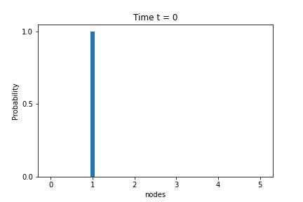
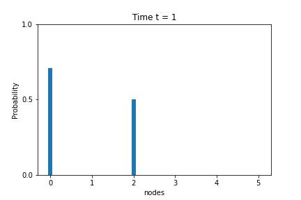
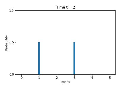
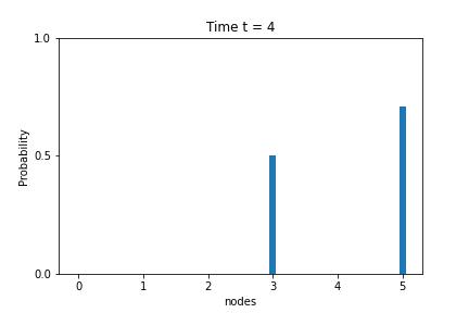
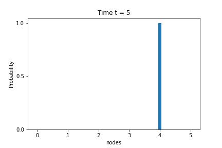
We can visualize the movement of the quantum walker in terms of probability. Suppose the walker starts at vertex $j$ at time $t=0$ with the initial state $\ket{\psi_{j}}$. Probability of getting it at vertex $k$ at time $t$ is Pt​(j,k)=⟨ψk|[S​(2β€‹Ξ βˆ’I)]t|ψj⟩subscriptπ‘ƒπ‘‘π‘—π‘˜quantum-operator-productsubscriptπœ“π‘˜superscriptdelimited-[]𝑆2Π𝐼𝑑subscriptπœ“π‘—P_{t}(j,k)=\braket{\psi_{k}}{[S(2\Pi-I)]^{t}}{\psi_{j}}. Theorem 3 indicates when $0\leq t\leq j$ we have

$$P_{t}(j,k)=\begin{cases}1&~{}\text{when}~{}k=j~{}\text{and}~{}t=0;\\ \frac{1}{2}&~{}\text{when}~{}k=j+t~{}\text{or}~{}k=j-t~{}\text{and}~{}t=0\leq j<j-1;\\ \frac{1}{\sqrt{2}}&~{}\text{when}~{}k=0~{}\text{and}~{}t=j.\end{cases}$$ (25)

When $j+1\leq t\leq n-j-1$ we have

$$P_{t}(j,k)=\begin{cases}\frac{1}{2}&~{}\text{when}~{}k=j+t~{}\text{or}~{}k=t-j~{}\text{and}~{}j+1\leq t<n-j-1;\\ \frac{1}{2}&~{}\text{when}~{}k=n-2j-1~{}\text{and}~{}t=n-j-1;\\ \frac{1}{\sqrt{2}}&~{}\text{when}~{}k=n-1~{}\text{and}~{}t=n-j-1.\end{cases}$$ (26)

Also for $n-j\leq t\leq n-1$ we have

$$P_{t}(j,k)=\begin{cases}\frac{1}{2}&~{}\text{when}~{}k=2n-t-j-2~{}\text{or}~{}k=t-j~{}\text{and}~{}n-j\leq t<n-1;\\ 1&~{}\text{when}~{}k=n-j-1~{}\text{and}~{}t=n-1.\end{cases}$$ (27)

Other than these values of $t,j$ and $k$ we have $P_{t}(j,k)=0$. For example, we consider a path graph with $6$ vertices with a walker who initiates walking at vertex $j=1$. There is a PST between vertex $1$ and $4$. We plot $P_{t}(j,k)$ with bar diagrams for different values of $t$ in figure 1.

Refer to caption
Refer to caption
Refer to caption
Refer to caption
Refer to caption
Figure 1: The probability of getting the walker at the vertex $k\in P_{6}$ at different time instance $t=0,1,\dots 5$. Suppose the walker started at vertex $1$ at $t=0$. At $t=5$, it reaches vertex $4$. Therefore, the probability of getting the walker at time $t=0$ at vertex $1$ is $1$. Similarly, the probability of getting the walker at time $t=5$ at vertex $4$ is $1$. There is a PST between vertices $1$ and $4$ at time $t=5$.

5 Conclusion

In this article, we study PST in the path graphs and the cycle graphs with an arbitrary number of vertices. We consider an alternative approach to PST which is based on the Markovian quantum walk. The idea of the Markovian quantum walk is a variant of the Szegedy quantum walk. In case of the continuous-time quantum walk, we consider $\exp(itA(G))$ as the evolution operator. PST based on the continuous-time quantum walk is limited in path graph with at most $3$ vertices and cycle graph with at most $4$ vertices. Considering the evolution operator S​(2β€‹Ξ βˆ’I)𝑆2Π𝐼S(2\Pi-I) of Markovian quantum walk we overcome this limitation. We investigate the propagation of a quantum walker on path and cycle graphs. In a cycle graph with $2m$ vertices, we establish PST between any pair of vertices $j$ and $j+m$ at time $t=m$ for $j=0,1,\dots m-1$. Also, in case of path graphs $P_{n}$ we observe PST between any pair of vertices $j$ and $n-j-1$ at time $t=n-1$ for $0\leq j<\frac{n-1}{2}$. When $n$ is odd the vertex $\frac{n-1}{2}$ is a periodic vertex. Therefore, this work opens up a new direction to investigate PST in graphs which might be more efficient in quantum communication.

The idea of PST based on Markovian quantum walk is new and different from the other proposals of PST. It is well-known that the antipodal vertices of a hypercube graph allow PST based on the continuous-time quantum walk. In our case, only a two-dimensional hypercube graph which is a cycle graph with four vertices allows PST. Hypercube graphs do not allow PST based on Markovian quantum walk in them when their dimension is more than two. Interestingly, all the vertices in the hypercube graph of dimension 4 are periodic at time $t=12$. The central vertex of the star graphs is periodic at time $t=2$. The non-central vertices of the star graphs are periodic at time $t=4$. Tensor product of two path graphs $P_{i}\otimes P_{j}$ allows PST when $i+j\leq 7$. Computer programs identify these graphs supporting PST or having periodic vertices in them. Here, we mention them without proof, which an interested reader may attempt.

Funding

This work is supported by the SERB funded project entitled β€œTransmission of quantum information using perfect state transfer” (Grant no. CRG/2021/001834).

Appendix

Proof of Lemma 1:

Proof.
(2β€‹Ξ βˆ’I)​|ψj⟩=2​Π​|ψjβŸ©βˆ’|ψj⟩=2​|ψjβŸ©β€‹βŸ¨Οˆj|ψjβŸ©βˆ’|ψj⟩=2​|ψjβŸ©βˆ’|ψj⟩=|ψj⟩orS​(2β€‹Ξ βˆ’I)​|ψj⟩=S​|ψj⟩=12​S​(|j​(j+1)⟩+|j​(jβˆ’1)⟩)=12​(|(j+1)​j⟩+|(jβˆ’1)​j⟩).2Π𝐼ketsubscriptπœ“π‘—2Ξ ketsubscriptπœ“π‘—ketsubscriptπœ“π‘—2ketsubscriptπœ“π‘—inner-productsubscriptπœ“π‘—subscriptπœ“π‘—ketsubscriptπœ“π‘—2ketsubscriptπœ“π‘—ketsubscriptπœ“π‘—ketsubscriptπœ“π‘—or𝑆2Π𝐼ketsubscriptπœ“π‘—π‘†ketsubscriptπœ“π‘—12𝑆ket𝑗𝑗1ket𝑗𝑗112ket𝑗1𝑗ket𝑗1𝑗\begin{split}&(2\Pi-I)\ket{\psi_{j}}=2\Pi\ket{\psi_{j}}-\ket{\psi_{j}}=2\ket{\psi_{j}}\braket{\psi_{j}}{\psi_{j}}-\ket{\psi_{j}}=2\ket{\psi_{j}}-\ket{\psi_{j}}=\ket{\psi_{j}}\\ \text{or}~{}&S(2\Pi-I)\ket{\psi_{j}}=S\ket{\psi_{j}}=\frac{1}{\sqrt{2}}S(\ket{j(j+1)}+\ket{j(j-1)})=\frac{1}{\sqrt{2}}(\ket{(j+1)j}+\ket{(j-1)j}).\end{split} (28)

∎

Proof of Lemma 2:

Proof.
(2β€‹Ξ βˆ’I)​|(j+1)​j⟩=2​Π​|(j+1)​jβŸ©βˆ’I​|(j+1)​j⟩=2​|ψ(j+1)βŸ©β€‹βŸ¨Οˆ(j+1)|(j+1)​jβŸ©βˆ’|(j+1)​j⟩=2​12​|ψ(j+1)βŸ©βˆ’|(j+1)​j⟩,2Π𝐼ket𝑗1𝑗2Ξ ket𝑗1𝑗𝐼ket𝑗1𝑗2ketsubscriptπœ“π‘—1inner-productsubscriptπœ“π‘—1𝑗1𝑗ket𝑗1𝑗212ketsubscriptπœ“π‘—1ket𝑗1𝑗\begin{split}(2\Pi-I)\ket{(j+1)j}&=2\Pi\ket{(j+1)j}-I\ket{(j+1)j}=2\ket{\psi_{(j+1)}}\braket{\psi_{(j+1)}}{(j+1)j}-\ket{(j+1)j}\\ &=2\frac{1}{\sqrt{2}}\ket{\psi_{(j+1)}}-\ket{(j+1)j},\end{split} (29)

since $\braket{\psi_{(j+1)}}{(j+1)j}=\frac{1}{\sqrt{2}}$. Applying equation (2) we have

S​(2β€‹Ξ βˆ’I)​|(j+1)​j⟩=S​(2​12​12​(|(j+1)​(j+2)⟩+|(j+1)​j⟩)βˆ’|(j+1)​j⟩)=S​(|(j+1)​(j+2)⟩+|(j+1)​jβŸ©βˆ’|(j+1)​j⟩)=S​|(j+1)​(j+2)⟩=|(j+2)​(j+1)⟩.𝑆2Π𝐼ket𝑗1𝑗𝑆21212ket𝑗1𝑗2ket𝑗1𝑗ket𝑗1𝑗𝑆ket𝑗1𝑗2ket𝑗1𝑗ket𝑗1𝑗𝑆ket𝑗1𝑗2ket𝑗2𝑗1\begin{split}S(2\Pi-I)\ket{(j+1)j}&=S\left(2\frac{1}{\sqrt{2}}\frac{1}{\sqrt{2}}(\ket{(j+1)(j+2)}+\ket{(j+1)j})-\ket{(j+1)j}\right)\\ &=S\left(\ket{(j+1)(j+2)}+\ket{(j+1)j}-\ket{(j+1)j}\right)=S\ket{(j+1)(j+2)}=\ket{(j+2)(j+1)}.\end{split} (30)

∎

Proof of Lemma 3:

Proof.
(2β€‹Ξ βˆ’I)​|(jβˆ’1)​j⟩=2​Π​|(jβˆ’1)​jβŸ©βˆ’|(jβˆ’1)​j⟩=2​|ψ(jβˆ’1)βŸ©β€‹βŸ¨Οˆ(jβˆ’1)|(jβˆ’1)​jβŸ©βˆ’|(jβˆ’1)​j⟩=2​12​|ψ(jβˆ’1)βŸ©βˆ’|(jβˆ’1)​j⟩,2Π𝐼ket𝑗1𝑗2Ξ ket𝑗1𝑗ket𝑗1𝑗2ketsubscriptπœ“π‘—1inner-productsubscriptπœ“π‘—1𝑗1𝑗ket𝑗1𝑗212ketsubscriptπœ“π‘—1ket𝑗1𝑗\begin{split}(2\Pi-I)\ket{(j-1)j}&=2\Pi\ket{(j-1)j}-\ket{(j-1)j}=2\ket{\psi_{(j-1)}}\braket{\psi_{(j-1)}}{(j-1)j}-\ket{(j-1)j}\\ &=2\frac{1}{\sqrt{2}}\ket{\psi_{(j-1)}}-\ket{(j-1)j},\end{split} (31)

since $\braket{\psi_{(j-1)}}{(j-1)j}=\frac{1}{\sqrt{2}}$. Applying equation (2) we have

S​(2β€‹Ξ βˆ’I)​|(jβˆ’1)​j⟩=S​(2​12​12​(|(jβˆ’1)​j⟩+|(jβˆ’1)​(jβˆ’2)⟩)βˆ’|(jβˆ’1)​j⟩)=S​(|(jβˆ’1)​(jβˆ’2)⟩+|(jβˆ’1)​jβŸ©βˆ’|(jβˆ’1)​j⟩)=S​|(jβˆ’1)​(jβˆ’2)⟩=|(jβˆ’2)​(jβˆ’1)⟩.𝑆2Π𝐼ket𝑗1𝑗𝑆21212ket𝑗1𝑗ket𝑗1𝑗2ket𝑗1𝑗𝑆ket𝑗1𝑗2ket𝑗1𝑗ket𝑗1𝑗𝑆ket𝑗1𝑗2ket𝑗2𝑗1\begin{split}S(2\Pi-I)\ket{(j-1)j}&=S\left(2\frac{1}{\sqrt{2}}\frac{1}{\sqrt{2}}(\ket{(j-1)j}+\ket{(j-1)(j-2)})-\ket{(j-1)j}\right)\\ &=S\left(\ket{(j-1)(j-2)}+\ket{(j-1)j}-\ket{(j-1)j}\right)=S\ket{(j-1)(j-2)}=\ket{(j-2)(j-1)}.\end{split} (32)

∎

References