Censoring heavy-tail count distributions for parameters estimation with an application to stable distributions

Abstract

Some families of count distributions do not have a closed form of the probability mass function and/or finite moments and therefore parameter estimation can not be performed with the classical methods. When the probability generating function of the distribution is available, a new approach based on censoring and moment criterion is introduced, where the original distribution is replaced with that censored by using a Geometric distribution. Consistency and asymptotic normality of the resulting estimators are proven under suitable conditions. The crucial issue of selecting the censoring parameter is addressed by means of a data-driven procedure. Finally, this novel approach is applied to the discrete stable family and the finite sample performance of the estimators is assessed by means of a Monte Carlo simulation study.

and

1 Introduction

Heavy-tailed count data naturally arise in many applied disciplines, such as actuarial science, medicine, biology, computer science, economics and environmental science among many others (see e.g., El-Shaarawi et al., 2011, Edwards et al., 2016, Sun al., 2021). A plethora of family of distributions has been proposed in literature to model heavy-tailed count data, but, unfortunately, the use of some of them is inhibited by the lack of an explicit, or easily computable, expression for their probability mass function (p.m.f.) and by the lack of any-order moments for all or some parameters values. Obviously, in these cases, the use of standard maximum-likelihood or moment-based estimation is precluded.

We propose a very general procedure, based on censoring, which requires only the knowledge of the probability generating function (p.g.f.) and allows to estimate the distribution parameters also when a closed-form of the p.m.f. and/or moments do not exist. One of its appealing characteristics is that parameters estimation is performed by means of a suitably modified moment-based technique, which is appropriate even for distributions without moments. Indeed, the censored count distribution still depends on the parameters of the original one but, having finite moments, allows the application of a moment-based method. Obviously, the choice of the censoring parameter introduces a source of arbitrariness, which can be reduced by adopting data-driven selection criteria. We focus on two-parameters family of distributions and prove that resulting estimators are consistent and have an asymptotic normal distribution under rather general mathematical conditions. These results can be extended to families with $k>2$ parameters under analogous conditions.

It is worth noting that the censoring operation has been already considered by Zhu and Harry (2009) for modeling different tail heaviness. More precisely, censoring has been used to generalize the Poisson-inverse Gaussian distribution to a more flexible three-parameter family, including, as boundary cases, the Poisson and the discrete stable distributions. The family of discrete stable distributions, introduced by Steutel and van Harn (1979), is large and flexible, allowing skewness, heavy tails, overdispersion, and have many intriguing mathematical properties (see e.g. Christoph et al., 1998, Devroye, 1993). However, the lack of a closed form expression for the p.m.f. and the non-existence of moments for some parameters values have been a major drawback to its use by practitioners. Some attempts for parameter estimation have been performed by Kemp et al. (1988), Marcheselli et al. (2008), Doray et al. (2009) and Zhu and Harry (2009) among others. The application of the novel estimation procedure based on censoring to this family gives rise to estimators which have a closed and simple expression and are consistent and asymptotically normal. Moreover, they show a really satisfactory performance for moderate sample size, also when the parameters are in a neighborhood of the boundary values ensuring the existence of moments.

The general procedure is illustrated in Section 2 and results on the discrete stable distributions are given in Section 3. A simulation study is presented in Section 4 while Section 5 is devoted to concluding remarks. All the proofs are reported in the Appendix.

2 Parameter estimation by censoring

Let $X$ be a count random variable, i.e. a random variable (r.v.) with values in $\mathbb{N}_{0}=\{0,1,2,\dots\}$ such that $\operatorname{E}[X]$ is not necessarily finite. Moreover, denote by $g$ the probability generating function (p.g.f.) of $X$, namely $g(s)=\operatorname{E}[s^{X}]$ for any $s\in[0,1]$.

When $X$ does not have finite moments and the p.m.f. has no closed-form, any inference procedure becomes cumbersome. To address parameters estimation, we propose an original and effective approach based on a stochastic perturbation of $X$, giving rise to a censored r.v. with finite moments. More precisely, let $T_{p}$ be a Geometric r.v. with parameter $p\in]0,1]$ and p.m.f.

$$h(n)=P(T_{p}=n)=p(1-p)^{n-1},\quad n\geq 1$$

and let

$$Y=X\mathbf{1}_{\{X<T_{p}\}}$$

be the $p$-censoring of $X$. It is worth noting that $\operatorname{E}[Y]$ is finite since

$$\operatorname{E}[Y]\leq\operatorname{E}[T_{p}-1]={{1-p}\over{p}}.$$

Moreover, the p.g.f. of $Y$ can be expressed as a function of the p.g.f. of $X$.

Proposition 1.

Let $g_{Y}$ be the p.g.f of $Y$. For any $s\in[0,1]$,

$$g_{Y}(s)=1-g(1-p)+g(s(1-p)).$$ (1)

In particular,

$$\operatorname{E}[Y]=(1-p)g^{\prime}(1-p),\qquad\operatorname{E}[Y^{2}]=(1-p)^{2}g^{\prime\prime}(1-p)+(1-p)g^{\prime}(1-p).$$ (2)

Now suppose that the distribution of $X$ depends on two parameters $\theta_{1},\theta_{2}$ which can be written as

$$\theta_{1}=f_{1}(p,g(1-p),\operatorname{E}[Y]),\quad\theta_{2}=f_{2}(p,g(1-p),\theta_{1}),$$ (3)

where $f_{1}$, $f_{2}$ are two (known) suitable differentiable functions. Condition (3) is not very restrictive and is verified for large classes of distributions, such as discrete stable distributions. In order to estimate $\theta_{1}$ and $\theta_{2}$, consider a random sample $(X_{1},\dots,X_{n})$, with $X_{i}\sim X$ for $i=1,\ldots,n$, and $n$ Geometric independent r.v.s $(T_{p,1},\dots,T_{p,n})$ with parameter $p$, independent of $(X_{1},\dots,X_{n})$, and let

$$\widehat{m}_{p,1}=n^{-1}\sum_{i=1}^{n}X_{i}\mathbf{1}_{\{X_{i}<T_{p,i}\}},\qquad\widehat{g}(1-p)=n^{-1}\sum_{i=1}^{n}(1-p)^{X_{i}}$$ (4)

be the empirical first-order moment of the $p$-censoring of $X$ and the empirical probability generating function of $X$ computed at $1-p$, respectively. The most trivial estimators of $\theta_{1}$ and $\theta_{2}$ could be obtained by means of the plug-in technique by replacing $\operatorname{E}[Y]$, that is the finite moment of the $p$-censoring r.v., with its empirical counterpart. Obviously, the variability of the plug-in estimators is inflated by the randomness introduced by censoring. On the other hand, a more precise estimator of $\theta_{1}$ is provided by considering the conditional expectation of the plug-in estimator given the random sample. Therefore, the proposed estimators are given by

$$\widehat{\theta}_{1}=\operatorname{E}[f_{1}(p,\widehat{g}(1-p),\widehat{m}_{p,1})|X_{1},\ldots,X_{n}],\quad\widehat{\theta}_{2}=f_{2}(p,\widehat{g}(1-p),\widehat{\theta}_{1}).$$

It must be pointed out that, if a closed form expression for $\widehat{\theta}_{1}$ does not exist, it can be approximated by considering $R$ independent generations of $n$ independent Geometric r.v.s with parameter $p$, $(T_{p,1,r},\dots,T_{p,n,r})$, giving rise to $R$ empirical first-order moments $\widehat{m}_{p,1,r}$ ($r=1,\ldots,R)$ in such a way that $\widehat{\theta}_{1}$ can be obtained as ${1/R}\sum_{r=1}^{R}f_{1}(p,\widehat{g}(1-p),\widehat{m}_{p,1,r})$. Obviously, the choice of $R$ is under the control of the researcher and, owing to the negligible computational effort, can be taken large enough to ensure an excellent approximation.

Introducing the $p$-censoring r.v. $Y$ induces a source of arbitrariness due to choice of the censoring parameter $p$. Indeed, $\widehat{\theta}_{1}$ and $\widehat{\theta}_{2}$ constitute a family of estimators indexed by $p$ and, therefore, the selection of the parameter $p$ ensuring enough information on the tail of $X$ and good performance of the corresponding estimators is crucial. In general, values of $p$ in $]0,1/2]$ are advisable. A reasonable approach is to consider a data-driven procedure which should be guided by the features of the p.g.f. of $X$. Then, once the suitable r.v. $p_{*}$ depending on $X_{1},\ldots,X_{n}$ is defined, the following estimators can be considered

$$\widehat{\theta}_{1}^{*}=\operatorname{E}[f_{1}(p_{*},\widehat{g}(1-p_{*}),\widehat{m}_{p_{*},1})|X_{1},\ldots,X_{n}],\quad\widehat{\theta}_{2}^{*}=f_{2}(p_{*},\widehat{g}(1-p_{*}),\widehat{\theta}_{1}^{*}).$$ (5)

It must be pointed out that, whatever data-driven criterion is adopted, under rather mild conditions on $p_{*}$, thanks to $\eqref{stime_con_p*}$ and to the Delta method, the asymptotic consistency and normality of $\widehat{\theta}_{1}^{*}$ and $\widehat{\theta}_{2}^{*}$ can be proven.

Proposition 2.

Suppose there exist $p\in\,]0,1/2]$ and a sequence $(Z_{n})_{n}$ of independent and identically distributed r.v.s, with $\operatorname{E}[Z_{1}^{2}]<\infty$, such that

$$(p_{*}-p)-{{\sum_{i=1}^{n}(Z_{i}-\operatorname{E}[Z_{1}])}\over{n}}=o(1)\quad a.s$$ (6)

and $\sqrt{n}o(1)=o_{P}(1)$, where $o_{P}(1)$ denotes a r.v. which goes to 0 in probability. Moreover, suppose ${{\partial f_{1}}\over{\partial z}}$ is a bounded function.

Then $\widehat{\theta}_{1}^{*}$ and $\widehat{\theta}_{2}^{*}$ converge to $\theta_{1}$ and $\theta_{2}$ almost surely and $[\sqrt{n}(\widehat{\theta}_{1}^{*}-\theta_{1}),\sqrt{n}(\widehat{\theta}_{2}^{*}-\theta_{2})]$ converges in distribution to ${\mathcal{N}}(0,\Sigma)$, where $\Sigma$ is the variance-covariance matrix of $[W_{1},W_{2}]$, with

$$W_{1}={{\partial f_{1}}\over{\partial x}}(P_{0})Z_{1}+{{\partial f_{1}}\over{\partial y}}(P_{0})X^{\prime}_{1}+{{\partial f_{1}}\over{\partial z}}(P_{0})X^{\prime\prime}_{1},$$

$$W_{2}=({{\partial f_{2}}\over{\partial x}}(P_{1})+{{\partial f_{2}}\over{\partial z}}(P_{1}){{\partial f_{1}}\over{\partial x}}(P_{0}))Z_{1}\\ +({{\partial f_{2}}\over{\partial y}}(P_{1})+{{\partial f_{2}}\over{\partial z}}(P_{1}){{\partial f_{1}}\over{\partial y}}(P_{0}))X^{\prime}_{1}+{{\partial f_{2}}\over{\partial z}}(P_{1}){{\partial f_{1}}\over{\partial z}}(P_{0})X^{\prime\prime}_{1}$$

and

$$X^{\prime}_{1}=(1-p)^{X_{1}}-\operatorname{E}[X_{1}(1-p)^{X_{1}-1}]Z_{1},\ \ X^{\prime\prime}_{1}=X_{1}(1-p)^{X_{1}}-\operatorname{E}[X_{1}^{2}(1-p)^{X_{1}-1}]Z_{1},$$ (7)

$$P_{0}=(p,g(p),\operatorname{E}[X_{1}(1-p)^{X_{1}}]),\ \ P_{1}=(p,g(p),\theta_{1}).$$

It should be noted that (6) essentially requires that the selected data-driven criterion ensures the existence of a constant $p\in\,]0,1/2]$ such that the sequence $(p_{*}-p)_{n}$ is asymptotically equivalent to a sequence of averages of i.i.d. centered r.v.s. In the following Section, a data-driven procedure giving rise to $p_{*}$, which satisfies such condition, will be introduced for the discrete stable family. Moreover, when the parameter of the Geometric r.v. is not selected using a data-driven procedure but it is fixed in advance, the consistency and the asymptotic normal distribution of $[\widehat{\theta}_{1},\widehat{\theta}_{2}]$ hold under the sole assumption that ${{\partial f_{1}}\over{\partial z}}$ is bounded.

As to the estimation of $\Sigma$, a suitable estimator is given by the sample variance-covariance matrix of $[W_{1,1}^{*},W_{2,1}^{*}],\ldots,[W_{1,n}^{*},W_{2,n}^{*}]$, where

$$W_{1,i}^{*}={{\partial f_{1}}\over{\partial x}}(P^{*}_{0})Z_{i}+{{\partial f_{1}}\over{\partial y}}(P^{*}_{0})X^{\prime}_{i}+{{\partial f_{1}}\over{\partial z}}(P^{*}_{0})X^{\prime\prime}_{i},$$

$$W_{2,i}^{*}=({{\partial f_{2}}\over{\partial x}}(P_{1}^{*})+{{\partial f_{2}}\over{\partial z}}(P_{1}^{*}){{\partial f_{1}}\over{\partial x}}(P_{0}^{*}))Z_{i}\\ +({{\partial f_{2}}\over{\partial y}}(P^{*}_{1})+{{\partial f_{2}}\over{\partial z}}(P^{*}_{1}){{\partial f_{1}}\over{\partial y}}(P^{*}_{0}))X^{\prime}_{i}+{{\partial f_{2}}\over{\partial z}}(P^{*}_{1}){{\partial f_{1}}\over{\partial z}}(P^{*}_{0})X^{\prime\prime}_{i},$$

$P^{*}_{0}=(p_{*},\widehat{g}(p_{*}),\widehat{m}_{p_{*},1})$, $P^{*}_{1}=(p_{*},\widehat{g}(p_{*}),\widehat{\theta}_{1}^{*})$ and $X^{\prime}_{i}$, $X^{\prime\prime}_{i}$ have expressions analogous to those reported in (7). Indeed, under the assumptions of the previous proposition, $P^{*}_{0}$, $P^{*}_{1}$ converge almost surely to $P_{0},P_{1}$ and therefore the sample variance-covariance matrix is a consistent estimator of $\Sigma$.

3 Parameter estimation for the discrete stable family

The discrete stable family, denoted as $\mathcal{DS}(a,\lambda)$ with $a\in\,]0,1]$ and $\lambda>0$, constitutes an interesting two-parameter model of count distributions on $\mathbb{N}_{0}$ with a Paretian tail, whose use is inhibited by the lack of an explicit expression for its p.m.f. and of moments of any order when $a<1$. Indeed, these features preclude the exploitation of the maximum-likelihood or the moment method for parameter estimation. However, since its p.g.f. is available in a simple form, the proposed censoring technique can be suitably applied. In particular, the p.g.f. is given by

$$g(s)=\exp\left(-\lambda(1-s)^{a}\right)$$ (8)

and, obviously, for $a=1$ the discrete stable family reduces to the Poisson family of distributions and $\operatorname{E}[X]=\infty$ when $a<1$. Now, let $X_{1},\dots,X_{n}$ be a random sample from $X\sim\mathcal{DS}(a,\lambda)$. By using (1), the p.g.f of the $p$-censoring turns out to be

$$g_{Y}(s)=1-e^{-\lambda p^{a}}+e^{-\lambda(1-s(1-p))^{a}},$$

in such a way that

$$\operatorname{E}[Y]=g(1-p)p^{a-1}(1-p)\lambda a$$ (9)

and, by noting that $g(1-p)=\exp\left(-\lambda p^{a}\right)$,

$$\operatorname{E}[Y]=-ap^{-1}(1-p)g(1-p)\log(g(1-p)).$$ (10)

From (10) and (9), it is at once apparent that the parameters $a$ and $\lambda$ can be expressed as in (2) and thus, from (5), they can be estimated by means of

$$\widehat{a} =-\operatorname{E}[{{p_{*}\widehat{m}_{p_{*},1}}\over{(1-p_{*})\widehat{g}(1-p_{*})\,\log\big{(}\widehat{g}(1-p_{*})\big{)}}}|X_{1},\ldots,X_{n}]={{p_{*}\operatorname{E}[m_{p_{*},1}|X_{1},\ldots,X_{n}]}\over{(1-p_{*})\widehat{g}(1-p_{*})\,\log\big{(}\widehat{g}(1-p_{*})\big{)}}}$$

$$=-{{p_{*}}\over{(1-p_{*})\widehat{g}(1-p_{*})\,\log\big{(}\widehat{g}(1-p_{*})\big{)}}}n^{-1}\sum_{i=1}^{n}X_{i}(1-p_{*})^{X_{i}}$$ (11)

and

$$\widehat{\lambda}=-p_{*}^{-\widehat{a}}\log\big{(}\widehat{g}(1-p_{*})\big{)},$$ (12)

where $p_{*}$, representing the data-driven choice of the censoring parameter, depends only on $X_{1},\ldots,X_{n}$.

In order to ensure satisfactory finite sample performance of estimators $\eqref{estimator_a}$ and (12), the data-driven choice of $p_{*}$ is crucial. In particular, $p*$ should be chosen to provide that the denominator in (3) is not too close to zero. Then, since $p_{*}$ is less or equal to $1/2$ and $x\mapsto-x\log x$ has maximum at $x=1/e$, we propose the following data-driven criterion

$$p_{*}={\rm argmax}_{p\in]0,1/2]}\{-\widehat{g}(1-p)\log\big{(}\widehat{g}(1-p)\big{)}\}=\max\{p\in]0,1/2]:\widehat{g}(1-p)\geq 1/e\}.$$ (13)

Note that if $\widehat{g}(1/2)\geq 1/e$, $p_{*}=1/2$ and (3) reduces to

$$\widehat{a}=-{{n^{-1}\sum_{i=1}^{n}X_{i}2^{-X_{i}}}\over{\widehat{g}(1/2)\,\log\big{(}\widehat{g}(1/2)\big{)}}}$$

while if $\widehat{g}(1/2)<1/e$, $p_{*}$ is less than $1/2$ and such that $\widehat{g}(1-p)=1/e$ and the estimator of $a$ is given by

$$\widehat{a}={{ep_{*}n^{-1}\sum_{i=1}^{n}X_{i}(1-p_{*})^{X_{i}}}\over{1-p_{*}}}.$$

Then, the estimators for $a$ and $\lambda$ turn out to be

$$\widehat{a}={{ep_{*}n^{-1}\sum_{i=1}^{n}X_{i}(1-p_{*})^{X_{i}}}\over{1-p_{*}}}\mathbf{1}_{\{p_{*}<1/2\}}-{{n^{-1}\sum_{i=1}^{n}X_{i}2^{-X_{i}}}\over{\widehat{g}(1/2)\,\log\big{(}\widehat{g}(1/2)\big{)}}}\mathbf{1}_{\{p_{*}=1/2\}}$$ (14)

and

$$\widehat{\lambda}=p_{*}^{-\widehat{a}}\mathbf{1}_{\{p_{*}<1/2\}}-2^{\,\widehat{a}}\log\big{(}\widehat{g}(1/2)\big{)}\mathbf{1}_{\{p_{*}=1/2\}}.$$ (15)

It is worth noting that asymptotically $p_{*}<1/2$ almost surely when $\lambda>2^{a}$, otherwise $p_{*}=1/2$ if $\lambda<2^{a}$.

Proposition 3.

$p_{*}$ converges almost surely to $p=\min(\lambda^{-1/a},1/2)$. Moreover, for $\lambda>2^{a}$ condition $(6)$ holds with $Z_{i}=e\lambda^{-1/a}(1-\lambda^{-1/a})^{X_{i}}/a$ while, for $\lambda<2^{a}$, with $Z_{1}=0$.

By using Proposition 2 and Proposition 3, consistency and asymptotic normality of estimators $\widehat{a},\,\widehat{\lambda}$ are obtained.

Corollary 1.

$\widehat{a},$ $\widehat{\lambda}$ converge almost surely to $a,\lambda$ for large $n$ and $[\sqrt{n}(\widehat{a}-a),\sqrt{n}(\widehat{\lambda}-\lambda)]$ converges in distribution to ${\mathcal{N}}(0,\Sigma)$, where $\Sigma$ is the variance-covariance matrix of $[W_{1},W_{2}]$, with

$$W_{1}=e\lambda^{-1/a}X_{1}(1-\lambda^{-1/a})^{X_{1}-1},$$

$$W_{2}=-e\lambda\big{(}(1-\lambda^{-1/a})^{X_{1}}-a^{-1}(\lambda^{-1/a}\log{\lambda})X_{1}(1-\lambda^{-1/a})^{X_{1}-1}\big{)}$$

for $\lambda>2^{a}$ while

$$W_{1}=\lambda^{-1}2^{a}e^{{\lambda}\over{2^{a}}}(X_{1}2^{-X_{1}}+a(1-\lambda 2^{-a})2^{-X_{1}}),$$

$$W_{2}=2^{a}e^{{\lambda}\over{2^{a}}}(X_{1}2^{-X_{1}}\log 2+\big{(}a(1-\lambda 2^{-a})\log 2-1\big{)}2^{-X_{1}})$$

for $\lambda<2^{a}$.

As in the general case introduced in Section 2, a suitable estimator of $\Sigma$ is given by the sample variance-covariance matrix of $[W_{1,1}^{*},W_{2,1}^{*}],\ldots,[W_{1,n}^{*},W_{2,n}^{*}]$, where

$$W_{1,i}^{*}=ep_{*}X_{i}(1-p_{*})^{X_{i}-1},\qquad W_{2,i}^{*}=-e{\widehat{\lambda}}\big{(}(1-p_{*})^{X_{i}}+{X_{i}(1-p_{*})^{X_{i}-1}}p_{*}\log{p_{*}}\big{)}$$

for $p_{*}<1/2$ while

$$W_{1,i}^{*}=-{{2^{-X_{1}}\big{(}X_{1}+\widehat{a}(1+\log\widehat{g}(1/2))\big{)}}\over{\widehat{g}(1/2)\log\widehat{g}(1/2)}},\ \ W_{2}=2^{\widehat{a}-X_{1}}e^{{\widehat{\lambda}}\over{2^{\widehat{a}}}}\big{(}X_{1}\log 2+\big{(}\widehat{a}(1-\widehat{\lambda}2^{-\widehat{a}})\log 2-1\big{)}\big{)}$$

for $p_{*}=1/2$.

4 Simulation study

The performance of the estimators (14) and (15) was assessed by means of an extensive Monte Carlo simulation implemented by using R (R Core Team, 2020). The realizations of the discrete stable distribution were generated by using the following equality in law (Devroye, 1993)

$$\mathcal{DS}(a,\lambda)\overset{\mathcal{L}}{=}\mathcal{P}(\mathcal{PS}(a,\lambda)),$$

where $\mathcal{P}$ denotes the Poisson distribution and $\mathcal{PS}$ denotes the Positive Stable distribution. For generating realizations from the Positive Stable distribution, the classical Kanter’s representation (Kanter, 1975)

$$\mathcal{PS}(a,\lambda)\overset{\mathcal{L}}{=}\Big{(}\frac{\sin((1-a)\pi\mathcal{U})}{\mathcal{G}(1,1)\sin(a\pi\mathcal{U})}\Big{)}^{(1-a)/a}\Big{(}\frac{\lambda\sin(a\pi\mathcal{U})}{\sin(\pi\mathcal{U})}\Big{)}^{1/a}$$

was adopted, where $\mathcal{G}$ and $\mathcal{U}$ are the Gamma and the standard Uniform distribution, respectively. As to the parameter values, the value of $a$ was set equal to $0.25,0.5,0.75,1$ while all the values varying from $0.5$ to $12$ by $0.5$ were considered for $\lambda$.

For each combination of $a$ and $\lambda$ values, $5000$ samples of size $n=100,200$ were independently generated from $\mathcal{DS}(a,\lambda)$. For each sample, first the censoring parameter was selected according to (13) and then parameter estimates were obtained by means of (14) and (15), together with the corresponding variance estimates. Moreover, confidence interval estimates for $a$ and $\lambda$ at confidence level $1-\alpha=0.95$ were obtained using the quantiles of the standard normal distribution. From the Monte Carlo distributions, the Relative Root Mean Squared Error (RRMSE) of (14) and (15) was obtained and reported in Table 1 and Table 2, respectively. For any combination of $\lambda$ and $a$, the RRMSEs of both estimators are rather satisfactory and obviously decrease as $n$ increases. Moreover, for any fixed $n$ and $a$, the RRMSE of $\widehat{a}$ decreases as $\lambda$ increases. Similarly, for any fixed $n$ and $\lambda$, the RRMSE of $\widehat{\lambda}$ decreases as $a$ increases for the larger values of $\lambda$.

Finally, the empirical coverages of the confidence intervals were computed. For any fixed value $a=0.25,0.5,0.75,1$, Figure 1 depicts the empirical coverage of the 0.95 confidence intervals for $\lambda$ varying from $0.5$ to $12$ by $0.5$ both for $n=100$ and $n=200$. Analogously, Figure 2 depicts the empirical coverage of the 0.95 confidence intervals for $a$ when $\lambda$ varies from $0.5$ to $12$ by $0.5$. From Figures 1 and 2 it is at once apparent that the empirical coverages are really satisfactory for both parameters even for $n=100$. Empirical coverages of the confidence intervals for $a$ are less close to $0.95$ only when $a=1$ and $n=100$, while for $n=200$ they approach the nominal one.

Table 1: Percentage values of the RRMSE of $\widehat{a}$ for various combinations of $\lambda$ values, $a$ values and sample sizes.

	$a=0.25$		$a=0.5$		$a=0.75$		$a=1$
$\lambda$	$n=100$	$n=200$	$n=100$	$n=200$	$n=100$	$n=200$	$n={100}$	$n={200}$
$0.5$	23	16	15	10	10	7	4	3
$1$	20	14	12	9	8	6	4	3
$2$	14	10	9	7	7	5	5	3
$5$	13	10	8	5	5	3	2	1
$10$	14	9	7	5	4	3	1	1

Table 2: Percentage values of the RRMSE of $\widehat{\lambda}$ for various combinations of $\lambda$ values, $a$ values and sample sizes.

	$a=0.25$		$a=0.5$		$a=0.75$		$a=1$
$\lambda$	$n=100$	$n=200$	$n=100$	$n=200$	$n=100$	$n=200$	$n={100}$	$n={200}$
$0.5$	16	11	16	11	16	11	16	11
$1$	13	9	13	9	13	9	12	8
$2$	14	10	11	8	10	7	10	7
$5$	25	16	13	9	8	6	6	4
$10$	36	23	17	11	9	6	4	3

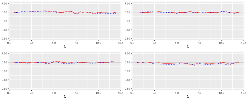
Figure 1: Empirical coverage of 95% confidence intervals for ${\lambda}$ with $n=100$ (dashed line) and $n=200$ (solid line). Top-left: $a=0.25$, top-right: $a=0.5$, bottom-left: $a=0.75$, bottom-right: $a=1$.

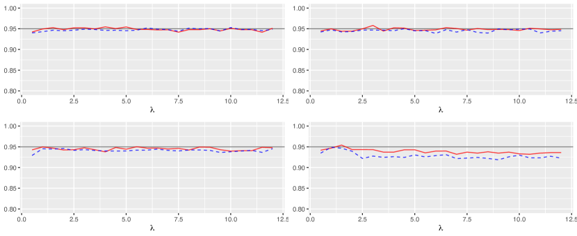
Figure 2: Empirical coverage of 95% confidence intervals for ${a}$ with $n=100$ (dashed line) and $n=200$ (solid line). Top-left: $a=0.25$, top-right: $a=0.5$, bottom-left: $a=0.75$, bottom-right: $a=1$.

5 Discussion

The use of some family of count distributions, particularly suitable for modelling heavy-tailed count data, is precluded by the lack of an explicit, or easily computable, expression for their p.m.f. and by the lack of any-order moments at least for some parameters values. In these cases, a general procedure for parameter estimation is welcomed and, even more so, if it allows to obtain consistent and asymptotically normal estimators. The proposed procedure, under mild mathematical conditions, not only gives rise to estimators sharing these properties, but also to variance estimators which avoid computationally intensive resampling methods. For the discrete stable family, the proposed estimators also show rather satisfactory performance for finite sample, in terms of coverages of confidence intervals and of relative root mean squared errors. The novel estimation procedure has been introduced referring to distributions depending on two parameters, but it could be generalized to distributions with more parameters. Obviously, when $k$ parameters are under estimation, generally moments up to the order $k-1$ for the $p$-censoring r.v. are involved and they can be straightforwardly obtained by means of Proposition 1.

Finally, further research will be devoted to investigate if the censoring could also be used to introduce a general goodness-of-fit test for count distributions (also without any moments) as few proposals are available and many of them, being tailored to deal with particular distributions, are of limited applicability.

Appendix A Proof of Proposition 1

Since $P(T_{p}\leq n)=1-(1-p)^{n}$, for $n\geq 1$ it holds

$$P(Y=n)=P(X=n)P(T_{p}>n)=P(X=n)(1-p)^{n}.$$

Moreover, it must be pointed out that

$$g(1-p)=\sum_{n=0}^{\infty}(1-p)^{n}P(X=n)=P(T_{p}>X).$$ (16)

Thus

$$g_{Y}(s) =\sum_{n=0}^{\infty}s^{n}P(Y=n)=P(Y=0)+\sum_{n=1}^{\infty}s^{n}(1-p)^{n}P(X=n)$$

$$=P(Y=0)-P(X=0)+g\big{(}s(1-p)\big{)}=P(T_{p}\leq X)+g\big{(}s(1-p)\big{)}$$

$$=1-g(1-p)+g\big{(}s(1-p)\big{)}.$$

From the previous expression, it is at once apparent that $\operatorname{E}[Y]=g^{\prime}_{Y}(1)=(1-p)g^{\prime}(1-p)$ and

$$\operatorname{E}[Y^{2}]=g^{\prime\prime}_{Y}(1)+\operatorname{E}[Y]=(1-p)^{2}g^{\prime\prime}(1-p)+(1-p)g^{\prime}(1-p).$$

Appendix B Proof of Proposition 2

Let $L$ be a constant such that $|{{\partial f_{1}}\over{\partial z}}|\leq L$. Since

$$\Big{|}\widehat{\theta}_{1}^{*}-f_{1}(p_{*},\widehat{g}(1-p_{*}),n^{-1}\sum_{i=1}^{n}X_{i}(1-p_{*})^{X_{i}})\Big{|}\leq L\operatorname{E}[(\widehat{m}_{p_{*},1}-n^{-1}\sum_{i=1}^{n}X_{i}(1-p_{*})^{X_{i}})^{2}|X_{1},\ldots,X_{n}]^{1\over 2}$$

and

$$\operatorname{E}[(\widehat{m}_{p_{*},1}-n^{-1}\sum_{i=1}^{n}X_{i}(1-p_{*})^{X_{i}})^{2}|X_{1},\ldots,X_{n}] =n^{-2}\sum_{i=1}^{n}X_{i}^{2}(1-p_{*})^{X_{i}}\big{(}1-(1-p_{*})^{X_{i}}\big{)}$$

$$=O(1/n)\quad a.s.,$$

the consistency of $\widehat{\theta}_{1}^{*}$ and, consequently, of $\widehat{\theta}_{2}^{*}$ is obtained if

$$\lim_{n}f_{1}(p_{*},\widehat{g}(1-p_{*}),n^{-1}\sum_{i=1}^{n}X_{i}(1-p_{*})^{X_{i}})=\theta_{1}\quad a.s.$$

holds. In other words, thanks to continuity of $f_{1}$ and to condition (6), which implies $\lim_{n}p_{*}=p$ almost surely, it suffices to prove

$$\lim_{n}\widehat{g}(1-p_{*})=g(1-p),\qquad\lim_{n}n^{-1}\sum_{i=1}^{n}X_{i}(1-p_{*})^{X_{i}}=\operatorname{E}[X_{1}(1-p)^{X_{1}}]\qquad a.s.$$

From the Strong Law of Large Numbers and from

$$|(1-p_{*})^{X_{i}}-(1-p)^{X_{i}}|\leq X_{i}2^{1-X_{i}}|p_{*}-p|,$$ (17)

the previous relations, and then the consistency, immediately follow.

Moreover, from (6) and (17), by applying again the Strong Law of Large Numbers, it holds

$$\sqrt{n}\Big{(}{1\over n}\sum_{i=1}^{n}X_{i}(1-p_{*})^{X_{i}}-{1\over n}\sum_{i=1}^{n}X_{i}(1-p)^{X_{i}}\Big{)} =-\operatorname{E}[X_{1}^{2}(1-p)^{X_{1}-1}]\sqrt{n}(p_{*}-p)+o(1)$$

$$=-\operatorname{E}[X_{1}^{2}(1-p)^{X_{1}-1}]{{\sum_{i=1}^{n}(Z_{i}-\operatorname{\operatorname{E}}[Z_{1}])}\over{\sqrt{n}}}$$

$$\qquad\quad+o(1),$$

which implies

$$\sqrt{n}\Big{(}{1\over n}\sum_{i=1}^{n}X_{i}(1-p_{*})^{X_{i}}-\operatorname{E}[X_{1}(1-p)^{X}]\Big{)}={{\sum_{i=1}^{n}(X^{\prime\prime}_{i}-\operatorname{E}[X_{1}^{\prime\prime}])}\over{\sqrt{n}}}+o(1),$$ (18)

where $X^{\prime\prime}_{i}=X_{i}(1-p)^{X_{i}}-\operatorname{E}[X_{1}^{2}(1-p)^{X_{1}-1}]Z_{i}$. In a similar way, it holds

$$\sqrt{n}\big{(}\widehat{g}(1-p_{*})-g(1-p)\big{)}={{\sum_{i=1}^{n}(X^{\prime}_{i}-\operatorname{E}[X^{\prime}_{1}])}\over{\sqrt{n}}}+o(1),$$ (19)

where $X^{\prime}_{i}=(1-p)^{X_{i}}-\operatorname{E}[X_{1}(1-p)^{X_{1}-1}]Z_{i}$.

Now, let $P_{0}=(p,g(p),\operatorname{E}[X_{1}(1-p)^{X_{1}}])$. From (6), (18) and (19), rewrite $\sqrt{n}(\widehat{\theta}_{1}^{*}-\theta_{1})$ as

$${{\sum_{i=1}^{n}{{\partial f_{1}}\over{\partial x}}(P_{0})(Z_{i}-\operatorname{E}[Z_{1}])+{{\partial f_{1}}\over{\partial y}}(P_{0})(X^{\prime}_{i}-\operatorname{E}[X^{\prime}_{1}])+{{\partial f_{1}}\over{\partial z}}(P_{0})(X^{\prime\prime}_{i}-\operatorname{E}[X^{\prime\prime}_{1}])}\over{\sqrt{n}}}+o_{P}(1).$$ (20)

Owing to the classical Central Limit Theorem, $\sqrt{n}(\widehat{\theta}_{1}^{*}-\theta_{1})$ converges in distribution to ${\mathcal{N}}(0,\sigma_{1}^{2})$ where

$$\sigma_{1}^{2}={\rm Var}[{{\partial f_{1}}\over{\partial x}}(P_{0})Z_{1}+{{\partial f_{1}}\over{\partial y}}(P_{0})X^{\prime}_{1}+{{\partial f_{1}}\over{\partial z}}(P_{0})X^{\prime\prime}_{1}]$$

Finally, by arguing in a similar way, from (20) rewrite $\sqrt{n}(\widehat{\theta}_{2}^{*}-\theta_{2})$ as

$${{\sum_{i=1}^{n}{{\partial f_{2}}\over{\partial x}}(P_{1})(Z_{i}-\operatorname{E}[Z_{1}])+{{\partial f_{2}}\over{\partial y}}(P_{1})(X^{\prime}_{i}-\operatorname{E}[X^{\prime}_{1}])}\over{\sqrt{n}}}+{{\partial f_{2}}\over{\partial z}}(P_{1})\sqrt{n}(\widehat{\theta}_{1}-\theta_{1})+o_{P}(1)$$ (21)

where $P_{1}=(p,g(p),\theta_{1})$. In particular, $\sqrt{n}(\widehat{\theta}_{2}^{*}-\theta_{2})$ converges in distribution to ${\mathcal{N}}(0,\sigma_{2}^{2})$ where

$$\sigma_{2}^{2}={\rm Var}[({{\partial f_{2}}\over{\partial x}}(P_{1})+{{\partial f_{2}}\over{\partial z}}(P_{1}){{\partial f_{1}}\over{\partial x}}(P_{0}))Z_{1}\\ +({{\partial f_{2}}\over{\partial y}}(P_{1})+{{\partial f_{2}}\over{\partial z}}(P_{1}){{\partial f_{1}}\over{\partial y}}(P_{0}))X^{\prime}_{1}+{{\partial f_{2}}\over{\partial z}}(P_{1}){{\partial f_{1}}\over{\partial z}}(P_{0})X^{\prime\prime}_{1}].$$

Thus, from (20) and (21) the thesis follows.

Appendix C Proof of Proposition 3

Let $F_{n}(x)={{1}\over{n}}\sum_{i=1}^{n}I_{\{X_{i}\leq x\}}$ and $F$ be the distribution function of $X$. It holds

$$\sup_{p\in]0,1/2]}|\widehat{g}(1-p)-g(1-p)|\leq\sup_{x}\big{|}\widehat{F}_{n}(x)-F(x)\big{|}$$

(see, e.g., Marcheselli et al., 2008, page 824).
From Glivenko-Cantelli Theorem, $\sup_{p\in]0,1/2]}|\widehat{g}(1-p)-g(1-p)|$ converges to 0 a.s. In particular, if $\lambda^{-1/a}>1/2$, asymptotically $p^{*}=1/2$ a.s.

Moreover, if $\lambda^{-1/a}<1/2$, then $\widehat{g}(1-p_{*})=e^{-1}$ almost surely for large $n$ and

$$g(1-{\lambda}^{-{1\over a}})-\widehat{g}(1-{\lambda}^{-{1\over a}})=1/e-\widehat{g}(1-{\lambda}^{-{1\over a}})=\widehat{g}(1-p_{*})-\widehat{g}(1-{\lambda}^{-{1\over a}}).$$

Thanks to Lagrange Theorem, for large $n$, there exists $C_{n}\in\,]\min(p_{*},{\lambda}^{-{1\over a}}),\max(p_{*},{\lambda}^{-{1\over a}})[$ such that

$$g(1-{\lambda}^{-{1\over a}})-\widehat{g}(1-{\lambda}^{-{1\over a}})=-\widehat{g}^{\prime}(1-C_{n})(p_{*}-{\lambda}^{-{1\over a}})\ \ \ \ \ \ a.s.$$ (22)

Since $\widehat{g}^{\prime}$ is not a decreasing function

$$\widehat{g}^{\prime}(1/2)\leq\widehat{g}^{\prime}(1-\max(p_{*},{\lambda}^{-{1\over a}})\big{)}\leq\widehat{g}^{\prime}(1-C_{n})\leq\widehat{g}^{\prime}(1-\min(p_{*},{\lambda}^{-{1\over a}})\big{)}$$ (23)

and $\lim_{n}\widehat{g}(1-{\lambda}^{-{1\over a}})=g(1-{\lambda}^{-{1\over a}})$ a.s., from (22) and (23), $p_{*}$ converges a.s. to ${\lambda}^{-{1\over a}}$. (Note that $p_{*}$ converges a.s. to ${1/2}$ when ${\lambda}^{-{1\over a}}=1/2$). Moreover, from (23) it holds

$$\widehat{g}^{\prime}(1-C_{n})\overset{a.s.}{\to}g^{\prime}(1-\lambda^{-{1\over a}})={{a\lambda^{1\over a}}\over{e}}.$$ (24)

From (22) and (24), the thesis follows since

$$(p_{*}-{\lambda}^{-{1\over a}})=\frac{g(1-{\lambda}^{-{1\over a}})-\widehat{g}(1-{\lambda}^{-{1\over a}})}{-\widehat{g}^{\prime}(1-C_{n})}\sim{{e{\lambda}^{-{1\over a}}}\over a}\frac{\sum_{i=1}^{n}(1-{\lambda}^{-{1\over a}})^{X_{i}}-\operatorname{E}[(1-{\lambda}^{-{1\over a}})^{X_{1}}]}{n}\ \ a.s.$$

Appendix D Proof of Corollary 1

Let $\lambda>2^{a}$ and $p={\lambda}^{-{1\over a}}$. In this case, $f_{1},f_{2}$ are defined by

$$f_{1}(x,y,z)={{exz}\over{1-x}},\qquad f_{2}(x,y,z)=x^{-z},$$

$|{{\partial f_{1}}\over{\partial z}}|\leq e$ and condition $\eqref{Z}$ of Proposition 2 is verified with $Z_{i}=ep(1-p)^{X_{i}}/a$. Then, $\widehat{a}$ and $\widehat{\lambda}$ converge almost surely to $a$ and $\lambda$. Moreover, since

$$\operatorname{E}[X_{1}(1-p)^{X_{1}}]=p\operatorname{E}[X_{1}^{2}(1-p)^{X_{1}}],$$

from Proposition 2, after a little algebra, $[\sqrt{n}(\widehat{a}-a),\sqrt{n}(\widehat{\lambda}-\lambda)]$ converges in distribution to ${\mathcal{N}}(0,\Sigma)$, where $\Sigma$ is the variance-covariance matrix of $[W_{1},W_{2}]$, with

$$W_{1}={{e{\lambda}^{-{1\over a}}}\over{1-{\lambda}^{-{1\over a}}}}X_{1}(1-{\lambda}^{-{1\over a}})^{X_{1}},$$

$$W_{2}=-e{\lambda}\big{(}(1-{\lambda}^{-{1\over a}})^{X_{1}}+({\lambda}^{-{1\over a}}\log{\lambda}^{-{1\over a}}){X_{1}}(1-{\lambda}^{-{1\over a}})^{{X_{1}}-1}\big{)}.$$

When $\lambda<2^{a}$, $p=1/2$ and $f_{1},f_{2}$ are defined by

$$f_{1}(x,y,z)=-{{xz}\over{(1-x)y\log y}},\qquad f_{2}(x,y,z)=-x^{-z}\log y.$$

In this case, $W_{1}$ and $W_{2}$ are given by

$$W_{1}=\lambda^{-1}2^{a}e^{{\lambda}\over{2^{a}}}(X_{1}2^{-X_{1}}+a(1-\lambda 2^{-a})2^{-X_{1}})$$

and

$$W_{2}=2^{a}e^{{\lambda}\over{2^{a}}}(X_{1}2^{-X_{1}}\log 2+\big{(}a(1-\lambda 2^{-a})\log 2-1\big{)}2^{-X_{1}}).$$

Corollary 1 is so proven.

References

• Christoph et al. (1998) Christoph, G., Schreiber, K. 1998. Discrete stable random variables. Stat. Probabil. Lett. 37 (3), 243–247.
• Devroye (1993) Devroye, L. 1993. A triptych of discrete distributions related to the stable law. Stat. Probabil. Lett. 18 (5), 349–351.
• Doray et al. (2009) Doray, L. G., Jiang, S. M., Luong, A. 2009. Some simple method of estimation for the parameters of the discrete stable distribution with the probability generating function. Commun. Stat. Simul. C. 38 (9), 2004–2017.
• Edwards et al. (2016) Edwards, B., Hofmeyr, S., Forrest, S. 2016. Hype and heavy tails: A closer look at data breaches. J. Cybersecur. 2 (1), 3–14.
• El-Shaarawi et al. (2011) El-Shaarawi, A. H., Zhu, R., Harry, J. 2011. Modelling species abundance using the Poisson–Tweedie family. Environmetrics 22 (2), 152–164.
• Kanter (1975) Kanter, M. 1975. Stable densities under change of scale and total variation inequalities. Ann. Probab. 3 (4), 697–707
• Kemp et al. (1988) Kemp, C. D., Kemp, A. W. 1988. Rapid estimation for discrete distributions. J. Roy. Stat. Soc. D-Sta. 37 (3), 243–255.
• Marcheselli et al. (2008) Marcheselli, M., Baccini, A., Barabesi, L. 2008. Parameter estimation for the discrete stable family. Commun-Theory M. 37 (6), 815–830.
• R Core Team (2020) R Core Team. 2020. R: A Language and Environment for Statistical Computing. R Foundation for Statistical Computing, Vienna, Austria.
• Steutel and van Harn (1979) Steutel, F. W., van Harn, K. 1979. Discrete analogues of self-decomposability and stability. Ann. Probab. 7 (5), 893–899.
• Sun al. (2021) Sun, H., Xu, M., Zhao, P. 2021. Modeling malicious hacking data breach risks. N. Am. Actuar. J. 25 (4), 484–502.
• Zhu and Harry (2009) Zhu, R., Harry, J. 2009. Modelling heavy-tailed count data using a generalised Poisson-inverse Gaussian family. Stat. Probabil. Lett. 79 (15), 1695–1703.