Abstract

Cosmic rays are relativistic particles that come to the Earth from outer space. Despite a great effort made in both experimental and theoretical research, their origin is still unknown. One of the main keys to understand their nature is the determination of its chemical composition as a function of primary energy. In this paper, we review the measurements of the mass composition above $10^{15}$ eV. We first summarize the main aspects of air shower physics that are relevant in composition analyses. We discuss the composition measurements made by using optical, radio, and surface detectors and the limitations imposed by current high-energy hadronic interaction models that are used to interpret the experimental data. We also review the photons and neutrinos searches conducted in different experiments, which, in addition to being important to understand the nature of cosmic rays, can provide relevant information related to the abundance of heavy or light elements in the flux at the highest energies. Finally, we summarize the future composition measurements that are currently being planned or under development.

10 10 75 Academic Editors: Jaziel Goulart Coelho and Rita C. Anjos 30 May 2022 11 June 2022 17 June 2022 https://doi.org/10.3390/ galaxies10030075 Determination of the Cosmic-Ray Chemical Composition: Open Issues and Prospects Determination of the Cosmic-Ray Chemical Composition: Open Issues and Prospects Alberto Daniel Supanitsky A. D. Supanitsky Supanitsky, A.D.

1 Introduction

Despite having been discovered more than a century ago, the origin and nature of cosmic rays remain uncertain. However, in the last decades, great progress has been made in the understanding of this phenomenon. The cosmic-ray energy spectrum extends from $\sim$$10^{9}$ eV up to more than $10^{20}$ eV. Due to the very fast drop of the flux for increasing values of primary energy, the most energetic particles cannot be detected directly. Therefore, for energies above $\sim$$10^{15}$ eV, the cosmic rays are detected by measuring the extensive air showers (EASs) that they generate due to their interaction with the air molecules. Ground-based detectors that cover very large areas are built to measure those EASs. Although these observatories allow to detect very small values of the cosmic-ray flux, the characteristics of the primary particle have to be reconstructed from the EAS data, which makes the data analyses more complex, increasing the sources of systematic uncertainties.

There are two main different types of detectors used to detect the cosmic rays of energies above $10^{15}$ eV. These are: surface detectors that measure the secondary particles of the EAS at ground level, and radiation detectors that measure the electromagnetic radiation emitted during the shower development in the atmosphere. Due to the steep drop of the flux, the observatories dedicated to detect cosmic rays of higher energies require larger collection areas.

There are three main observables used to study the cosmic rays: the energy spectrum, the chemical composition of the primary particles, and the distribution of their arrival directions. The energy spectrum of the cosmic rays has been measured by several experiments as can be seen in Figure 1. It can be described as a broken power law with spectral indexes close to $\gamma=3$. It presents four main features: ($i$) the knee, a steepening of the flux located at $\sim$$10^{15.6}$ eV, ($ii$) the second knee, a second steepening of the flux located at $\sim$$10^{17}$ eV, ($iii$) the ankle, a hardening of the flux located at $\sim$$10^{18.7}$ eV, and ($iv$) the suppression located at $\sim$$10^{19.6}$ eV. This last feature is a strong steepening of the flux with $\gamma>4$; it may be an exponential drop of the flux but the current statistics are too low to determine it.

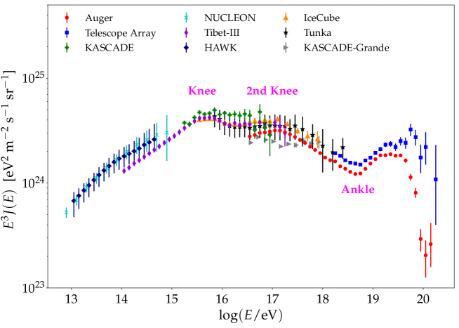
Figure 1: Cosmic-ray flux, multiplied by $E^{3}$, as a function of the logarithmic energy. The data are taken from Refs. AugerJ:19 ; TAJ:19 ; KJ:11 ; NUCJ:19 ; TibetJ:08 ; HawkJ:17 ; IceCubeJ:19 ; TunkaJ:20 ; KGJ:15 . Adapted from Carmeloevoli:21 .

It has long been believed that the galactic cosmic rays dominate the flux at low energies and extragalactic ones at high energies. This is based on the known inefficiencies of the galactic sources to accelerate particles to the highest energies. Moreover, the Pierre Auger Observatory (hereafter Auger) has found strong evidence about the extragalactic origin of the cosmic rays with energies above $10^{18.9}$ eV AugerSc:17 . The transition between the galactic and extragalactic components is still an open problem in cosmic-ray physics. In fact, the scenarios in which the transition takes place at the ankle are disfavored by the Auger data Auger:12 . Therefore, the transition between these two components should take place somewhere between $\sim$$10^{16}$ and $\sim$$10^{18}$ eV.

The determination of the mass composition as a function of the primary energy is crucial to understand many aspects of cosmic rays. However, the main limitation is that the composition determination is based on the comparison of experimental data with EAS simulations. Because the high-energy hadronic interactions relevant for the cosmic rays are unknown, models that extrapolate lower-energy accelerator data are used in shower simulations. This practice introduces systematic uncertainties that can be quite large depending on the shower observable under consideration.

The relevant parameter for the motion of charged particles in magnetic fields is the rigidity, $R=E/(Z\times e)$, where $E$ is the energy of the particle, $Z$ the charge number, and $e$ the absolute value of the electron charge. The trajectories of particles with smaller rigidity values are strongly deviated by a given magnetic field. The acceleration of the cosmic rays and also its propagation on the galactic and extragalactic magnetic field depends on the rigidity. Therefore, the composition information is relevant for the study of the cosmic-ray sources and its propagation through the Galaxy and the intergalactic medium. In fact, due to the intensity of the galactic magnetic field, the identification of extragalactic sources is possible only considering light cosmic rays at the highest energies (large rigidity values) Harari:14 .

The composition information is also very important for the determination of the transition between the galactic and extragalactic components and the origin of the ankle Kampert:12 ; Aloisio:12 . The composition studies are also relevant to constrain the models of the suppression AugerPrime:16 . The composition is also key information to study the high-energy hadronic interactions beyond the reach of man-made accelerators AugerPAir:12 ; TAPAir:20 ; Lipari:20 .

The determination of the composition beyond the ankle is also important to predict the fluxes of cosmogenic photons and neutrinos. These particles are generated as a by-product of the propagation of high-energy nuclei in the intergalactic medium Gaisser:16 . In particular, they are generated due to the interaction of the cosmic rays with the radiation field present in the universe. Higher neutrino and photon fluxes are expected for lighter composition profiles at the highest energies (see, for instance, Ref. Kampert:12 ). Moreover, the measurement of the cosmogenic neutrino and photon fluxes can be very useful to constrain the composition in the suppression region Hooper:11 ; Vliet:19 .

This paper is organized as follows: In Section 2, we discuss the main aspects of the physics of the EAS oriented to composition analyses. In Section 3, we review the composition measurements performed above $10^{15}$ eV by using optical, radio, and surface detectors. In Section 4, we review the photons and neutrinos searches at the highest energies conducted in several experiments. In Section 5, we discuss the future of the composition measurements with current and future detectors. Finally, the main conclusions are discussed in Section 6.

2 Physics of Extensive Air Showers

The characteristics of the EASs initiated by the cosmic rays depend on the primary type. The differences among the EASs initiated by different primary types are used to identify the nature of the primary. Even though the detailed knowledge of the shower characteristics is studied through full Monte Carlo simulations, there are simple models that allow to understand the main physical properties of the EAS. A simple model of electromagnetic showers, i.e., initiated by photons, electrons, or positrons, was first introduced by Heitler Heitler:44 and was extended to hadronic showers by Matthews Matthews:05 .

In the Heitler model, two processes are responsible for the electromagnetic shower development: Bremsstrahlung and pair production undergone by high-energy photons and electrons or positrons, respectively. Each electromagnetic particle (photons, electrons, and positrons) undergoes a two-body splitting at a fixed distance $d=\lambda_{\text{r}}\ln 2$, where $\lambda_{\text{r}}$ is the radiation length in the medium (for the EAS, the medium is the atmosphere). The energy of each mother particle is distributed equally between the two daughter particles. The creation of particles ceases when its energy becomes smaller than the one necessary for undergoing Bremsstrahlung or pair production. Heitler takes this critical energy, $\mathcal{E}_{\text{c}}^{e}$, as the energy for which the radiative energy loss is equal to the collisional energy loss. In this simple model, the maximum of the shower is reached when the energy of each electromagnetic particle is equal to the critical energy. Therefore, $E/2^{n_{\text{c}}}=\mathcal{E}_{\text{c}}^{e}$, where $E$ is the primary energy and $n_{\text{c}}$ is the number of splitting lengths required to reach the maximum. The mean atmospheric depth at which the shower maximum is reached is given by $\langle X_{\textrm{max}}^{\textrm{em}}\rangle=n_{\text{c}}\lambda_{\text{r}}\ln 2$, which, after writing $n_{\text{c}}$ as a function of the primary energy and the critical energy, becomes

$$\langle X_{\textrm{max}}^{\textrm{em}}\rangle=\lambda_{\text{r}}\ln\left(\frac{E}{\mathcal{E}_{\text{c}}^{e}}\right).$$ (1)

This simple model predicts quite well the values of $\langle X_{\textrm{max}}^{\textrm{em}}\rangle$ obtained from simulations. Note that $\langle X_{\textrm{max}}^{\textrm{em}}\rangle$ is linearly dependent on the logarithmic energy.

In the extension of the Heitler model for the hadronic showers developed by Matthews (here on referred to as the Heitler–Matthews model), the atmosphere is also divided by layers of fixed thickness. Both the primary particle and each secondary hadron interact after passing through one layer of the atmosphere. Each hadron produces $N_{\text{ch}}$ charged pions ($\pi^{\pm}$) and $N_{\text{ch}}/2$ neutral pions ($\pi^{0}$). It is assumed that the neutral pions decay into two photons immediately after being created. These high-energy photons initiate electromagnetic showers. The charged pions continue their multiplication process until they all reach the critical energy, $\mathcal{E}_{\text{c}}^{\pi}$, which is taken as the energy for which the pion decay length is equal to the thickness of one layer. At this point, all charged pions decay producing muons and antimuons. Therefore, the hadronic showers are composed of three main components: electromagnetic, muonic, and hadronic (neutrinos and antineutrinos are also created in EASs, mainly in charged pion decays).

Let us consider first showers initiated by protons. Assuming that the energy is equally distributed among all created particles, the number of layers required to reach the point in which all charged pions decay is given by

$$n_{\text{c}}=\frac{\ln\left(E/\mathcal{E}_{\text{c}}^{\pi}\right)}{\ln\left(\frac{3}{2}N_{\text{ch}}\right)},$$ (2)

where $E$ is the energy of the primary proton. As mentioned before, the number of muons (hereafter muons refers to muons and antimuons) is equal to the number of charged pions that reached the critical energy, $N_{\mu}^{p}=N_{ch}^{n_{c}}$. Therefore, using Equation (2), the following expression for the average number of muons is obtained

$$\langle N_{\mu}^{\text{p}}\rangle=\left(\frac{E}{\mathcal{E}_{\text{c}}^{\pi}}\right)^{\beta},$$ (3)

where

$$\beta=\frac{\ln N_{\text{ch}}}{\ln\left(\frac{3}{2}N_{\text{ch}}\right)}.$$ (4)

Therefore, the Heitler–Matthews model predicts a power-law dependence with the primary energy of the muons number in proton-initiated air showers.

In the Heitler–Matthews model, it is assumed that, in the first interaction, one-third of the proton energy is injected into the electromagnetic channel. The neutral pions generated in the subsequent steps of the cascade also feed the electromagnetic channel, but the energy directed to this channel is smaller than the one corresponding to the first interaction. Therefore, in this model, only the first interaction is considered to calculate the mean value of $X_{\textrm{max}}$.

In the first interaction $N_{\text{ch}}/2$, neutral pions are generated. Then, the number of photons generated in the decay of the neutral pions is $N_{\text{ch}}$. The energy of each neutral pion generated in the first interaction is $E_{\pi^{0}\!,\,\text{f}}=E/(3N_{\text{ch}}/2)$, and then the energy of each photon generated after the decays of the neutral pion is $E_{\gamma,\,\text{f}}=E_{\pi^{0}\!,\,\text{f}}/2=E/(3N_{\text{ch}})$. Considering that the mean atmospheric depth of the first interaction is $X_{0}$ and that at this point $N_{\text{ch}}$ showers are initiated by photons of energy $E_{\gamma,\,\text{f}}$, the mean depth of the shower maximum is obtained

$$\langle X_{\textrm{max}}^{\text{p}}\rangle=X_{0}+\lambda_{\text{r}}\ln\left(\frac{E}{3N_{\text{ch}}\,\mathcal{E}_{\text{c}}^{e}}\right).$$ (5)

Equation (5) can be written in terms of the mean value of $X_{\textrm{max}}$ corresponding to photon-initiated showers. By using Equation (1), the following expression is obtained

$$\langle X_{\textrm{max}}^{\text{p}}\rangle=\langle X_{\textrm{max}}^{\gamma}\rangle+X_{0}-\lambda_{\text{r}}\ln\left(3N_{\text{ch}}\right),$$ (6)

where $X_{\textrm{max}}^{\gamma}$ is the atmospheric depth of the maximum shower development of photon-initiated showers.

The elongation rate measures the rate of change of the mean value of $X_{\textrm{max}}$ with logarithmic energy. It is defined as

$$D=\frac{d\langle X_{\textrm{max}}\rangle}{d\ln E}.$$ (7)

Note that if $D_{10}=d\langle X_{\textrm{max}}\rangle/d\log E$, then $D_{10}=\ln(10)D$.

The elongation rate of proton showers can be obtained from Equations (6) and (7). It is given by

$$D_{\text{p}}=D_{\gamma}+\frac{d}{d\ln E}\left(X_{0}-\lambda_{\text{r}}\ln(3N_{\text{ch}})\right),$$ (8)

which implies that $D_{\text{p}}<D_{\gamma}$, because $N_{\text{ch}}$ increases and $X_{0}$ decreases with primary energy. This result is known as the Linsley’s elongation rate theorem Linsley:77 , which states that the elongation rate of showers initiated by any hadron cannot exceed the one corresponding to photon showers.

The number of muons and the depth of the shower maximum for heavier primaries can be obtained from the superposition model. In this simple model, a primary nucleus of mass number $A$ and energy $E$ is considered as $A$ independent nucleus of energy $E/A$ each. This approximation relies on the fact that the binding energy of the nucleus is much smaller than the primary energy (see Ref. Kampert:12 for a more detailed discussion). Therefore, by using the superposition model, the following expressions are obtained

$$\langle N_{\mu}^{A}\rangle=A\,\left(\frac{E}{\mathcal{E}_{\text{c}}^{\pi}A}\right)^{\beta},$$ (9)

$$\langle X_{\textrm{max}}^{A}\rangle=X_{0}+\lambda_{\text{r}}\ln\left(\frac{E}{3N_{\text{ch}}\,\mathcal{E}_{\text{c}}^{e}\,A}\right),$$ (10)

which, from Equations (3) and (5), take the following form

$$\langle N_{\mu}^{A}\rangle=A^{1-\beta}\,\langle N_{\mu}^{\text{p}}\rangle,$$ (11)

$$\langle X_{\textrm{max}}^{A}\rangle=\langle X_{\textrm{max}}^{\text{p}}\rangle-\lambda_{\text{r}}\ln A.$$ (12)

As mentioned before, the detailed study of the EAS characteristics is conducted from full Monte Carlo simulations. The Monte Carlo programs most used in the literature are CORSIKA corsika and AIRES aires . Moreover, the CONEX conex program is widely used in the literature as it combines the Monte Carlo technique with the numerical solution of the cascade equations to obtain the longitudinal development of the showers, which considerably reduces the computing time compared to the full Monte Carlo simulations. The main limitation of the EAS simulations originates from the lack of knowledge of the hadronic interactions at the highest energies. Models that extrapolate the low-energy accelerator data to the required energies are included in the Monte Carlo programs. The high-energy hadronic interaction models commonly used in the literature have been updated recently with the Large Hadron Collider (LHC) data. However, some discrepancies among the predictions obtained from different models are still present, even at LHC energies, due to the limited collider data in the central region, which is relevant for the EAS simulation. These differences in the shower observables predicted by different high-energy hadronic interaction models introduce large systematic uncertainties in composition analyses. The post-LHC high-energy hadronic interaction models most used in the literature are: EPOS-LHC epos , Sibyll 2.3d sibyll , and QGSJet-II.04 qgsjetII .

Despite the strong simplifications in the Heitler–Matthews model, it predicts quite well the functional dependence of the mean number of muons and the mean depth of the shower maximum with primary energy and mass number. However, the mean value of $X_{\textrm{max}}^{A}$ predicted by the model is about 100 g cm^-2 smaller than the one obtained from EAS simulations Matthews:05 . In Ref. Matthews:05 , it is suggested that these discrepancies arise due to the non-inclusion of the photons, originated in neutral pion decays, produced beyond the ones corresponding to the first interaction. In Ref. Montanus:14 , it is found that this is not the origin of the discrepancies. Moreover, in that work, it is proposed that the discrepancies arise from the assumption of a homogeneous distribution of energy among the particles created in each step of the cascade.

As mentioned before, the Heitler–Matthews model predicts the functional dependence of $\langle X_{\textrm{max}}^{A}\rangle$ with $A$ and $E$ (see Equation (12)). This is shown in the analysis performed in Ref. AugerXmax:13 , made based on EAS simulations, where it is found that the mean value of $X_{\textrm{max}}^{A}$ can be written as

$$\langle X_{\textrm{max}}^{A}\rangle=\langle X_{\textrm{max}}^{\text{p}}\rangle+F_{E}\ln A,$$ (13)

where $F_{E}$ is a function of primary energy.

Regarding the number of muons, it is also found that its dependence with $A$ and $E$ can be approximated by the one predicted by the Heitler–Matthews model (see Equation (11)). Moreover, it can be seen that the $\beta$ parameter ranges from $0.85$ to $0.93$ Matthews:05 , such that the values close to $\beta=0.93$ correspond to post-LHC models Cazon:18 .

From the previous discussion, it can be seen that the EAS generated by light nuclei develop deeper in the atmosphere and have a lower muonic content than an EAS generated by heavy nuclei. Therefore, the $X_{\textrm{max}}$ parameter and also any parameter closely related to the muon content of the showers (such as the number of muons at ground, measured at a given distance to the shower axis or even in a given distance range) can be used to determine the nature of the primary particle. Moreover, these two parameters showed to be the best to discriminate between proton and iron primaries (see, for instance, Ref. Supanitsky:08 ).

The longitudinal development of the EAS is characterized by the number of charged particles present at a given slant depth, $N_{\text{ch}}(X)$. However, a quantity that is more closely related to the observation of the longitudinal development of an EAS with fluorescence telescopes is the energy deposition rate $\frac{dE}{dX}$, i.e., the longitudinal profile, whose integral gives the total energy deposited in the atmosphere. Because $N_{\text{ch}}(X)$ is, to a very good approximation, proportional to the longitudinal profile, the maximum reached by both functions is located at approximately the same atmospheric depth.

The left panel of Figure 2 shows the longitudinal profiles of proton and iron showers of $E=10^{19}$ eV, zenith angle $\theta=40^{\circ}$, simulated with CONEX 2r7.5 and EPOS-LHC as the high-energy hadronic interaction model. From the figure, it can be seen that effectively the proton showers develop deeper in the atmosphere than the iron showers. It can also be seen that shower-to-shower fluctuations are larger in the case of proton showers. The right panel of Figure 2 shows the corresponding distributions of $X_{\textrm{max}}$. Note that both the mean value and the standard deviation of $X_{\textrm{max}}$ are both sensitive to the primary mass.

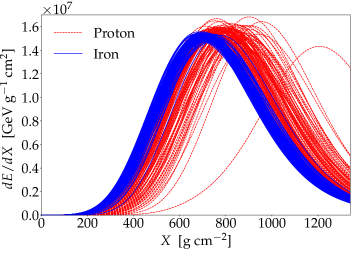
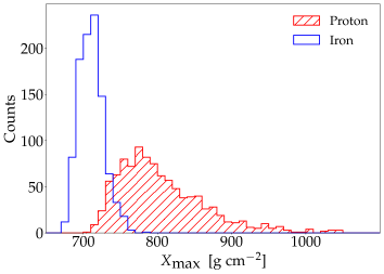
Figure 2: Left: Simulated longitudinal profiles for proton- and iron-initiated air showers. Righ: Depth of the shower maximum distributions for proton- and iron-initiated air showers. The primary energy is $E=10^{19}$ eV and the zenith angle is $\theta=40^{\circ}$. The simulations are performed with EPOS-LHC.

The left panel of Figure 3 shows the number of muons, with energy above 1 GeV, as a function of the atmospheric depth, for proton- and iron-initiated air showers of $E=10^{19}$ eV, $\theta=40^{\circ}$, simulated with CONEX 2r7.5 and EPOS-LHC as the high-energy hadronic interaction model. The right panel of the figure shows the distributions of the total number of muons at ground. They are obtained evaluating $N_{\mu}(X)$ at the atmospheric depth of the observation level, which is located at sea level. From the figure, it can be seen that the iron showers have a larger muon content than proton showers and that the shower-to-shower fluctuations are smaller for iron showers as in the case of $X_{\textrm{max}}$. It can also be seen that the total number of muons is also a very good parameter to discriminate between proton and iron showers. Note that the number of electrons (hereafter electrons will refer to electrons and positrons) of the showers is much larger than the one corresponding to muons. Therefore, the longitudinal development of the muons cannot be observed by using optical detectors.

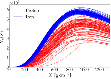
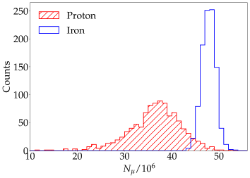
Figure 3: Left: Number of muons as a function of the atmospheric depth for proton- and iron-initiated air showers. Right: Distributions of the total number of muons at ground for proton- and iron-initiated air showers. The primary energy is $E=10^{19}$ eV and the zenith angle is $\theta=40^{\circ}$. The observation level is located at sea level and the threshold energy of the muons is 1 GeV. The simulations are performed with EPOS-LHC.

Figure 4 shows $X_{\textrm{max}}$ as a function of $N_{\mu}$ for proton and iron showers for different values of primary energy. From the figure, it can be seen that these two parameters are very good parameters to separate proton and iron showers from $10^{15}$ to $10^{20}$ eV, i.e., the whole energy range relevant for cosmic-ray detection through EAS observations. It can also be seen that the combination of these two parameters increases the discrimination power with respect to the case in which any of them is considered individually. This is valid for the whole energy range considered.

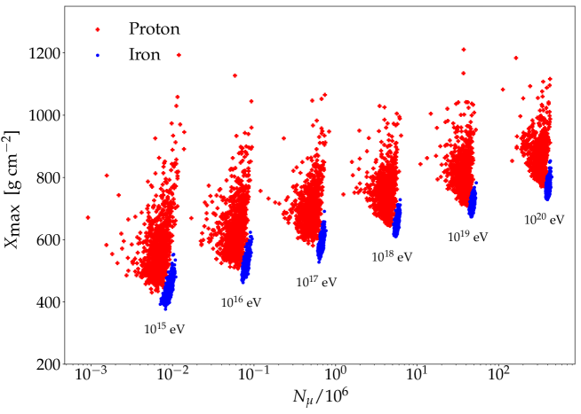
Figure 4: Depth of the shower maximum versus the number of muons at ground level for proton- and iron-initiated air showers and for different values of primary energy. The zenith angle is $\theta=40^{\circ}$. The observation level is located at sea level, the threshold energy of the muons is 1 GeV, and the simulations are performed with EPOS-LHC.

There are many parameters, besides $X_{\textrm{max}}$ and the muon content of the showers, that are sensitive to primary mass. Among others are: the slope of the lateral distribution function, the rise time of the signals collected by ground detectors, the maximum of the muon production depth distribution, etc. Note that all these parameters depend on $X_{\textrm{max}}$ and $N_{\mu}$. In any case, the discrimination power between heavy and light primaries of the $X_{\textrm{max}}$ and $N_{\mu}$ combination increases very little when more mass-sensitive parameters are added Supanitsky:09b .

It is worth mentioning that different cosmic-ray observatories have measured events, different from the vast majority, that cannot be explained with current EAS models AugerTGF:21 ; TATGF:20 ; Beisembaev:21 . These events are characterized by large multiplicities of triggered stations and large signals. Auger and Telescope Array have found that these types of events are observed during thunderstorms. Even though their origin is still unknown, it is believed that those events may originate in bursts of high-energy photons produced during thunderstorms known as downward gamma-ray flashes.

3 Composition Measurements

In general, there are two types of detectors that allow the detection of EASs: the ones that detect the secondary particles of the showers at ground level and the ones that measure the low-energy electromagnetic radiation generated due to the shower front propagation through the atmosphere during the shower development. The secondary particles at ground are measured with surface detectors and the low-energy radiation produced during the shower development is measured with radiation detectors, which include optical and radio detectors.

3.1 Composition from Optical and Radio Detectors

There are two main optical techniques to measure the longitudinal development of the showers, which allow to reconstruct the $X_{\textrm{max}}$ parameter directly. These two experimental techniques involve: fluorescence telescopes and non-imaging Cherenkov detectors. The radio detectors allow to measure the $X_{\textrm{max}}$ parameter in an indirect way.

The fluorescence telescopes measure the fluorescence light emitted by the nitrogen molecules of the atmosphere that are excited by the charged particles of the EAS. The spectrum of the fluorescence light ranges from 300 to 400 ns. The fluorescence light yield is proportional to the energy deposited by the charged particles of the showers in the atmosphere. Therefore, measuring the fluorescence light during the shower development, it is possible to reconstruct the longitudinal profile of the showers. The fluorescence telescopes are composed by a faceted mirror and a camera formed by a large number of small photomultipliers. The telescopes are housed in dedicated climate-controlled buildings. The reconstruction of the longitudinal profile requires the determination of the shower axis. It can be determined observing the shower development with one telescope (monocular observation), but a much better accuracy is achieved when the same shower is observed with two telescopes (stereo observation). A similar accuracy to the one corresponding to the stereo observation is obtained when the data of at least one telescope are combined with the data taken by surface detectors (hybrid observations). Note that the fluorescence telescopes can take data in clear and moonless nights, which reduces the duty cycle to $\sim$$15\%$. Moreover, this experimental technique requires a continuous monitoring of the atmosphere.

The fluorescence technique was used in the past in experiments by the Fly’s Eye flyseye and its successor, HiRes hires . The Fly’s Eye telescope operated 10 years in monocular mode; after that, an additional fluorescence telescope was added in order to perform stereo observations. Therefore, in the second phase of the Fly’s Eye experiment and during the operation of HiRes, it was possible to perform stereo observations. At present, there are two observatories that are currently taking data and make use of this technique: one is Auger Auger and the other one is Telescope Array TA . Both observatories can perform stereo observations as well as hybrid observations.

As mentioned before, the energy deposition rate of the showers, $\frac{dE}{dX}$, can be measured by using the fluorescence technique. The integral of this profile gives the total energy dissipated electromagnetically. Therefore, in the fluorescence technique, the atmosphere is used as a calorimeter and the integral of the longitudinal profile gives the calorimetric energy. The calorimetric energy is $80-90\%$ of the primary energy, and the remaining $10-20\%$ corresponds to the so-called “invisible energy”, which is carried away by neutrinos and high-energy muons and has to be estimated and added to the calorimetric energy in order to reconstruct the primary energy (see Ref. AugerIE:19 for details).

Figure 5 shows the longitudinal profile of a hybrid event detected by Auger AugerFD:10 . The longitudinal profile is fitted with a Gaisser–Hillas function which is given by

$$f_{\text{GH}}(X)=f_{\textrm{max}}\left(\frac{X-X_{0}}{X_{\textrm{max}}-X_{0}}\right)^{\frac{X_{\textrm{max}}-X_{0}}{\lambda}}\exp\left(-\frac{X-X_{\textrm{max}}}{\lambda}\right),$$ (14)

where $f_{\textrm{max}}$, $X_{0}$, $\lambda$, and $X_{\textrm{max}}$ are free-fitting parameters. For the event in the figure, the primary energy is $E_{0}=(3.0\pm 0.2)\times 10^{19}$ eV and the depth of the shower maximum is $X_{\textrm{max}}\cong 723$ g cm^-2.

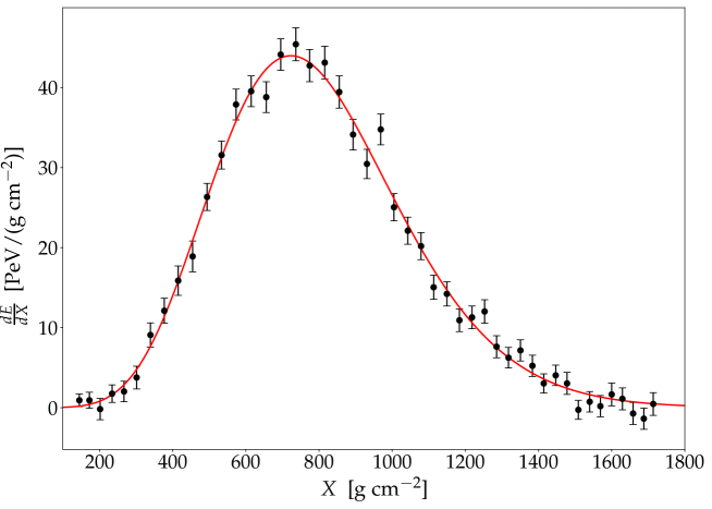
Figure 5: Hybrid event detected by the Pierre Auger Observatory. The solid line corresponds to a fit of the data points with a Gaisser–Hillas function (see Equation (14)). The primary energy of the event is $E=(3.0\pm 0.2)\times 10^{19}$ eV and the maximum is reached at $X_{\textrm{max}}\cong 723$ g cm^-2. Adapted from AugerFD:10 .

It is worth mentioning that the determination of the primary energy by using the fluorescence technique is little influenced by the high-energy hadronic interaction models used to simulate the showers. This is the main reason for the hybrid design of Auger and Telescope Array. In contrast with the fluorescence telescopes, the duty cycle of the surface detectors is $\sim$$100\%$. Therefore, the calibration in energy of the events recorded by the surface detectors only is performed by using hybrid events for which the reconstructed energy is taken as the one obtained from the fluorescence telescopes. In this way, the reconstructed energy of the events recorded by the surface detectors only are subject to smaller systematic uncertainties compared with the case in which the energy calibration is performed by using simulations of the showers.

The non-imaging Cherenkov detectors measured the Cherenkov radiation that is generated by the charged particles of the EAS when they propagate through the atmosphere. Note that the Cherenkov radiation is emitted when a charged particle propagates through a medium at a velocity larger than the speed of light in that medium. The Cherenkov photons are detected by arrays of photomultipliers (like particle detectors) that look upward. The observations are conducted on moonless and clear nights, which reduces the duty cycle to 10–15%. This technique requires a continuous monitoring of the atmosphere. Several cosmic-ray observatories applied the non-imaging Cherenkov technique to detect air showers. The three non-imaging Cherenkov detector arrays that are currently in operation are the ones installed in Yakutsk Ivanov:09 , Tunka Budnev:05 , and in the Telescope Array site called NICHE TANICHE:19 .

The primary energy and the depth of the shower maximum of each detected shower are obtained from the measured lateral distribution function of Cherenkov photons Ivanov:09 ; Dyakonov:86 ; Budnev:05 . The left panel of Figure 6 shows the lateral distribution of Cherenkov photons corresponding to an event measured by the Yakutsk array Knurenko:19 . The primary energy and zenith angle of the event are $E\cong 1.3\times 10^{19}$ eV and $\theta\cong 25^{\circ}$, respectively. The reconstructed depth of the shower maximum is $X_{\textrm{max}}\cong 738$ g cm^-2. Even though the methods to reconstruct the primary energy and $X_{\textrm{max}}$ can be quite sophisticated, it is known that the primary energy is nearly proportional to the photons’ density at 120 m from the shower axis, and the depth of the shower maximum is closely related to the slope of the lateral distribution function Hillas:82 ; Patterson:83 . Note that this technique also allows a calorimetric estimation of the primary energy.

Air showers emit electromagnetic radiation at radio frequencies. This radiation is strongly beamed in the forward direction. The two main mechanisms for the radio emission are geomagnetic and Askaryan emissions Huege:16 ; Schroder:17 . The Cherenkov emission is also present but negligible at radio frequencies. The dominant mechanism is the one associated to the geomagnetic field. In this case, the radiation originates from the interaction of the secondary electrons and positrons of the showers with the geomagnetic field, inducing a time-dependent transverse current. On the other hand, the Askaryan or charge excess emission is produced when the air shower particles ionize the atmosphere, and the ionization electrons are added to the cascade producing a negative charge excess located in the shower front region. Heavy and positive ions remain behind the shower front. In this mechanism, the time-dependent charge excess is responsible for the radio emission.

The radio emission from the EAS is emitted in a wide frequency interval. It has been measured from $\sim$$2$ to $\sim$$500$ MHz. The radio emission is detected through the ground arrays of radio antennas that can measure this radiation in different frequency bands. The radio signal measured by the antennas is not symmetric with respect to the shower axis Huege:16 ; Schroder:17 . These asymmetries depend on the relative contribution of the geomagnetic and charge excess emissions. There are several methods to reconstruct $X_{\textrm{max}}$ from the radio signals Huege:16 ; Schroder:17 . In particular, the slope of the lateral distribution function is used to reconstruct $X_{\textrm{max}}$. The right panel of Figure 6 shows the lateral distribution function of radio, after asymmetry correction, of an event measured by the Tunka experiment TunkaRex:16 .

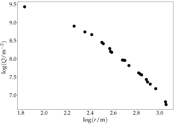
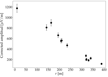
Figure 6: Left: Logarithmic photon density as function of the logarithmic distance to the shower axis (lateral distribution function) of an event measured by the non-imaging Cherenkov detectors of Yakutsk. The primary energy and zenith angle of the event are: $E\cong 1.3\times 10^{19}$ eV and $\theta\cong 25^{\circ}$, respectively. Adapted from Knurenko:19 . Right: Lateral distribution function, after asymmetry correction, of an event measured by the Tunka radio antennas in the 35–76 MHz band. Adapted from TunkaRex:16 .

It is worth mentioning that the radio technique allows a calorimetric determination of the primary energy, and also, the radio antennas have a duty cycle close to $100\%$. The experiments that are operating at present and that have measured $X_{\textrm{max}}$ by using the radio technique are: Auger AugerR:21 , Yakutsk YakutskR:19 , Tunka TunkaR:18 , and LOFAR LofarR:21 .

Figure 7 shows the mean value of the depth of the shower maximum as a function of the logarithmic primary energy measured by different experiments. The figure also shows the predicted values of $\langle X_{\textrm{max}}\rangle$ for proton and iron primaries obtained from shower simulations. The simulated air showers used to obtain the model predictions are generated with CONEX 2r7.5 by using the high-energy hadronic interaction models: Sibyll 2.3d, QJSJet-II.04, and EPOS-LHC. The primary energy of the simulated air showers ranges from $\log(E/\textrm{eV})=15$ to $\log(E/\textrm{eV})=20$ in steps of $\Delta\log(E/\textrm{eV})=1$ and the zenith is $\theta=40^{\circ}$. Finally, the curves in the figure are obtained by fitting the mean value of $X_{\textrm{max}}$ as a function of the logarithmic energy with a second-order polynomial in $\log(E/\textrm{eV})$. Note that the $\langle X_{\textrm{max}}\rangle$ measured by the Telescope Array (TA FD in the figure) is shifted by 5 g cm^-2 to take into account the detector effects Yushkov:18 .

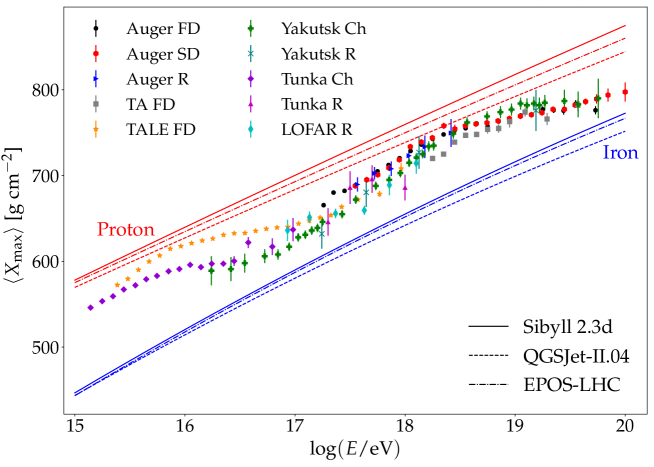
Figure 7: Mean value of $X_{\textrm{max}}$ as a function of the logarithmic energy measured by different experiments. FD, Ch, and R in the legend refer to fluorescence, Chrerenkov, and radio techniques, respectively. The data of Auger are labeled as: Auger FD Yushkov:19 , Auger SD (in this case, $X_{\textrm{max}}$ is obtained from surface detectors data calibrated with the fluorescence detectors data) Peixoto:19 , and Auger R AugerR:21 . The data of Telescope Array are labeled as: TA FD Abbasi:18 and TALE FD Abbasi:21 . The data of Yakutsk are labeled as: Yakutsk Ch Knurenko:19 and Yakutsk R YakutskR:19 . The data of Tunka are labeled as: Tunka Ch Budnev:21 and Tunka R TunkaR:18 . The data of LOFAR are labeled as: LOFAR R LofarR:21 . The curves correspond to model predictions for proton and iron primaries simulated by using different high-energy hadronic interaction models.

From Figure 7, it can be seen that, at low energies, the TALE data present large differences with the Tunka and Yakutsk data. These differences are reduced at energies of the order of and even larger than $10^{17}$ eV. The TALE data are compatible with a light composition at $\sim$$10^{15.4}$ eV that becomes even lighter for increasing energies. At energies close to $10^{16}$ eV, they are compatible with a composition that starts to change, becoming heavier as the energy increases. The Tunka data, starting at $\sim$$10^{15.1}$ eV, are compatible with a light composition that keeps nearly constant up to energies close to $10^{15.8}$ eV. From this point, they are compatible with a composition that becomes heavier for increasing values of the energy. The Yakutsk data, starting at $\sim$$10^{16.24}$ eV, are compatible with the Tunka data in the overlapping energy range. Therefore, even though the experimental data show a transition to heavier primaries from $\sim$$10^{16}$ eV, the differences between experiments suggest the existence of important systematic uncertainties in the experimental techniques used to obtain the mean value of $X_{\textrm{max}}$ as a function of primary energy.

Figure 7 also shows that the Yakutsk data are compatible with a change in the composition profile at $\sim$$10^{17}$ eV. At larger values of the primary energy, these data are compatible with a variable composition that goes from intermediate mass to lighter nuclei. This change is also observed in the TALE and LOFAR data but at higher energies. The Auger data, starting at $10^{17.26}$ eV, are also compatible with a variable composition that becomes lighter for increasing values of primary energy. Between $\sim$$10^{17.5}$ and $\sim$$10^{18.5}$ eV, the data are compatible with a light composition. At $\sim$$10^{18.5}$ eV, these data are compatible with a composition that becomes heavier for increasing values of primary energy. Even though there are differences between the Yakutsk and Auger data, they show a similar trend. Above $\sim$$10^{18.25}$ eV, the Telescope Array data seem to be consistent with a constant and light composition, but it has been shown that it is compatible with Auger data considering current statistical and systematic uncertainties Yushkov:18 .

As mentioned before, the standard deviation of the $X_{\textrm{max}}$ parameter, $\sigma[X_{\textrm{max}}]$, can also be used to study the composition of the primary particle. Not all experiments considered have reported the $\sigma[X_{\textrm{max}}]$ data. Figure 8 shows $\sigma[X_{\textrm{max}}]$ as a function of the logarithmic energy measured by different experiments. The figure also shows the predicted values of $\sigma[X_{\textrm{max}}]$ for proton and iron primaries obtained from shower simulations. The same shower library used to calculate $\langle X_{\textrm{max}}\rangle$ predictions is used to calculate $\sigma[X_{\textrm{max}}]$ predictions. Additionally, in this case, the curves in the figure are obtained by fitting the $\sigma[X_{\textrm{max}}]$ as a function of the logarithmic energy with a second-order polynomial in $\log(E/\textrm{eV})$. Note that $\sigma[X_{\textrm{max}}]$ measured by the Telescope Array (TA FD in the figure) is obtained by subtracting 15 g cm^-2 in the quadrature to take into account the detector effects Batista:19 .

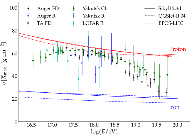
Figure 8: Standard deviation of $X_{\textrm{max}}$ as a function of logarithmic energy measured by different experiments. FD, Ch, and R in the legend refer to fluorescence, Chrerenkov, and radio techniques, respectively. The data of Auger are labeled as: Auger FD Yushkov:19 and Auger R AugerR:21 . The data of Telescope Array are labeled as: TA FD Abbasi:18 . The data of Yakutsk are labeled as: Yakutsk Ch Knurenko:19 and Yakutsk R YakutskR:19 . The data of LOFAR are labeled as: LOFAR R LofarR:21 . The curves correspond to model predictions for proton and iron primaries simulated by using different high-energy hadronic interaction models.

From Figure 8, it can be seen that the lowest energy data reported correspond to Yakutsk. They start at $10^{16.5}$ eV. The Yakutsk data are compatible with a variable composition that seems to be be dominated by intermediate nuclei at the lowest energy and becomes lighter for increasing values of primary energy. The data of the different experiments are compatible with a light composition from $\sim$$10^{17.5}$ to $\sim$$10^{18.5}$ eV, where a transition toward heavier nuclei begins. This picture is compatible with the one inferred considering the mean value of $X_{\textrm{max}}$ in the limited energy range corresponding to $\sigma[X_{\textrm{max}}]$ measurements.

There are several possibilities to study the composition of the cosmic rays from the $X_{\textrm{max}}$ data. From the measured $X_{\textrm{max}}$ distributions, it is possible to infer the abundance of different nuclei that are assumed to be present in the cosmic-ray energy spectrum at a given energy Bellido:18 ; Abbasi:21 . From the measured values of $\langle X_{\textrm{max}}\rangle$, it is possible to infer the mean value of the logarithmic mass number AugerXmax:13 , which is defined as $\langle\ln A\rangle=\sum_{A}f_{A}(E)\ \ln A$, where $f_{A}(E)$ is the fraction of nuclei of mass number $A$ at a given primary energy. Moreover, from the measured values of $\sigma[X_{\textrm{max}}]$, it is possible to estimate the standard deviation of $\ln A$ AugerXmax:13 . All these analyses have to be conducted by using EAS simulations which, as mentioned before, can introduce important systematic uncertainties due to the different predictions obtained when different high-energy hadronic interaction models are considered.

Let us consider the estimation of $\langle\ln A\rangle$ from $\langle X_{\textrm{max}}\rangle$ data. The mean value of $X_{\textrm{max}}$ obtained from measurements involves the average over shower-to-shower fluctuation and also over the mass number, i.e.,

$$\langle X_{\textrm{max}}\rangle=\int_{0}^{\infty}dX_{\textrm{max}}\sum_{A}f_{A}(E)P(X_{\textrm{max}}|A,E)\ X_{\textrm{max}},$$ (15)

where $P(X_{\textrm{max}}|A,E)$ is the distribution function of $X_{\textrm{max}}$ for a given mass number $A$ and primary energy $E$ (see right panel of Figure 2). Equation (15) can also be written as,

$$\langle X_{\textrm{max}}\rangle=\sum_{A}f_{A}(E)\langle X_{\textrm{max}}^{A}\rangle.$$ (16)

Taking the average over $A$ in Equation (13) and using Equation (16), the following expression for $\langle\ln A\rangle$ is obtained

$$\langle\ln A\rangle=\frac{\langle X_{\textrm{max}}\rangle-\langle X_{\textrm{max}}^{\text{p}}\rangle}{\langle X_{\textrm{max}}^{\text{Fe}}\rangle-\langle X_{\textrm{max}}^{\text{p}}\rangle}\ln(56),$$ (17)

where it is used that the function $F_{E}$ in Equation (13) can be written as $F_{E}=(\langle X_{\textrm{max}}^{\text{Fe}}\rangle-\langle X_{\textrm{max}}^{\text{p}}\rangle)/\ln(56)$.

Figure 9 shows $\langle\ln A\rangle$ as a function of the logarithmic energy obtained by using Equation (17). The values of $\langle X_{\textrm{max}}^{\text{Fe}}\rangle$ and $\langle X_{\textrm{max}}^{\text{p}}\rangle$ are obtained from the fits of the simulated EAS data described above. The calculation is performed for the three high-energy hadronic interaction models considered. From the figure, the dependence of the inferred $\langle\ln A\rangle$ on the high-energy hadronic interaction models used to analyze the data is evident. In fact, the lightest composition is found when QGSJet-II.04 is used to analyze the data, and the heaviest composition is found for Sibyll2.3d.

Figure 9 shows more clearly the trend followed by the composition inferred based on Figure 7. For all high-energy hadronic interaction models, a gradual increase in the composition from $\sim$$10^{16}$ eV, reaching a maximum value of $\langle\ln A\rangle$ between $2.6$ and $3$, close to the expectation for nitrogen ($A=14$), can be seen. At some point between $\sim$$10^{17}$ and $\sim$$10^{18}$ eV, a transition toward light nuclei starts. The minimum is reached at $10^{18.3}$–$10^{18.5}$ eV, where a new transition toward heavy elements starts. At energies of the order of $\sim$$10^{20}$ eV, the only available $X_{\textrm{max}}$ data are obtained from the surface detectors of Auger. This is due to the reduced duty cycle of the fluorescence and non-imaging Cherenkov techniques compared with the one corresponding to the surface detectors, which is $\sim$$100\%$. Therefore, at $\sim$$10^{20}$ eV, these data suggest that $\langle\ln A\rangle\cong 2-3$ depending on the high-energy hadronic interaction model considered.

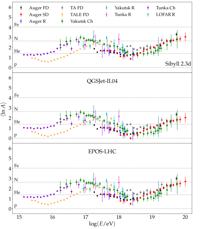
Figure 9: Mean value of $\ln A$ as a function of the logarithmic energy obtained from $\langle X_{\textrm{max}}\rangle$ measured by different experiments. Three different high-energy hadronic interaction models are used to interpret the data.

The change in composition at a break energy of $10^{18.3}$–$10^{18.5}$ eV (the break energy depends on the experimental data considered) has been discussed recently in Refs. Sokolsky:21 ; Watson:22 . In these analyses, it is shown that there is clear experimental evidence about a change in the elongation rate at a given break energy, as first reported by Auger Auger:14 . Moreover, in Ref. Sokolsky:21 , it is claimed that for energies below the break energy, the elongation rate obtained from the data of the northern and southern hemispheres are compatible, but the ones obtained considering data above the break energy are different. In contrast, in the subsequent analysis of Ref. Watson:22 , it is found that the elongation rates measured in the northern and southern hemispheres are compatible below and above the energy break.

3.2 Composition from Surface Detectors

As mentioned before, the composition can also be inferred from data taken by surface detectors that measure the secondary particles of the EAS that reach the ground. These composition analyses are based on a single parameter or on a combination of several parameters. The main advantage of the composition analyses based on surface detectors data is that the duty cycle of these types of detectors is $\sim$$100\%$ and then the number of events is about one order of magnitude larger than the one corresponding to the optical detectors.

In general, it is difficult to compare the results of the analyses based on surface detectors data with the ones obtained from the mean value of the $X_{\textrm{max}}$ parameter due to the fact that $\langle\ln A\rangle$ is not always reported and it is not directly obtained from the data as in the $X_{\textrm{max}}$ parameter case. In this paper, the results of the composition analyses in which $\langle\ln A\rangle$ is reported and the ones corresponding to the measurements of the muon density are considered.

The muon density measured by different experiments cannot be compared directly as it depends on the altitude of the observatory, the threshold energy of the muons, and the single distance to the shower axis or interval of distances to the shower axis considered for its calculation. One way to compare measurements of the muon density from different experiments is through the $z$-scale Dembinski:19 ; Gesualdi:21b . However, in this work, a different approach is followed. Assuming that the muon density, for a primary of mass number $A$, measured by the different experiments, follows Equation (11), i.e., $\langle\rho_{\mu}^{A}\rangle=A^{1-\beta}\langle\rho_{\mu}^{\text{p}}\rangle$, and that the mass number of the heaviest nuclei is $A_{\text{M}}$, the $\langle\ln A\rangle$ can be approximated by Supanitsky:22

$$\langle\ln A\rangle\cong\left(\frac{\langle\rho_{\mu}\rangle}{\langle\rho_{\mu}^{\text{p}}\rangle}-1\right)\frac{\ln A_{\text{M}}}{A_{\text{M}}^{1-\beta}-1}+\frac{\Delta}{2},$$ (18)

where $A_{\text{M}}$ is taken as the minimum mass number such that the data points corresponding to a given muon density-related parameter are contained between the predictions for protons and the one corresponding to nuclei of mass number $A_{\text{M}}$ and

$$\Delta=\left|\frac{A_{\text{M}}^{1-\beta}-1-(1-\beta)\ln A_{\text{M}}}{(A_{\text{M}}^{1-\beta}-1)(1-\beta)}-\frac{1}{1-\beta}\ln\left(\frac{A_{\text{M}}^{1-\beta}-1}{(1-\beta)\ln A_{\text{M}}}\right)\right|.$$ (19)

Here, $\Delta/2$ is the systematic uncertainty introduced by the use of the approximated expression in Equation (18).

Figure 10 shows $\langle\ln A\rangle$ as a function of the logarithmic primary energy obtained by using data from surface detectors. The experiments considered are Auger, IceCube, AGASA, and Telescope Array. In this case, the models considered are EPOS-LHC and QGSJet-II.04. The measurements considered are:

• $\langle\ln A\rangle$ obtained from the $\Delta_{\text{s}}$ parameter, measured by Auger, which is obtained from the risetimes of the signal collected by the water-Cherenkov detectors AugerDeltaS:17 . The data taken by the 750 and 1500 m arrays are considered.

• $\langle\ln A\rangle$ obtained from the parameter $X_{\textrm{max}}^{\mu}$, measured by Auger, which corresponds to the atmospheric depth of the maximum of the muon production depth distribution AugerXmumax:14 . It is obtained from the time traces measured by the water-Cherenkov detectors.

• The parameter $R_{\mu}$, measured by Auger, is an estimator of the total number of muons of energy above $0.3$ GeV, obtained from the data provided by the water-Cherenkov detectors AugerRmu:16 . The events considered correspond to inclined showers and are detected in hybrid mode.

• The muon density at 450 m from the shower axis with a muon threshold energy around $1$ GeV, measured by the Underground Muon Detectors (UMDs) of Auger AugerUMD:20 .

• The density of GeV muons at 600 and 800 m from the shower axis measured by IceCube with the IceTop Array IceCube:22 .

• The density of muons of energy above $0.5$ GeV evaluated at 1000 m from the shower axis measured by AGASA Gesualdi:20 ; Gesualdi:21 .

• $\langle\ln A\rangle$ obtained through a multiparametric analysis based on the Telescope Array surface detectors data TA:21 . Note that the $\langle\ln A\rangle$ is reported for the QGSJet-II.04 and QGSJet-II.03 (and older versions of the QGSJet-II models) but not for EPOS-LHC.

Note that the energy scales used are the ones corresponding to each experiment, but for AGASA, the energy scale from the Spectrum Working Group is used SWG:17 . The only systematic uncertainties included in the plot are the ones introduced by the use of Equation (18) to calculate the $\langle\ln A\rangle$ from the measured muon density.

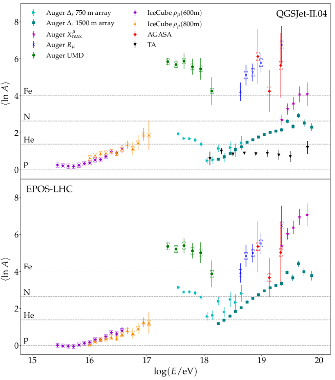
Figure 10: Mean value of $\ln A$ as a function of the logarithmic energy obtained from experimental data taken by the surface detectors of different experiments by using two different high-energy hadronic interaction models to interpret the data. The Auger data are labeled as: Auger $\Delta_{\text{s}}$ 750 m array AugerDeltaS:17 , Auger $\Delta_{\text{s}}$ 1500 m array AugerDeltaS:17 , Auger $X_{\textrm{max}}^{\mu}$ AugerXmumax:14 , Auger $R_{\mu}$ AugerRmu:16 , and Auger UMD AugerUMD:20 . The IceCube data are labeled as: IceCube $\rho_{\mu}$ (600 m) and IceCube $\rho_{\mu}$ (800 m) IceCube:22 . The AGASA data are labeled as: AGASA Gesualdi:20 ; Gesualdi:21 . The Telescope Array data are labeled as: TA TA:21 . The square brackets correspond to the systematic uncertainties introduced by the use of Equation (18) to calculate the $\langle\ln A\rangle$.

From Figure 10, it can be seen that, in general, the $\langle\ln A\rangle$ obtained from surface detectors data is incompatible with the one obtained by optical and radio detectors. Moreover, $\langle\ln A\rangle$ obtained from the Auger UMD and $R_{\mu}$ parameter are compatible with a composition dominated by nuclei heavier than iron, which is incompatible with any realistic astrophysical scenario. This is so for both EPOS-LHC and QGSJet-II.04. The $\langle\ln A\rangle$ obtained from $X_{\textrm{max}}^{\mu}$ is also compatible with a composition dominated by nuclei heavier than iron when EPOS-LHC is considered to analyze the data. When QGSJet-II.04 is considered to interpret the $X_{\textrm{max}}^{\mu}$ data, the $\langle\ln A\rangle$ is compatible with a composition dominated by iron nuclei or even lighter for smaller values of the primary energy. However, the values of $\langle\ln A\rangle$ obtained are incompatible with the ones obtained by using optical and radio detectors. The AGASA data are also compatible with a flux dominated by nuclei heavier than iron. The values of $\langle\ln A\rangle$ obtained by using the $\Delta_{\text{s}}$ parameter are closer to the ones obtained by using optical and radio detectors, but they are still larger than those. The Telescope Array data are compatible with a light composition above $10^{18}$ eV which is also incompatible with the optical and radio results and also with other analyses based on surface detectors data. The IceCube data are also in tension with the optical results, but in this energy range, there are also discrepancies between data obtained by different optical detectors.

The Auger water-Cherenkov detectors measure muons and also the electromagnetic particles of the showers. Close to the shower axis, the signal is dominated by the electromagnetic particles, and far from the shower axis, it is dominated by muons. Therefore, the $\Delta_{\text{s}}$ parameter is less affected by the muon component than the other parameters. Because the $\langle\ln A\rangle$ obtained from the $\Delta_{\text{s}}$ parameter is smaller than the one obtained by using other parameters completely dominated by the muonic component of the showers, the incompatibility seems to originate in the number of muons predicted by the post-LHC high-energy hadronic interaction models. In fact, the much heavier composition inferred from muon density measurements suggests that post-LHC high-energy hadronic interaction models present a deficit in the muon component Albrecht:22 . This muon deficit has been studied in detail by the Working Group on Hadronic Interaction and Shower Physics (WHISP). Combining muon data from several experiments, they find that the muon measurements are compatible with the post-LHC high-energy hadronic interaction models up to energies of a few $10^{16}$ eV. Above that energy, the muon deficit increases with the logarithmic energy (see Ref. WHISP:21 for an updated analysis). The muon deficit can take large values at the highest energies, for instance, Auger found that for $10^{18.8}\,\textrm{eV}\leq E\leq 10^{19.2}\,\textrm{eV}$, it is of the order of $\sim$$33\%$ for EPOS-LHC and $\sim$$61\%$ for QGSJet-II.04 AugerPRL:16 . There is also experimental evidence about the increase in the muon deficit with the zenith angle of the showers AugerPRL:16 ; KASCADEG:18 . It is worth mentioning that the composition inferred from the muon measurements of the Yakutsk EAS array is compatible with the one inferred from the $X_{\textrm{max}}$ measurements Yakutsk:19 . This is so in the whole energy range of the Yakutsk EAS array, which includes the highest energies where the muon deficit found by other experiments is more important. Therefore, further studies of the biases and systematic uncertainties of each experiment are required in order to understand and solve the existing discrepancies.

It is worth mentioning that, despite the tension between the experimental data and the post-LHC high-energy hadronic interaction models, the trends in the change of the mass composition obtained from optical detectors (see Figure 9) are consistent with the ones obtained from surface detectors (see Figure 10).

In order to illustrate the tension between post-LHC high-energy hadronic interaction models and the experimental data, at the level of the composition-sensitive observables, Figure 11 shows the mean values of different parameters measured by using data taken by the UMDs (top panels) and the water-Cherenkov detectors (lower panels) of Auger as a function of the mean value of $X_{\textrm{max}}$ for different values of the primary energy and zenith angle. The curves correspond to the predictions obtained by using EPOS-LHC and QGSJet-II.04. From the figure, it can be seen that the experimental data are incompatible with the predictions of the high-energy hadronic interaction models considered. Note that the experimental points fall outside the curves even when the systematic uncertainties are considered. Moreover, without considering the analysis based on the $X_{\textrm{max}}^{\mu}$ parameter, which is not directly related with the muon content of the showers, it can be seen that the tension between high-energy hadronic interaction models considered and data can be relaxed by increasing the number of muons in the simulated showers.

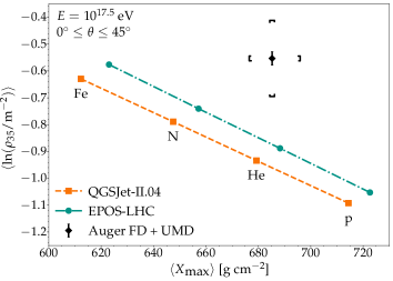
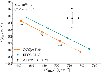
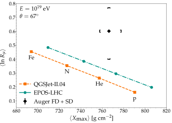
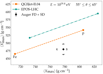
Figure 11: Top panels: Mean value of the logarithmic muon density at 450 m from the shower axis for a reference zenith angle of $35^{\circ}$ as a function of the mean value of $X_{\textrm{max}}$ measured by the Auger UMD. Adapted from AugerUMD:20 . Bottom left panel: Mean value of the natural logarithm of $R_{\mu}$ as a function of the mean value of $X_{\textrm{max}}$ measured by the Auger water-Cherenkov detectors. Adapted from AugerRmu:16 . Bottom right panel: Mean value of $X_{\textrm{max}}^{\mu}$ parameter as a function of the mean value of $X_{\textrm{max}}$ measured by the Auger water-Cherenkov detectors. Adapted from Cazon:19 . The curves correspond to the predictions obtained for EPOS-LHC and QGSJet-II.04.

In the second knee region, KASCADE-Grande could separate the flux in light and heavy components measuring the shower particles with shielded and unshielded surface detectors KG:11 ; KG:13 . Note that with these two types of surface detectors, it is possible to separate the muonic and the electromagnetic components. In this case, the primary energy is reconstructed by using simulated showers. The heavy component presents a knee-like feature at $\sim$$10^{16.7}$–$10^{16.8}$ eV when the data are analyzed with EPOS-LHC, QGSJet-II.04, and Sibyll 2.3d KG:21 . The light component presents a flattening at $\sim$$10^{17}$ eV. At this energy, the flux is dominated by the heavy component. If the cosmic ray flux in the knee region is dominated by protons, the iron knee should take place at $E_{\text{Fe}}^{\text{knee}}=26\times E_{\text{p}}^{\text{knee}}$; therefore, if $E_{\text{p}}^{\text{knee}}=3\times 10^{15}\,\textrm{eV}\cong 10^{15.48}$ eV, then $E_{\text{Fe}}^{\text{knee}}\cong 10^{16.89}$ eV, very close to the knee observed by KASCADE-Grande in the heavy component. In this interpretation, the knee in the heavy component is a signature of the end of the galactic cosmic rays. The ankle-like feature in the light component can be interpreted as the beginning of the transition between galactic and extragalactic cosmic rays KG:13 . In this case, this feature is formed by the superposition of a galactic flux with the extragalactic one which starts to be dominant above $\sim$$10^{17}$ eV.

The increase in the $\langle\ln A\rangle$ measured by TALE above $10^{17}$ eV (see Figure 9) is in tension with this interpretation. Additionally, the iron fraction measured by TALE Abbasi:21 does not show any evidence about the knee in the heavy component observed by KASCADE-Grande. Moreover, the $\langle\ln A\rangle$ measured by IceTop in combination with IceCube also increases above $10^{17}$ eV IceCubeJ:19 . Moreover, in this case, the iron fraction does not show any change below $10^{17}$ eV.

The discrepancies found between data taken by surface detectors in the second knee region can be due to the muon deficit of the simulated showers. As mentioned before, the tension among data taken by optical detectors in this region of the spectrum suggest the existence of large systematic uncertainties. More studies are required to understand the differences found.

3.3 Combined Analyses

The results of a study performed combining data taken by the fluorescence telescopes and the water-Cherenkov detectors of Auger were recently published in Ref. Vicha:21 . The primary energy of the events considered in the analysis ranges from $10^{18.5}$ to $10^{19}$ eV, and the parameters considered are $X_{\textrm{max}}$ and the signal deposited in the water-Cherenkov detectors at 1000 m from the shower axis, $S(1000)$. Assuming that the composition of the cosmic rays is independent of the zenith angle, it was found that to alleviate the tension between the Auger data and EAS simulations, in addition to the increase in the number of muons of the simulated showers, a shift in the simulated $X_{\textrm{max}}$ parameter is also required. If this result is confirmed in future studies, it would imply that the muon deficit alone cannot explain the discrepancies between current high-energy hadronic interaction models and experimental data.

A scaled version of the same parameters has been considered by Auger to study the purity of the cosmic rays in the energy range from $10^{18.5}$ to $10^{19}$ eV. In this case, the correlation between the scaled version of the parameters is used to study the composition Yushkov:19 ; AugerCorr:16 . For energies between $10^{18.5}$ and $10^{18.7}$ eV, a pure composition is excluded with a significance larger than $6.4\,\sigma$. Moreover, the data can be explained only by a mixture of primary nuclei of a mass number heavier than helium, i.e., pure composition, and proton–helium mixtures are disfavored by the data. An important feature of this analysis is that it is nearly independent on the high-energy hadronic interaction models used to analyze the experimental data. Note that this result is consistent with the composition inferred from the $X_{\textrm{max}}$ parameter alone, measured by Auger.

There are two main interpretations about the formation of the ankle and the origin of the light component that dominates the flux between $10^{18}$ and $10^{18.5}$ eV. In the first scenario Aloisio:14 ; Mollerach:20 , the light component below the ankle originates in a different population of sources than the one that dominates the flux above the ankle, which includes heavier nuclei according to the Auger data. In the second scenario, the light component originates from the photodisintegration of high-energy and heavier nuclei in a photon field present in the sources or its environment Unger:15 ; Globus:15a ; Globus:15b ; Kachelriess:17 ; Fang:18 ; Supanitsky:18 . In these two scenarios, the transition between the galactic and extragalactic components takes place in the second knee region.

4 High-Energy Photon and Neutrino Searches

Ultra-high-energy photons and neutrinos carry very important information about the cosmic-ray accelerators and the propagation of the cosmic rays in the intergalactic medium. In particular, its arrival direction points back to the source, as they are neutral particles and then they are not deflected by the galactic and extragalactic magnetic fields. Moreover, knowing the photon flux level is very important for an accurate energy calibration of surface detectors with fluorescence telescopes (see, for instance, Ref. AugerPRL:08 ).

As mentioned before, a flux of high-energy photons and neutrinos is expected due to the interaction of the extragalactic cosmic rays with the radiation field present in the intergalactic medium. Nuclei of ultra-high energies can interact with the low-energy photons of the extragalactic background light, the cosmic microwave background, and the radio background. Neutrinos are produced in pion decays, generated through photo-pion production and nuclear decay. The main decay channels of charged pions are: $\pi^{+}\rightarrow\mu^{+}+\nu_{\mu}\rightarrow e^{+}+\nu_{e}+\bar{\nu}_{\mu}+\nu_{\mu}$ and $\pi^{-}\rightarrow\mu^{-}+\bar{\nu}_{\mu}\rightarrow e^{-}+\bar{\nu}_{e}+\nu_{\mu}+\bar{\nu}_{\mu}$. Note that the muon decay also contributes to the neutrino generation. The expected flavor ratio at Earth is $1:1:1$ due to neutrino oscillations. Photons are produced in neutral pion decays ($\pi^{0}\rightarrow\gamma+\gamma$), generated in photo-pion production, and also due to the inverse Compton of high-energy electrons with low-energy photons of the background ($e^{\pm}+\gamma_{b}\rightarrow e^{\pm}+\gamma$). Note that high-energy electrons are generated by the pair production of high-energy nuclei with the low-energy photons of the background. They are also created in the beta decay of nuclei and the decay of muons from the decay of charged pions. The high-energy photons and electrons form an electromagnetic cascade in the intergalactic medium.

High-energy photons arriving at Earth generate EASs that are almost electromagnetic. They are characterized by having a much deeper $X_{\max}$ and very small muon content. For this reason, it is easier to separate hadrons from photons than heavy from light hadrons. At present, there are only upper limits to the integrated photon flux obtained by different experiments. The most restrictive ones are obtained by Auger and Telescope Array, which are shown in Figure 12. The figure also shows the integrated photon flux corresponding to two extreme models in which the ultra-high-energy cosmic-ray flux is dominated by protons and by iron nuclei Kampert:12 . From the figure, it can be seen that the upper limits are reaching the integrated flux values corresponding to the proton model.

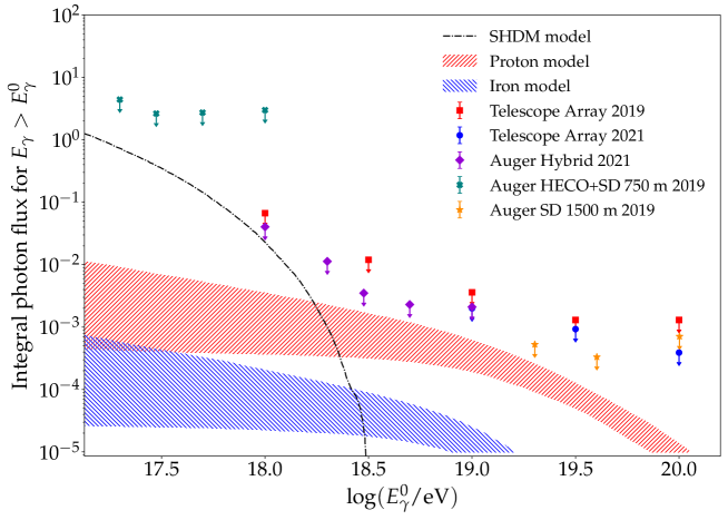
Figure 12: Upper limits on the integral photon flux at $95\%$ confidence level obtained by Auger AugerPh:19 ; AugerPh:21 and Telescope Array TAPh:19 ; TAPh:21 . The shaded regions correspond two models in which the ultra-high-energy cosmic rays are dominated by protons and iron nuclei Kampert:12 . The dashed-dotted curve corresponds to the integral photon flux originated by the decay of hypothetical super-heavy dark matter particles of mass $M_{\chi}=10^{10}$ GeV/c² and lifetime $\tau_{\chi}=3\times 10^{23}$ year Kalashev:16 . Adapted from AugerPh:21 .

Photon searches at the highest energies have been motivated in the past by the top-down models, in which the ultra-high-energy cosmic rays originate in the decay of super-heavy relic particles present in the halo of our Galaxy or by the decay of topological defects (see Ref. Batacharjee:00 ). In these models, the ultra-high-energy cosmic-ray flux is dominated by photons. These top-down models are disfavored by current data, but it is still possible that a minority component contributes to the total flux. Figure 12 shows the high-energy integral photon flux due to the decay of super-heavy dark matter particles, located in the halo of our Galaxy, of mass $M_{\chi}=10^{10}$ GeV/c² (c is the speed of light) and lifetime $\tau_{\chi}=3\times 10^{23}$ year Kalashev:16 . From the figure, it can be seen that such a model is still compatible with the most stringent upper limits found up to now.

The neutrino search at the highest energies is conducted by using different experimental techniques. There are two main methods to search for neutrinos in cosmic-ray observatories. The first is based on the fact that the neutrino cross section is so small that it is more probable that a neutrino initiates a shower close to the horizontal direction and very deep in the atmosphere. One of these showers is very easy to identify, as hadronic or even electromagnetic showers develop significantly earlier in the atmosphere. The other method is based on the fact that tau neutrinos that propagate skimming the Earth, of zenith angles larger than 90^∘, can interact in the Earth and produce a tau lepton, which can decay in the atmosphere, initiating a shower. These showers are also easy to identify because they develop in the up-going direction.

There are also dedicated neutrino observatories, such as IceCube, which is a cubic-kilometer particle detector made of Antarctic ice. It is buried beneath the surface, reaching a depth of about 2.5 km. In this case, neutrinos are detected when they interact with the molecules of the ice, producing relativistic charged particles, which emit Cherenkov radiation measured with optical modules. These optical modules are placed in a hexagonal grid of 85 strings starting at 1450 m and reaching 2450 m depth. On the other hand, ANITA consists of an array of radio antennas installed on a balloon flying at a height of $\sim$$37$ km in Antarctica. ANITA was designed to measure impulsive radio emissions from a neutrinos-initiated cascade in the Antarctic ice. It can also observe extensive air showers induced by cosmic rays or other particles.

Figure 13 shows the upper limits on the differential neutrino flux, at a $90\%$ confidence level, obtained by IceCube IceCubeUL:18 , Auger AugerNuUL:10 , and ANITA ANITA:19 , which are the most restrictive. In the figure, the expected neutrino flux for the same models considered before can also be seen. Note that the IceCube and Auger upper limits are reaching the flux level of the proton models.

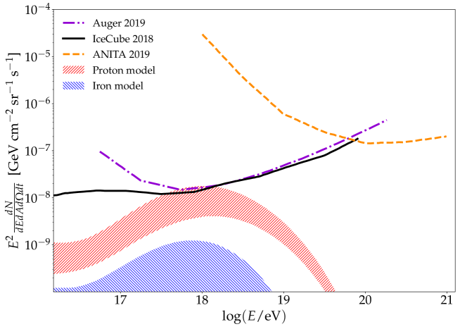
Figure 13: Upper limits on the differential total neutrino flux at $90\%$ confidence level obtained by IceCube IceCubeUL:18 , Auger AugerNuUL:10 , and ANITA ANITA:19 . The shaded regions correspond to two models (same as the ones in Figure 12) in which the ultra-high-energy cosmic rays are dominated by protons and iron nuclei Kampert:12 .

As mentioned in the introduction, the composition at the highest energies is a crucial information for predicting the ultra-high-energy photon and neutrino fluxes. Another important parameter is the maximum energies reached by the cosmic rays injected by the sources. The models that best fit the Auger flux and composition predict very low neutrino and photon fluxes Batista:191 . However, the neutrino flux predicted by the models that best fit the Telescope Array flux and composition is larger TAFit:21 . This is mainly due to the larger values of the fitted maximum energy and also, but to a lesser extent, to the fitted lighter composition. In any case, more statistics in the suppression region are required to obtain a more accurate fit of the data.

Additionally, the ultra-high-energy photons and neutrinos fluxes can constrain the composition of the ultra-high-energy cosmic rays independently of the high-energy hadronic interaction models Hooper:11 ; Vliet:19 . As can be seen from Figures 12 and 13, the neutrino and photon fluxes in models dominated by light nuclei are larger than the ones dominated by heavy nuclei. This is mainly due to the fact that the threshold energy of the photo-pion production increases with the mass number and, because the injection spectrum decreases with the cosmic ray energy, there are less particles in heavy nuclei dominated models that undergo photo-pion production.

5 Future Perspectives on Composition

The data considered in previous sections were taken by detectors that are currently in operation. These experiments will continue taking data and refining the methods used in composition analyses. An example of the progress in the methods used to study the composition is the increasing use of machine learning techniques IceCubeJ:19 ; TA:21 ; AugerDL:21 ; AugerRNN:21 , which have proven to be powerful tools for reconstructing composition sensitive parameters and also in the composition determination.

Some of the current observatories will be or are being upgraded. In particular, Auger started an upgrade of the observatory, which has the detailed study of the composition from the transition region up to the highest energies as one of its main objectives. The Auger upgrade is known as AugerPrime AugerPrime:16 ; AugerPrime:18 . The improvements relevant for composition are: the addition of plastic scintillation detectors on top of the water-Cherenkov detectors to separate the electromagnetic from the muonic components of the showers; the addition of underground muon detectors in the infill region to measure the muonic component of the showers in the transition region; the extension of the current fluorescence telescopes measurements into periods of higher night-sky background in order to increase their duty cycle; and the addition of a radio detector to each water-Cherenkov station which can measure $X_{\textrm{max}}$ and other composition-sensitive parameters. These enhancements will increase the mass composition sensitivity of the observatory. One of the main goals of the upgrade is to measure the composition at the highest energies, in the suppression region, by using the upgraded surface detectors, which can collect about one order of magnitude more statistics than the fluorescence detectors.

Additionally, Telescope Array started an upgrade of the observatory called TAx4 TAx4:21 . It consists of an increase in the detection area by adding new surface detectors and fluorescence telescopes. The detection area increased from $\sim$$700$ to $\sim$$2800$ km². With this new detection area, it will be possible to measure the composition from the northern hemisphere by using both surface and fluorescence detectors with much larger statistics.

IceCube is also planning an upgrade called the IceCube-Upgrade IceCubeUp:21 . It will consist of an enhancement of the IceTop surface detectors by adding scintillation detectors, radio detectors, and possibly small non-image Cherenkov telescopes. One of the main goals of this upgrade is also to increase the mass composition sensitivity of the observatory.

Next generation observatories are currently being planned. In particular, IceCube-Gen2 IceCubeGen2 , the successor of IceCube, will measure cosmic rays at low energies. It will consist of an optical array in the deep ice, a large-scale radio array, and a surface detector above the optical array. It will be able to measure composition with more sensitivity and it will increase its maximum energy up to $\sim$$10^{18}$ eV. At the highest energies, the POEMMA project is designed to measure ultra-high-energy cosmic rays and neutrinos from the space POEMMA:21 . It will consist of two identical orbital fluorescence telescopes being able to measure the $X_{\textrm{max}}$ parameter at the highest energies with unprecedented statistics. The GRAND project GRAND:21 is designed to detect ultra-high-energy neutrinos, cosmic rays, and gamma rays by using the radio technique. It will consist of $2\times 10^{5}$ radio antennas covering an area of $2\times 10^{5}$ km², which will be separated into 20 sub-arrays of $\sim$$10^{4}$ km². It will be able to measure the $X_{\textrm{max}}$ parameter in a wide energy range with large statistics. Finally, GCOS is a starting project intended to design a next-generation observatory with an aperture of at least one order of magnitude larger than the one corresponding to the observatories that are currently in operation GCOS:21 . One of its main objectives is to improve the mass resolution, based on the experience obtained from AugerPrime and TAx4.

The data collected by the planned upgrades and also by the future observatories will constrain even more the high-energy hadronic models used in shower simulations. Moreover, analyses like the one reported in Ref. AugerMuFluct:21 , where the fluctuations of the $R_{\mu}$ parameter are studied and compared with model predictions, can contribute to understand more deeply the discrepancies found. Moreover, the data from the high-luminosity LHC HLLHC:20 run will play an important role on the improvement of the current high-energy hadronic interaction models.

6 Conclusions

The origin of cosmic rays is still an open issue in high-energy astrophysics. The composition of the primary particle is key information to understanding this phenomenon. In the last years, a big effort has been made to determine it. The main limitation comes from the incompatibility of current high-energy hadronic interaction models, used to simulate the EAS required to determine the primary mass, with the experimental data.

The determination of the composition is mainly achieved by using optical detectors that measure the depth of the shower maximum. In particular, the mean value of $X_{\textrm{max}}$ measured by different experiments falls between the proton and iron expectations obtained by using current high-energy hadronic interaction models. There are also several composition parameters that come from the surface detector of which the most sensitive to the nature of the primary is the muon content of the showers. In general, the composition obtained from parameters measured by surface detectors is incompatible with the one obtained from $X_{\textrm{max}}$. These discrepancies are larger at the highest energies, where the composition obtained by some of the parameters falls above the expectations for iron nuclei, obtained by using current models. These incompatibilities are usually interpreted as a deficit in the number of muons predicted by current high-energy hadronic interaction models. Even though the hadronic part of the simulated cascades seems to be the source of the discrepancies, the electromagnetic part, which affects the $X_{\textrm{max}}$ predictions, can also play an important role as showed by recent analyses.

In the energy interval between $10^{15}$ and $10^{18}$ eV, the composition obtained from the $\langle X_{\textrm{max}}\rangle$ measured by different experiments presents large differences. The composition measurement in this energy range is very important for understanding the nature of the second knee, which can be interpreted as the region where the transition between the galactic and extragalactic component takes place, as suggested by the KASCADE-Grande data. The IceCube data cannot corroborate this hypothesis, but this can be due to the systematic uncertainties introduced by current high-energy hadronic interaction models used to analyze the experimental data, which were showed to be more important in composition analyses based on surface detectors information.

Above $\sim$$10^{18}$ eV, the composition measurements obtained by different experiments that measured the $\langle X_{\textrm{max}}\rangle$ are compatible within statistical and systematic uncertainties. The composition seems to be light between $10^{18}$ and $10^{18.5}$ eV. At higher energies, the composition is compatible with an increasingly heavier average mass as a function of primary energy. In this energy region, the discrepancies between the composition obtained from the $X_{\textrm{max}}$ parameter and the muon component of the showers are the largest.

The importance of the composition information on many aspects of cosmic ray studies has become more relevant in recent years. This motivated several upgrades of current observatories with a special interest in the increase in the mass sensitivity of the detectors. Moreover, the next generation of cosmic-ray observatories are also being designed, taking into account the importance of the mass composition determination. Moreover, the planned, much larger detection areas in combination with the enhanced mass composition sensitivity of future detectors will allow to constrain or even measure the photon and neutrino fluxes at the highest energies, which can be used to constrain the composition in the suppression region.

An improvement on current high-energy hadronic interaction models is required to make progress on the composition determination. This can be achieved in the near future, based on the synergy between the EAS studies and the ones conducted in particle physics, especially with the future high-luminosity LHC data.

This research was supported by CONICET, PIP 11220200102979CO.

Not applicable.

Not applicable.

- (1) Verzi, V.; [Pierre Auger Collaboration]. Measurement of the energy spectrum of ultra-high energy cosmic rays using the Pierre Auger Observatory. In Proceedings of the 36th International Cosmic Ray Conference, Madison, WI, USA, 24 July–1 August 2019; p. 450.
- (2) Matthews, J.N.; Telescope Array Collaboration. Highlights from the Telescope Array. In Proceedings of the 35th International Cosmic Ray Conference (ICRC2017), Busan, Korea, 12–20 July 2017; p. 1096.
- (3) Finger, M. Reconstruction of Energy Spectra for Different Mass Groups of High-Energy Cosmic Rays. Ph.D. Thesis, Karlsruhe Institute of Technology, Karlsruhe, Germany, 2011.
- (4) Gorbunov, N.; Grebenyuk, V.; Karmanov, D.; Kovalev, I.; Kudryashov, I.; Kurganov, A.; Panov, A.; Podorozhny, D.; Porokhovoy, S.; Sveshnikova, L.; et al. Energy spectra of abundant cosmic-ray nuclei in the NUCLEON experiment. Adv. Space Res. 2019, 64, 2546–2558.
- (5) Amenomori, M.; Bi, X.J.; Chen, D.; Cui, S.W.; Danzengluobu; Ding, L.K.; Ding, X.H.; Fan, C.; Feng, C.F.; Feng, Z.Y.; et al. [The Tibet AS Collaboration]. The All-Particle Spectrum of Primary Cosmic Rays in the Wide Energy Range from to eV Observed with the Tibet-III Air-Shower Array. Astrophys. J. 2008, 678, 1165–1179.
- (6) Alfaro, R.; et al. [HAWC Collaboration]. All-particle cosmic ray energy spectrum measured by the HAWC experiment from 10 to 500 TeV. Phys. Rev. D 2017, 96, 122001.
- (7) Aartsen, M.G.; et al. [IceCube Collaboration]. Cosmic ray spectrum and composition from PeV to EeV using 3 years of data from IceTop and IceCube. Phys. Rev. D 2019, 100, 082002.
- (8) Budnev, N.M.; Chiavassa, A.; Gress, O.A.; Gress, T.I.; Dyachok, A.N.; Karpov, N.I.; Kalmykov, N.N.; Korosteleva, E.E.; Kozhin, V.A.; Kuzmichev, L.A.; et al. The primary cosmic-ray energy spectrum measured with the Tunka-133 array. Astropart. Phys. 2020, 117, 102406.
- (9) Bertaina, M.; et al. [KASCADE-Grande Collaboration]. KASCADE-Grande energy spectrum of cosmic rays interpreted with post-LHC hadronic interaction models. In Proceedings of the 34th International Cosmic Ray Conference (PoS ICRC2015), The Hague, The Netherlands, 30 July–6 August 2015; p. 359.
- (10) Carmelo, E. The Cosmic Ray Spectrum. 2021. Available online: https://github.com/carmeloevoli/The_CR_Spectrum (accessed on 29 May 2022).
- (11) Aab, A.; et al. [Pierre Auger Collaboration]. Observation of a Large-scale Anisotropy in the Arrival Directions of Cosmic Rays above eV. Science 2017, 357, 1266–1270.
- (12) Abreu, P.; Aglietta, M.; Ahlers, M.; Ahn, E.J.; Albuquerque, I.F.M.; Allard, D.; Allekotte, I.; Allen, J.; Allison, P.; Almela, A.; et al. Large-scale distribution of arrival directions of cosmic rays detected above eV at the Pierre Auger Observatory. Astrophys. J. Suppl. Ser. 2012, 203, 34.
- (13) Harari, D. Ultra-high energy cosmic rays. Phys. Dark Univ. 2014, 4, 23–30.
- (14) Kampert, K.H.; Unger, M. Measurements of the cosmic ray composition with air shower experiments. Astropart. Phys. 2012, 35, 660–678.
- (15) Aloisio, R.; Berezinsky, V.; Gazizov, A. Transition from galactic to extragalactic cosmic rays. Astropart. Phys. 2012, 39–40, 129–143.
- (16) Aab, A.; et al. [Pierre Auger Collaboration]. The Pierre Auger Observatory Upgrade—Preliminary Design Report. arXiv 2016, arXiv:1604.03637.
- (17) Abreu, P.; et al. [Pierre Auger Collaboration]. Measurement of the Proton-Air Cross Section at TeV with the Pierre Auger Observatory. Phys. Rev. Lett. 2012, 109, 062002.
- (18) Abbasi, R.U.; et al. [Telescope Array Collaboration]. Measurement of the proton-air cross section with Telescope Array’s Black Rock Mesa and Long Ridge fluorescence detectors, and surface array in hybrid mode. Phys. Rev. D 2020, 102, 062004.
- (19) Lipari, P. Spectra and composition of ultrahigh-energy cosmic rays and the measurement of the proton-air cross section. Phys. Rev. D 2020, 103, 103009.
- (20) Gaisser, T.K.; Engel, R.; Resconi, E. Cosmic Rays and Particle Physics, 2nd ed.; Cambridge University Press: Cambridge, UK, 2016.
- (21) Hooper, D.; Taylor, A.; Sarkar, S. Cosmogenic photons as a test of ultra-high energy cosmic ray composition. Astropart. Phys. 2011, 34, 340–343.
- (22) van Vliet, A.; Batista, R.A.; Hörandel, J.R. Determining the fraction of cosmic-ray protons at ultrahigh energies with cosmogenic neutrinos. Phys. Rev. D 2019, 100, 021302.
- (23) Heitler, W. The Quantum Theory of Radiation, 3rd ed.; Oxford University Press: London, UK, 1954; p. 386.
- (24) Matthews, J. A Heitler model of extensive air showers. Astropart. Phys. 2005, 22, 387–397.
- (25) Linsley, J. Structure of Large Air Showers at Depth 834 g cm-2 Applications. In Proceedings of the International Cosmic Ray Conference (15th ICRC) Plovdiv, Bulgaria, 13–26 August 1977; Volume 12, pp. 89–96.
- (26) Heck, D.; Knapp, J.; Capdevielle, J.N.; Schatz, G.; Thouw, T. CORSIKA: A Monte Carlo Code to Simulate Extensive Air Showers; Tech. Rep. FZKA-6019; Forschungszentrum Karlsruhe: Germany, 1998.
- (27) Sciutto, S.J. AIRES: A System for Air Shower Simulations. Available online: http://aires.fisica.unlp.edu.ar (accessed on 30 May 2022).
- (28) Bergmann, T.; Engel, R.; Heck, D.; Kalmykov, N.N.; Ostapchenko, S.; Pierog, T.; Thouw, T.; Werner, K. One-dimensional hybrid approach to extensive air shower simulation. Astropart. Phys. 2007, 26, 420–432.
- (29) Pierog, T.; Karpenko, I.; Katzy, J.M.; Yatsenko, E.; Werner, K. EPOS LHC: Test of collective hadronization with data measured at the CERN Large Hadron Collider. Phys. Rev. C 2015, 92, 034906.
- (30) Riehn, F.; Engel, R.; Fedynitch, A.; Gaisser, T.; Stanev, T. Hadronic interaction model SIBYLL 2.3d and extensive air showers. Phys. Rev. D 2020, 102, 063002.
- (31) Ostapchenko, S. Monte Carlo treatment of hadronic interactions in enhanced Pomeron scheme: I QGSJET-II model. Phys. Rev. D 2011, 83, 014018.
- (32) Montanus, J.M.C. An extended Heitler-Matthews model for the full hadronic cascade in cosmic air showers. Astropart. Phys. 2014, 59, 4–11.
- (33) Abreu, P.; Aglietta, M.; Ahlers, M.; Ahn, E.J.; Albuquerque, I.F.M.; Allekotte1, I.; Allen, J.; Allison, P.; Almela, A.; Alvarez Castillo, J.; et al. Interpretation of the depths of maximum of extensive air showers measured by the Pierre Auger Observatory. J. Cosmol. Astropart. Phys. 2013, 02, 026.
- (34) Cazon, L.; Conceição, R.; Riehn, F. Probing the energy spectrum of hadrons in proton air interactions at ultrahigh energies through the fluctuations of the muon content of extensive air showers. Phys. Lett. B 2018, 784, 68–76.
- (35) Supanitsky, A.D.; Etchegoyen, A.; Medina-Tanco, G.; Allekotte, I.; Berisso, M.G.; Medina, M.C. Underground muon counters as a tool for composition analyses. Astropart. Phys. 2008, 29, 461–470.
- (36) Supanitsky, A.D.; Etchegoyen, A.; Medina-Tanco, G. On the possibility of primary identification of individual cosmic ray showers. Astropart. Phys. 2009, 31, 116–127.
- (37) Colalillo, R.; et al. [Pierre Auger Collaboration]. Downward Terrestrial Gamma-ray Flashes at the Pierre Auger Observatory? In Proceedings of the 37th International. Cosmic Ray Conference (PoS ICRC2021), Berlin, Germany, 12–23 July 2021; p. 395.
- (38) Belz, J.W.; et al. [Telescope Array Collaboration]. Observations of the Origin of Downward Terrestrial Gamma-Ray Flashes. J. Geophys. Res. Atmos. 2020, 125, e2019JD031940.
- (39) Beisembaev, R.; Beznosko, D.; Beisembaeva, E.; Dalkarov, O.D.; Mossunov, V.; Ryabov, V.; Shaulov, S.; Vildanova, M.; Zhukov, V.; Baigarin, K.; et al. Spatial and Temporal Characteristics of EAS with Delayed Particles. In Proceedings of the (PoS ICRC2021), 2021; p. 195.
- (40) Baltrusaitis, R.M.; Cady, R.; Cassiday, G.L.; Cooper, R.; Elbert, J.W.; Gerhardy, P.R.; Ko, S.; Loh, E.C.; Salamon, M.; Steck, D.; et al. The Utah Fly’s Eye detector. Nucl. Instrum. Methods Phys. Res. Sect. A 1985, 240, 410–428.
- (41) Abu-Zayyad, T.; Al-Seady, M.; Belov, K.; Chen, G.; Dai, H.Y.; Huang, M.A.; Jui, C.C.H.; Kieda, D.B.; Loh, E.C.; Matthews, J.N.; et al. The prototype high-resolution Fly’s Eye cosmic ray detector. Nucl. Instrum. Methods Phys. Res. Sect. A 2000, 450, 253–269.
- (42) Aab, A.; et al. [Pierre Auger Collaboration]. The Pierre Auger Cosmic Ray Observatory. Nucl. Instrum. Methods Phys. Res. A 2015, 798, 172–213.
- (43) Fukushima, M. Telescope Array Project for Extremely High Energy Cosmic Rays. Prog. Theor. Phys. Suppl. 2003 151, 206–210.
- (44) Aab, A.; et al. [Pierre Auger Collaboration]. Data-driven estimation of the invisible energy of cosmic ray showers with the Pierre Auger Observatory. Phys. Rev. D 2019, 100, 082003.
- (45) Abraham, J.; et al. [Pierre Auger Collaboration]. The fluorescence detector of the Pierre Auger Observatory. Nucl. Instrum. Meth. A 2010, 620, 227–251.
- (46) Ivanov, A.; Knurenko, S.; Sleptsov, I. Measuring extensive air showers with Cherenkov light detectors of the Yakutsk array: the energy spectrum of cosmic rays. New J. Phys. 2009, 11, 065008.
- (47) Budnev, N.M.; Chernov, D.V.; Gress, O.A.; Gress, T.I.; Korosteleva, E.E.; Kuzmichev, L.A.; Lubsandorzhiev, B.K.; Pankov, L.V.; Parfenov, Y.V.; Prosin, V.V.; et al. Cosmic Ray Energy Spectrum and Mass Composition from 1015 eV to 1017 eV by Data of the Tunka EAS Cherenkov Array. In Proceedings of the 29th International Cosmic Ray Conference, Pune, India, 3–11 August 2005; Volume 6, pp. 257–260.
- (48) Omura, Y.; et al. [Telescope Array Collaboration]. Energy spectrum and the shower maxima of cosmic rays above the knee region measured with the NICHE detectors at the TA site. In Proceedings of the 37th International Cosmic Ray Conference, Berlin, Germany, 12–23 July 2021; p. 329.
- (49) Dyakonov, M.N.; Knurenko, S.P.; Kolosov, V.A.; Krasilnikov, D.D.; Lischenyuk, F.F.; Sleptsov, I.E. The use of Cherenkov detectors at the Yakutsk cosmic ray air shower array. Nucl. Instrum. Meth. A 1986, 248, 224–226.
- (50) Knurenko, S.; Petrov, S.; Mass composition of cosmic rays above 0.1 EeV by the Yakutsk array data. Adv. Space Res. 2019, 64, 2570–2577.
- (51) Hillas, A. The sensitivity of Cherenkov radiation pulses to the longitudinal development of cosmic ray showers. J. Phys. G Nucl. Phys. 1982, 8, 1475–1492.
- (52) Patterson, J.; Hillas, A. The relation of the lateral distribution of Cerenkov light from cosmic-ray showers to the distance of maximum development. J. Phys. G Nucl. Phys. 1983, 9, 1433–1452.
- (53) Huege, T. Radio detection of cosmic ray air showers in the digital era. Phys. Rep. 2016, 620, 1–52.
- (54) Schröder, F. Radio detection of cosmic-ray air showers and high-energy neutrinos. Prog. Part. Nucl. Phys. 2017, 93, 1–68.
- (55) Bezyazeekov, P.A.; et al. [Tunka-Rex Collaboration]. Radio measurements of the energy and the depth of the shower maximum of cosmic-ray air showers by Tunka-Rex. J. Cosmol. Astropart. Phys. 2016, 01, 052.
- (56) Pont, B.; et al. [Pierre Auger Collaboration]. The depth of the shower maximum of air showers measured with AERA. In Proceedings of the 37th International Cosmic Ray Conference, Berlin, Germany, 12–23 July 2021; p. 387.
- (57) Petrov, I.; Knurenko, S.; Petrov, Z. Ultra-High Energy Cosmic Ray Study Results by Radio Emission Technique at Yakutsk Array. Phys. At. Nucl. 2019, 82, 795–799.
- (58) Bezyazeekov, P.A.; et al. [Tunka-Rex Collaboration]. Reconstruction of cosmic ray air showers with Tunka-Rex data using template fitting of radio pulses. Phys. Rev. D 2018, 97, 122004.
- (59) Corstanje, A.; Buitink, S.; Falcke, H.; Hare, B.M.; Hörandel, J.R.; Huege, T.; Krampah, G.K.; Mitra, P.; Mulrey, K.; Nelles, A.; et al. Depth of shower maximum and mass composition of cosmic rays from 50 PeV to 2 EeV measured with the LOFAR radio telescope. Phys. Rev. D 2021, 103, 102006.
- (60) Yushkov, A.; et al. [Pierre Auger and Telescope Array Collaborations]. Depth of maximum of air-shower profiles: testing the compatibility of measurements performed at the Pierre Auger Observatory and the Telescope Array experiment. EPJ Web Conf. 2019, 210, p. 01009.
- (61) Yushkov, A.; et al. [Pierre Auger Collaboration]. Mass composition of cosmic rays with energies above 1017.2 eV from the hybrid data of the Pierre Auger Observatory. In Proceedings of the 36th International Cosmic Ray Conference, Madison, WI, USA, 24 July–1 August 2019; p. 482.
- (62) Peixoto, C.; et al. [Pierre Auger Collaboration]. Estimating the Depth of Shower Maximum using the Surface Detectors of the Pierre Auger Observatory. In Proceedings of the 36th International Cosmic Ray Conference, Madison, WI, USA, 24 July–1 August 2019; p. 440.
- (63) Abbasi, R.; et al. [Telescope Array Collaboration]. Depth of Ultra High Energy Cosmic Ray Induced Air Shower Maxima Measured by the Telescope Array Black Rock and Long Ridge FADC Fluorescence Detectors and Surface Array in Hybrid Mode. Astrphys. J. 2018, 858, 76.
- (64) Abbasi, R.; et al. [Telescope Array Collaboration]. The Cosmic-Ray Composition between 2 PeV and 2 EeV Observed with the TALE Detector in Monocular Mode. Astrphys. J. 2021, 909, 178.
- (65) Budnev, N.; et al. [TAIGA Collaboration]. TAIGA—An advanced hybrid detector complex for astroparticle physics, cosmic ray physics and gamma-ray astronomy. In Proceedings of the 37th International Cosmic Ray Conference, Berlin, Germany, 12–23 July 2021; p. 731.
- (66) Batista, R.A.; Biteau, J.; Bustamante, M.; Dolag, K.; Engel, R.; Fang, K.; Kampert, K.; Kostunin, D.; Mostafa, M.; Murase, K.; et al. Open Questions in Cosmic-Ray Research at Ultrahigh Energies. Front. Astron. Space Sci. 2019, 6, 23.
- (67) Bellido, J.; et al. [Pierre Auger Collaboration]. Depth of maximum of air-shower profiles at the Pierre Auger Observatory: Measurements above eV and Composition Implications. n Proceedings of the 35th International Cosmic Ray Conference, Bexco, Busan, Korea, 10–20 July, 2017; p. 506.
- (68) Sokolsky, P.; D’Avignon, R. The Unreasonable Effectiveness of the Air-Fluorescence Technique in Determining the EAS Shower Maximum. arXiv 2021, arXiv:2110.09588.
- (69) Watson, A. Further evidence for an increase of the mean mass of the highest-energy cosmic-rays with energy. J. High Energy Phys. 2022, 33, 14–19.
- (70) Aab, A.; et al. [Pierre Auger Collaboration]. Depth of maximum of air-shower profiles at the Pierre Auger Observatory. I. Measurements at energies above eV. Phys. Rev. D 2014, 90, 122005.
- (71) Dembinski, H.P.; Arteaga-Velázquez, J. C.; Cazon, L.; Conceição, R.; Gonzalez, J.; Itow, Y.; Ivanov, D.; Kalmykov, N. N.; Karpikov, I.; Müller, S.; et al. Report on Tests and Measurements of Hadronic Interaction Properties with Air Showers. In Proceedings of the EPJ Web Conf. 2019, 210, p. 02004.
- (72) Gesualdi, F.; Dembinski, H.; Shinozaki, K.; Supanitsky, D.; Pierog, T.; Cazon, L.; Soldin, D.; Conceição, R. On the muon scale of air showers and its application to the AGASA data. In Proceedings of the 37th International Cosmic Ray Conference, Berlin, Germany, 12–23 July 2021; p. 473.
- (73) Supanitsky, A.D. ITeDA (CNEA-CONICET-UNSAM), San Martin, Prov. de Buenos Aires, Argentina. 2022, manuscript in preparation.
- (74) Aab, A.; et al. [Pierre Auger Collaboration]. Inferences on mass composition and tests of hadronic interactions from 0.3 to 100 EeV using the water-Cherenkov detectors of the Pierre Auger Observatory. Phys. Rev. D 2017, 96, 122003.
- (75) Aab, A.; et al. [Pierre Auger Collaboration]. Muons in air showers at the Pierre Auger Observatory: Measurement of atmospheric production depth. Phys. Rev. D 2014, 90, 012012.
- (76) Aab, A.; et al. [Pierre Auger Collaboration]. Muons in air showers at the Pierre Auger Observatory: Mean number in highly inclined events. Phys. Rev. D 2015, 91, 032003.
- (77) Aab, A.; et al. [Pierre Auger Collaboration]. Direct measurement of the muonic content of extensive air showers between and eV at the Pierre Auger Observatory. Eur. Phys. J. C 2020, 80, 751.
- (78) Abbasi, R.; et al. [IceCube Collaboration]. Density of GeV muons in air showers measured with IceTop. arXiv 2022, arXiv:2201.12635.
- (79) Gesualdi, F.; Supanitsky, A.D.; Etchegoyen, A. Muon deficit in air shower simulations estimated from AGASA muon measurements. Phys. Rev. D 2020, 101, 083025.
- (80) Gesualdi, F.; Supanitsky, A.D.; Etchegoyen, A. Muon deficit in simulations of air showers inferred from AGASA data. In Proceedings of the 37th International Cosmic Ray Conference, Berlin, Germany, 12–23 July 2021; p. 326.
- (81) Zhezher, Y.; et al. [Telescope Array Collaboration]. Cosmic-ray mass composition with the TA SD 12-year data. In Proceedings of the 37th International Cosmic Ray Conference, Berlin, Germany, 12–23 July 2021; p. 300.
- (82) Ivanov, D.; et al. [Pierre Auger and the Telescope Array Collaborations]. Report of the Telescope Array–Pierre Auger Observatory working group on energy spectrum. In Proceedings of the 35th International Cosmic Ray Conference, Bexco, Busan, Korea, 10–20 July, 2017; p. 498.
- (83) Albrecht, J.; Cazon, L.; Dembinski, H.; Fedynitch, A.; Kampert, K.; Pierog, T.; Rhode, W.; Soldin, D.; Spaan, B.; Ulrich, R.; et al. The Muon Puzzle in cosmic-ray induced air showers and its connection to the Large Hadron Collider. Astrophys. Space Sci. 2022, 367, 27.
- (84) Soldin, D.; et al. [EAS-MSU, IceCube, KASCADE-Grande, NEVOD-DECOR, Pierre Auger, SUGAR, Telescope Array, and Yakutsk EAS Array Collaborations]. Update on the Combined Analysis of Muon Measurements from Nine Air Shower Experiments. In Proceedings of the 37th International Cosmic Ray Conference, Berlin, Germany, 12–23 July 2021; p. 349
- (85) Aab, A.; et al. [Pierre Auger Collaboration]. Testing Hadronic Interactions at Ultrahigh Energies with Air Showers Measured by the Pierre Auger Observatory. Phys. Rev. Lett. 2016, 192001.
- (86) Apel, W.D.; et al. [KASCADE-Grande Collaboration]. Probing the evolution of the EAS muon content in the atmosphere with KASCADE-Grande. Astropart. Phys. 2017, 95, 25–43.
- (87) Glushkov, A.V.; Saburov, A.V. Mass Composition of Cosmic Rays with Energies above eV According to the Data from the Muon Detectors of the Yakutsk EAS Array. JETP Lett. 2019, 109, 559–563.
- (88) Cazon, L. Probing High-Energy Hadronic Interactions with Extensive Air Showers. In Proceedings of the 36th International Cosmic Ray Conference, Madison, WI, USA, 24 July–1 August 2019; p. 005.
- (89) Apel, W.D.; et al. [KASCADE-Grande Collaboration]. Kneelike Structure in the Spectrum of the Heavy Component of Cosmic Rays Observed with KASCADE-Grande. Phys. Rev. Lett. 2011, 107, 171104.
- (90) Apel, W.D.; et al. [KASCADE-Grande Collaboration]. Ankle-like feature in the energy spectrum of light elements of cosmic rays observed with KASCADE-Grande. Phys. Rev. D 2013, 87, 081101.
- (91) Kang, D.; et al. [KASCADE-Grande Collaboration]. Results from the KASCADE-Grande Data Analysis. In Proceedings of the 37th International Cosmic Ray Conference, Berlin, Germany, 12–23 July 2021; p. 313.
- (92) Vícha, J.; et al. [Pierre Auger Collaboration]. Adjustments to Model Predictions of Depth of Shower Maximum and Signals at Ground Level using Hybrid Events of the Pierre Auger Observatory. In Proceedings of the 37th International Cosmic Ray Conference, Berlin, Germany, 12–23 July 2021; p. 310.
- (93) Aab, A.; et al. [Pierre Auger Collaboration]. Evidence for a mixed mass composition at the ‘ankle’ in the cosmic-ray spectrum. Phys. Lett. B 2016, 762, 288–295.
- (94) Aloisio, R.; Berezinsky, V.; Blasi, P. Ultra high energy cosmic rays: Implications of Auger data for source spectra and chemical composition. J. Cosmol. Astropart. Phys. 2014, 10, 020.
- (95) Mollerach, S.; Roulet, E. Extragalactic cosmic rays diffusing from two populations of sources. Phys. Rev. D 2020, 101, 103024.
- (96) Unger, M.; Farrar, G.R.; Anchordoqui, L.A. Origin of the ankle in the ultrahigh energy cosmic ray spectrum, and of the extragalactic protons below it. Phys. Rev. D 2015, 92, 123001.
- (97) Globus, N.; Allard, D.; Mochkovitch, R.; Parizot, E. UHECR acceleration at GRB internal shocks. Mon. Not. R. Astron. Soc. 2015, 451, 751–790.
- (98) Globus, N.; Allard, D.; Parizot, E. A complete model of the cosmic ray spectrum and composition across the Galactic to extragalactic transition. Phys. Rev. D 2015, 92, 021302.
- (99) Kachelrieß, M.; Kalashev, O.; Ostapchenko, S.; Semikoz, D.V. Minimal model for extragalactic cosmic rays and neutrinos. Phys. Rev. D 2017, 96, 083006.
- (100) Fang, K.; Murase, K. Linking high-energy cosmic particles by black-hole jets embedded in large-scale structures. Nat. Phys. 2018, 14, 396–398.
- (101) Supanitsky, A.D.; Cobos, A.; Etchegoyen, A. Origin of the light cosmic ray component below the ankle. Phys. Rev. D 2018, 98, 103016.
- (102) Abraham, J.; et al. [Pierre Auger Collaboration]. Observation of the Suppression of the Flux of Cosmic Rays above eV. Phys. Rev. Lett. 2008, 101, 061101.
- (103) Rautenberg, J.; et al. [Pierre Auger Collaboration]. Limits on ultra-high energy photons with the Pierre Auger Observatory. In Proceedings of the 36th International Cosmic Ray Conference, Madison, WI, USA, 24 July–1 August 2019; p. 398.
- (104) Savina, P.; et al. [Pierre Auger Collaboration]. A search for ultra-high-energy photons at the Pierre Auger Observatory exploiting air-shower Universality. In Proceedings of the 37th International Cosmic Ray Conference, Berlin, Germany, 12–23 July 2021; p. 373.
- (105) Abbasi, R.U.; et al. [Telescope Array Collaboration]. Constraints on the diffuse photon flux with energies above eV using the surface detector of the Telescope Array experiment. Astropart. Phys. 2019, 110, 8–14.
- (106) Kalashev, O.E.; et al. [Telescope Array Collaboration]. Telescope Array search for EeV photons. In Proceedings of the 37th International Cosmic Ray Conference, Berlin, Germany, 12–23 July 2021; p. 864.
- (107) Kalashev, O.E.; Kuznetsov, M.Y. Constraining heavy decaying dark matter with the high energy gamma-ray limits. Phys. Rev. D 2016, 94, 063535.
- (108) Bhattacharjee, P.; Sigl, G. Origin and propagation of extremely high-energy cosmic rays. Phys. Rep. 2000, 327, 109–247.
- (109) Aartsen, M.G.; et al. [IceCube Collaboration]. Differential limit on the extremely-high-energy cosmic neutrino flux in the presence of astrophysical background from nine years of IceCube data. Phys. Rev. D 2018, 98, 062003.
- (110) Aab, A.; et al. [Pierre Auger Collaboration]. Probing the origin of ultra-high-energy cosmic rays with neutrinos in the EeV energy range using the Pierre Auger Observatory. J. Cosmol. Astropart. Phys. 2019, 10, 022.
- (111) Gorham, P.W.; et al. [ANITA Collaboration]. Constraints on the ultrahigh-energy cosmic neutrino flux from the fourth flight of ANITA. Phys. Rev. D 2019, 99, 122001.
- (112) Batista, R.A.; de Almeida, R.M.; Lago, B.; Kotera, K. Cosmogenic photon and neutrino fluxes in the Auger era. J. Cosmol. Astropart. Phys. 2019, 01, 002.
- (113) Bergman, D.R.; et al. [Telescope Array Collaboration]. Telescope Array Combined Fit to Cosmic Ray Spectrum and Composition. In Proceedings of the 37th International Cosmic Ray Conference, Berlin, Germany, 12–23 July 2021; p. 338.
- (114) Aab, A.; et al. [Pierre Auger Collaboration]. Deep-learning based reconstruction of the shower maximum using the water-Cherenkov detectors of the Pierre Auger Observatory. J. Instrum. 2021, 16, P07019.
- (115) Aab, A.; et al. [Pierre Auger Collaboration]. Extraction of the muon signals recorded with the surface detector of the Pierre Auger Observatory using recurrent neural networks. J. Instrum. 2021, 16, P07016.
- (116) Castellina, A.; et al. [Pierre Auger Collaboration]. AugerPrime: The Pierre Auger Observatory Upgrade. In Proceedings of the EPJ Web Conf. 2019, 210, 06002.
- (117) Kido, E.; et al. [Telescope Array Collaboration]. Current status and prospects of surface detector of the TAx4 experiment. In Proceedings of the 37th International Cosmic Ray Conference, Berlin, Germany, 12–23 July 2021; p. 203.
- (118) Abbasi, R.; et al. [IceCube Collaboration]. Cosmic-Ray Studies with the Surface Instrumentation of IceCube. In Proceedings of the 37th International Cosmic Ray Conference, Berlin, Germany, 12–23 July 2021; p. 336.
- (119) Aartsen, M.G.; et al. [IceCube-Gen2 Collaboration]. IceCube-Gen2: The Window to the Extreme Universe. J. Phys. G 2021, 48, 060501.
- (120) Olinto, A.V.; et al. [POEMMA collaboration]. The POEMMA (Probe of Extreme Multi-Messenger Astrophysics) observatory. J. Cosmol. Astropart. Phys. 2021, 06, 007.
- (121) Kotera, K.; et al. [GRAND Collaboration]. The Giant Radio Array for Neutrino Detection (GRAND) Project. In Proceedings of the 37th International Cosmic Ray Conference, Berlin, Germany, 12–23 July 2021; p. 1181.
- (122) Hörandel, J.R.; et al. [GCOS Collaboration]. GCOS—The Global Cosmic Ray Observatory. In Proceedings of the 37th International Cosmic Ray Conference, Berlin, Germany, 12–23 July 2021; p. 027.
- (123) Aab, A.; et al. [Pierre Auger Collaboration]. Measurement of the Fluctuations in the Number of Muons in Extensive Air Showers with the Pierre Auger Observatory. Phys. Rev. Lett. 2021, 126, 152002.
- (124) Béjar Alonso, I.; Brüning, O.; Fessia, P.; Rossi, L.; Tavian, L.; Zerlauth, M. High-Luminosity Large Hadron Collider (HL-LHC): Technical design report V.1.0; Number CERN-2020-010, in CERN Yellow Reports: Monographs; CERN: Geneva, Switzerland, 2020.