The spin Hall effect

Abstract

In metallic systems with spin-orbit coupling a longitudinal charge current may generate a transverse pure spin current; vice-versa an injected pure spin current may result in a transverse charge current. Such direct and inverse spin Hall effects share the same microscopic origin: intrinsic band/device structure properties, external factors such as impurities, or a combination of both. They allow all-electrical manipulation of the electronic spin degrees of freedom,i.e. without magnetic elements, and their transverse nature makes them potentially dissipationless. It is customary to talk of spin Hall effects in plural form, referring to a group of related phenomena typical of spin-orbit coupled systems of lowered symmetry.

Key points/objectives

• History and definition of the effect(s)

• Phenomenology and concepts: spin-orbit coupling in solids, charge vs. spin currents, bulk vs. edge effects

• Experiments: from low- to room temperature, diversity and complexity of setups

• Theory: the challenge of complexity, competition between different microscopic mechanisms, Onsager reciprocity

• The broader context: generalisations of the spin Hall effect(s) and suggested further readings

I Introduction

A charge-carrying state in a metallic system is a (non-equilibrium) momentum-ordered state of an electronic ensemble: a collection of quasielectrons moving preferentially in a given direction, see Fig. 1 (a). However quasielectrons carry around their internal spin degrees of freedom, too. For their ensemble to be spin carrying some form of spin order is needed. There are two basic scenarios:

• Spin order is independent of momentum order. This is the situation in a ferromagnet, where the spins of charge carriers align with the magnetisation via exchange coupling independently of their orbital motion.

• Spin and momentum orders are correlated. This is possible in the presence of spin-orbit coupling, which quite generally creates correlations between orbital motion (momentum) and spin.

Consider the second scenario, and to be definite the somewhat special situation sketched in Fig. 1 (b), where quasiparticles with opposite spin projection along $z$ move in opposite directions. An ensemble of such particles does not carry any overall charge – the associated charge current is zero, ${\bf j}^{c}=0$ – but it does carry angular momentum: it is a pure spin-carrying state sustaining a “pure spin current” ${\bf j}^{s}\neq 0$

$${\bf j}^{c} \equiv q\left({\bf j}^{\uparrow}+{\bf j}^{\downarrow}\right)=0$$ (1)

$${\bf j}^{s} \equiv \frac{\hbar}{2}\left({\bf j}^{\uparrow}-{\bf j}^{\downarrow}\right)\neq 0,$$ (2)

with $q$ the quasiparticle charge and $\hbar$ the reduced Planck constant.

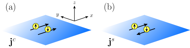
Figure 1: Left panel: A charge current ${\bf j}^{c}$ along $x$, i.e. an overall spin-unpolarised ensemble of quasielectrons moving in the $y$ direction. Right panel: A $z$-polarised pure spin current ${\bf j}^{s}$ flowing along $x$.

In the presence of spin-orbit coupling a transverse ${\bf j}^{s}$ can be generated from a longitudinal ${\bf j}^{c}$, or vice-versa, see Fig. 2. These are respectively the spin Hall effect (sHe)[1, 2] and its reciprocal version, the inverse spin Hall effect (isHe)[3, 4]. The sHe was first predicted by Dyakonov and Perel in 1971 [1] but got his current name only in 1999, when Hirsch [2] sort of re-discovered it and its fortune really started. The isHe followed a similar path. In the geometry from Fig. 2 one has

$$j^{s}_{y} = (\hbar/q)\theta^{\rm sHe}j^{c}_{x},$$ (3)

$$j^{c}_{x} = (q/\hbar)\theta^{\rm isHe}j^{s}_{y}$$ (4)

with $\theta^{\rm sHe},\theta^{\rm isHe}$ the spin Hall and inverse spin Hall angles. Note that from now on upper (lower) indices will denote charge/spin (real space) components. The spin Hall/inverse spin Hall angles are crucial quantities used as standard measure for the spin-charge conversion efficiency of a given setup [5, 6, 7, 8]. In Secs. II and IV we will show that their existence can be expected based on crude but general arguments, while their precise origin and values are extremely sensitive to the microscopic details of the system.

The sHe and isHe exist also in quantised form. Indeed, the “quantum spin Hall insulator” is the paradigmatic example of a time-reversal symmetric two-dimensional topologically insulating phase [9]. The latter is a phase of matter which is insulating in the bulk but hosts two perfectly conducting edge states which are time-reversed partners – up electrons moving in one direction, down in the opposite. In simple terms, a quantum spin Hall phase can be thought of as two time-reversed copies of a (time-reversal broken) quantum Hall state. Its existence was confirmed experimentally in HgCdTe quantum wells in 2007 [10]. I will not discuss it further here, but refer the interested reader to the Encyclopedia Chapter “Topological Effects”.

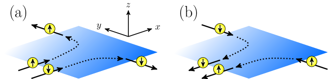
Figure 2: Left panel: spin Hall effect. An $x$-flowing charge current is injected, and a $z$-polarised pure spin current along $y$ is generated via spin-orbit coupling. Right panel: inverse spin Hall effect, where the role of the spin and charge currents are exchanged. Note that in the sHe/isHe the charge current, spin current and the spin quantisation axis are all orthogonal to each other.

The sHe and isHe are nowadays routinely employed in metallic systems to inject and/or read out spin signals via electrical means, and their technological relevance is rapidly on the rise since the early 2000s [3, 4, 8, 11]. The rest of the Chapter will focus uniquely on them. In particular I will not discuss the anomalous Hall effects, closely related phenomena which require however to break time-reversal symmetry [3, 12]. The reader should indeed keep in mind that the spin Hall effect I will deal with in this Chapter actually belongs to a larger class of phenomena which may appear whenever quasiparticles with internal structure move in a non-trivial medium, i.e. not just in the vacuum.

II Phenomenology and basic concepts

II.1 The role of spin-orbit coupling

Take an electron moving with velocity ${\bf v}$ in presence of an electric field ${\bf E}$. In its reference frame the electron sees a velocity-dependent magnetic field

$${\bf B}^{\prime}({\bf v})=-\gamma\frac{{\bf v}}{c}\times{\bf E},\quad\gamma=\frac{1}{\sqrt{1-v^{2}/c^{2}}}$$ (5)

which couples to its spin ${\bf s}=(\hbar/2)\mbox{\boldmath$\sigma$}$, with $\sigma$ the vector of Pauli matrices, as usual

$$H_{\rm so}\sim{\bf s}\cdot{\bf B}^{\prime}\sim{\bf s}\cdot\left({\bf v}\times{\bf E}\right).$$ (6)

Here $c$ is the speed of light. This is a primitive derivation of the spin-orbit interaction.

Let us assume that ${\bf E}=-\nabla V_{\rm ext}$ comes from an external source, e.g. the (random) electrostatic potential from an impurity, see Fig. 3 (a). The quasiparticle spin thus couples to a non-homogeneous field $B^{\prime}({\bf v},{\bf r})$, similarly to what happens in a Stern-Gerlach apparatus. This has various consequences, e.g. it causes spin-flip (Elliot-Yafet) relaxation, but in particular it results in a spin-dependent force ${\bf F}\sim-\nabla\left[{\bf s}\cdot{\bf B}^{\prime}\right]$ orthogonal to ${\bf v}$

$$F_{\perp}^{\uparrow}=-F_{\perp}^{\downarrow}\sim-\nabla_{\perp}B^{\prime}.$$ (7)

This sideway separation of spin-up and spin-down quasiparticles is referred to as Mott skew scattering, and can split an incoming flux of unpolarised electrons into a transverse pure spin current, i.e. it yields a finite $\theta^{\rm sHe}$. It is an “extrinsic” mechanism requiring the presence of scattering centres [3, 2, 4, 13], but a finite $\theta^{\rm sHe}$ may also have origins which are “intrinsic” to the device and/or band structure. Consider for example ${\bf E}=-\nabla V_{\rm int}(z)$, with $V_{\rm int}(z)$ an internal potential which defines your structure, see Fig. 3 (b). Such a potential breaks $z$ inversion symmetry and constrains electrons to move in the $x$-$y$ plane, as in semiconductor quantum wells. One has

$$H_{\rm so}\sim{\bf s}\cdot\left({\bf v}\times e_{z}\right).$$ (8)

Now ${\bf s}$ couples to a homogeneous ${\bf B}^{\prime}({\bf v})$ which always points in plane, called a Rashba field [14, 15]. The eigenstates of the problem are spinors whose quantisation axis depends on their direction of motion. As sketched in Fig. 3 (b), under an electrical bias one expects spin-momentum correlations to arise leading to a transverse, out-of-plane-polarised spin current – that is, to a non-vanishing $\theta^{\rm sHe}$. Recall that in this intrinsic example inversion symmetry was explicitly broken. Some form of spatial symmetry-breaking is indeed a requirement of intrinsic scenarios beyond the present Rashba case [4, 15]. On the other hand time-reversal symmetry is preserved by spin-orbit interaction.

Besides the canonical intrinsic and extrinsic mechanisms just described, other sources for the spin Hall effects include dynamical couplings with phonons [16, 17] or spin fluctuations [18], the interplay of impurity and magnon scattering [19], or fluctuations of the Rashba field [20]. Irrespectively of the origin, and just as a normal Hall current, the spin Hall current is transverse with respect to the drift velocity and thus potentially dissipationless.

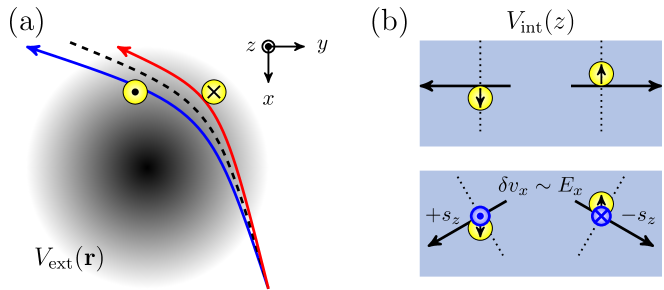
Figure 3: Left panel: Electrons with opposite spins are deflected differently by a scattering potential $V_{\rm ext}({\bf r})$. The dashed black line is the trajectory without spin-orbit corrections. Right panel: Electrons confined to two dimensions by $V_{\rm int}(z)$. The internal velocity-dependent field, see Eq. (8), defines the spin quantisation axis, shown with dotted lines. The two electrons are time-reversed partners, and when driven by an electric field along $x$ their spins will precess around the new (tilted) quantisation axis, yielding out-of-plane components $\pm s_{z}$ shown in blue. The result is a $z$-polarised spin current in the transverse $y$ direction.

II.2 Size and form of (effective) spin-orbit coupling

Since charge carriers in a metallic system move at the Fermi velocity $v_{F}\ll c$, should one expect $H_{\rm so}$ to be only a negligible relativistic correction? The answer is “not necessarily”. Electrons in solids do not move in the vacuum, but constantly get close to ionic cores from the lattice where unscreened very strong electric fields exist, compensating for their (relativistically) slow velocity. One can indeed show that $s$-wave Bloch electrons close to the Fermi energy feel an effective spin-orbit interaction which reads

$$H_{\rm so}=\lambda\mbox{\boldmath$\sigma$}\times\nabla\delta V\cdot{\bf p},$$ (9)

with $\delta V$ any potential other than that of the host lattice, e.g. $\delta V=V_{\rm ext}$ or $\delta V=V_{\rm int}(z)$ from our previous examples. While the form of $H_{\rm so}$ is the same as in the vacuum, the coupling constant $\lambda$ is an effective Compton wavelength strongly renormalised by the lattice: $\lambda/\lambda_{0}\sim 10^{6}$, with $\lambda_{0}$ the vacuum Compton wavelength. The standard machinery behind such renormalization is ${\bf k}\cdot{\bf p}$ theory, which, together with some auxiliary techniques (Löwding partitioning, Schrieffer-Wolff transformation,…), is just a systematic way of building low-energy models starting from the band structure (Bloch states) of a given lattice – at the simplest level it leads e.g. to the effective mass description of electrons in solids [15, 4]. Eq. (9) can actually be generalised to

$$H_{\rm so}={\bf b}({\bf p})\cdot\mbox{\boldmath$\sigma$},$$ (10)

which looks like Zeeman coupling with a momentum-dependent internal field ${\bf b}({\bf p})$. The latter defines a momentum space spin texture – its vectorial image in reciprocal space – of central importance well beyond spin Hall physics. This form of effective spin-orbit interaction is valid beyond the two example scenarios previously introduced, and is the starting point for most discussions of spin-orbit coupled transport phenomena [4, 15].

II.3 A closer look at spin currents

The spin Hall/inverse spin Hall angles, see Eqs. (3), (4), are crucial quantities in spin Hall physics. However to define them one needs to know exactly what a spin current is, which is not a completely trivial task. Let us see why.

Charge is a conserved quantity respecting the continuity equation

$$\partial_{t}n+\nabla\cdot{\bf j}^{c}=0,$$ (11)

with $n$ the charge (particle) density and ${\bf j}^{c}={\bf v}n$ the current. In formal terms, this is a consequence of gauge invariance: charge (particle number) is the conserved quantity associated with the $U(1)$ gauge symmetry of the system – a case of Noether’s theorem.

A purely orbital Hamiltonian $H_{0}$ without spin-orbit interaction cannot affect the dynamics of the spin degrees of freedom: not only charge, but also spin is conserved for $H_{0}$. Formally $H_{0}$ is spin-rotation invariant, which for spin 1/2 particles means that it has $SU(2)$ gauge symmetry. Spin conservation yields the continuity equation

$$\partial_{t}s^{a}+\nabla\cdot{\bf j}^{a}=0,\quad a=x,y,z,$$ (12)

with $s^{a}$ the density of $a$-polarised electrons, and ${\bf j}^{a}={\bf v}s^{a}$ the corresponding $a$-spin current density.

In the presence of spin-orbit coupling, $H_{0}\to H=H_{0}+H_{\rm so}$, spin rotation symmetry is broken and spin is not conserved anymore. Consider first extrinsic spin-orbit due to diluted impurities. In this case spin is not conserved during scattering events, but remains so between them. The definition ${\bf j}^{a}={\bf v}s^{a}$ is thus good during flight, but at each scattering the $a$-polarised flux may rotate, partially split and lose weight due to spin-flip scattering. The result is a spin relaxation rate $1/\tau^{a}_{s}$, with $\tau^{a}_{s}$ the $a$-spin lifetime, and some further extrinsic spin torque $\Gamma^{a}_{\rm ext}$

$$\partial_{t}s^{a}+\nabla\cdot{\bf j}^{a}=-\frac{s^{a}}{\tau^{a}_{s}}+\Gamma^{a}_{\rm ext}.$$ (13)

The extra torque describes spin non-conservation effects beyond simple relaxation, e.g. skew-scattering physics, which may directly couple spin and charge degrees of freedom.

If intrinsic spin-orbit coupling is present things are more complicated. First, in this case the velocity ${\bf v}=\partial_{\bf p}H$ does not in general commute with the spin operator, which is obvious looking at Eq. (10). One can still generalise the spin current definition by symmetrization

$${\bf j}^{a}=\frac{1}{2}\left\{{\bf v},s^{a}\right\},$$ (14)

with $\left\{A,B\right\}=AB+BA$ the anticommutator. However spin is now intrinsically – i.e. everywhere and always – not conserved, ergo the continuity equation obeyed by such a current must be modified by an intrinsic spin torque $\Gamma^{a}_{\rm int}$

$$\partial_{t}s^{a}+\nabla\cdot{\bf j}^{a}=\Gamma^{a}_{\rm int}.$$ (15)

The precise form of the torque is fixed by the internal spin-orbit field (10). The intrinsic lack of a conservation law means that ${\bf j}^{a}$, and thus $\Gamma^{a}$, are not uniquely defined now. This is no fundamental problem, in the sense that not all physically meaningful currents need be conserved. It can however be a delicate operative problem, as changing the definition of ${\bf j}^{a}$ will change the definitions of the spin Hall/inverse spin Hall angles, which is what experiments typically aim at measuring. Similarly, it will modify the estimates for the spin accumulations generated by the current, the accumulation being another popular observable. Indeed, it is not alway obvious how (if) local spin currents somewhere, say in the bulk, are connected with local spin accumulations elsewhere, e.g. at the sample’s edges [3, 21, 22, 23, 24]. These issues are recurringly discussed in the specialised literature [25, 26, 27, 28, 21, 22, 29, 23, 30, 24, 31] and can be dealt with in different ways, for example:

• One can avoid referring to spin currents within the spin-orbit coupled region, and define them only in the metallic electrodes attached to sample, where $H_{\rm so}$ is negligible. This is the picture naturally arising in the Landauer-Büttiker approach to transport [32]. It is often more or less implicitly assumed in phenomenological discussions of experiments.

• One can focus on spin accumulations, i.e. consider the equation of motion for the spin density without assuming a given form for the spin currents. The appropriate form of the currents may be derived from the density equations, notably in the diffusive regime [33, 34, 35, 22].

• One can use the non-Abelian gauge properties of the Hamiltonian $H$, i.e. its spin rotation $[SU(2)]$ properties, to define spin currents much as colour currents are defined in high-energy physics [29, 36]. This approach removes any ambiguity from the definition of ${\bf j}^{a},\Gamma^{a}$, but cannot directly be exploited for any form of ${{\bf b}}({\bf p})$. I will comment further on it in Sec. IV.

• One can try to define a conserved spin current by combining ${\bf j}^{a}$ and $\Gamma^{a}$ [27, 28].

There is arguably no single “best” approach. One should decide which way to go based on the specific physical situation, and – if the physics allow – on personal tastes. It should also be kept in mind that both extrinsic and intrinsic processes are present in typical setups, and that they may yield further intrinsic-extrinsic crossed processes, i.e. the corresponding torques are not simply additive [37, 38]. Moreover – and independently of the spin current definition – continuity equations like (12), (13) or (15) must be supplemented with appropriate boundary conditions e.g. at interfaces between different materials or at the egdes of the system, which may yield additional (local) torques [39, 35, 22, 40, 41, 31, 42, 43].

III Experiments

The first spin Hall experiments were performed in the 1970s and 1980s in semiconductors [3], but relatively few got interested at the time. The business became fashionable in the early 2000s, and the spin Hall effects are nowadays not only the object of fundamental research [44, 45, 46, 47, 48], but also established tools in more application-oriented settings [49, 11, 50, 51]. In fact, while the first experiments were performed at fairly low temperatures (a few to a few tens of Kelvins) room temperature measurements are routine today, and large spin Hall angles have been reported in different materials. To give a rough idea of the progression, the spin Hall angle reported in a pioneering experiment by Valenzuela and Tinkham in 2006 was $\theta^{\rm sHe}\sim 10^{-4}$ in Al at T=4.2K, while less than 10 years later room temperature measurements in Pt, Ta or W reached $\theta^{\rm sHe}\sim 10^{-1}$ [7, 52, 49, 6, 53].

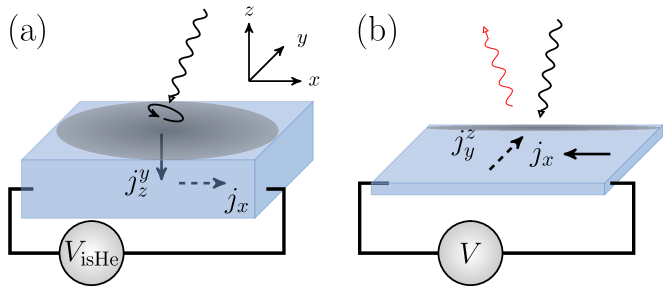
Figure 4: Left panel: A broad spot of circularly polarised light creates a non-equilibrium spin polarisation $\delta s^{y}$ at a sample’s surface (shaded region), and a a diffusion spin current $j^{y}_{z}\sim\partial_{z}\delta s^{y}$ flows into the 3D bulk. Here the isHe generates a transverse charge current $j_{x}$, yielding a finite output voltage $V_{\rm isHe}$. Setups of this kind were proposed already in the early days of spin Hall physics [3]. Right panel: In a 2D system the charge current $j_{x}$ from an applied bias $V$ is converted into a spin Hall current $j^{z}_{y}$. The resulting spin accumulation at the edges (shaded region) is measured by Kerr rotation of scattered light (red). The technique was employed in the first experimental observation of the sHe in a 2D electron gas [54], and a similar one in a 2D hole gas [55]. The connection between bulk spin currents and edge spin accumulations can however be less direct than this cartoon suggests [3, 26, 22, 23, 24].

The numerous experimental schemes available can roughly be divided into three classes.

• Optical setups, historically the first to be used to detect the sHe/isHe, exploit the interaction between polarised light and the spin of charge carriers. For example, circularly polarised light can be used to generate local non-equilibrium spin accumulations which later diffuse through the system. The diffusion spin current can then be converted by the isHe into charge signals measured with standard electrodes, see Fig. 4 (a). On the other hand, spin accumulations can be measured by circularly polarised electroluminescence or magneto-optical Kerr and Faraday effects. An example is shown in Fig. 4 (b), where the spin accumulation at the edge of the system generated by the sHe is measured by the degree of (Kerr) rotation of light scattered off the sample. All-optical schemes are also employed [56, 57], allowing in particular time-resolved experiments on ultra-short (THz) timescales [56] – which are not accessible to electronic systems.

• Magneto-electric (spin pumping, spin torque) setups, relying on the interplay between magnetisation and spin dynamics [58]. Fig. 5 shows a paradigmatic example: a spin current ${\bf j}^{s}_{\rm in}$ is injected from an out-of-equilibrium magnetic element, e.g. a (conducting or insulating) magnet driven by microwaves, and converted into a charge current ${\bf j}^{c}_{\rm out}$ collected at a normal metallic electrode. The latter can actually be used to run the experiment under “reverse bias”: ${\bf j}^{c}_{\rm in}$ is injected, and one measures the torque that the resulting ${\bf j}^{s}_{\rm out}$ exerts on the adjacent magnet. The presence of magnetic elements considerably increases the degree of complexity of the overall system, and may lead to additional effects which are however beyond the scope of this short overview [58, 59]. Time-dependent experiments are also performed, e.g. to measure AC spin Hall effects [60, 61, 62].

• All-electrical setups, conceptually probably the simplest. Fig. 6 (a) shows a most basic one, without any magnetic element: A charge current ${\bf j}^{c}_{\rm in}$ is injected by a metallic electrode, is converted into a spin signal by the sHe, and finally re-converted by the isHe into an outgoing ${\bf j}^{c}_{\rm out}$ collected at some other electrode. A very popular scheme requiring a magnetic electrode is instead sketched in Fig. 6 (b). Both are non-local – input electrodes are somewhere, output electrodes elsewhere – a common feature in spin Hall setups [5, 63].

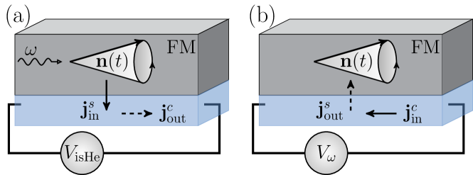
Figure 5: Left panel: Sketch of a spin pumping setup. Microwaves in a ferro-/ferrimagnet FM at frequency $\omega$ drive the magnetisation, ${\bf M}=M{\bf n}\to{{\bf M}(t)=M{\bf n}(t)}$. Its precession injects angular momentum into the underlying spin-orbit coupled normal metal, generating a spin current ${\bf j}^{s}$. The latter is converted by the isHe into a charge current ${\bf j}^{c}$ and ergo a measurable voltage $V_{\rm isHe}$, in general with both DC and AC components [64, 61, 62]. Right panel: A reverse-bias scenario, in which a charge current at frequency $\omega$ is injected and converted by the sHe into an AC spin current. The latter exerts a torque on ${\bf M}$ and drives its precession. There are numerous DC and AC variations to these schemes, involving many different magneto-resistive effects modulated by spin-orbit interaction, see Refs. [8, 11] for an overview.

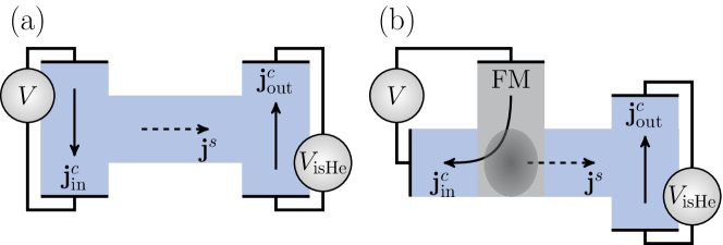
Figure 6: Left panel: Hall bar geometry without magnetic elements. The injected charge current ${\bf j}^{c}_{\rm in}$ is converted into a transverse spin current ${\bf j}_{s}$ by the sHe. The latter is converted back into a charge current ${\bf j}^{c}_{\rm out}$ by the isHe in the right arm of the setup, yielding a finite $V_{\rm isHe}$. One of the earliest implementations of this setup was used to measure the ballistic sHe in a HgTe quantum well [65]. Right panel: non-local setup with a ferromagnetic (FM) electrode, shown in dark grey, deposited on top of a T-shaped metallic film. The injected current ${\bf j}^{c}_{\rm in}$ is drained to the left contact, since the right metallic arm is at the same electrochemical potential as the FM electrode. The current ${\bf j}^{c}_{\rm in}$ is spin polarised, therefore it creates a non-equilibrium spin accumulation underneath the FM contact, shown by the shaded area. Part of it diffuses towards the right, yielding a pure spin current ${\bf j}^{s}$ which is then converted by the isHe into a measurable transverse voltage $V_{\rm isHe}$. The scheme was first employed by Valenzuela and Tinkham [5].

The boundary between classes is clearly blurred, and mixed techniques are often employed. An important general observation is that experimental setups – apart perhaps from the simplest all-electrical ones – are fairly complex, consisting of multiple elements of different nature subject to various kinds of drivings. Paired with the vast number of spin-charge (or charge-spin) conversion channels available in any given system, this makes for interesting debates concerning possible microscopic interpretations of experiments.

IV Theory

IV.1 An instructive example and the general framework

The spin Hall effects are non-equilibrium phenomena handled with the usual arsenal of transport theory techniques: Keldysh formalism, density matrix and semiclassical kinetics, Kubo formula, Landauer-Büttiker formalism …. Irrespective of the techniques employed, a source of substantial theoretical challenges is complexity. In crude terms, the Hamiltonian of a spin Hall system requires numerous ingredients, recall the discussion from Sec. III. The resulting quasiparticle dynamics are in general quite sensitive to the presence/absence of, and competition between, each.

To see this in a concrete way it is instructive to start from the barebone model of an ideal Rashba system

$$H_{\rm R}=\frac{p^{2}}{2m}+\frac{\alpha}{\hbar}\left[p_{y}\sigma^{x}-p_{x}\sigma^{y}\right],$$ (16)

where $m$ is the effective electron mass and $\alpha\sim\nabla V_{\rm int}(z)$ the Rashba coupling constant, proportional to the (effective) electric field confining the electrons to the $x$-$y$ plane – see the heuristic discussion in Sec. II, Eq. (8).

Given $H_{R}$, the goal is to compute the frequency-dependent spin Hall conductivity $\sigma^{\rm sHe}(\omega)$, defined as

$$j^{z}_{y}(\omega)=\sigma^{\rm sHe}(\omega)E_{x}(\omega),$$ (17)

with $j^{z}_{y}$ the $z$-polarised spin current in the $y$ direction. The standard choice is to take the symmetrised spin current definition (14) – other choices are possible, recall the discussion from Sec. II, and the consequences will be addressed below. The spin Hall conductivity can be written in terms of the spin current-charge current Kubo response function $\langle\langle j^{z}_{y};j_{x}\rangle\rangle_{\omega}\equiv-\frac{i}{\hbar}\int_{0}^{t}\left[j^{z}_{y}(t),j_{x}(0)\right]e^{i\omega t}{\rm d}t$, with $[A,B]=AB-BA$ the commutator [70]. Since the charge current couples to the vector potential as ${\bf j}\cdot{\bf A}$, and $E_{x}(\omega)=-i\omega A_{x}(\omega)$, one has

$$\sigma^{\rm sHe}(\omega)=\frac{\langle\langle j^{z}_{y};j_{x}\rangle\rangle_{\omega}}{i\omega}.$$ (18)

Once the DC $\sigma^{\rm sHe}\equiv\lim_{\omega\to 0}\sigma^{\rm sHe}(\omega)$ is known the spin Hall angle follows

$$\theta^{\rm sHe}=\frac{q}{\hbar}\frac{\sigma^{\rm sHe}}{\sigma^{c}_{x}},$$ (19)

with $\sigma^{c}_{x}$ the longitudinal DC charge conductivity. An explicit computation yields the “universal” DC result

$$\sigma^{\rm sHe}_{\rm clean}=\frac{e}{8\pi\hbar},$$ (20)

with the electron charge $q=-e<0$. The subscript “clean” highlights that the system is without any defects. Such a beautiful result, due to the intrinsic Berry phase of electrons on the Rashba Fermi surface, is unfortunately very fragile. If one adds dirt to the model, i.e. a random impurity potential, $H_{\rm R}\to H_{\rm R}+V_{\rm imp}({\bf r})$, the spin Hall conductivity exactly vanishes

$$\sigma^{\rm sHe}_{\rm dirty}=0.$$ (21)

The vanishing is diagrammatically subtle: since it comes from vertex corrections, it cannot be guessed by simply introducing a disorder broadening of the momentum eigenstates in the Kubo response kernel [71, 72, 73]. Indeed, it was overlooked at first in the scientific literature [74]. On the other hand, it is easily understood with kinetic arguments [75, 76], since the homogeneous continuity equation for the $y$-spin component reads

$$\partial_{t}s^{y}=\underbrace{-\frac{2m\alpha}{\hbar^{2}}j^{z}_{y}}_{\Gamma^{y}_{\rm int}}.$$ (22)

At steady state the spin current $j^{z}_{y}=0$.

Eq. (21) is as fragile as its clean counterpart (20). If one further adds extrinsic spin-orbit interaction, that is spin-orbit interaction with the impurity potential, $H_{\rm R}\to H_{\rm R}+V_{\rm imp}({\bf r})+\lambda\mbox{\boldmath$\sigma$}\times\nabla V_{\rm imp}({\bf r})\cdot{\bf p}$, the spin Hall conductivity is non-zero

$$\sigma^{\rm sHe}_{\rm int+ext}\neq 0,$$ (23)

and furthermore depends non-trivially on different system parameters. In particular [37, 38]

$$\sigma^{\rm sHe}_{\rm int+ext}\neq\sigma^{\rm sHe}_{\rm int}+\sigma^{\rm sHe}_{\rm ext}.$$ (24)

Equivalent results would have been reached starting from the (linear) Dresselhaus model

$$H_{D}=\frac{p^{2}}{2m}+\frac{\beta}{\hbar}\left[p_{x}\sigma^{x}-p_{y}\sigma^{y}\right],$$ (25)

where the coupling constant $\beta$ is now due to bulk inversion asymmetry, i.e. the lack of inversion symmetry of the underlying crystal, as in zincblend compounds [15].

The lesson to be learned from this example is not that low-energy effective models of Rashba or Dresselhaus type are unreliable – quite the contrary, they are pillars of spintronics, even if more complex models are often needed e.g. for precise quantitative comparisons with experiments. It is rather that any effect crucially depending on the coupling between orbital motion and internal (spin) dynamics is subtler than standard charge-only transport phenomena, even when their description is based on the simplest models. As a corollary, attacking the problem from different angles – Kubo vs. kinetics in this case – can be a good idea.

The Rashba and Dresselhaus scenarios just considered are examples of a standard approach to transport widely employed throughout condensed matter. The latter starts from some low-energy (${\bf k}\cdot{\bf p}$) effective model whose parameters can be computed with ab-initio methods, or left as symmetry-allowed parameters to be estimated by comparison with experiments. In our case the minimal Hamiltonian for spin 1/2 quasiparticles reads

$$H=H_{0}+{\bf b}({\bf p})\cdot\mbox{\boldmath$\sigma$}+\delta H$$ (26)

where $H_{0}$ describes band-bottom (top) free electrons (holes), and ${\bf b}({\bf p})$ is the effective intrinsic spin-orbit field, see Eq. (10). Higher-dimensional models (4 x 4, 6 x 6 …) are employed whenever more than a single $s$-band lie close to the Fermi energy, which is the case e.g. for graphene [77, 78, 79, 80], Pt [81] or typically for holes [15, 4]. On the other hand there are situations in which the term ${\bf b}({\bf p})$ is negligible, e.g. in bulk Al or Cu. The last term $\delta H$ contains all extra ingredients needed in the specific situation, e.g. exchange coupling with a magnetic texture, extrinsic spin-orbit coupling, disorder, phonons and so on.

The effective Hamiltonian (26) is used to study non-equilibrium dynamics with whatever analytical and/or numerical techniques one prefers. The approach is thus very general and flexible. Alternatively, it is also possible to stick to ab-initio methods and use an atomistic Hamiltonian throughout. In this case one typically relies on Kubo linear response formalism to compute the relevant transport coefficients, e.g. $\sigma^{\rm sHe}$ [82, 83].

IV.2 Onsager reciprocity and a non-Abelian gauge field point of view

The sHe and isHe connect spin currents, even under time-reversal, with charge currents, odd under time-reversal. From the general properties of Kubo response functions [70] there follows

$$\langle\langle j^{z}_{y};j_{x}\rangle\rangle_{\omega}=-\langle\langle j_{x};j^{z}_{y}\rangle\rangle_{\omega},$$ (27)

which implies

$$\sigma^{\rm sHe}=-\sigma^{\rm isHe}.$$ (28)

This is the (linear response) Onsager relation between the sHe and isHe. It is evident that changing the definition of the spin current changes the value of $\sigma^{\rm sHe}$ and $\sigma^{\rm isHe}$. This is critical if a direct comparison with experiments is seeked: what spin current is being excited in the experimental setup? What spin Hall angle are we talking about? As discussed in Sec. (II) there are numerous ways to remove any ambiguity from such a comparison. In particular, if one is not interested in local quantities such as conductivities, the problem can be bypassed by considering conductances between metallic leads without spin-orbit interaction [32]. On the other hand a change of spin current definition does not break Onsager reciprocity if done consistently, i.e. if the same definition is used to describe both the direct, say sHe, and reverse bias, say isHe, scenario.

Another source of concern in the early 2000s was that the standard definition of spin currents, Eq. (14), may yield non-vanishing equilibrium (circulating) currents [25]. Different authors highlighted however that there is nothing intrinsically unphysical or surprising in this [84, 29]: spin currents are even under time-reversal, so can exist in equilibrium, and physical systems hosting different kinds of equilibrium currents anyway exist [85, 84, 29, 30]. Indeed, adopting a non-Abelian gauge field point of view, equilibrium spin currents can be identified with the non-Abelian analogous of dissipationless Landau paramagnetic currents in solids [29].

The non-Abelian gauge field approach requires to rewrite the spin-orbit interaction in terms of a non-Abelian vector potential ${\bm{\mathcal{A}}}$, i.e. a tensor ${\cal A}^{a}_{i}$ with both spin $(a)$ and real space $(i)$ indices. To be definite, for the Rashba Hamiltonian (16) one has

$$H_{R}=\frac{\left({\bf p}+{\bm{\mathcal{A}}}\right)^{2}}{2m}+{\rm const.}$$ (29)

with ${\cal A}^{y}_{x}=-{\cal A}^{x}_{y}=2m\alpha/\hbar^{2}$, while ${\cal A}^{a}_{j}=0$ for all other components. The spin current immediately follows from $j^{a}_{i}=\partial H_{R}/\partial{\cal A}^{a}_{i}$. It coincides with the standard definition (14) and generally consists of both transport contributions and a non-dissipative equilibrium part. Pursuing this route e.g. in a diffusive sample, one obtains in particular a clear parallel between the standard Hall current ${\bf j}_{\rm Hall}$ in presence of a magnetic field ${\bf B}$ and the $a$-polarised spin Hall current ${\bf j}^{a}_{\rm sHe}$ in presence of a non-Abelian pseudomagnetic field ${\bm{\mathcal{B}}}$ generated by ${\bm{\mathcal{A}}}$ [36]

$${\bf j}_{\rm Hall}=\frac{q\tau}{m}{\bf j}\times{\bf B}\;\to\;{\bf j}^{a}_{\rm sHe}=\frac{q\tau}{4m}{\bf j}\times{\bm{\mathcal{B}}}^{a}.$$ (30)

The non-Abelian gauge field approach is based on relatively old ideas [86, 87, 88], but was recently revived to describe spin-charge coupled transport in different settings [36, 38, 89, 90, 91, 92, 93, 94, 95, 96, 97]. While its merits are evident, one should realise that a rewriting like Eq. (29) is not always possible. I refer to the relevant literature for details.

V Conclusions

The spin Hall effects are a family of transverse transport phenomena appearing in (pseudo)spin-orbit coupled systems. A good chunk of the theory and experimental background was established in the 1970s-1980s, but the effects became widely known in condensed matter only starting from the early 2000s, and are nowadays cornerstones of both fundamental and applied spintronic research. Such a late blooming is probably due in good part to two roughly contemporary events. First, the widespread realisation of the importance of geometry/topology-related concepts for Bloch electrons. Since the latter usually require quasiparticles to have an internal structure, this strongly increased interest for (pseudo)spin-orbit coupled dynamics. Second, technological advances which notably allowed the fabrication of high-quality semiconductor heterostructures, where spin manipulation became possible with a high level of precision, soon after followed by the discovery and functionalisation of graphene and other materials with strong (pseudo)spin-orbit interaction.

In this short overview I focused on the core, standard forms of the spin Hall effects, as they exist in normal Fermi liquids. In this context they are active in a wide range of parameters, from large samples at room temperature – important for potential applications – down to mesoscopic samples at low temperatures. However they may also appear in e.g. strongly disordered systems [98], superconductors [99], metallic antiferromagnets [100, 101], as “valley Hall effects” in different materials [102, 103, 104] or in the propagation of magnons [105, 106] and light [107]. They may also contribute to other transport effects, such as the spin Hall magnetoresistance [108, 109, 110]. In short, they are potentially present in any scenario where transport is due to quasiparticles with some internal structure which couples to a non-trivial background.

V.1 Notes on further readings

The literature on the spin Hall effects is vast and ramifies quickly to neighbouring subfields. The bibliography given here is meant to provide barebone directions to the newcomer, but is by no means exhaustive. Numerous review articles, each with its own qualities and shortcomings, are available to the interested reader. Refs. [3] and [4] are both must-read works. Ref. [3] provides in particular a thorough historical overview and excellent phenomenological discussions, while Ref. [4] offers a high-quality and very compact introduction to the technical background, introducing also modern topological concepts. I also suggest Ref. [11] for a recent, short and more application-oriented discussion, and Ref. [111] for its theory part. Finally, Ref. [8] provides an excellent experimental overview.

VI Acknowledgements

I am indebted to Lin Chen for a careful reading of the manuscript, and to Leonid E. Golub for useful comments. I also thank all STherQO members for discussions, in particular Guillaume Weick and Rémy Dubertrand.

References

- Dyakonov and Perel [1971] M. I. Dyakonov and V. I. Perel, Current-induced spin orientation of electrons in semiconductors, Phys. Lett. A 35, 459 (1971).
- Hirsch [1999] J. E. Hirsch, Spin hall effect, Phys. Rev. Lett. 83, 1834 (1999).
- Dyakonov and Khaetskii [2006] M. I. Dyakonov and A. V. Khaetskii, Spin hall effect, in Spin Physics in Semiconductors (Springer, 2006) p. 211.
- Engel et al. [2007] H.-A. Engel, E. I. Rashba, and B. I. Halperin, Theory of spin hall effects in semiconductors, in Handbook of Magnetism and Advanced Magnetic Materials (John Wiley & Sons, 2007) p. 2858.
- Valenzuela and Tinkham [2006] S. O. Valenzuela and M. Tinkham, Direct electronic measurement of the spin hall effect, Nature 442, 176 (2006).
- Hahn et al. [2013a] C. Hahn, G. de Loubens, O. Klein, M. Viret, V. V. Naletov, and J. Ben Youssef, Comparative measurements of inverse spin hall effects and magnetoresistance in yig/pt and yig/ta, Phys. Rev. B 87, 174417 (2013a).
- Obstbaum et al. [2014] M. Obstbaum, M. Härtinger, H. G. Bauer, T. Meier, F. Swientek, C. H. Back, and G. Woltersdorf, Inverse spin hall effect in /normal-metal bilayers, Phys. Rev. B 89, 060407(R) (2014).
- Sinova et al. [2015] J. Sinova, S. O. Valenzuela, J. Wunderlich, C. H. Back, and T. Jungwirth, Spin hall effects, Rev. Mod. Phys. 87, 1213 (2015).
- Hasan and Kane [2010] M. Z. Hasan and C. L. Kane, Topological insulators, Rev. Mod. Phys. 82, 3045 (2010).
- König et al. [2007] M. König, S. Wiedmann, C. Brüne, A. Roth, H. Buhmann, L. W. Molenkamp, X.-L. Qi, and S.-C. Zhang, Quantum spin hall insulator state in hgte quantum wells, Science 318, 766 (2007).
- Fert and Dau [2019] A. Fert and F. N. V. Dau, Spintronics, from giant magnetoresistance to magnetic skyrmions and topological insulators, C. R. Physique 20, 817 (2019).
- Nagaosa et al. [2010] N. Nagaosa, J. Sinova, S. Onoda, A. H. MacDonald, and N. P. Ong, Anomalous hall effect, Rev. Mod. Phys. 82, 1539 (2010).
- Culcer et al. [2010] D. Culcer, E. M. Hankiewicz, G. Vignale, and R. Winkler, Side jumps in the spin hall effect: Construction of the boltzmann collision integral, Phys. Rev. B 81, 125332 (2010).
- Bychkov and Rashba [1984] Y. A. Bychkov and E. I. Rashba, JETP Lett. 39, 78 (1984).
- Winkler [2003] R. Winkler, Spin-Orbit Coupling Effects in Two-Dimensional Electron and Hole Systems (Springe, 2003).
- Gorini et al. [2015] C. Gorini, U. Eckern, and R. Raimondi, Spin hall effects due to phonon skew scattering, Phys. Rev. Lett. 115, 076602 (2015).
- Karnad et al. [2018] G. V. Karnad, C. Gorini, K. Lee, T. Schulz, R. L. Conte, A. W. J. Wells, D.-S. Han, K. Shahbazi, J.-S. Kim, T. A. Moore, H. J. M. Swagten, U. Eckern, R. Raimondi, and M. Kläui, Evidence for phonon skew scattering in the spin hall effect of platinum, Phys. Rev. B 97, 100405 (2018).
- Okamoto et al. [2019] S. Okamoto, T. Egami, and N. Nagaosa, Critical spin fluctuation mechanism for the spin hall effect, Phys. Rev. Lett. 123, 196603 (2019).
- Ohnuma et al. [2016] Y. Ohnuma, M. Matsuo, and S. Maekawa, Spin transport in half-metallic ferromagnets, Phys. Rev. B 94, 184405 (2016).
- Dugaev et al. [2010] V. K. Dugaev, M. Inglot, E. Y. Sherman, and J. Barnaś, Robust impurity-scattering spin hall effect in a two-dimensional electron gas, Phys. Rev. B 82, 121310(R) (2010).
- Sonin [2007a] E. B. Sonin, Proposal for measuring mechanically equilibrium spin currents in the rashba medium, Phys. Rev. Lett. 99, 266602 (2007a).
- Adagideli et al. [2007] I. Adagideli, M. Scheid, M. Wimmer, G. E. W. Bauer, and K. Richter, Extracting current-induced spins: spin boundary conditions at narrow hall contacts, New J. Phys. 9, 382 (2007).
- Sonin [2010a] E. B. Sonin, Edge spin accumulation: Spin hall effect without bulk spin current, Phys. Rev. B 81, 113304 (2010a).
- Gorini et al. [2012] C. Gorini, R. Raimondi, and P. Schwab, Onsager relations in a two-dimensional electron gas with spin-orbit coupling, Phys. Rev. Lett. 109, 246604 (2012).
- Rashba [2003] E. I. Rashba, Spin currents in thermodynamic equilibrium: The challenge of discerning transport currents, Phys. Rev. B 68, 241315(R) (2003).
- Nikolić et al. [2006] B. K. Nikolić, L. P. Zârbo, and S. Souma, Imaging mesoscopic spin hall flow: Spatial distribution of local spin currents and spin densities in and out of multiterminal spin-orbit coupled semiconductor nanostructures, Phys. Rev. B 73, 075303 (2006).
- Shi et al. [2006] J. Shi, P. Zhang, D. Xiao, and Q. Niu, Phys. Rev. Lett. 96, 076604 (2006).
- Sugimoto et al. [2006] N. Sugimoto, S. Onoda, S. Murakami, and N. Nagaosa, Spin hall effect of a conserved current: Conditions for a nonzero spin hall current, Phys. Rev. B 73, 113305 (2006).
- Tokatly [2008] I. V. Tokatly, Equilibrium spin currents: Non-abelian gauge invariance and color diamagnetism in condensed matter, Phys. Rev. Lett. 101, 106601 (2008).
- Sonin [2010b] E. B. Sonin, Spin currents and spin superfluidity, Advances in Physics 59, 181 (2010b).
- Khaetskii [2014] A. Khaetskii, Edge spin accumulation in two-dimensional electron and hole systems in a quasiballistic regime, Phys. Rev. B 89, 195408 (2014).
- Jacquod et al. [2012] P. Jacquod, R. Whitney, J. Meair, and M. Büttiker, Onsager relations in coupled electric, thermoelectric and spin transport: The ten-fold way, Phys. Rev. B 86, 155118 (2012).
- Burkov et al. [2004] A. A. Burkov, S. Núnez, and A. H. MacDonald, Theory of spin-charge-coupled transport in a two-dimensional electron gas with rashba spin-orbit interactions, Phys. Rev. B 70, 155308 (2004).
- Mal’shukov et al. [2005] A. G. Mal’shukov, L. Y. Wang, C. S. Chu, and K. A. Chao, Spin hall effect on edge magnetization and electric conductance of a 2d semiconductor strip, Phys. Rev. Lett. 95, 146601 (2005).
- Raimondi et al. [2006] R. Raimondi, C. Gorini, P. Schwab, and M. Dzierzawa, Quasiclassical approach to the spin hall effect in the two-dimensional electron gas, Phys. Rev. B 74, 035340 (2006).
- Gorini et al. [2010] C. Gorini, P. Schwab, R. Raimondi, and A. L. Shelankov, Non-abelian gauge fields in the gradient expansion: Generalized boltzmann and eilenberger equations, Phys. Rev. B 82, 195316 (2010).
- Raimondi and Schwab [2009] R. Raimondi and P. Schwab, Tuning the spin hall effect in a two-dimensional electron gas, EPL (Europhysics Letters) 87, 37008 (2009).
- Raimondi et al. [2012] R. Raimondi, P. Schwab, C. Gorini, and G. Vignale, Spin-orbit interaction in a two-dimensional electron gas: formulation, Ann. Phys. (Berlin) 524, 153 (2012).
- Adagideli and Bauer [2005] I. Adagideli and G. E. W. Bauer, Intrinsic spin hall edges, Phys. Rev. Lett. 95, 256602 (2005).
- Tserkovnyak et al. [2007] Y. Tserkovnyak, B. I. Halperin, A. A. Kovalev, and A. Brataas, Boundary spin hall effect in a two-dimensional semiconductor system with rashba spin-orbit coupling, Phys. Rev. B 76, 085319 (2007).
- Mal’shukov et al. [2007] A. G. Mal’shukov, L. Y. Wang, and C. S. Chu, Spin-hall interface resistance in terms of landauer-type spin dipoles, Phys. Rev. B 78, 085315 (2007).
- Amin and Stiles [2016] V. P. Amin and M. D. Stiles, Spin transport at interfaces with spin-orbit coupling: Formalism, Phys. Rev. B 94, 104419 (2016).
- Tölle et al. [2018] S. Tölle, M. Dzierzawa, U. Eckern, and C. Gorini, Quasiclassical theory of the spin–orbit magnetoresistance of three-dimensional rashba metals, New J. Phys. 20, 103024 (2018).
- Zhu et al. [2019] L. Zhu, L. Zhu, M. Sui, D. C. Ralph, and R. A. Buhrman, Variation of the giant intrinsic spin hall conductivity of pt with carrier lifetime, Science Advances 5, eaav8025 (2019).
- Nakagawara et al. [2019] K. Nakagawara, S. Kasai, J. Ryu, S. Mitani, L. Liu, M. Kohda, and J. Nitta, Temperature-dependent spin hall effect tunneling spectroscopy in platinum, Appl. Phys. Lett. 115, 162403 (2019).
- Li et al. [2021] P. Li, L. J. Riddiford, C. Bi, J. J. Wisser, X.-Q. Sun, A. Vailionis, M. J. Veit, A. Altman, X. Li, M. DC, S. X. Wang, Y. Suzuki, and S. Emori, Charge-spin interconversion in epitaxial pt probed by spin-orbit torques in a magnetic insulator, Phys. Rev. Materials 5, 064404 (2021).
- Yanez et al. [2021] W. Yanez, Y. Ou, R. Xiao, J. Koo, J. T. Held, S. Ghosh, J. Rable, T. Pillsbury, E. G. Delgado, K. Yang, J. Chamorro, A. J. Grutter, P. Quarterman, A. Richardella, A. Sengupta, T. McQueen, J. A. Borchers, K. A. Mkhoyan, B. Yan, and N. Samarth, Spin and charge interconversion in dirac-semimetal thin films, Phys. Rev. Applied 16, 054031 (2021).
- Boventer et al. [2021] I. Boventer, H. Simensen, A. Anane, M. Kläui, A. Brataas, and R. Lebrun, Room-temperature antiferromagnetic resonance and inverse spin-hall voltage in canted antiferromagnets, Phys. Rev. Lett. 126, 187201 (2021).
- Liu et al. [2012] L. Liu, O. J. Lee, T. J. Gudmundsen, D. C. Ralph, and R. A. Buhrman, Current-induced switching of perpendicularly magnetized magnetic layers using spin torque from the spin hall effect, Phys. Rev. Lett. 109, 096602 (2012).
- Safeer et al. [2020] C. K. Safeer, J. Ingla-Aynés, N. Ontoso, F. Herling, W. Yan, L. E. Hueso, and F. Casanova, Spin hall effect in bilayer graphene combined with an insulator up to room temperature, Nano Lett. 20, 4573 (2020).
- Karube et al. [2020] S. Karube, D. Sugawara, C. Tang, T. Tanabe, Y. Oyama, and J. Nitta, Enhancement of spin-charge current interconversion by oxidation of rhenium, J. Magn. Magn. Mater. 516, 167298 (2020).
- Rojas-Sánchez et al. [2014] J.-C. Rojas-Sánchez, N. Reyren, P. Laczkowski, W. Savero, J.-P. Attané, C. Deranlot, M. Jamet, J.-M. George, L. Vila, and H. Jaffrès, Spin pumping and inverse spin hall effect in platinum: The essential role of spin-memory loss at metallic interfaces, Phys. Rev. Lett. 112, 106602 (2014).
- Pai et al. [2012] C.-F. Pai, L. Liu, Y. Li, H. W. Tseng, D. C. Ralph, and R. A. Buhrman, Spin transfer torque devices utilizing the giant spin hall effect of tungsten, Appl. Phys. Lett. 101, 122404 (2012).
- Kato et al. [2004] Y. K. Kato, R. C. Myers, A. C. Gossard, and D. D. Awschalom, Observation of the spin hall effect in semiconductors, Science 306, 1910 (2004).
- Wunderlich et al. [2005] J. Wunderlich, B. Kaestner, J. Sinova, and T. Jungwirth, Experimental observation of the spin-hall effect in a two-dimensional spin-orbit coupled semiconductor system, Phys. Rev. Lett. 94, 047204 (2005).
- Werake et al. [2011] L. K. Werake, B. A. Ruzicka, and H. Zhao, Observation of intrinsic inverse spin hall effect, Phys. Rev. Lett. 106, 107205 (2011).
- Seifert et al. [2016] T. Seifert, S. Jaiswal, U. Martens, J. Hannegan, L. Braun, P. Maldonado, F. Freimuth, A. Kronenberg, J. Henrizi, I. Radu, E. Beaurepaire, Y. Mokrousov, P. M. Oppeneer, M. Jourdan, G. Jakob, D. Turchinovich, L. M. Hayden, M. Wolf, M. Münzenberg, M. Kläui, and T. Kampfrath, Efficient metallic spintronic emitters of ultrabroadband terahertz radiation, Nat. Photon. 10, 483 (2016).
- Tserkovnyak et al. [2005] Y. Tserkovnyak, A. Brataas, G. E. W. Bauer, and B. I. Halperin, Nonlocal magnetization dynamics in ferromagnetic heterostructures, Rev. Mod. Phys. 77, 1375 (2005).
- Manchon et al. [2019] A. Manchon, J. Z̆elezný, I. M. Miron, T. Jungwirth, J. Sinova, A. Thiaville, K. Garello, and P. Gambardella, Current-induced spin-orbit torques in ferromagnetic and antiferromagnetic systems, Rev. Mod. Phys. 91, 035004 (2019).
- Hahn et al. [2013b] C. Hahn, G. de Loubens, M. Viret, O. Klein, V. V. Naletov, and J. B. Youssef, Phys. Rev. Lett. 111, 217204 (2013b).
- Wei et al. [2014] D. Wei, M. Obstbaum, M. Ribow, C. H. Back, and G. Woltersdorf, Spin hall voltages from a.c. and d.c. spin currents, Nat. Comms. 5, 3768 (2014).
- Weiler et al. [2014] M. Weiler, J. M. Shaw, H. T. Nembach, and T. J. Silva, Phase-sensitive detection of spin pumping via the ac inverse spin hall effect, Phys. Rev. Lett. 113, 157204 (2014).
- Takahashi and Maekawa [2007] S. Takahashi and S. Maekawa, Nonlocal spin hall effect and spin–orbit interaction in nonmagnetic metals, J. Magn. Magn. Mater. 310, 2067 (2007).
- Jiao and Bauer [2013] H. Jiao and G. E. W. Bauer, Spin backflow and ac voltage generation by spin pumping and the inverse spin hall effect, Phys. Rev. Lett. 110, 217602 (2013).
- Brüne et al. [2010] C. Brüne, A. Roth, E. G. Novik, M. König, H. Buhmann, E. M. Hankiewicz, W. Hanke, J. Sinova, and L. W. Molenkamp, Evidence for the ballistic intrinsic spin hall effect in hgte nanostructures, Nature Phys. 6, 448 (2010).
- Ganichev et al. [2002] S. D. Ganichev, E. L. Ivchenko, V. V. Bel’kov, S. A. Tarasenko, M. Sollinger, D. Weiss, W. Wegscheider, and W. Prettl, Spin-galvanic effect, Nature 417, 153 (2002).
- [67] S. D. Ganichev, M. Trushin, and J. Schliemann, Spin polarisation by current, arXiv , 1606.02043.
- Shen et al. [2014] K. Shen, R. Raimondi, and G. Vignale, Microscopic theory of the inverse edelstein effect, Phys. Rev. Lett. 112, 096601 (2014).
- Gorini et al. [2017] C. Gorini, A. M. Sheikhabad, K. Shen, I. V. Tokatly, G. Vignale, and R. Raimondi, Theory of current-induced spin polarization in an electron gas, Phys. Rev. B 95, 205424 (2017).
- Landau et al. [2008] L. D. Landau, E. M. Lifschitz, and L. P. Pitaevskii, Electrodynamics of Continuous Media (Elsevier, 2008).
- Schwab and Raimondi [2002] P. Schwab and R. Raimondi, Magnetoconductance of a two-dimensional metal in the presence of spin-orbit coupling, Eur. Phys. J. B 25, 483 (2002).
- Inoue et al. [2004] J.-I. Inoue, G. E. W. Bauer, and L. W. Molenkamp, Suppression of the persistent spin hall current by defect scattering, Phys. Rev. B 70, 041303(R) (2004).
- Raimondi and Schwab [2005] R. Raimondi and P. Schwab, Spin-hall effect in a disordered two-dimensional electron system, Phys. Rev. B 71, 033311 (2005).
- Sinova et al. [2004] J. Sinova, D. Culcer, Q. Niu, N. A. Sinitsyn, T. Jungwirth, and A. H. MacDonald, Universal intrinsic spin hall effect, Phys. Rev. Lett. 92, 126603 (2004).
- Dimitrova [2005] O. V. Dimitrova, Spin-hall conductivity in a two-dimensional rashba electron gas, Phys. Rev. B 71, 245327 (2005).
- Chalaev and Loss [2005] O. Chalaev and D. Loss, Spin-hall conductivity due to rashba spin-orbit interaction in disordered systems, Phys. Rev. B 71, 245318 (2005).
- Neto et al. [2009] A. H. C. Neto, F. Guinea, N. M. R. Peres, K. S. Novoselov, and A. K. Geim, The electronic properties of graphene, Rev. Mod. Phys. 81, 109 (2009).
- Kochan et al. [2017] D. Kochan, S. Irmer, and J. Fabian, Model spin-orbit coupling hamiltonians for graphene systems, Phys. Rev. B 95, 165415 (2017).
- Dyrdał and Barnaś [2012] A. Dyrdał and J. Barnaś, Spin hall effect in graphene due to random rashba field, Phys. Rev. B 86, 161401(R) (2012).
- Milletarí et al. [2017] M. Milletarí, M. Offidani, A. Ferreira, and R. Raimondi, Covariant conservation laws and the spin hall effect in dirac-rashba systems, Phys. Rev. Lett. 119, 246801 (2017).
- Guo et al. [2008] G. Y. Guo, S. Murakami, T.-W. Chen, and N. Nagaosa, Intrinsic spin hall effect in platinum: First-principles calculations, Phys. Rev. Lett. 100, 096401 (2008).
- Lowitzer et al. [2011] S. Lowitzer, M. Gradhand, D. Ködderitzsch, D. V. Fedorov, I. Mertig, and H. Ebert, Extrinsic and intrinsic contributions to the spin hall effect of alloys, Phys. Rev. Lett. 106, 056601 (2011).
- Ködderitzsch et al. [2015] D. Ködderitzsch, K. Chadova, and H. Ebert, Linear response kubo-bastin formalism with application to the anomalous and spin hall effects: A first-principles approach, Phys. Rev. B 92, 184415 (2015).
- Sonin [2007b] E. B. Sonin, Phys. Rev. B 76, 033306 (2007b).
- Heurich et al. [2003] J. Heurich, J. König, and A. H. MacDonald, Persistent spin currents in helimagnets, Phys. Rev. B 68, 064406 (2003).
- Mathur and Stone [1992] H. Mathur and A. D. Stone, Quantum transport and the electronic aharonov-casher effect, Phys. Rev. Lett. 68, 2964 (1992).
- Fröhlich and Studer [1993] J. Fröhlich and U. M. Studer, Gauge invariance and current algebra in nonrelativistic many-body theory, Rev. Mod. Phys. 65, 733 (1993).
- Brouwer et al. [2002] P. W. Brouwer, J. N. H. J. Cremers, and B. I. Halperin, Weak localization and conductance fluctuations of a chaotic quantum dot with tunable spin-orbit coupling, Phys. Rev. B 65, 081302(R) (2002).
- Adagideli et al. [2012] I. Adagideli, V. Lutsker, M. Scheid, P. Jacquod, and K. Richter, Spin transistor action from hidden onsager reciprocity, Phys. Rev. Lett. 108, 236601 (2012).
- Bergeret and Tokatly [2013] F. S. Bergeret and I. V. Tokatly, Singlet-triplet conversion and the long-range proximity effect in superconductor-ferromagnet structures with generic spin dependent fields, Phys. Rev. Lett. 110, 117003 (2013).
- Tokatly and Sherman [2016] I. V. Tokatly and E. Y. Sherman, Spin evolution of cold atomic gases in fields, Phys. Rev. A 93, 063635 (2016).
- Tölle et al. [2017] S. Tölle, U. Eckern, and C. Gorini, Spin-charge coupled dynamics driven by a time-dependent magnetization, Phys. Rev. B 95, 115404 (2017).
- Bobkova and Bobkov [2017] I. V. Bobkova and A. M. Bobkov, Quasiclassical theory of magnetoelectric effects in superconducting heterostructures in the presence of spin-orbit coupling, Phys. Rev. B 95, 184518 (2017).
- Jacobsen and Linder [2017] S. H. Jacobsen and J. Linder, Quantum kinetic equations and anomalous nonequilibrium cooper-pair spin accumulation in rashba wires with zeeman splitting, Phys. Rev. B 96, 134513 (2017).
- Mal’shukov [2017] A. G. Mal’shukov, Supercurrent generation by spin injection in an s-wave superconductor–rashba metal bilayer, Phys. Rev. B 95, 064517 (2017).
- Aikebaier et al. [2019] F. Aikebaier, P. Virtanen, and T. Heikkilä, Superconductivity near a magnetic domain wall, Phys. Rev. B 99, 104504 (2019).
- König and Levchenko [2021] E. J. König and A. Levchenko, Quantum kinetics of anomalous and nonlinear hall effects in topological semimetals, Ann. Phys. (New York) 435, 168492 (2021).
- Smirnov and Golub [2017] D. S. Smirnov and L. E. Golub, Electrical spin orientation, spin-galvanic, and spin-hall effects in disordered two-dimensional systems, Phys. Rev. Lett. 118, 116801 (2017).
- Takahashi and Maekawa [2011] S. Takahashi and S. Maekawa, Spin hall effect in superconductors, Jpn. J. Appl. Phys. 51, 010110 (2011).
- Zhang et al. [2014] W. Zhang, M. B. Jungfleisch, W. Jiang, J. E. Pearson, A. Hoffmann, F. Freimuth, and A. Mokrousov, Spin hall effects in metallic antiferromagnets, Phys. Rev. Lett. 113, 196602 (2014).
- Gulbrandsen et al. [2020] S. A. Gulbrandsen, C. Espedal, and A. Brataas, Spin hall effect in antiferromagnets, Phys. Rev. B 101, 184411 (2020).
- Gorbachev et al. [2014] R. V. Gorbachev, J. C. W. Song, G. L. Yu, A. V. Kretinin, F. Withers, Y. Cao, A. Mishchenko, I. V. Grigorieva, K. S. Novoselov, L. S. Levitov, and A. K. Geim, Detecting topological currents in graphene superlattices, Science 346, 448 (2014).
- Mak et al. [2014] K. F. Mak, K. L. McGill, J. Parkand, and P. L. McEuen, The valley hall effect in transistors, Science 344, 1489 (2014).
- Lensky et al. [2015] Y. D. Lensky, J. C. Song, P. Samutpraphoot, and L. S. Levitov, Topological valley currents in gapped dirac materials, Phys. Rev. Lett. 114, 256601 (2015).
- Onose et al. [2010] Y. Onose, T. Ideue, H. Katsura, Y. Shiomi, N. Nagaosa, and Y. Tokura, Observation of the magnon hall effect, Science 329, 297 (2010).
- Mook et al. [2014] A. Mook, J. Henk, and I. Mertig, Magnon hall effect and topology in kagome lattices: A theoretical investigation, Phys. Rev. B 89, 134409 (2014).
- Hosten and Kwiat [2008] O. Hosten and P. Kwiat, Observation of the spin hall effect of light via weak measurements, Science 319, 787 (2008).
- Chen et al. [2016] Y.-T. Chen, S. Takahashi, H. Nakayama, M. Althammer, S. B. T. Goennenwein, E. Saitoh, and G. E. W. Bauer, Theory of spin hall magnetoresistance (smr) and related phenomena, J. Phys.: Condens. Matter 28, 103004 (2016).
- Oyanagi et al. [2021] K. Oyanagi, J. M. Gomez-Perez, X.-P. Zhang, T. Kikkawa, Y. Chen, E. Sagasta, A. Chuvilin, L. E. Hueso, V. N. Golovach, F. S. Bergeret, F. Casanova, and E. Saitoh, Paramagnetic spin hall magnetoresistance, Phys. Rev. B 104, 134428 (2021).
- Chen et al. [2013] L. Chen, F. Matsukura, and H. Ohno, Direct-current voltages in (ga,mn)as structures induced by ferromagnetic resonance, Nat. Commun. 4, 2055 (2013).
- Vignale [2010] G. Vignale, Ten years of spin hall effect, J. Supercond. Nov. Magn. 23, 3 (2010).