Channel Simulation: Finite Blocklengths and Broadcast Channels

Abstract

We study channel simulation under common randomness-assistance in the finite-blocklength regime and identify the smooth channel max-information as a linear program one-shot converse on the minimal simulation cost for fixed error tolerance. We show that this one-shot converse can be achieved exactly using no-signaling assisted codes, and approximately achieved using common randomness-assisted codes. Our one-shot converse thus takes on an analogous role to the celebrated meta-converse in the complementary problem of channel coding, and find tight relations between these two bounds. We asymptotically expand our bounds on the simulation cost for discrete memoryless channels, leading to the second-order as well as the moderate deviation rate expansion, which can be expressed in terms of the channel capacity and channel dispersion known from noisy channel coding. Our techniques extend to discrete memoryless broadcast channels. In stark contrast to the elusive broadcast channel capacity problem, we show that the reverse problem of broadcast channel simulation under common randomness-assistance allows for an efficiently computable single-letter characterization of the asymptotic rate region in terms of the broadcast channel’s multi-partite mutual information. Finally, we present a Blahut–Arimoto type algorithm to compute the rate region efficiently.

I Introduction

Channel simulation is the art of simulating the input-output conditional distribution of a target channel using a noiseless resource channel [2, 3]. Given a target discrete memoryless channel $W_{\mathsf{Y}|\mathsf{X}}$ and using unlimited common randomness, we want to approximately simulate a system that, upon accepting an input $x$ at the receiver, outputs $\mathsf{Y}$ distributed according to the law $W_{\mathsf{Y}|\mathsf{X}}(\cdot|x)$. In other words, we want to simulate the input-output correlations of the channel $W_{\mathsf{Y}|\mathsf{X}}$ as a black-box, using the common randomness and limited communication between sender and receiver. The goal is to find the minimal amount of communication needed to perform this task. Related problems have been studied in the literature under different names, starting with Wyner’s common information [4], channel resolvability [5], strong coordination [6], communication complexity of correlation [7], and channel synthesis [8, 9]. The main difference between these and the model we study here (apart from the availability of unlimited shared randomness) is that channel simulation requires simulation of the channel under arbitrary (i.e., worst-case) inputs whereas in most other studied models the input distribution is fixed. This is remarked upon in [10, Footnote 17]. Notable exceptions include [5, 7]; we will discuss the differences between our model of channel simulation and related works in more detail at the end of this introduction, after we formally introduce our model and discuss our contributions.

I-A Overview of Results

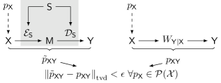
Figure 1: The task of point-to-point channel simulation with the help of common randomness under the worst case error criteria given by the channel TVD defined in (2).

Let us now formally introduce the channel simulation problem (see also Fig. 1). Given a DMC $W_{\mathsf{Y}|\mathsf{X}}$ and a shared random variable $\mathsf{S}$ distributed on some discrete set $\mathcal{S}$, the task of simulating $W_{\mathsf{Y}|\mathsf{X}}$ is to find a set of encoders $\mathcal{E}_{s}\in\mathcal{P}(\{1,\ldots,M\}|\mathcal{X})$ and decoders $\mathcal{D}_{s}\in\mathcal{P}(\mathcal{Y}|\{1,\ldots,M\})$ for each $s\in\mathcal{S}$ such that, the induced channel

$$\widetilde{W}_{\mathsf{Y}|\mathsf{X}}(y|x)\coloneqq\sum_{s\in\mathcal{S}}p_{\mathsf{S}}(s)\cdot\sum_{m\in\{1,\ldots,M\}}\mathcal{E}_{s}(m|x)\cdot\mathcal{D}_{s}(y|m)$$ (1)

is $\epsilon$-close to the channel $W_{\mathsf{Y}|\mathsf{X}}$ within a tolerance of $\epsilon\in[0,1]$ measured in the total variation distance (TVD) (see (2)). Here and in the following, $\mathcal{P}(\mathcal{A}|\mathcal{B})$ denotes the set of all conditional probability distributions on $\mathcal{A}$ conditioning on $\mathcal{B}$. Namely, we are working with a worst case error criterion and require that

$$\left\lVert\widetilde{W}_{\mathsf{Y}|\mathsf{X}}-W_{\mathsf{Y}|\mathsf{X}}\right\rVert_{\mathrm{tvd}}\coloneqq\sup_{x\in\mathcal{X}}\left\lVert\widetilde{W}_{\mathsf{Y}|\mathsf{X}}(\cdot|x)-W_{\mathsf{Y}|\mathsf{X}}(\cdot|x)\right\rVert_{\mathrm{tvd}}\leqslant\epsilon,$$ (2)

which asks for $\epsilon$-approximation for every possible input distribution $p_{\mathsf{X}}\in\mathcal{P}(\mathcal{X})$, where the TVD of two probability distributions is defined as $\left\lVert p-q\right\rVert_{\mathrm{tvd}}\coloneqq\frac{1}{2}\sum_{x}\left\lvert p(x)-q(x)\right\rvert$. Note that in the case where the target channel $W_{\mathsf{Y}|\mathsf{X}}$ is the identity channel, i.e., in the setting of noisy channel coding, (2) corresponds to the usual maximum error criterion.

I-A1 One-Shot Meta Converse

If the criterion (2) is satisfied, we call the triple $(\{\mathcal{E}_{s}\}_{s\in\mathcal{S}}$, $\{\mathcal{D}_{s}\}_{s\in\mathcal{S}}$, $\mathsf{S})$ a size-$M$ $\epsilon$-simulation code for $W_{\mathsf{Y}|\mathsf{X}}$. An integer $M$ is said to be attainable for a given $\epsilon\in[0,1]$ if there exists a size-$M$ $\epsilon$-simulation code. As a first observation, if $M$ is attainable, so is any integer larger than $M$. Our goal is thus to characterize $M_{\epsilon}^{\star}(W_{\mathsf{Y}|\mathsf{X}})$, the minimal attainable size of $\epsilon$-simulation codes for a given DMC $W_{\mathsf{Y}|\mathsf{X}}$. We find that the minimal simulation cost with fixed TVD-tolerance $\epsilon\in(0,1)$, denoted by $M_{\epsilon}^{\star}(W_{\mathsf{Y}|\mathsf{X}})$, is lower bounded as (see Theorem 4)

$${M_{\epsilon}^{\star}(W_{\mathsf{Y}|\mathsf{X}})}\geqslant\left\lceil 2^{I_{\max}^{\epsilon}(W_{\mathsf{Y}|\mathsf{X}})}\right\rceil,$$ (3)

where the $\epsilon$-smooth channel max-information and the channel max-information, respectively, are given by

$$I_{\max}^{\epsilon}(W_{\mathsf{Y}|\mathsf{X}}) \coloneqq\inf_{\widetilde{W}_{\mathsf{Y}|\mathsf{X}}\in\mathcal{P}(\mathcal{Y}|\mathcal{X}):\left\lVert\widetilde{W}_{\mathsf{Y}|\mathsf{X}}-W_{\mathsf{Y}|\mathsf{X}}\right\rVert_{\mathrm{tvd}}\leqslant\epsilon}I_{\max}(\widetilde{W}_{\mathsf{Y}|\mathsf{X}}),\quad\textnormal{and}$$ (4)

$$I_{\max}(W_{\mathsf{Y}|\mathsf{X}}) \coloneqq\adjustlimits{\sup}_{p_{\mathsf{X}}\in\mathcal{P}(\mathcal{X})}{\inf}_{q_{\mathsf{Y}}\in\mathcal{P}(\mathcal{Y})}D_{\max}\left(p_{\mathsf{X}}\cdot{W}_{\mathsf{Y}|\mathsf{X}}\middle\|p_{\mathsf{X}}\times q_{\mathsf{Y}}\right)=\adjustlimits{\inf}_{q_{\mathsf{Y}}\in\mathcal{P}(\mathcal{Y})}{\max}_{x\in\mathcal{X}}D_{\max}\left({W}_{\mathsf{Y}|\mathsf{X}}(\cdot|x)\middle\|q_{\mathsf{Y}}\right).$$ (5)

Here, the max-divergence, or Rényi divergence of order $\infty$, is given by $D_{\max}\left(p\middle\|q\right)\coloneqq\sup_{x\in\mathcal{X}}\log{\frac{p(x)}{q(x)}}$ when $p\ll q$ and $+\infty$ otherwise. The max-mutual information in (5) can be expressed as a max-divergence radius of the channel, analogous to the well-known expression for channel capacity except for the different Rényi order. The $\epsilon$-smooth channel max-mutual information is a linear program, which we call meta converse for channel simulation. Our derivations are based on information inequalities for partially smoothed entropy measures [11].

We then go on to show that $\left\lceil 2^{I_{\max}^{\epsilon}(W)}\right\rceil$ exactly corresponds to the simulation cost with no-signaling assisted codes [12]. This is in analogy to similar findings for the meta converse for channel coding in terms of hypothesis testing. Namely, with $N_{\epsilon}^{\star}(W_{\mathsf{Y}|\mathsf{X}})$ denoting the largest number of distinct messages that can be transmitted through $W_{\mathsf{Y}|\mathsf{X}}$ within average error $\epsilon$, one has the meta converse bound [13] (see also [14])

$$N_{\epsilon}^{\star}(W_{\mathsf{Y}|\mathsf{X}})\leqslant\left\lfloor\adjustlimits{\sup}_{p_{\mathsf{X}}\in\mathcal{P}(\mathcal{X})}{\inf}_{q_{\mathsf{Y}}\in\mathcal{P}(\mathcal{Y})}{\frac{1}{\beta^{\star}_{\epsilon}(p_{\mathsf{X}}\cdot W_{\mathsf{Y}|\mathsf{X}},p_{\mathsf{X}}\times q_{\mathsf{Y}})}}\right\rfloor,$$ (6)

where the value on the right-hand side in terms of the optimal error for binary hypothesis testing, $\beta^{\star}_{\epsilon}(p\|q)\coloneqq\inf\{q(\mathcal{A}):\mathcal{A}\subset\mathcal{X},p(\mathcal{A})\geqslant 1-\epsilon\}$, corresponds exactly to the number of distinct messages that can be transmitted over the channel with average error $\epsilon$ using no-signaling assisted codes [15].

I-A2 One-Shot Achievability via Rejection-Sampling

We find that our meta converse is also achievable up to small fudge terms with common randomness assisted codes. That is, combined with the meta-converse, we have (see Theorem 2)

$$I_{\max}^{\epsilon}(W_{\mathsf{Y}|\mathsf{X}})\leqslant\log{M_{\epsilon}^{\star}(W_{\mathsf{Y}|\mathsf{X}})}\leqslant I_{\max}^{\epsilon-\delta}(W_{\mathsf{Y}|\mathsf{X}})+\log\log{\frac{1}{\delta}}\quad\text{for any}\quad 0<\delta\leqslant\epsilon.$$ (7)

These one-shot bounds are tight in a fixed error asymptotic analysis for memoryless channels up to logarithmic terms, since both the upper and lower bounds are stated in terms of the same quantity up to slack terms that grow slower than logarithmic in $n$. Our achievability proofs are based on rejection sampling techniques, which is an established method in statistics (see, e.g., [16] and [17, Chapter 2.3], and has seen its use in various problems in coding and information theory (see, e.g., [18]).

I-A3 Finite Block-Length Computation

For DMCs, our meta converse can be efficiently computed for small block-length $n\in\mathbb{N}$. In particular, $I_{\max}^{\epsilon}(W_{\mathsf{Y}|\mathsf{X}}^{\otimes n})$ for $n$ repetitions of a memoryless binary symmetric channel is a linear program whose computational complexity only grows polynomial in $n$. We showcase this by a numerical example in Fig. 2, where we plot the regularized $\epsilon$-smooth channel max-information for the binary symmetric channel.

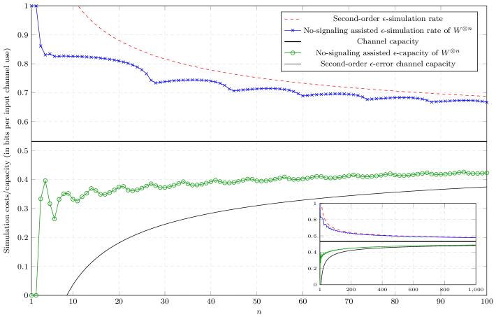
Figure 2: Consider i.i.d. copies of a binary symmetric channel $W$ with crossover probability $\delta=0.1$ and an error parameter $\epsilon=0.05$. The figure shows the second-order approximation of the common randomness assisted $\epsilon$-error simulation cost and the exact no-signaling assisted $\epsilon$-error simulation cost. This is contrasted with the corresponding quantities for channel coding, as discussed in [13], for example. The capacity of the channel is achieved for both tasks in the asymptotic limit.

I-A4 Asymptotic Expansions

For any $\epsilon\in(0,1)$ and $\delta>0$ small enough, we establish the following relationship between the task of channel simulation and the task of channel coding, i.e., (see Theorem 5)

$$\log{N_{1-\epsilon-\delta}^{\star}(W_{\mathsf{Y}|\mathsf{X}})}+\log{\delta}\leqslant\log{M_{\epsilon}^{\star}(W_{\mathsf{Y}|\mathsf{X}})}\leqslant\log{N_{1-\epsilon+\delta}^{\star}(W_{\mathsf{Y}|\mathsf{X}})}+\log{\frac{2}{\delta}}+\log{\log{\frac{4}{\delta^{2}}}}.$$ (8)

Using this relationship and the asymptotic expansions of the channel coding in the small deviation regime [19, 13, 14]

$$\log{N_{\epsilon}^{\star}(W_{\mathsf{Y}|\mathsf{X}}^{\otimes n})}=n\cdot C(W_{\mathsf{Y}|\mathsf{X}})+\sqrt{nV_{\epsilon}(W_{\mathsf{Y}|\mathsf{X}})}\cdot\Phi^{-1}(\epsilon)+O(\log{n}),$$ (9)

and in the moderate deviation regime (e.g., see [20]), i.e.,

$$\frac{1}{n}\log{N_{\epsilon_{n}}^{\star}(W_{\mathsf{Y}|\mathsf{X}}^{\otimes n})} =C(W_{\mathsf{Y}|\mathsf{X}})+\sqrt{2V_{\min}(W_{\mathsf{Y}|\mathsf{X}})}\cdot a_{n}+o(a_{n}),$$ (10)

$$\frac{1}{n}\log{N_{1-\epsilon_{n}}^{\star}(W_{\mathsf{Y}|\mathsf{X}}^{\otimes n})} =C(W_{\mathsf{Y}|\mathsf{X}})+\sqrt{2V_{\max}(W_{\mathsf{Y}|\mathsf{X}})}\cdot a_{n}+o(a_{n}),$$ (11)

where $\epsilon_{n}\coloneqq 2^{-na_{n}^{2}}$ and $\{a_{n}\}_{n=1}^{\infty}$ is some moderate sequence, we find asymptotic expansions for the channel simulation as direct results of Theorem 5 (see Corollary 8 and 9), i.e.,

$$\log{M_{\epsilon}^{\star}(W_{\mathsf{Y}|\mathsf{X}}^{\otimes n})} =n\cdot C(W_{\mathsf{Y}|\mathsf{X}})+\sqrt{nV_{1-\epsilon}(W_{\mathsf{Y}|\mathsf{X}})}\cdot\Phi^{-1}(1-\epsilon)+O(\log{n}),$$ (12)

$$\frac{1}{n}\log{M_{\epsilon_{n}}^{\star}(W_{\mathsf{Y}|\mathsf{X}}^{\otimes n})} =C(W_{\mathsf{Y}|\mathsf{X}})+\sqrt{2V_{\max}(W_{\mathsf{Y}|\mathsf{X}})}\cdot a_{n}+o(a_{n}),$$ (13)

$$\frac{1}{n}\log{M_{1-\epsilon_{n}}^{\star}(W_{\mathsf{Y}|\mathsf{X}}^{\otimes n})} =C(W_{\mathsf{Y}|\mathsf{X}})+\sqrt{2V_{\min}(W_{\mathsf{Y}|\mathsf{X}})}\cdot a_{n}+o(a_{n}).$$ (14)

Here, $C(\cdot)$ is the channel capacity, $\Phi(\cdot)$ is the cumulative distribution function of the standard normal distribution, and $V_{\epsilon}(W_{\mathsf{Y}|\mathsf{X}})$ is the $\epsilon$-channel dispersion known from channel coding (see, e.g., [13, 14]). These quantities are formally defined in Section III.

As a numerical example, we plot in Fig. 2 for the binary symmetric channel the meta converse and its asymptotic second-order expansion for both channel simulation and channel coding. Whereas the asymptotic first order rate is given by the same number for both tasks — the channel capacity — in the finite block-length regime there is a second-order gap

$$\left(\sqrt{nV_{1-\epsilon}(W_{\mathsf{Y}|\mathsf{X}})}+\sqrt{nV_{\epsilon}(W_{\mathsf{Y}|\mathsf{X}})}\right)\cdot\Phi^{-1}(\epsilon)$$ (15)

between the two values. As a consequence, even if we allow no-signaling assisted codes, the asymptotic first order reversibility of channel interconversion breaks down in second-order — unless the channel dispersion terms become zero. (Reversibility is discussed further at the end of this paper.) For example, the conversion between the ternary identity channel and the following ternary channel is reversible up to second order:

$$W_{\mathsf{Y}|\mathsf{X}}(y|x)=\begin{cases}\frac{1}{2}&\text{if }x\neq y\\ 0&\text{otherwise}\end{cases},$$ (16)

where $x,y\in\{0,1,2\}$.

I-A5 Broadcast Channel Simulation

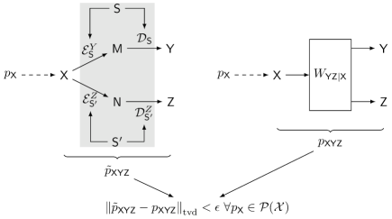
Figure 3: The task of simulating a bipartite broadcast channel with the help of common randomness between the sender and the two receivers, respectively, under the worst case error criteria given by the channel TVD.

We extend our results to network topologies and derive a channel simulation theorem for $K$-receiver broadcast channels. We provide a detailed discussion for the case when $K=2$. Namely, for the task of simulating $W_{\mathsf{YZ}|\mathsf{X}}$ under common randomness assistance, we characterize the asymptotic simulation rate region $\mathcal{R}^{\star}_{\epsilon}(W_{\mathsf{YZ}|\mathsf{X}})$, i.e., the closure of the set of all attainable rate pairs $(r_{1},r_{2})$ of $\epsilon$-simulation codes for $W_{\mathsf{YZ}|\mathsf{X}}^{\otimes n}$ for $n$ large enough, as (see Theorem 18)

$$\mathcal{R}^{\star}_{\epsilon}(W_{\mathsf{YZ}|\mathsf{X}})=\left\{(r_{1},r_{2})\in\mathbb{R}_{>0}^{2}\middle|r_{1}\geqslant C(W_{\mathsf{Y}|\mathsf{X}}),\,r_{2}\geqslant C(W_{\mathsf{Z}|\mathsf{X}}),\,r_{1}+r_{2}\geqslant\widetilde{C}(W_{\mathsf{YZ}|\mathsf{X}})\right\}.$$ (17)

Here, $C(W_{\mathsf{Y}|\mathsf{X}})$ denotes the channel capacity of the reduced channel $W_{\mathsf{Y}|\mathsf{X}}$ (same for $W_{\mathsf{Z}|\mathsf{X}}$), and $\widetilde{C}(W_{\mathsf{YZ}|\mathsf{X}})$ denotes the multi-partite mutual information of the broadcast channel $W_{\mathsf{YZ}|\mathsf{X}}$ defined as (see [21, 22]) (also see the general form (21) below)

$$\widetilde{C}(W_{\mathsf{YZ}|\mathsf{X}})\coloneqq\sup_{p_{\mathsf{X}}\in\mathcal{P}(\mathcal{X})}I(\mathsf{X}:\mathsf{Y}:\mathsf{Z})_{p_{\mathsf{X}}\cdot W_{\mathsf{YZ}|\mathsf{X}}}\quad\text{with}\quad I(\mathsf{X}:\mathsf{Y}:\mathsf{Z})\coloneqq H(\mathsf{X})+H(\mathsf{Y})+H(\mathsf{Z})-H(\mathsf{XYZ})$$ (18)

with $H(\mathsf{X})$ denoting the Shannon entropy of the marginal random variable $\mathsf{X}$. Our achievability bounds utilize a modified version of the bipartite convex split lemma from [23, 24], whereas the converse bound uses similar inequalities as in the point-to-point case.

Our characterizations give a direct operational interpretation to the multipartite mutual information of broadcast channels. We can also efficiently compute the rate region $\mathcal{R}^{\star}_{\epsilon}(W_{\mathsf{YZ}|\mathsf{X}})$, which is demonstrated in Fig. 5 by the means of iterative Blahut–Arimoto techniques. Fig. 5 further showcases that the sum rate constraint on $r_{1}+r_{2}$ in terms of the multipartite mutual information is in general necessary as

$$\widetilde{C}(W_{\mathsf{YZ}|\mathsf{X}})\geqslant C(W_{\mathsf{Y}|\mathsf{X}})+C(W_{\mathsf{Z}|\mathsf{X}})$$ (19)

typically becomes strict. We conclude that unlike the capacity region of broadcast channels — for which in general only non-matching inner and outer bounds are known [25] — our characterization of the simulation region is exact, has a single-letter form, and can be computed efficiently. Finally, by sub-additivity of the Shannon entropy we additionally have $\widetilde{C}(W_{\mathsf{YZ}|\mathsf{X}})\geqslant C(W_{\mathsf{YZ}|\mathsf{X}})$, which shows that employing a global decoder for channel simulation would lead to a less restrictive sum rate constraint. However, by the same argument of a global decoder, $C(W_{\mathsf{YZ}|\mathsf{X}})$ is also an outer bound on the channel capacity region of broadcast channels. Consequently we find that common randomness — or even no-signaling — assisted broadcast channel interconversion already becomes asymptotically irreversible in the first-order. This is in contrast to the point-to-point case, where we have seen that irreversibility only appears in the second-order.

For general $K$-receiver broadcast channels $W_{\mathsf{\mathbf{\mathsf{Y}}}_{1}^{K}|\mathsf{X}}$ from $\mathcal{X}$ to $\mathcal{Y}_{1}\times\cdots\times\mathcal{Y}_{K}$, we find the single-letter characterization (see Theorem 18)

$$\mathcal{R}^{\star}_{\epsilon}(W_{\mathbf{\mathsf{Y}}_{1}^{K}|\mathsf{X}})=\left\{(r_{1},\cdots,r_{n})\in\mathbb{R}_{>0}^{n}\,\middle|\,\sum_{i\in\mathcal{J}}r_{i}\geqslant\widetilde{C}(W_{\mathbf{\mathsf{Y}}_{\mathcal{J}}|\mathsf{X}})\quad\forall\mathcal{J}\subset\{1,\ldots,K\}\text{ with }\mathcal{J}\neq\emptyset\right\}$$ (20)

where for each $k=1,\ldots,K$,

$$\widetilde{C}(W_{\mathbf{\mathsf{Y}}_{1}^{k}|\mathsf{X}})\coloneqq\max_{p_{\mathsf{X}}\in\mathcal{P}(\mathcal{X})}I(\mathsf{X}:\mathsf{Y}_{1}:\ldots:\mathsf{Y}_{k})_{p_{\mathsf{X}}\cdot W_{\mathbf{\mathsf{Y}}_{1}^{k}|\mathsf{X}}},$$ (21)

and the multi-partite mutual information $I(\mathsf{X}:\mathsf{Y}_{1}:\ldots:\mathsf{Y}_{k})$ is defined in (146).

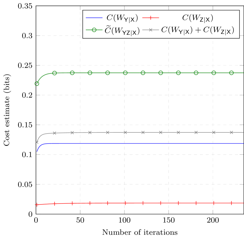
Figure 4: Convergence of the Blahut–Arimoto algorithm to the asymptotic simulation cost of simulating the broadcast channel $W_{\mathsf{YZ}|\mathsf{X}}=\mathrm{BSC}_{\mathsf{Z}|\mathsf{Y}}\circ\mathrm{BSC}_{\mathsf{Y}|\mathsf{X}}$, where $\mathrm{BSC}_{\mathsf{Z}|\mathsf{Y}}$ and $\mathrm{BSC}_{\mathsf{Y}|\mathsf{X}}$ are binary symmetric channels with crossover probability $\delta=0.3$. The iterative procedure stops when increments for all quantities are smaller than $10^{-9}$ bits.

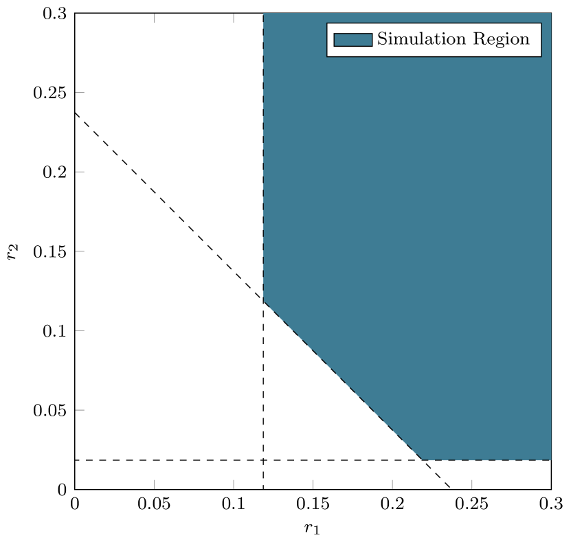
Figure 5: Asymptotic simulation region for the broadcast channel $W_{\mathsf{YZ}|\mathsf{X}}=\mathrm{BSC}_{\mathsf{Z}|\mathsf{Y}}\circ\mathrm{BSC}_{\mathsf{Y}|\mathsf{X}}$, where $\mathrm{BSC}_{\mathsf{Z}|\mathsf{Y}}$ and $\mathrm{BSC}_{\mathsf{Y}|\mathsf{X}}$ are binary symmetric channels with crossover probability $\delta=0.3$.

I-B Related Work

Various problems akin to channel interconversion (i.e., the general task of simulating one channel using another channel as a resource) and simulation have been studied in the literature and here we briefly comment on the relation to our work. We emphasize again that our black-box channel simulation requires simulation of the channel under arbitrary inputs as discussed in [2, 3], whereas most of the previous results focused on fixed input distributions. More comprehensive (partial) reviews of this field can be found in [10] and [26].

• The task of strong coordination [6] or channel synthesis [8, 9, 27] are closely related to channel simulation. Namely, for the strong coordination tasks one needs to realize a joint pmf $p_{\mathsf{XY}}$ across two parties, where one party receives $\mathsf{X}$ and the other party generates $\mathsf{Y}$ with the help of one-way communications from the former to the latter (with or without common randomness assistance). Our channel simulation can then be viewed as a universal strong coordination of $p_{\mathsf{Y}|\mathsf{X}}$ for all $p_{\mathsf{X}}$ with the help of unlimited common randomness.

• The complexity of correlation [18, 7] considers the expected amount of communication needed for common randomness-assisted strong coordination, where the expectation is taken over the input distribution. This is different from our analysis, which considers the worst-case communication for all possible inputs. Related to this, one-shot channel simulation using variable-length codes is considered in [28].

• The related channel resolvability problem was introduced in [5] for arbitrary inputs under a worst case error criteria. While the task is similar to channel simulation, it is a priori different and it would be interesting to research the approach of [5] for channel simulation.

• When only limited rates of common randomness are available, the reverse Shannon theorem channels quantifies the optimal communication rate for black-box channel simulation [2, 3]. In this more general setting, one has to distinguish between feedback channel simulation — when the receiver also gets a copy of the output of the channel — and non-feedback channel simulation as defined above. However, whenever a sufficient rate of common randomness is available, the optimal simulation rate for feedback and non-feedback channel simulation becomes the same [3]. We note that the fixed input case has been resolved earlier in [29] and extensions to interactive communication models are studied in [30]; we refer to the survey [10].

• Channel simulation restricted to fixed inputs has also been studied for various network topologies [8, 31] and extensions to channel interconversion are available as well (again for fixed inputs) [32, 33]. However, to the authors’ best knowledge, the characterization of black-box broadcast channel simulation with matching inner and outer bounds is complementary to all these previous works.

• One-shot bounds on the communication cost of quantum channel simulation have been discussed in [34, 35, 36]. However, restricting these bounds to classical channels leads to bounds that are not tight enough for deriving the finite block-length expansions we give here. No-signaling assisted quantum channel simulation is the topic of [12]. As such a quantum version of the $\epsilon$-smooth channel max-information was defined in [12, Def. 5] and our findings on the exact no-signaling achievability of the meta converse for channel simulation are also implied by [12, App. A]. However, the asymptotic expansion of the meta converse given in [12] is not second-order tight because it makes use of so-called de Finetti reductions [37], also termed universal states [38].

II One-Shot Upper and Lower Bounds for Random-Assisted Channel Simulation

In this section, we present a pair of achievability and converse bounds for the minimal attainable size of $\epsilon$-simulation codes for DMC $W_{\mathsf{Y}|\mathsf{X}}$. The achievability bound applies the method of rejection sampling and are inspired by [18]. The converse bound is a result of a series of relationships among information quantities.

II-A Achievability Bound

We use the method of rejection sampling for channel simulation. To simulate the output of a distribution $p_{\mathsf{Y}}\in\mathcal{P}(\mathcal{Y})$ using many copies of i.i.d. random variables $\mathsf{Y}_{1}\mathsf{Y}_{2}\ldots\sim q_{\mathsf{Y}}\times q_{\mathsf{Y}}\times\cdots$, rejection sampling applies the accept-reject algorithm for each $\mathsf{Y}_{i}$, i.e., $\mathsf{Y}_{i}$ is “accepted” and chosen as an output for simulating $p_{\mathsf{Y}}$ with probability $\lambda\cdot\frac{p_{\mathsf{Y}}(\mathsf{Y}_{i})}{q_{\mathsf{Y}}(\mathsf{Y}_{j})}$ (for some normalizer $\lambda>0$ such that this number is bounded by $1$). The procedure is stopped if $\mathsf{Y}_{i}$ is accepted, or moves onto $\mathsf{Y}_{i+1}$ otherwise. We formalize the details of this procedure and its analysis as the following lemma.

Lemma 1.

Let $p_{\mathsf{Y}},q_{\mathsf{Y}}\in\mathcal{P}(\mathcal{Y})$ such that $p\ll q$. Let $M\geqslant 1$ be an integer. Suppose $\mathsf{Y}_{1}$, $\mathsf{Y}_{2}$, …, $\mathsf{Y}_{M}$ are i.i.d. random variables where each $\mathsf{Y}_{j}$ is distributed according to $q_{\mathsf{Y}}$ for all $j=1,\ldots,M$. Let $\lambda\coloneqq\big{(}\max_{y\in\mathcal{Y}}\frac{p_{\mathsf{Y}}(y)}{q_{\mathsf{Y}}(y)}\big{)}^{-1}=2^{-D_{\max}\left(p_{\mathsf{Y}}\middle\|q_{\mathsf{Y}}\right)}$. We generate $\widetilde{\mathsf{Y}}$ conditioned on $\mathbf{\mathsf{Y}}_{1}^{M}$ using the following procedure:

1:$j\leftarrow 0$;

2:do

3:     $j\leftarrow j+1$;

4:     Generate random number $u\sim\mathcal{U}([0,1])$;

5:while $j<M$ and $u>\lambda\cdot\frac{p_{\mathsf{Y}}(\mathsf{Y}_{j})}{q_{\mathsf{Y}}(\mathsf{Y}_{j})}$

6:$\widetilde{\mathsf{Y}}\leftarrow\mathsf{Y}_{j}$

The procedure will create a random variable $\widetilde{\mathsf{Y}}$ jointly distributed with $\mathsf{Y}_{1},\ldots,\mathsf{Y}_{M}$. Let $\widetilde{p}_{\mathsf{Y}}$ denote the marginal distribution of $\widetilde{\mathsf{Y}}$. For any $\epsilon\in(0,1)$, if $M$ is large enough such that

$$\left(1-2^{-D_{\max}\left(p_{\mathsf{Y}}\middle\|q_{\mathsf{Y}}\right)}\right)^{M}\leqslant\epsilon,$$ (22)

then

$$\left\lVert p_{\mathsf{Y}}-\widetilde{p}_{\mathsf{Y}}\right\rVert_{\mathrm{tvd}}\leqslant\epsilon.$$ (23)

Proof.

Consider the procedure stated above. Let $\mathsf{A}$ be a binary random variable such that $\mathsf{A}=1$ if the program exited the loop (line 2–5) due to a violation of the second condition “$u>\lambda\cdot\frac{p_{\mathsf{Y}}(\mathsf{Y}_{j})}{q_{\mathsf{Y}}(\mathsf{Y}_{j})}$”. Otherwise, let $\mathsf{A}=0$. (In other words, $\mathsf{A}$ equals $1$ if one of the $\mathsf{Y}_{i}$’s was “accepted”, and equals $0$ otherwise.) By direct computation, we have

$$p_{\mathsf{A}}(0) =\sum_{y_{1},\ldots,y_{M}}\prod_{i=1}^{M}q_{\mathsf{Y}}(y_{i})\cdot\prod_{i=1}^{M}\left(1-\frac{p_{\mathsf{Y}}(y_{i})}{q_{\mathsf{Y}}(y_{i})}\cdot\left[\max_{y\in\mathcal{Y}}\frac{p_{\mathsf{Y}}(y)}{q_{\mathsf{Y}}(y)}\right]^{-1}\right)$$ (24)

$$=\sum_{y_{1},\ldots,y_{M}}\prod_{i=1}^{M}\left(q_{\mathsf{Y}}(y_{i})-p_{\mathsf{Y}}(y_{i})\cdot\left[\max_{y\in\mathcal{Y}}\frac{p_{\mathsf{Y}}(y)}{q_{\mathsf{Y}}(y)}\right]^{-1}\right)$$ (25)

$$=\left(1-\left(\max_{y\in\mathcal{Y}}\frac{p_{\mathsf{Y}}(y)}{q_{\mathsf{Y}}(y)}\right)^{-1}\right)^{M}=\left(1-2^{-D_{\max}\left(p_{\mathsf{Y}}\middle\|q_{\mathsf{Y}}\right)}\right)^{M}\leqslant\epsilon$$ (26)

where we used (22) (together with the definition of $D_{\max}$) for (26). On the other hand, for each $y\in\mathcal{Y}$,

$$p_{\widetilde{\mathsf{Y}}|\mathsf{A}}(y|1) =\frac{1}{p_{\mathsf{A}}(1)}\cdot\sum_{j=1}^{M}p_{\widetilde{Y}\mathsf{JA}}(y,j,1)=\frac{1}{p_{\mathsf{A}}(1)}\cdot\sum_{j=1}^{M}p_{\mathsf{Y}_{j}\mathsf{JA}}(y,j,1)=\frac{1}{p_{\mathsf{A}}(1)}\cdot\sum_{j=1}^{M}p_{\mathsf{JA}|\mathsf{Y}_{j}}(j,1|y)\cdot q_{\mathsf{Y}}(y)$$ (27)

$$=\frac{1}{1-p_{\mathsf{A}}(0)}\cdot\sum_{j=1}^{M}\sum_{y_{1}\ldots,y_{j\!-\!1}}\prod_{i=1}^{j-1}q_{\mathsf{Y}}(y_{i})\cdot\prod_{i=1}^{j-1}\left(1-\lambda\cdot\frac{p_{\mathsf{Y}}(y_{i})}{q_{\mathsf{Y}}(y_{i})}\right)\cdot\lambda\cdot\frac{p_{\mathsf{Y}}(y)}{q_{\mathsf{Y}}(y)}\cdot q_{\mathsf{Y}}(y)$$ (28)

$$=\frac{1}{1-\left(1-\lambda\right)^{M}}\cdot\sum_{j=1}^{M}\left(1-\lambda\right)^{j-1}\cdot\lambda\cdot p_{\mathsf{Y}}(y)=p_{\mathsf{Y}}(y)$$ (29)

where in (27), we summed over the probability of “acceptance” at $j$-th attempt while $\mathsf{Y}_{j}=y$. Thus,

$$\left\lVert p_{\mathsf{Y}}-\widetilde{p}_{\mathsf{Y}}\right\rVert_{\mathrm{tvd}} =\left\lVert p_{\mathsf{Y}}-(p_{\mathsf{A}}(1)\cdot p_{\mathsf{Y}}+p_{\mathsf{A}}(0)\cdot p^{\prime}_{\mathsf{Y}})\right\rVert_{\mathrm{tvd}}=\left\lVert p_{\mathsf{A}}(0)\cdot(p_{\mathsf{Y}}-p^{\prime}_{\mathsf{Y}})\right\rVert_{\mathrm{tvd}}\leqslant p_{\mathsf{A}}(0)\leqslant\epsilon$$ (30)

where $p^{\prime}_{\mathsf{Y}}$ is some pmf on $\mathcal{Y}$. ∎

Theorem 2 (One-Shot Achievability Bound).

Let $W_{\mathsf{Y}|\mathsf{X}}$ be a DMC from $\mathcal{X}$ to $\mathcal{Y}$, and let $\epsilon\in(0,1)$. It holds that

$$\log{M_{\epsilon}^{\star}(W_{\mathsf{Y}|\mathsf{X}})}\leqslant I_{\max}^{\epsilon-\delta}(W_{\mathsf{Y}|\mathsf{X}})+\log{\log{\frac{1}{\delta}}}.$$ (31)

for all $\delta\in(0,\epsilon]$.

Proof.

For arbitrary $q_{\mathsf{Y}}\in\mathcal{P}(\mathcal{Y})$ and DMC $\widetilde{W}_{\mathsf{Y}|\mathsf{X}}$ $(\epsilon-\delta)$-close to $W_{\mathsf{Y}|\mathsf{X}}$ in TVD, we describe the following protocol for simulating the channel $W_{\mathsf{Y}|\mathsf{X}}$ where $M$ is some positive integer to be determined later.

1. Let Alice and Bob share i.i.d. random variables $\mathsf{Y}_{1}$, $\mathsf{Y}_{2}$, …, $Y_{M}$, each distributed according to $q_{\mathsf{Y}}$.

2. Upon knowing $x\in\mathcal{X}$, Alice applies the accept-reject algorithm described in the previous lemma with parameters $M$, $p_{\mathsf{Y}}\leftarrow\widetilde{W}_{\mathsf{Y}|\mathsf{X}}(\cdot|x)$ and $q_{\mathsf{Y}}$, and send the index $j$ to Bob without loss (using a $M$-sized code).

3. Upon receiving $j$, Bob picks $\mathsf{Y}_{j}$ from the shared randomness and use it as the output of the simulated channel.

By Lemma 1, the channel created by the above protocol is $\delta$-close (in TVD) to $\widetilde{W}_{\mathsf{Y}|\mathsf{X}}$ if

$$\left(1-2^{-D_{\max}\left(\widetilde{W}_{\mathsf{Y}|\mathsf{X}}(\cdot|x)\middle\|q_{\mathsf{Y}}\right)}\right)^{M}\leqslant\delta$$ (32)

for all $x\in\mathcal{X}$. In this case, by the triangular inequality of the TVD for conditional probabilities, the simulated channel is $\epsilon$-close (in TVD) to $W_{\mathsf{Y}|\mathsf{X}}$. In other words, the $M$ chosen above is an upper bound to $M_{\epsilon}^{\star}(W_{\mathsf{Y}|\mathsf{X}})$. Since $q_{\mathsf{Y}}\in\mathcal{P}(\mathcal{Y})$ and $\widetilde{W}_{\mathsf{Y}|\mathsf{X}}$ (which is $(\epsilon-\delta)$-close to $W_{\mathsf{Y}|\mathsf{X}}$) in the above protocol can be chosen arbitrarily, by optimizing these two terms, we have

$$M_{\epsilon}^{\star}(W_{\mathsf{Y}|\mathsf{X}}) \leqslant\multiadjustlimits{\inf_{q_{\mathsf{Y}}\in\mathcal{P}(\mathcal{Y})},\inf_{\widetilde{W}_{\mathsf{Y}|\mathsf{X}}\in\mathcal{P}(\mathcal{Y}|\mathcal{X}):\left\lVert\widetilde{W}_{\mathsf{Y}|\mathsf{X}}-W_{\mathsf{Y}|\mathsf{X}}\right\rVert_{\mathrm{tvd}}\leqslant\epsilon-\delta},\sup_{x\in\mathcal{X}}}\frac{\log{\delta}}{\log\left(1-2^{-D_{\max}\left(\widetilde{W}_{\mathsf{Y}}|\mathsf{X}(\cdot|x)\middle\|q_{\mathsf{Y}}\right)}\right)}$$ (33)

$$=\log{\delta}\cdot\left\{\log{\left[1-2^{-\multiadjustlimits{\inf_{q_{\mathsf{Y}}\in\mathcal{P}(\mathcal{Y})},\inf_{\widetilde{W}_{\mathsf{Y}|\mathsf{X}}\in\mathcal{P}(\mathcal{Y}|\mathcal{X}):\left\lVert\widetilde{W}_{\mathsf{Y}|\mathsf{X}}-W_{\mathsf{Y}|\mathsf{X}}\right\rVert_{\mathrm{tvd}}\leqslant\epsilon-\delta},\max_{x\in\mathcal{X}}}D_{\max}\left(\widetilde{W}_{\mathsf{Y}}|\mathsf{X}(\cdot|x)\middle\|q_{\mathsf{Y}}\right)}\right]}\right\}^{-1}$$ (34)

$$=\log{\delta}\cdot\left(\log{\left(1-2^{-I_{\max}^{\epsilon-\delta}(W_{\mathsf{Y}|\mathsf{X}})}\right)}\right)^{-1}=\log{\frac{1}{\delta}}\cdot\left(-\log{\left(1-2^{-I_{\max}^{\epsilon-\delta}(W_{\mathsf{Y}|\mathsf{X}})}\right)}\right)^{-1}$$ (35)

$$\leqslant\log{\frac{1}{\delta}}\cdot 2^{I_{\max}^{\epsilon-\delta}(W_{\mathsf{Y}|\mathsf{X}})}$$ (36)

where we used the inequality $\log{(1-x)}\leqslant-x$ when $x\in[0,1)$ for (36). Finally, (31) is obtained by taking logarithm on both sides. ∎

II-B Converse Bound

Given a pair of discrete random variables $\mathsf{X}\mathsf{Y}$ with joint pmf $p_{\mathsf{XY}}\in\mathcal{P}(\mathcal{X}\times\mathcal{Y})$, the max-mutual information of $\mathsf{X}$ v.s.$\mathsf{Y}$ is defined as

$$I_{\max}(\mathsf{X}:\mathsf{Y})\coloneqq\inf_{q_{\mathsf{Y}}\in\mathcal{P}(\mathcal{Y})}D_{\max}\left(p_{\mathsf{XY}}\middle\|p_{\mathsf{X}}\times q_{\mathsf{Y}}\right)$$ (37)

where $p_{\mathsf{X}}$ is the marginal distribution of $\mathsf{X}$ induced from $p_{\mathsf{XY}}$.

Lemma 3.

Let $(\mathsf{X},\mathsf{Y},\mathsf{Z})$ be joint random variables distributed on $\mathcal{X}\times\mathcal{Y}\times\mathcal{Z}$. In particular, suppose the set $\mathcal{Z}$ is finite. Then,

$$I_{\max}(\mathsf{X}:\mathsf{YZ})\leqslant I_{\max}(\mathsf{X}:\mathsf{Y})+\log{\left\lvert\mathcal{Z}\right\rvert}.$$ (38)

This lemma can be derived as a special case of [39, Cor. A.14]. Here, we provide a direct and simpler proof.

Proof.

Let $q_{\mathsf{Y}}^{\star}$ denotes the optimal distribution on $\mathcal{Y}$ achieving the infimum in the definition of $I_{\max}(\mathsf{X}:\mathsf{Y})$. Then,

$$I_{\max}(\mathsf{X}:\mathsf{YZ}) =\inf_{q_{\mathsf{YZ}}\in\mathcal{P}(\mathcal{Y}\times\mathcal{Z})}D_{\max}\left(p_{\mathsf{XYZ}}\middle\|p_{\mathsf{X}}\times q_{\mathsf{YZ}}\right)$$ (39)

$$\leqslant D_{\max}\left(p_{\mathsf{XYZ}}\middle\|p_{\mathsf{X}}\times q_{\mathsf{Y}}^{\star}\times\frac{1}{\left\lvert\mathcal{Z}\right\rvert}\right)$$ (40)

$$=\log{\left(\left\lvert\mathcal{Z}\right\rvert\cdot\sup_{x,y,z}\frac{p_{\mathsf{XY}}(x,y)\cdot p_{\mathsf{Z}|\mathsf{XY}}(z|x,y)}{p_{\mathsf{X}}\cdot q_{\mathsf{Y}}^{\star}(y)}\right)}$$ (41)

$$\leqslant\log{\left(\sup_{x,y}\frac{p_{\mathsf{XY}}(x,y)}{p_{\mathsf{X}}\cdot q_{\mathsf{Y}}^{\star}(y)}\right)}+\log{\left\lvert\mathcal{Z}\right\rvert}$$ (42)

$$=I_{\max}(\mathsf{X}:\mathsf{Y})+\log{\left\lvert\mathcal{Z}\right\rvert}.\qed$$ (43)

Theorem 4 (One-Shot Converse Bound).

Let $W_{\mathsf{Y}|\mathsf{X}}$ be a DMC from $\mathcal{X}$ to $\mathcal{Y}$, and let $\epsilon\in(0,1)$. Then

$$\log{M^{\star}_{\epsilon}(W_{\mathsf{Y}|\mathsf{X}})}\geqslant I_{\max}^{\epsilon}(W_{\mathsf{Y}|\mathsf{X}})$$ (44)

and, since $M^{\star}_{\epsilon}(W_{\mathsf{Y}|\mathsf{X}})$ is an integer, it must also satisfy $M^{\star}_{\epsilon}(W_{\mathsf{Y}|\mathsf{X}})\geqslant\left\lceil 2^{I_{\max}^{\epsilon}(W_{\mathsf{Y}|\mathsf{X}})}\right\rceil$.

Proof.

Suppose there exists some size-$M$ $\epsilon$-simulation code for $W_{\mathsf{Y}|\mathsf{X}}$. Let random variable $\mathsf{S}$ denote the shared randomness, and $\mathsf{M}$ denote the code-word transmitted (see Fig. 1). Then, for any input source $\mathsf{X}\sim p_{\mathsf{X}}$, we have a Markov chain $\mathsf{X}-\mathsf{MS}-\mathsf{Y}$ where

• The distribution of $\mathsf{XY}$, denoted by $\widetilde{p}_{\mathsf{XY}}$, is $\epsilon$-close (in TVD) to $p_{\mathsf{XY}}\coloneqq p_{\mathsf{X}}\cdot W_{\mathsf{Y}|\mathsf{X}}$.

• The marginal distribution $\widetilde{p}_{\mathsf{X}}=\sum_{y}\widetilde{p}_{\mathsf{XY}}(\cdot,y)=p_{\mathsf{X}}$.

• $\mathsf{M}$ is distributed over $\{1,\ldots,M\}$.

Pick $p_{\mathsf{X}}$ to be some pmf with full support. We have following series of inequalities.

1. By Lemma 3, we have

   $$\log{M}=I_{\max}(\mathsf{X}:\mathsf{S})+\log{M}\geqslant I_{\max}(\mathsf{X}:\mathsf{MS}).$$ (45)

2. By the data-processing inequality of $I_{\max}$, we have

   $$I_{\max}(\mathsf{X}:\mathsf{MS})\geqslant I_{\max}(\mathsf{X}:\mathsf{Y})$$ (46)

3. By the definition of $I_{\max}$ and the fact that $\widetilde{p}_{\mathsf{X}}=p_{\mathsf{X}}$, we have

   $$I_{\max}(\mathsf{X}:\mathsf{Y}) =\inf_{q_{\mathsf{Y}}}D_{\max}\left(\widetilde{p}_{\mathsf{XY}}\middle\|p_{\mathsf{X}}\times q_{\mathsf{Y}}\right)$$ (47)

   $$=\adjustlimits{\inf}_{q_{\mathsf{Y}}}{\max}_{x}D_{\max}\left(\widetilde{p}_{\mathsf{Y}|\mathsf{X}}(\cdot|x)\middle\|q_{\mathsf{Y}}\right)$$ (48)

   $$\geqslant\multiadjustlimits{\inf_{q_{\mathsf{Y}}},\inf_{\widetilde{W}_{\mathsf{Y}|\mathsf{X}}:\left\lVert\widetilde{W}_{\mathsf{Y}|\mathsf{X}}-W_{\mathsf{Y}|\mathsf{X}}\right\rVert_{\mathrm{tvd}}\leqslant\epsilon},\max_{x}}D_{\max}\left(\widetilde{W}_{\mathsf{Y}|\mathsf{X}}(\cdot|x)\middle\|q_{\mathsf{Y}}\right)=I_{\max}^{\epsilon}(W_{\mathsf{Y}|\mathsf{X}})$$ (49)

   where the last inequality holds since $\widetilde{p}_{\mathsf{Y}|\mathsf{X}}$, i.e., the simulated channel as the result of the size-$M$ simulation code, is $\epsilon$-close to $W_{\mathsf{Y}|\mathsf{X}}$ in TVD.

Combining the above, we have shown $\log{M}\geqslant I_{\max}^{\epsilon}(W_{\mathsf{Y}|\mathsf{X}})$ for any admissible $M$. Since $M^{\star}_{\epsilon}(W_{\mathsf{Y}|\mathsf{X}})$ is the infimum of all such $M$’s, the inequality must also hold with $M^{\star}_{\epsilon}(W_{\mathsf{Y}|\mathsf{X}})$. ∎

III Asymptotic Analysis in Small Deviation and Moderate Deviation Regimes

In this section, we consider the problem of simulating $n$ copies of $W_{\mathsf{Y}|\mathsf{X}}$, i.e., $W_{\mathsf{Y}|\mathsf{X}}^{\otimes n}$, under both fixed TVD-tolerance $\epsilon\in(0,1)$ and sub-exponentially decaying TVD-tolerance,

$$\epsilon_{n}=2^{-na_{n}^{2}},$$ (50)

where $\{a_{n}\}_{n\in\mathbb{N}}$ is some moderate sequence, i.e., a sequence of positive numbers such that $a_{n}\to 0$ but $na_{n}^{2}\to+\infty$ as $n\to\infty$. The former is known as the small deviation or fixed error regime whereas the latter is known as the moderate deviation regime. We are interested in the asymptotic expansion of $\log{M_{\epsilon_{n}}^{\star}(W_{\mathsf{Y}|\mathsf{X}}^{\otimes n})}$ (as a function of $n$) in both cases.

First, we establish the following relationship between the minimal channel simulation cost and the maximal channel coding size (under the average error).

Theorem 5.

Let $W_{\mathsf{Y}|\mathsf{X}}$ be a DMC and $\epsilon\in(0,1)$. For each $n\in\mathbb{N}$. Let $N_{\epsilon}^{\star}(W_{\mathsf{Y}|\mathsf{X}})$ denote the largest integer $N$ such that there exists a size-$N$ code with transmission error probability (over $W_{\mathsf{Y}|\mathsf{X}}$) at most $\epsilon$ given equiprobable codewords. It holds that

$$\log{N_{1-\epsilon-\delta}(W_{\mathsf{Y}|\mathsf{X}})}+\log{\delta}\leqslant\log{M_{\epsilon}^{\star}(W_{\mathsf{Y}|\mathsf{X}})}\leqslant\log{N_{1-\epsilon+\delta}(W_{\mathsf{Y}|\mathsf{X}})}+\log{\frac{2}{\delta}}+\log{\log{\frac{4}{\delta^{2}}}}$$ (51)

for any $\delta\in(0,\min\{\epsilon,1-\epsilon\})$.

Proof.

To prove the first inequality, we have

$$\log{M_{\epsilon}^{\star}(W_{\mathsf{Y}|\mathsf{X}})} \geqslant I_{\max}^{\epsilon}(W_{\mathsf{Y}|\mathsf{X}})=\multiadjustlimits{\inf_{\widetilde{W}_{\mathsf{Y}|\mathsf{X}}:\left\lVert\widetilde{W}_{\mathsf{Y}|\mathsf{X}}-W_{\mathsf{Y}|\mathsf{X}}\right\rVert_{\mathrm{tvd}}\leqslant\epsilon},\sup_{p_{\mathsf{X}}},\inf_{q_{\mathsf{Y}}}}D_{\max}\left(p_{\mathsf{X}}\cdot\widetilde{W}_{\mathsf{Y}|\mathsf{X}}\middle\|p_{\mathsf{X}}\times q_{\mathsf{Y}}\right)$$ (52)

$$\geqslant\multiadjustlimits{\sup_{p_{\mathsf{X}}\in\mathcal{P}(\mathcal{X})},\inf_{q_{\mathsf{Y}}\in\mathcal{P}(\mathcal{Y})},\inf_{\widetilde{W}_{\mathsf{Y}|\mathsf{X}}:\left\lVert p_{\mathsf{X}}\cdot\widetilde{W}_{\mathsf{Y}|\mathsf{X}}-p_{\mathsf{X}}\cdot W_{\mathsf{Y}|\mathsf{X}}\right\rVert_{\mathrm{tvd}}\leqslant\epsilon}}D_{\max}\left(p_{\mathsf{X}}\cdot\widetilde{W}_{\mathsf{Y}|\mathsf{X}}\middle\|p_{\mathsf{X}}\times q_{\mathsf{Y}}\right)$$ (53)

$$\geqslant\multiadjustlimits{\sup_{p_{\mathsf{X}}\in\mathcal{P}(\mathcal{X})},\inf_{q_{\mathsf{Y}}\in\mathcal{P}(\mathcal{Y})},\inf_{\widetilde{p}_{\mathsf{XY}}\in\mathcal{P}(\mathcal{X}\times\mathcal{Y}):\left\lVert\widetilde{p}_{\mathsf{XY}}-p_{\mathsf{XY}}\right\rVert_{\mathrm{tvd}}\leqslant\epsilon}}D_{\max}\left(p_{\mathsf{X}}\cdot\widetilde{W}_{\mathsf{Y}|\mathsf{X}}\middle\|p_{\mathsf{X}}\times q_{\mathsf{Y}}\right)$$ (54)

$$\geqslant\adjustlimits{\sup}_{p_{\mathsf{X}}\in\mathcal{P}(\mathcal{X})}{\inf}_{q_{\mathsf{Y}}\in\mathcal{P}(\mathcal{Y})}\log{\frac{1}{\beta_{1-\epsilon-\delta}^{\star}\left(p_{\mathsf{X}}\cdot W_{\mathsf{Y}|\mathsf{X}}\middle\|p_{\mathsf{X}}\cdot q_{\mathsf{Y}}\right)}}+\log{\delta} \forall\delta\in(0,1-\epsilon)$$ (55)

$$\geqslant\log{N_{1-\epsilon-\delta}(W_{\mathsf{Y}|\mathsf{X}})}+\log{\delta}$$ (56)

where, in (53), we swap $\inf_{\widetilde{W}_{\mathsf{Y}|\mathsf{X}}}$ inside and relax the domain for $\widetilde{W}_{\mathsf{Y}|\mathsf{X}}$; in (54), we relax the domain of the infimum; in (55), we use Lemma 6 below; and in (56), we use Theorem 27 from [13], and substitute $\delta_{1}=\delta_{2}\leftarrow\delta/2$.

To prove the second inequality, we have

$$\log{M_{\epsilon}^{\star}(W_{\mathsf{Y}|\mathsf{X}})} \leqslant I_{\max}^{\epsilon-\delta_{1}}(W_{\mathsf{Y}|\mathsf{X}})+\log{\log{\frac{1}{\delta_{1}}}} \forall\delta_{1}\in(0,\epsilon_{1})$$ (57)

$$=\multiadjustlimits{\inf_{q_{\mathsf{Y}}\in\mathcal{P}(\mathcal{Y})},\inf_{\widetilde{W}_{\mathsf{Y}|\mathsf{X}}:\left\lVert\widetilde{W}_{\mathsf{Y}|\mathsf{X}}-W_{\mathsf{Y}|\mathsf{X}}\right\rVert_{\mathrm{tvd}}\leqslant\epsilon-\delta_{1}},\max_{x\in\mathcal{X}}}D_{\max}\left(\widetilde{W}_{\mathsf{Y}|\mathsf{X}}(\cdot|x)\middle\|q_{\mathsf{Y}}\right)+\log{\log{\frac{1}{\delta_{1}}}}$$ (58)

$$\leqslant\multiadjustlimits{\inf_{q_{\mathsf{Y}}\in\mathcal{P}(\mathcal{Y})},\sup_{p_{\mathsf{X}}\in\mathcal{P}(\mathcal{X})}}D_{s+}^{\epsilon-\delta_{1}}\left(p_{\mathsf{X}}\cdot W_{\mathsf{Y}|\mathsf{X}}\middle\|p_{\mathsf{X}}\times q_{\mathsf{Y}}\right)+\log{\log{\frac{1}{\delta_{1}^{2}}}}$$ (59)

$$\leqslant\multiadjustlimits{\inf_{q_{\mathsf{Y}}\in\mathcal{P}(\mathcal{Y})},\sup_{p_{\mathsf{X}}\in\mathcal{P}(\mathcal{X})}}\log{\frac{1}{\beta_{1-\epsilon+\delta_{1}}^{\star}\left(p_{\mathsf{X}}\cdot W_{\mathsf{Y}|\mathsf{X}}\middle\|p_{\mathsf{X}}\times q_{\mathsf{Y}}\right)}}+\log{\log{\frac{1}{\delta_{1}^{2}}}}$$ (60)

$$=\adjustlimits{\sup}_{p_{\mathsf{X}}\in\mathcal{P}(\mathcal{X})}{\inf}_{q_{\mathsf{Y}}\in\mathcal{P}(\mathcal{Y})}\log{\frac{1}{\beta_{1-\epsilon+\delta_{1}}^{\star}\left(p_{\mathsf{X}}\cdot W_{\mathsf{Y}|\mathsf{X}}\middle\|p_{\mathsf{X}}\times q_{\mathsf{Y}}\right)}}+\log{\log{\frac{1}{\delta_{1}^{2}}}}$$ (61)

$$\leqslant\sup_{p_{\mathsf{X}}\in\mathcal{P}(\mathcal{X})}\log{\frac{1}{\beta_{1-\epsilon+\delta_{1}}^{\star}\left(p_{\mathsf{X}}\cdot W_{\mathsf{Y}|\mathsf{X}}\middle\|p_{\mathsf{X}}\times p_{\mathsf{Y}}\right)}}+\log{\log{\frac{1}{\delta_{1}^{2}}}}$$ (62)

$$\leqslant\log{N^{\star}_{1-\epsilon+\delta_{1}+\delta_{2}}}(W_{\mathsf{Y}|\mathsf{X}})+\log{\frac{1}{\delta_{2}}}+\log{\log{\frac{1}{\delta_{1}^{2}}}} \forall\delta_{2}\in(0,\epsilon-\delta_{1})$$ (63)

$$=\log{N^{\star}_{1-\epsilon+\delta}}(W_{\mathsf{Y}|\mathsf{X}})+\log{\frac{2}{\delta}}+\log{\log{\frac{4}{\delta^{2}}}} \forall\delta\in(0,\epsilon)$$ (64)

where, in (59), we use Lemma 7 below (also see the definition of $D_{s+}$ in (70)); in (60), we use Lemma 12 from [40]; in (61), we use the saddle point property of $\beta_{\epsilon}^{\star}(p_{\mathsf{X}}\cdot W_{\mathsf{Y}|\mathsf{X}}\|p_{\mathsf{X}}\times q_{\mathsf{Y}})$ [41]; in (63), we use the achievability bound

$$N_{\epsilon+\delta}^{\star}(W_{\mathsf{Y}|\mathsf{X}})\geqslant\sup_{p_{\mathsf{X}}\in\mathcal{P}(\mathcal{X})}\frac{\delta}{\beta^{\star}_{\epsilon}(p_{\mathsf{X}}\cdot W_{\mathsf{Y}|\mathsf{X}},p_{\mathsf{X}}\times p_{\mathsf{Y}})}\quad\forall\delta\in(0,1-\epsilon);$$ (65)

and in (64), we substitute $\delta_{1}=\delta_{2}\leftarrow\delta/2$. ∎

Lemma 6.

Let $p$ and $q$ be two pmfs on a same alphabet. It holds for all $\epsilon\in(0,1)$, $\delta\in(0,1-\epsilon)$ that

$$D_{\max}^{\epsilon}\left(p\middle\|q\right)\geqslant\log{\frac{1}{\beta_{1-\epsilon-\delta}\left(p\middle\|q\right)}}+\log{\delta}.$$ (66)

Proof.

Suppose $p$ and $q$ are pmfs on $\mathcal{X}$. Let $\widetilde{p}\in\mathcal{P}(\mathcal{X})$ be an optimizer for $D_{\max}^{\epsilon}\left(p\middle\|q\right)$, i.e., $\left\lVert\widetilde{p}-p\right\rVert_{\mathrm{tvd}}\leqslant\epsilon$ and $\widetilde{p}(x)\leqslant 2^{D_{\max}^{\epsilon}\left(p\middle\|q\right)}\cdot q(x)$ for all $x\in\mathcal{X}$. Let $\mathcal{A}\in\mathcal{X}$ be an optimizing subset for $\beta_{1-\epsilon-\delta}\left(p\middle\|q\right)$, i.e., $p(\mathcal{A})\geqslant\epsilon+\delta$ and $q(\mathcal{A})=\beta_{1-\epsilon-\delta}\left(p\middle\|q\right)$. Combining these two facts, we have

$$\epsilon\geqslant\left\lVert\widetilde{p}-p\right\rVert_{\mathrm{tvd}}\geqslant p(\mathcal{A})-\widetilde{p}(\mathcal{A})\geqslant\epsilon+\delta-2^{D_{\max}^{\epsilon}\left(p\middle\|q\right)}\cdot q(\mathcal{A})=\epsilon+\delta-2^{D_{\max}^{\epsilon}\left(p\middle\|q\right)}\cdot\beta_{1-\epsilon-\delta}\left(p\middle\|q\right).$$ (67)

Rearranging the terms, we get

$$2^{D_{\max}^{\epsilon}\left(p\middle\|q\right)}\cdot\beta_{1-\epsilon-\delta}\left(p\middle\|q\right)\geqslant\delta.$$ (68)

Eq. (66) can be proven by taking logarithm of the above inequality on both sides and shuffle the term $\log{\beta_{1-\epsilon-\delta}\left(p\middle\|q\right)}$ to the other side. ∎

Lemma 7.

Let $W_{\mathsf{Y}|\mathsf{X}}$ be a DMC from $\mathcal{X}$ to $\mathcal{Y}$ where both $\mathcal{X}$ and $\mathcal{Y}$ are some finite sets. It holds for all $\epsilon\in(0,1)$ that

$$\sup_{p_{\mathsf{X}}\in\mathcal{P}(\mathcal{X})}D_{s+}^{\epsilon}\left(p_{\mathsf{X}}\cdot W_{\mathsf{Y}|\mathsf{X}}\middle\|p_{\mathsf{X}}\times q_{\mathsf{Y}}\right)+1\geqslant\adjustlimits{\inf}_{\widetilde{W}_{\mathsf{Y}|\mathsf{X}}:\left\lVert\widetilde{W}_{\mathsf{Y}|\mathsf{X}}-W_{\mathsf{Y}|\mathsf{X}}\right\rVert_{\mathrm{tvd}}\leqslant\epsilon}{\max}_{x\in\mathcal{X}}D_{\max}\left(\widetilde{W}_{\mathsf{Y}|\mathsf{X}}(\cdot|x)\middle\|q_{\mathsf{Y}}\right)$$ (69)

for any $q_{\mathsf{Y}}\in\mathcal{P}(\mathcal{Y})$. Here, for any two pmfs $p$ and $q$ on a same alphabet, the spectrum divergence between $p$ and $q$ is defined as

$$D_{s+}^{\epsilon}\left(p\middle\|q\right)\coloneqq\inf\left\{a\geqslant 0\middle|\Pr_{\mathsf{X}\sim p}\left[\log{\frac{p(\mathsf{X})}{q(\mathsf{X})}}>a\right]<\epsilon\right\}.$$ (70)

The following proof is partially inspired by some of the arguments in the proof of [11, Theorem 9].

Proof.

If the LHS $=\infty$, the inequality holds trivially. Assuming otherwise, let $a\coloneqq\sup_{p_{\mathsf{X}}\in\mathcal{P}(\mathcal{X})}D_{s+}^{\epsilon}\left(p_{\mathsf{X}}\cdot W_{\mathsf{Y}|\mathsf{X}}\middle\|p_{\mathsf{X}}\times q_{\mathsf{Y}}\right)$. By the definition of $D_{s+}^{\epsilon}$ and the right semi-continuity of $a\mapsto\Pr_{\mathsf{XY}\sim p_{\mathsf{X}}\cdot W_{\mathsf{Y}|\mathsf{X}}}[\log{\frac{W_{\mathsf{Y}|\mathsf{X}}(\mathsf{Y}|\mathsf{X})}{q_{\mathsf{Y}}(\mathsf{Y})}}>a]$, we have, for all $p_{\mathsf{X}}\in\mathcal{P}(\mathcal{X})$,

$$\epsilon\geqslant\Pr\nolimits_{\mathsf{XY}\sim p_{\mathsf{X}}\cdot W_{\mathsf{Y}|\mathsf{X}}}\left[\log{\frac{W_{\mathsf{Y}|\mathsf{X}}(\mathsf{Y}|\mathsf{X})}{q_{\mathsf{Y}}(\mathsf{Y})}}>a\right]=\sum_{x\in\mathcal{X}}p_{\mathsf{X}}(x)\cdot\underbrace{\sum_{y\in\mathcal{Y}}W_{\mathsf{Y}|\mathsf{X}}(y|x)\cdot\mathbbm{1}\left\{\log{\frac{W_{\mathsf{Y}|\mathsf{X}}(y|x)}{q_{\mathsf{Y}}(y)}}>a\right\}}_{\eqqcolon\epsilon_{x}},$$ (71)

which forces $\epsilon_{x}\leqslant\epsilon$ for all $x\in\mathcal{X}$. For each $x\in\mathcal{X}$, let $\mathcal{A}_{x}$ denote the following subset of $\mathcal{Y}$

$$\mathcal{A}_{x}\coloneqq\left\{y\in\mathcal{Y}:\log{\frac{W_{\mathsf{Y}|\mathsf{X}}(y|x)}{q_{\mathsf{Y}}(y)}}\leqslant a\right\}.$$ (72)

We construct a DMC $\hat{W}_{\mathsf{Y}|\mathsf{X}}$ as

$$\hat{W}_{\mathsf{Y}|\mathsf{X}}(y|x)\coloneqq\begin{cases}W_{\mathsf{Y}|\mathsf{X}}(y|x)+\epsilon_{x}\cdot q_{\mathsf{Y}}(y)&\text{if }y\in\mathcal{A}_{x},\\ \epsilon_{x}\cdot q_{\mathsf{Y}}(y)&\text{otherwise}.\end{cases}$$ (73)

The construction ensures $\hat{W}_{\mathsf{Y}|\mathsf{X}}(\cdot|x)\leqslant(2^{a}+\epsilon_{x})\cdot q_{\mathsf{Y}}\leqslant(2^{a}+\epsilon)\cdot q_{\mathsf{Y}}$ for all $x$, and thus we have

$$\max_{x\in\mathcal{X}}D_{\max}\left(\hat{W}_{\mathsf{Y}|\mathsf{X}}(\cdot|x)\middle\|q_{\mathsf{Y}}\right)\leqslant\log\left(2^{a}+\epsilon\right)\leqslant a+1=\sup_{p_{\mathsf{X}}\in\mathcal{P}(\mathcal{X})}D_{s+}^{\epsilon}\left(p_{\mathsf{X}}\cdot W_{\mathsf{Y}|\mathsf{X}}\middle\|p_{\mathsf{X}}\times q_{\mathsf{Y}}\right)+1.$$ (74)

On the other hand we can show $\left\lVert\hat{W}_{\mathsf{Y}|\mathsf{X}}-W_{\mathsf{Y}|\mathsf{X}}\right\rVert_{\mathrm{tvd}}\leqslant\epsilon$ as

$$\max_{x\in\mathcal{X}}\left\lVert\hat{W}_{\mathsf{Y}|\mathsf{X}}(\cdot|x)-W_{\mathsf{Y}|\mathsf{X}}(\cdot|x)\right\rVert_{\mathrm{tvd}} =\max_{x\in\mathcal{X}}\frac{1}{2}\sum_{y\in\mathcal{A}_{x}^{C}}\left\lvert\epsilon_{x}q_{\mathsf{Y}}(y)-W_{\mathsf{Y}|\mathsf{X}}(y|x)\right\rvert+\sum_{y\in\mathcal{A}_{x}}\epsilon_{x}q_{\mathsf{Y}}(y)$$ (75)

$$\leqslant\max_{x}\frac{1}{2}\left(\epsilon_{x}+\sum_{y\in\mathcal{Y}}W_{\mathsf{Y}|\mathsf{X}}(y|x)\cdot\mathbbm{1}\left\{\log{\frac{W_{\mathsf{Y}|\mathsf{X}}(y|x)}{q_{\mathsf{Y}}(y)}}>a\right\}\right)$$ (76)

$$=\max_{x}\epsilon_{x}\leqslant\epsilon.$$ (77)

Therefore,

$$\max_{x\in\mathcal{X}}D_{\max}\left(\hat{W}_{\mathsf{Y}|\mathsf{X}}(\cdot|x)\middle\|q_{\mathsf{Y}}\right)\geqslant\inf_{\widetilde{W}_{\mathsf{Y}|\mathsf{X}}:\left\lVert\widetilde{W}_{\mathsf{Y}|\mathsf{X}}-W_{\mathsf{Y}|\mathsf{X}}\right\rVert_{\mathrm{tvd}}}\max_{x\in\mathcal{X}}D_{\max}\left(\widetilde{W}_{\mathsf{Y}|\mathsf{X}}(\cdot|x)\middle\|q_{\mathsf{Y}}\right)$$ (78)

Finally, (69) is proven by combining (74) and (78). ∎

Theorem 5 provides a direct relationship between minimal cost $M_{\epsilon}^{\star}(W_{\mathsf{Y}|\mathsf{X}})$ of the $\epsilon$-tolerance channel simulation and the maximal code size $N_{1-\epsilon}^{\star}(W_{\mathsf{Y}|\mathsf{X}})$ for $(1-\epsilon)$-error channel coding. Note that the asymptotic second-order expansion for the channel coding has been well studied [19, 13, 14], i.e.,

$$\log{N_{\epsilon}^{\star}(W_{\mathsf{Y}|\mathsf{X}}^{\otimes n})}=n\cdot C(W_{\mathsf{Y}|\mathsf{X}})+\sqrt{nV_{\epsilon}(W_{\mathsf{Y}|\mathsf{X}})}\cdot\Phi^{-1}(\epsilon)+O(\log{n}),$$ (79)

where

$$C(W_{\mathsf{Y}|\mathsf{X}}) \coloneqq\max_{p_{\mathsf{X}}\in\mathcal{P}(\mathcal{X})}I(\mathsf{X}:\mathsf{Y})_{p_{\mathsf{X}\cdot W_{\mathsf{Y}|\mathsf{X}}}}$$ (80)

$$V_{\epsilon}(W_{\mathsf{Y}|\mathsf{X}}) \coloneqq\begin{cases}V_{\min}(W_{\mathsf{Y}|\mathsf{X}})\coloneqq\min_{p_{\mathsf{X}}\in\Pi}V(p_{\mathsf{X}})&\text{if }\epsilon<\frac{1}{2}\\ V_{\max}(W_{\mathsf{Y}|\mathsf{X}})\coloneqq\max_{p_{\mathsf{X}}\in\Pi}V(p_{\mathsf{X}})&\text{if }\epsilon\geqslant\frac{1}{2}\end{cases}$$ (81)

$$\Pi \coloneqq\left\{p_{\mathsf{X}}\in\mathcal{P}(\mathcal{X})\middle|\,I(\mathsf{X}:\mathsf{Y})_{p_{\mathsf{X}}\cdot W_{\mathsf{Y}|\mathsf{X}}}=C(W_{\mathsf{Y}|\mathsf{X}})\right\},$$ (82)

$$V(p_{\mathsf{X}}) \coloneqq V\left(p_{\mathsf{X}}\cdot W_{\mathsf{Y}|\mathsf{X}}\middle\|p_{\mathsf{X}}\times\sum_{x}p_{\mathsf{X}}(x)\cdot W_{\mathsf{Y}|\mathsf{X}}(\cdot|x)\right)$$ (83)

$$V(p\|q) \coloneqq\mathrm{Var}\left(\log{\frac{p(\mathsf{X})}{q(\mathsf{X})}}\right)=\sum_{x\in\mathcal{X}}p(x)\cdot\left(\log{\frac{p(x)}{q(x)}}-D(p\|q)\right)^{2}\text{assuming $p\ll q$}.$$ (84)

Combing the above expansion with Theorem 5, we have the following corollary.

Corollary 8.

Let $W_{\mathsf{Y}|\mathsf{X}}$ be a DMC and $\epsilon\in(0,1)$. For each $n\in\mathbb{N}$, it holds that

$$\log{M_{\epsilon}^{\star}(W_{\mathsf{Y}|\mathsf{X}}^{\otimes n})}=n\cdot C(W_{\mathsf{Y}|\mathsf{X}})+\sqrt{nV_{1-\epsilon}(W_{\mathsf{Y}|\mathsf{X}})}\cdot\Phi^{-1}(\epsilon)+O(\log{n}).$$ (85)

Proof.

This is a direct result of (51) with $\delta\leftarrow\frac{1}{\sqrt{n}}$, and (79), namely

$$\log{M_{\epsilon}^{\star}(W_{\mathsf{Y}|\mathsf{X}}^{\otimes n})} \leqslant n\cdot C(W_{\mathsf{Y}|\mathsf{X}})+\sqrt{n\cdot V_{1-\epsilon+\frac{1}{\sqrt{n}}}(W_{\mathsf{Y}|\mathsf{X}})}\cdot\Phi^{-1}(1-\epsilon+\frac{1}{\sqrt{n}})+O(\log{n}),$$ (86)

$$\log{M_{\epsilon}^{\star}(W_{\mathsf{Y}|\mathsf{X}}^{\otimes n})} \geqslant n\cdot C(W_{\mathsf{Y}|\mathsf{X}})+\sqrt{n\cdot V_{1-\epsilon-\frac{1}{\sqrt{n}}}(W_{\mathsf{Y}|\mathsf{X}})}\cdot\Phi^{-1}(1-\epsilon-\frac{1}{\sqrt{n}})+O(\log{n}).$$ (87)

Note that, for $n$ large enough

$$\left\lvert\Phi^{-1}(1-\epsilon\pm\frac{1}{\sqrt{n}})-\Phi^{-1}(1-\epsilon)\right\rvert\leqslant\frac{1}{\sqrt{n}}\cdot\max_{t\in[\frac{1-\epsilon}{2},1-\frac{\epsilon}{2}]}\frac{\operatorname{d}}{\operatorname{d}t}\Phi^{-1}(t)\leqslant\frac{1}{\sqrt{n}}\cdot\text{constant}.$$ (88)

Thus, we have

$$\log{M_{\epsilon}^{\star}(W_{\mathsf{Y}|\mathsf{X}}^{\otimes n})} \leqslant n\cdot C(W_{\mathsf{Y}|\mathsf{X}})+\sqrt{n\cdot V_{1-\epsilon+\frac{1}{\sqrt{n}}}(W_{\mathsf{Y}|\mathsf{X}})}\cdot\Phi^{-1}(1-\epsilon)+O(\log{n})$$ (89)

$$=n\cdot C(W_{\mathsf{Y}|\mathsf{X}})+\sqrt{n\cdot V_{1-\epsilon}(W_{\mathsf{Y}|\mathsf{X}})}\cdot\Phi^{-1}(1-\epsilon)+O(\log{n})$$ (90)

$$\log{M_{\epsilon}^{\star}(W_{\mathsf{Y}|\mathsf{X}}^{\otimes n})} \geqslant n\cdot C(W_{\mathsf{Y}|\mathsf{X}})+\sqrt{n\cdot V_{1-\epsilon-\frac{1}{\sqrt{n}}}(W_{\mathsf{Y}|\mathsf{X}})}\cdot\Phi^{-1}(1-\epsilon)+O(\log{n})$$ (91)

$$=n\cdot C(W_{\mathsf{Y}|\mathsf{X}})+\sqrt{n\cdot V_{1-\epsilon}(W_{\mathsf{Y}|\mathsf{X}})}\cdot\Phi^{-1}(1-\epsilon)+O(\log{n})$$ (92)

for $n$ large enough. ∎

On the other hand, the moderate-deviation expansion for channel coding is also a well-studied topic (e.g., see [20]), i.e.,

$$\frac{1}{n}\log{N_{\epsilon_{n}}^{\star}(W_{\mathsf{Y}|\mathsf{X}}^{\otimes n})} =C(W_{\mathsf{Y}|\mathsf{X}})+\sqrt{2V_{\min}(W_{\mathsf{Y}|\mathsf{X}})}\cdot a_{n}+o(a_{n}),$$ (93)

$$\frac{1}{n}\log{N_{1-\epsilon_{n}}^{\star}(W_{\mathsf{Y}|\mathsf{X}}^{\otimes n})} =C(W_{\mathsf{Y}|\mathsf{X}})+\sqrt{2V_{\max}(W_{\mathsf{Y}|\mathsf{X}})}\cdot a_{n}+o(a_{n}).$$ (94)

Combing the above expansions with Theorem 5, we have yet another corollary.

Corollary 9.

Let $W_{\mathsf{Y}|\mathsf{X}}$ be a DMC and $\epsilon\in(0,1)$. Let $\epsilon_{n}\coloneqq 2^{-na_{n}^{2}}$ where $\{a_{n}\}_{n\in\mathbb{N}}$ is a moderate sequence. For each $n\in\mathbb{N}$, it holds that

$$\frac{1}{n}\log{M_{\epsilon_{n}}^{\star}(W_{\mathsf{Y}|\mathsf{X}}^{\otimes n})} =C(W_{\mathsf{Y}|\mathsf{X}})+\sqrt{2V_{\max}(W_{\mathsf{Y}|\mathsf{X}})}\cdot a_{n}+o(a_{n}),$$ (95)

$$\frac{1}{n}\log{M_{1-\epsilon_{n}}^{\star}(W_{\mathsf{Y}|\mathsf{X}}^{\otimes n})} =C(W_{\mathsf{Y}|\mathsf{X}})+\sqrt{2V_{\min}(W_{\mathsf{Y}|\mathsf{X}})}\cdot a_{n}+o(a_{n}).$$ (96)

Proof.

This is a direct result of (51) with $\delta\leftarrow\frac{1}{\sqrt{n}}$, (93),  (94), and the same continuity arguments as that for Corollary 8. We omit the details here. ∎

IV Channel Simulation with No-Signaling Assistance

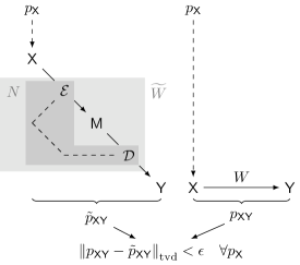
Figure 6: The task of channel simulation with the help of shared randomness

In this section, we extend our discussion to channel simulations with no-signaling correlations. No-signaling channel simulations have been studied in different setups (see, e.g., [12, 42]). In our case, we consider the problem of simulating a channel $W_{\mathsf{Y}|\mathsf{X}}\in\mathcal{P}(\mathcal{Y}|\mathcal{X})$ using a pair no-singling correlated encoder and decoder, namely their joint encoder-decoder map $N_{\mathsf{IY}|\mathsf{XJ}}\in\mathcal{P}(\mathcal{I}\times\mathcal{Y}|\mathcal{X}\times\mathcal{J})$ satisfies the following two conditions (see Fig. 6)

$$\sum_{y\in\mathcal{Y}}N_{\mathsf{IY}|\mathsf{XJ}}(i,y|x,j) =N_{\mathsf{I}|\mathsf{X}}(i|x) \forall j\in\mathcal{J},$$ (97)

$$\sum_{i\in\mathcal{I}}N_{\mathsf{IY}|\mathsf{XJ}}(i,y|x,j) =N_{\mathsf{Y}|\mathsf{J}}(y|j) \forall x\in\mathcal{X}.$$ (98)

Both non-correlated and randomness-assisted simulations are special cases of no-signaling simulations: For non-correlated codes, their joint encoder-decoder maps are in a product form of $\mathcal{E}(i|x)\cdot\mathcal{D}(y|j)$ where $\mathcal{E}$ and $\mathcal{D}$ are the encoding and the decoding functions (or conditional pmfs) of the code. The randomness-assisted channel simulation scheme described in Section I has joint encoder-decoder map in the following form

$$N_{\mathsf{IY}|\mathsf{XJ}}(i,y|x,j)=\sum_{s\in\mathcal{S}}p_{\mathsf{S}}(s)\cdot\mathcal{E}_{s}(i|x)\cdot\mathcal{D}_{s}(y|j).$$ (99)

Another example of a no-signaling resource is a pair of shared entanglement. Given a fixed communication cost $c$ (in terms of alphabet size), we denote $\epsilon^{\mathrm{NS}}(W_{\mathsf{Y}|\mathsf{X}},c)$ the minimal deviation (in TVD) for simulating $W_{\mathsf{Y}|\mathsf{X}}$ using a no-signaling code of size at most $c$. On the other hand, given a fixed deviation-tolerance $\epsilon$ (in TVD), we denote $C^{\mathrm{NS}}(W_{\mathsf{Y}|\mathsf{X}},\epsilon)$ the minimal alphabet size of a no-signaling code simulating $W_{\mathsf{Y}|\mathsf{X}}$ within TVD-tolerance $\epsilon$. In the remainder of this section, we first express $\epsilon^{\mathrm{NS}}(W_{\mathsf{Y}|\mathsf{X}},c)$ and $C^{\mathrm{NS}}(W_{\mathsf{Y}|\mathsf{X}},\epsilon)$ as linear programs, and then relate the latter to our results in the previous sections.

Proposition 10.

Let $W_{\mathsf{Y}|\mathsf{X}}\in\mathcal{P}(\mathcal{Y}|\mathcal{X})$ be a DMC. For any integer $c\geqslant 2$, it holds that

$$\begin{aligned} \epsilon^{\mathrm{NS}}(W_{\mathsf{Y}|\mathsf{X}},c)=\inf\ &\gamma\\ \mathrm{s.t.}\ &\mu_{\mathsf{XY}}\in\mathbb{R}^{\mathcal{X}\times\mathcal{Y}}\\ &\sum_{y\in\mathcal{Y}}\mu_{\mathsf{XY}}(x,y)\leqslant\gamma\quad\forall x\in\mathcal{X}\\ &\mu_{\mathsf{XY}}(x,y)\geqslant\widetilde{W}_{\mathsf{Y}|\mathsf{X}}(y|x)-W_{\mathsf{Y}|\mathsf{X}}(y|x)\quad\forall(x,y)\in\mathcal{X}\times\mathcal{Y}\\ &\widetilde{W}_{\mathsf{Y}|\mathsf{X}}\in\mathcal{P}(\mathcal{Y}|\mathcal{X})\\ &\widetilde{W}_{\mathsf{Y}|\mathsf{X}}(y|x)\leqslant\zeta(y)\quad\forall(x,y)\in\mathcal{X}\times\mathcal{Y}\\ &\sum_{y\in\mathcal{Y}}\zeta(y)=c\end{aligned}.$$ (100)

Moreover, for any $\epsilon\in(0,1)$, it holds that

$$C^{\mathrm{NS}}(W_{\mathsf{Y}|\mathsf{X}},\epsilon) =\begin{aligned} \inf\ &\left\lceil\sum_{y\in\mathcal{Y}}\zeta(y)\right\rceil\\ \mathrm{s.t.}\ &\widetilde{W}_{\mathsf{Y}|\mathsf{X}}\in\mathcal{P}(\mathcal{Y}|\mathcal{X})\\ &\left\lVert\widetilde{W}_{\mathsf{Y}|\mathsf{X}}-W_{\mathsf{Y}|\mathsf{X}}\right\rVert_{\mathrm{tvd}}\leqslant\epsilon\\ &\widetilde{W}_{\mathsf{Y}|\mathsf{X}}(y|x)\leqslant\zeta(y)\quad\forall(x,y)\in\mathcal{X}\times\mathcal{Y}\end{aligned}$$ (101)

$$=\inf_{\widetilde{W}_{\mathsf{Y}|\mathsf{X}}:\left\lVert\widetilde{W}_{\mathsf{Y}|\mathsf{X}}-W_{\mathsf{Y}|\mathsf{X}}\right\rVert_{\mathrm{tvd}}\leqslant\epsilon}\ \left\lceil\sum_{y\in\mathcal{Y}}\max_{x\in\mathcal{X}}\widetilde{W}_{\mathsf{Y}|\mathsf{X}}(y|x)\right\rceil.$$ (102)

Proposition 10 could in principle be deduced from the results in [12], where the authors expressed the cost of no-signaling quantum channel simulation as a semi-definite program (cf. [12, App. A]. However, we give a self-contained proof here in the framework of classical information theory.

Proof of (100).

We start by expressing the minimum deviation (in TVD) for simulating DMC $W_{\mathsf{Y}|\mathsf{X}}\in\mathcal{P}(\mathcal{Y}|\mathcal{X})$ within some fixed communication cost $c\geqslant 2$ as the following linear program

$$\begin{aligned} \epsilon^{\mathrm{NS}}(W_{\mathsf{Y}|\mathsf{X}},c)=\inf\ &\max_{x}\left\lVert W_{\mathsf{Y}|\mathsf{X}}(\cdot|x)-\sum_{i\in\mathcal{M}}N_{\mathsf{IY}|\mathsf{XJ}}(i,\cdot|x,i)\right\rVert_{\mathrm{tvd}}\\ \mathrm{s.t.}\ &N_{\mathsf{IY}|\mathsf{XJ}}\in\mathcal{P}(\mathcal{M}\times\mathcal{Y}|\mathcal{X}\times\mathcal{M})\\ &\sum_{y\in\mathcal{Y}}N_{\mathsf{IY}|\mathsf{XJ}}(i,y|x,j)=N_{\mathsf{I}|\mathsf{X}}(i|x)\quad\forall j\in\mathcal{J}\\ &\sum_{i\in\mathcal{M}}N_{\mathsf{IY}|\mathsf{XJ}}(i,y|x,j)=N_{\mathsf{Y}|\mathsf{J}}(y|j)\quad\forall x\in\mathcal{X}\\ &\left\lvert\mathcal{M}\right\rvert=c\end{aligned}.$$ (103)

Notice that one can rewrite the TVD-distance between channels as

$$\left\lVert W_{\mathsf{Y}|\mathsf{X}}-\widetilde{W}_{\mathsf{Y}|\mathsf{X}}\right\rVert_{\mathrm{tvd}} =\max_{x\in\mathcal{X}}\left\lVert W_{\mathsf{Y}|\mathsf{X}}(\cdot|x)-\widetilde{W}_{\mathsf{Y}|\mathsf{X}}(\cdot|x)\right\rVert_{\mathrm{tvd}}=\frac{1}{2}\max_{x\in\mathcal{X}}\left\lVert W_{\mathsf{Y}|\mathsf{X}}(\cdot|x)-\widetilde{W}_{\mathsf{Y}|\mathsf{X}}(\cdot|x)\right\rVert_{1}$$ (104)

$$=\inf\left\{\gamma\in\mathbb{R}\middle|\mu_{\mathsf{XY}}\in\mathbb{R}_{\geqslant 0}^{\mathcal{X}\times\mathcal{Y}},\sum_{y\in\mathcal{Y}}\mu_{\mathsf{XY}}(\cdot,y)\leqslant\gamma,\mu_{\mathsf{XY}}\geqslant\widetilde{W}_{\mathsf{Y}|\mathsf{X}}-W_{\mathsf{Y}|\mathsf{X}}\right\}.$$ (105)

This enables us to rewrite (103) as

$$\begin{aligned} \epsilon^{\mathrm{NS}}(W_{\mathsf{Y}|\mathsf{X}},c)=\inf\ &\gamma\\ \mathrm{s.t.}\ &\mu_{\mathsf{XY}}\in\mathbb{R}_{\geqslant 0}^{\mathcal{X}\times\mathcal{Y}}\\ &\sum_{y\in\mathcal{Y}}\mu_{\mathsf{XY}}(x,y)\leqslant\gamma\quad\forall x\in\mathcal{X}\\ &\mu_{\mathsf{XY}}(x,y)\geqslant\sum_{i\in\mathcal{M}}N_{\mathsf{IY}|\mathsf{XJ}}(i,y|x,i)-W_{\mathsf{Y}|\mathsf{X}}(y|x)\quad\forall(x,y)\in\mathcal{X}\times\mathcal{Y}\\ &N_{\mathsf{IY}|\mathsf{XJ}}\in\mathcal{P}(\mathcal{M}\times\mathcal{Y}|\mathcal{X}\times\mathcal{M})\\ &\sum_{y\in\mathcal{Y}}N_{\mathsf{IY}|\mathsf{XJ}}(i,y|x,j)=N_{\mathsf{I}|\mathsf{X}}(i|x)\quad\forall j\in\mathcal{J}\\ &\sum_{i\in\mathcal{M}}N_{\mathsf{IY}|\mathsf{XJ}}(i,y|x,j)=N_{\mathsf{Y}|\mathsf{J}}(y|j)\quad\forall x\in\mathcal{X}\\ &\left\lvert\mathcal{M}\right\rvert=c\end{aligned}.$$ (106)

It remains to show (106) to be equivalent to (100). We first show that for any feasible $\widetilde{W}_{\mathsf{Y}|\mathsf{X}}$ and $\zeta$ for (100), one can construct some $N_{\mathsf{IY}|\mathsf{XJ}}\in\mathcal{P}(\mathcal{M}\times\mathcal{Y}|\mathcal{X}\times\mathcal{M})$ satisfying the conditions in (106) such that

$$\widetilde{W}_{\mathsf{Y}|\mathsf{X}}(y|x)=\sum_{i\in\mathcal{M}}N_{\mathsf{IY}|\mathsf{XJ}}(i,y|x,i)\quad\forall(x,y)\in\mathcal{X}\times\mathcal{Y}.$$ (107)

This can be shown by constructing $N_{\mathsf{IY}|\mathsf{XJ}}$ as

$$N_{\mathsf{IY}|\mathsf{XJ}}(i,y|x,j)=\begin{cases}\frac{\widetilde{W}_{\mathsf{Y}|\mathsf{X}}(y|x)}{c}&\text{for $i=j$}\\ \frac{\zeta(y)-\widetilde{W}_{\mathsf{Y}|\mathsf{X}}(y|x)}{c(c-1)}&\text{for $i\neq j$}\end{cases}.$$ (108)

It is straightforward to check that $\sum_{i\in\mathcal{M}}N_{\mathsf{IY}|\mathsf{XJ}}(i,y|x,i)=\widetilde{W}_{\mathsf{Y}|\mathsf{X}}(y|x)$. Since that $\zeta(y)\geqslant W_{\mathsf{Y}|\mathsf{X}}(y|x)$ and that $c\geqslant 2$ we know $N_{\mathsf{IY}|\mathsf{XJ}}$ to be non-negative. To verify $N_{\mathsf{IY}|\mathsf{XJ}}$ to be a conditional pmf, we have

$$\sum_{i\in\mathcal{M},y\in\mathcal{Y}}N_{\mathsf{IY}|\mathsf{XJ}}(i,y|x,j)=\sum_{y}\left(\frac{\widetilde{W}_{\mathsf{Y}|\mathsf{X}}(y|x)}{c}+\frac{\zeta(y)-\widetilde{W}_{\mathsf{Y}|\mathsf{Y}}(y|x)}{c(c-1)}\cdot(c-1)\right)=\sum_{y\in\mathcal{Y}}\frac{\zeta(y)}{c}=1.$$ (109)

To verify $N_{\mathsf{IY}|\mathsf{XJ}}$ to be no-signaling, we have

$$\sum_{y\in\mathcal{Y}}N_{\mathsf{IY}|\mathsf{XJ}}(i,y|x,j) =\frac{1}{c} \forall j\in\mathcal{M},$$ (110)

$$\sum_{i\in\mathcal{M}}N_{\mathsf{IY}|\mathsf{XJ}}(i,y|x,j) =\frac{\widetilde{W}_{\mathsf{Y}|\mathsf{X}}(y|x)}{c}+\sum_{i\neq j}\frac{\zeta(y)-\widetilde{W}_{\mathsf{Y}|\mathsf{X}}(y|x)}{c(c-1)}=\frac{\zeta(y)}{c} \forall x\in\mathcal{X}.$$ (111)

On the other hand, suppose $N_{\mathsf{IY}|\mathsf{XJ}}$ being some feasible no-signaling conditional pmf for (106), we claim that $\widetilde{W}_{\mathsf{Y}|\mathsf{X}}$ and $\zeta$ defined below are feasible for (100):

$$\widetilde{W}_{\mathsf{Y}|\mathsf{X}}(y|x) \coloneqq\sum_{i\in\mathcal{M}}N_{\mathsf{IY}|\mathsf{XJ}}(i,y|x,i) \forall(x,y)\in\mathcal{X}\times\mathcal{Y},$$ (112)

$$\zeta(y) \coloneqq\sum_{j\in\mathcal{M}}N_{\mathsf{Y}|\mathsf{J}}(y|j) \forall y\in\mathcal{Y}.$$ (113)

Since it is straightforward to check $\widetilde{W}_{\mathsf{Y}|\mathsf{X}}$ to be a conditional pmf and that $\sum_{y}\zeta(y)=c$, it remains to verify $\widetilde{W}_{\mathsf{Y}|\mathsf{X}}(y|x)\leqslant\zeta(y)$ for all $y\in\mathcal{Y}$, which is indeed the case since

$$\widetilde{W}_{\mathsf{Y}|\mathsf{X}}(y|x)=\sum_{i\in\mathcal{M}}N_{\mathsf{IY}|\mathsf{XJ}}(i,y|x,i)\leqslant\sum_{i,j\in\mathcal{M}}N_{\mathsf{IY}|\mathsf{XJ}}(i,y|x,j)=\sum_{j\in\mathcal{M}}N_{\mathsf{Y}|\mathsf{J}}(y|j)=\zeta(y).$$ (114)

Combining the above two arguments, we have established the equivalence between (106) and (100). ∎

Proof of (101).

As a direct result of (100), we know a tolerance-cost pair $(\epsilon,c)$ (where the integer $c\geqslant 2$) is attainable for if and only if their exists some $\mu_{\mathsf{XY}}\in\mathbb{R}_{\geqslant 0}^{\mathcal{X}\times\mathcal{Y}}$ and $\widetilde{W}_{\mathsf{Y}|\mathsf{X}}\in\mathcal{P}(\mathcal{Y}|\mathcal{X})$ such that

$$\sum_{y\in\mathcal{Y}}\mu_{\mathsf{XY}}(x,y) \leqslant\epsilon \forall x\in\mathcal{X}$$ (115)

$$\mu_{\mathsf{XY}}(x,y) \geqslant\widetilde{W}_{\mathsf{Y}|\mathsf{X}}(y|x)-W_{\mathsf{Y}|\mathsf{X}}(y|x) \forall(x,y)\in\mathcal{X}\times\mathcal{Y}$$ (116)

$$\widetilde{W}_{\mathsf{Y}|\mathsf{X}}(y|x) \leqslant\zeta(y) \forall(x,y)\in\mathcal{X}\times\mathcal{Y}$$ (117)

$$\sum_{y\in\mathcal{Y}}\zeta(y) =c.$$ (118)

Thus, for a given deviation $\epsilon$ (in TVD), one can express the minimal communication cost achieving such deviation as the following optimization problem.

$$\begin{aligned} C^{\mathrm{NS}}(W_{\mathsf{Y}|\mathsf{X}},\epsilon)=\inf\ &\left\lceil\sum_{y\in\mathcal{Y}}\zeta(y)\right\rceil\\ \mathrm{s.t.}\ &\mu_{\mathsf{XY}}\in\mathbb{R}^{\mathcal{X}\times\mathcal{Y}}\\ &\sum_{y\in\mathcal{Y}}\mu_{\mathsf{XY}}(x,y)\leqslant\epsilon\quad\forall x\in\mathcal{X}\\ &\mu_{\mathsf{XY}}(x,y)\geqslant\widetilde{W}_{\mathsf{Y}|\mathsf{X}}(y|x)-W_{\mathsf{Y}|\mathsf{X}}(y|x)\quad\forall(x,y)\in\mathcal{X}\times\mathcal{Y}\\ &\widetilde{W}_{\mathsf{Y}|\mathsf{X}}\in\mathcal{P}(\mathcal{Y}|\mathcal{X})\\ &\widetilde{W}_{\mathsf{Y}|\mathsf{X}}(y|x)\leqslant\zeta(y)\quad\forall(x,y)\in\mathcal{X}\times\mathcal{Y}\end{aligned}.$$ (119)

Using (105), we can simplify the above linear program into (101). ∎

In the following, we show how $C^{\mathrm{NS}}(W_{\mathsf{Y}|\mathsf{X}},\epsilon)$ as in (102) is related to the cost of the random-assisted channel simulation. In particular, we have the following theorem.

Theorem 11.

Let $W_{\mathsf{Y}|\mathsf{X}}$ be a DMC from $\mathcal{X}$ to $\mathcal{Y}$, and let $\epsilon\in(0,1)$. Let $C^{\mathrm{NS}}(W_{\mathsf{Y}|\mathsf{X}},\epsilon)$ denote the minimal attainable size of no-signaling $\epsilon$-simulation codes for $W_{\mathsf{Y}|\mathsf{X}}$, then

$$\log{C^{\mathrm{NS}}(W_{\mathsf{Y}|\mathsf{X}},\epsilon)}=\left\lceil I_{\max}^{\epsilon}(W_{\mathsf{Y}|\mathsf{X}})\right\rceil_{\log{\mathbb{Z}_{>0}}}$$ (120)

where for any $r\in\mathbb{R}$ we denote $\left\lceil r\right\rceil_{\log{\mathbb{Z}_{>0}}}$ the smallest number in $\log{\mathbb{Z}_{>0}}\coloneqq\left\{\log{a}:a\in\mathbb{Z},a>0\right\}$ that is no smaller than $r$.

Compare the RHS of (120) with (44). We see that the task of no-signaling channel simulations is no more difficult than the random-assisted channel simulation. Since, in the $n$-fold case for the random-assisted channel simulation, the converse bounds as in (44) is tight up to the second order expansion term, no-signaling channel simulations must also have the same first and second order term in the expansions. To prove Theorem 11, we need the following lemma.

Lemma 12.

Let $\mathcal{X}$ be a finite set, and $f$ be a non-negative valued function on $\mathcal{X}$. It holds that

$$\inf_{p\in\mathcal{P}(\mathcal{X})}\max_{x\in\mathcal{X}}\frac{f(x)}{p(x)}=\sum_{x\in\mathcal{X}}f(x).$$ (121)

Proof.

See Appendix A. ∎

Proof of Theorem 11.

Let $W_{\mathsf{Y}|\mathsf{X}}$ be a DMC from $\mathcal{X}$ to $\mathcal{Y}$, and let $\epsilon\in(0,1)$. Starting from (102), we have the following chain of identities:

$$C^{\mathrm{NS}}(W_{\mathsf{Y}|\mathsf{X}},\epsilon)=\inf_{\widetilde{W}_{\mathsf{Y}|\mathsf{X}}:\left\lVert\widetilde{W}_{\mathsf{Y}|\mathsf{X}}-W_{\mathsf{Y}|\mathsf{X}}\right\rVert_{\mathrm{tvd}}\leqslant\epsilon}\ \left\lceil\sum_{y\in\mathcal{Y}}\max_{x\in\mathcal{X}}\widetilde{W}_{\mathsf{Y}|\mathsf{X}}(y|x)\right\rceil\hskip 147.0pt\text{copied from~{}\eqref{eq:NS:LP:c:eps:1}}$$ (122)

$$\phantom{C^{\mathrm{NS}}(W_{\mathsf{Y}|\mathsf{X}},\epsilon)}=\left\lceil\inf_{\widetilde{W}_{\mathsf{Y}|\mathsf{X}}:\left\lVert\widetilde{W}_{\mathsf{Y}|\mathsf{X}}-W_{\mathsf{Y}|\mathsf{X}}\right\rVert_{\mathrm{tvd}}\leqslant\epsilon}\ \sum_{y\in\mathcal{Y}}\max_{x\in\mathcal{X}}\widetilde{W}_{\mathsf{Y}|\mathsf{X}}(y|x)\right\rceil\hskip 146.0pt\text{see the text below}$$ (123)

$$\phantom{C^{\mathrm{NS}}(W_{\mathsf{Y}|\mathsf{X}},\epsilon)}=\left\lceil\multiadjustlimits{\inf_{\widetilde{W}_{\mathsf{Y}|\mathsf{X}}:\left\lVert\widetilde{W}_{\mathsf{Y}|\mathsf{X}}-W_{\mathsf{Y}|\mathsf{X}}\right\rVert_{\mathrm{tvd}}\leqslant\epsilon},\inf_{q_{\mathsf{Y}}\in\mathcal{P}(\mathcal{Y})},\max_{y\in\mathcal{Y}}}\frac{\max_{x\in\mathcal{X}}\widetilde{W}_{\mathsf{Y}|\mathsf{X}}(y|x)}{q_{\mathsf{Y}}(y)}\right\rceil\hskip 111.0pt\text{by Lemma~{}\ref{lem:inf:max}}$$ (124)

$$\phantom{C^{\mathrm{NS}}(W_{\mathsf{Y}|\mathsf{X}},\epsilon)}=\left\lceil\multiadjustlimits{\inf_{q_{\mathsf{Y}}\in\mathcal{P}(\mathcal{Y})},\inf_{\widetilde{W}_{\mathsf{Y}|\mathsf{X}}:\left\lVert\widetilde{W}_{\mathsf{Y}|\mathsf{X}}-W_{\mathsf{Y}|\mathsf{X}}\right\rVert_{\mathrm{tvd}}\leqslant\epsilon},\max_{x\in\mathcal{X}}}2^{D_{\max}\left(\widetilde{W}_{\mathsf{Y}|\mathsf{X}}(\cdot|x)\middle\|q_{\mathsf{Y}}\right)}\right\rceil\hskip 67.0pt\text{by the definition of }D_{\max}$$ (125)

$$\phantom{C^{\mathrm{NS}}(W_{\mathsf{Y}|\mathsf{X}},\epsilon)}=\left\lceil 2^{\multiadjustlimits{\inf_{q_{\mathsf{Y}}\in\mathcal{P}(\mathcal{Y})},\inf_{\widetilde{W}_{\mathsf{Y}|\mathsf{X}}:\left\lVert\widetilde{W}_{\mathsf{Y}|\mathsf{X}}-W_{\mathsf{Y}|\mathsf{X}}\right\rVert_{\mathrm{tvd}}\leqslant\epsilon},\max_{x\in\mathcal{X}}}D_{\max}\left(\widetilde{W}_{\mathsf{Y}|\mathsf{X}}(\cdot|x)\middle\|q_{\mathsf{Y}}\right)}\right\rceil\hskip 69.0ptx\mapsto 2^{x}\text{ is strictly increasing}$$ (126)

where (123) is due to the compactness of $\left\{\widetilde{W}_{\mathsf{Y}|\mathsf{X}}:\left\lVert\widetilde{W}_{\mathsf{Y}|\mathsf{X}}-W_{\mathsf{Y}|\mathsf{X}}\right\rVert_{\mathrm{tvd}}\leqslant\epsilon\right\}$ and the continuity of the function $\widetilde{W}_{\mathsf{Y}|\mathsf{X}}\mapsto\sum_{y\in\mathcal{Y}}\max_{x\in\mathcal{X}}\widetilde{W}_{\mathsf{Y}|\mathsf{X}}(y|x)$. Notice that the logarithm function is increasing. Hence, we can take logarithm on both sides of the inequality and get

$$\log{C^{\mathrm{NS}}(W_{\mathsf{Y}|\mathsf{X}},\epsilon)}=\left\lceil\multiadjustlimits{\inf_{q_{\mathsf{Y}}\in\mathcal{P}(\mathcal{Y})},\inf_{\widetilde{W}_{\mathsf{Y}|\mathsf{X}}:\left\lVert\widetilde{W}_{\mathsf{Y}|\mathsf{X}}-W_{\mathsf{Y}|\mathsf{X}}\right\rVert_{\mathrm{tvd}}\leqslant\epsilon},\max_{x\in\mathcal{X}}}D_{\max}\left(\widetilde{W}_{\mathsf{Y}|\mathsf{X}}(\cdot|x)\middle\|q_{\mathsf{Y}}\right)\right\rceil_{\log{\mathbb{Z}_{>0}}}=\left\lceil I_{\max}^{\epsilon}(W_{\mathsf{Y}|\mathsf{X}})\right\rceil_{\log{\mathbb{Z}_{>0}}}.\qed$$

Example: $n$-fold binary symmetric channel

We now investigate the case of simulating i.i.d. copies of a binary symmetric channel with crossover probability $\delta$. In this case, the linear programs (100) and (119) simplify considerably. We have

$$W_{\mathsf{Y}^{n}|\mathsf{X}^{n}}=\begin{pmatrix}1-\delta&\delta\\ \delta&1-\delta\end{pmatrix}^{\otimes n}$$ (127)

For $n,k\in\mathbb{N}$ and $0\leqslant k\leqslant n$, let $P^{n}_{k}(I,X)$ refer to the binary matrix obtained by the sum of all $n$-fold tensor factors of $I$ and $X$, where $I=\left(\begin{smallmatrix}1&0\\ 0&1\end{smallmatrix}\right)$ and $X=\left(\begin{smallmatrix}0&1\\ 1&0\end{smallmatrix}\right)$, with exactly $k$ factors of $X$. For instance, $P^{3}_{1}(I,X)=I\otimes I\otimes X+I\otimes X\otimes I+X\otimes I\otimes I$. We make the following observations

• $W_{\mathsf{Y}^{n}|\mathsf{X}^{n}}=((1-\delta)I+\delta X)^{\otimes n}=\sum_{k=0}^{n}(1-\delta)^{n-k}\delta^{k}\cdot P^{n}_{k}(I,X)$.

• The symmetries of $W_{\mathsf{Y}^{n}|\mathsf{X}^{n}}$ allow us to choose $\widetilde{W}_{\mathsf{Y}^{n}|\mathsf{X}^{n}}=\sum_{k=0}^{n}r_{k}P^{n}_{k}(I,X)$, $p_{\mathsf{XY}}=\sum_{k=0}^{n}y_{k}P^{n}_{k}(I,X)$ and $\zeta(y)=s$, where $s$ is some constant without loss of generality.

• The set of matrices $\{P^{n}_{1}(I,X),P^{n}_{2}(I,X),...,P^{n}_{n}(I,X)\}\}$ form a “partition” of the entries of a $2^{n}\times 2^{n}$ matrix. That is, $\sum_{k=0}^{n}P^{n}_{k}(I,X)=J_{2^{n}}$, where $J_{m}$ is the $m\times m$ matrix with all entries equal to $1$. Additionally, since for each $k$, $P^{n}_{k}(I,X)$ is a $2^{n}\times 2^{n}$ binary matrix, it also holds that if $P^{n}_{k}(I,X)(i,j)=1$, then $P^{n}_{k^{\prime}}(I,X)(i,j)=0$ for all $k\neq k^{\prime}$ and for all $i,j$.

These observations allow us to simplify the linear program in (100) for an $n$-fold binary symmetric channel with crossover probability $\delta$ as follows.

$$\epsilon^{\mathrm{NS}}(W_{\mathsf{Y}^{n}|\mathsf{X}^{n}},c)=\inf \gamma$$ (128)

$$\mathrm{s.t.} y_{k}\geqslant 0\quad\forall k$$

$$\sum_{k=0}^{n}\binom{n}{k}y_{k}\leqslant\gamma$$

$$y_{k}\geqslant r_{k}-(1-\delta)^{n-k}\delta^{k}\quad\forall k$$

$$\sum_{k=0}^{n}\binom{n}{k}r_{k}=1$$

$$0\leqslant r_{k}\leqslant s\quad\forall k$$

$$2^{n}s=c.$$

Similarly, we can simplify (119) as follows.

$$C^{\mathrm{NS}}(W_{\mathsf{Y}^{n}|\mathsf{X}^{n}},\epsilon)=\inf \left\lceil 2^{n}s\right\rceil$$ (129)

$$\mathrm{s.t.} y_{k}\geqslant 0\ \quad\forall k$$

$$\sum_{k=0}^{n}\binom{n}{k}y_{k}\leqslant\epsilon$$

$$y_{k}\geqslant r_{k}-(1-\delta)^{n-k}\delta^{k}\quad\forall k$$

$$0\leqslant r_{k}\leqslant s\quad\forall k$$

$$\sum_{k=0}^{n}\binom{n}{k}r_{k}=1$$

In Figure 2 in the introduction, we solve the linear program in (129) for a binary symmetric channel with $\delta=0.1$ and $\epsilon=0.05$. The second-order approximation of the simulation cost, the capacity of the channel and a finite blocklength converse bound on the capacity are also shown.

V Generalization to Broadcast Channels

In this section, we consider the problem of simulating broadcast channels with unconstrained shared randomness between the sender and each of the receivers. Given a broadcast channel $W_{\mathbf{\mathsf{Y}}_{1}^{K}|\mathsf{X}}\in\mathcal{P}(\mathcal{Y}_{1}\times\cdots\times\mathcal{Y}_{K}|\mathcal{X})$ and independent random variables $\{\mathsf{S}_{i}\}_{i=1,\ldots,K}$, each shared between the sender and the $i$-th receiver, respectively, the task of simulating $W_{\mathbf{\mathsf{Y}}_{1}^{K}|\mathsf{X}}$ within a tolerance of $\epsilon$ in TVD is to find encoders $\{\mathcal{E}_{s_{i}}^{(i)}\in\mathcal{P}([M_{i}]|\mathcal{X})\}_{i=1,\ldots,K}$ and decoders $\{\mathcal{D}_{s_{i}}^{(i)}\in\mathcal{P}(\mathcal{Y}_{i}|[M_{i}])\}_{i=1,\ldots,K}$ such that, for all input distributions $p_{\mathsf{X}}\in\mathcal{P}(\mathcal{X})$, the induced joint distribution

$$\widetilde{p}_{\mathsf{X}\mathbf{\mathsf{Y}}_{1}^{K}}(x,\mathbf{y}_{1}^{K})\coloneqq p_{\mathsf{X}}(x)\cdot\sum_{\mathbf{s}_{1}^{K}\in\mathcal{S}_{1}\times\cdots\times\mathcal{S}_{K}}\prod_{i=1}^{K}p_{\mathsf{S}_{i}}(s_{i})\cdot\sum_{\mathbf{m}_{1}^{K}\in[M_{1}]\times\cdots\times[M_{K}]}\prod_{i=1}^{K}\mathcal{E}_{s_{i}}^{(i)}(m_{i}|x)\cdot\prod_{i=1}^{K}\mathcal{D}_{s_{i}}^{(i)}(y_{i}|m_{i})$$ (130)

is $\epsilon$-close to the original joint distribution $p_{\mathsf{X}\mathbf{\mathsf{Y}}_{1}^{K}}(x,\mathbf{y}_{1}^{K})\coloneqq p_{\mathsf{X}}(x)\cdot W_{\mathbf{\mathsf{Y}}_{1}^{K}|\mathsf{X}}(\mathbf{y}_{1}^{K}|x)$ in TVD. Here, $[M]\coloneqq\{1,\ldots,M\}$ for each positive integer $M$. Using a similar notion as in the point-to-point case, we refer to $(\{\mathcal{E}_{s_{i}}^{(i)}\}_{s\in\mathcal{S}_{i},i=1,\ldots,K},\{\mathcal{D}_{s_{i}}^{(i)}\}_{s\in\mathcal{S}_{i},i=1,\ldots,K},\mathbf{\mathsf{S}}_{1}^{K})$ as a size-$\mathbf{M}_{1}^{K}$ $\epsilon$-simulation code for $W_{\mathbf{\mathsf{Y}}_{1}^{K}|\mathsf{X}}$. Fig. 3 depicts the scenario when $K=2$.

Under similar notions, a $K$-tuple $\mathbf{M}_{1}^{K}=(M_{1},\ldots,M_{K})$ is said to be $\epsilon$-attainable if there exists a size-$\mathbf{M}_{1}^{K}$ $\epsilon$-simulation code. As a first observation, if $(M_{1},\ldots,M_{K})$ is attainable, so is $(M_{1}^{+},\ldots,M_{K}^{+})$ for any integers $M_{1}^{+}\geqslant M_{1},\ldots,M_{K}^{+}\geqslant M_{K}$. Given a $K$-receiver broadcast channel $W_{\mathbf{\mathsf{Y}}_{1}^{K}|\mathsf{X}}$, we denote $\mathcal{M}^{\star}_{\epsilon}(W_{\mathbf{\mathsf{Y}}_{1}^{K}|\mathsf{X}})$ the set of all $\epsilon$-attainable message-size tuples. In this section, we develop a pair of subset and superset for $\mathcal{M}^{\star}_{\epsilon}(W_{\mathbf{\mathsf{Y}}_{1}^{K}|\mathsf{X}})$.

V-A One-Shot Achievability Bound

Differently from the point-to-point case, we propose an achievability bound based on the multipartite convex split lemma as described below.

Lemma 13 ($K$-partite Convex Split Lemma [23, Fact 7, modified]).

Let $K$ be a positive integer and $\epsilon\in(0,1)$. For each nonempty subset $\mathcal{J}$ of $\{1,\ldots,K\}$, let $\delta_{\mathcal{J}}\in(0,1)$, and suppose

$$\sum_{\mathcal{J}\subset\{1,\ldots,K\}:\mathcal{J\neq\emptyset}}\delta_{\mathcal{J}}^{2}\leqslant\epsilon^{2}.$$ (131)

Let $(\mathsf{X},\mathsf{Y}_{1},\ldots,\mathsf{Y}_{K})$ be jointly distributed over $\mathcal{X}\times\mathcal{Y}_{1}\times\cdots\times\mathcal{Y}_{K}$ with pmf $p_{\mathsf{X}\mathbf{\mathsf{Y}}_{1}^{K}}$. For each $i\in\{1,\ldots,K\}$, let $q_{\mathsf{Y}_{i}}$ be a pmf over $\mathcal{Y}_{i}$. (Note that in general $q_{\mathsf{Y}_{i}}\neq q_{\mathsf{Y}_{j}}$ for $i\neq j$.) Let $\mathbf{M}_{1}^{K}=(M_{1},\ldots,M_{K})$ be a $K$-length vector of positive integers such that for all nonempty subset $\mathcal{J}$ of $\{1,\ldots,K\}$

$$\sum_{i\in\mathcal{J}}\log{M}_{i}\geqslant D_{s+}^{\epsilon_{\mathcal{J}}}\left(p_{\mathsf{X}\mathbf{\mathsf{Y}}_{\mathcal{J}}}\middle\|p_{\mathsf{X}}\times\prod_{i\in\mathcal{J}}q_{\mathsf{Y}_{i}}\right)-\log{\delta_{\mathcal{J}}^{2}}$$ (132)

for some $\{\epsilon_{\mathcal{J}}\}_{\mathcal{J}\subset\{1,\ldots,K\}:\mathcal{J}\neq\emptyset}$ such that

$$\sum_{\mathcal{J}\subset\{1,\ldots,K\}:\mathcal{J}\neq\emptyset}\epsilon_{\mathcal{J}}\leqslant\epsilon-\sqrt{\sum_{\mathcal{J}\subset\{1,\ldots,K\}:\mathcal{J}\neq\emptyset}\delta_{\mathcal{J}}^{2}}.$$ (133)

For each $i\in\{1,\ldots,K\}$, let $\mathsf{J}_{i}$ be independently uniformly distributed on $\{1,\ldots,M_{i}\}$. Let the joint random variables $(\mathbf{\mathsf{J}}_{1}^{K},\mathsf{X},\mathbf{\mathsf{Y}}_{1,1}^{M_{1}},\ldots,\mathbf{\mathsf{Y}}_{K,1}^{M_{K}})$ be distributed according to

$$p_{\mathsf{X},\mathbf{\mathsf{Y}}_{1,1}^{M_{1}},\ldots\mathbf{\mathsf{Y}}_{K,1}^{M_{K}}|\mathbf{\mathsf{J}}_{1}^{K}}(x,\mathbf{y}_{1,1}^{M_{1}},\ldots,\mathbf{y}_{K,1}^{M_{K}}|\mathbf{j}_{1}^{K})=p_{\mathsf{X}\mathbf{\mathsf{Y}}_{1}^{K}}(x,y_{1,j_{1}},\ldots,y_{K,j_{K}})\cdot\prod_{i=1}^{K}\prod_{j\in\{1,\ldots,M_{i}\}\setminus\{j_{i}\}}q_{\mathsf{Y}_{i}}(y_{i,j}).$$ (134)

Then,

$$\left\lVert p_{\mathsf{X},\mathbf{\mathsf{Y}}_{1,1}^{M_{1}},\ldots,\mathbf{\mathsf{Y}}_{K,1}^{M_{K}}}-p_{\mathsf{X}}\times\prod_{i=1}^{K}\prod_{j=1}^{M_{i}}q_{\mathsf{Y}_{i,j}}\right\rVert_{\mathrm{tvd}}\leqslant\epsilon$$ (135)

where for each $i=1,\ldots,K$, $q_{\mathsf{Y}_{i,j}}=q_{\mathsf{Y}_{i}}$ for all $j=1,\ldots,M_{i}$.

Proof.

This lemma can be proven via a rather straightforward generalization of the proof for [23, Fact 7]. For notational simplicity, we only include the proof for the case when $K=2$ in Appendix B. ∎

Proposition 14.

Let $K$ be a positive integer. Let $W_{\mathbf{\mathsf{Y}}_{1}^{K}|\mathsf{X}}$ be a DMC from $\mathcal{X}$ to $\mathcal{Y}_{1}\times\cdots\times\mathcal{Y}_{K}$, and let $\epsilon\in(0,1)$. For each subset $\mathcal{J}$ of $\{1,\ldots,K\}$, let $\epsilon_{\mathcal{J}}$ and $\delta_{\mathcal{J}}<\epsilon_{\mathcal{J}}$ be positive real numbers. Suppose

$$\sum_{\mathcal{J}\subset\{1,\ldots,K\}:\mathcal{J}\neq\emptyset}\epsilon_{\mathcal{J}}\leqslant\epsilon.$$ (136)

Let $q_{\mathsf{Y}_{i}}\in\mathcal{P}(\mathcal{Y}_{i})$ for each $i=1,\ldots,K$. The following set is a subset of $\mathcal{M}^{\star}_{\epsilon}(W_{\mathbf{\mathsf{Y}}_{1}^{K}|\mathsf{X}})$:

$$\mathcal{M}^{\text{in}}_{\epsilon}(W_{\mathbf{\mathsf{Y}}_{1}^{K}|\mathsf{X}})\coloneqq\left\{\mathbf{M}\in\mathbb{Z}_{>0}^{K}\middle|\begin{aligned} \sum_{i\in\mathcal{J}}\log{M_{i}}>D_{s+}^{\epsilon_{\mathcal{J}}-\delta_{\mathcal{J}}}\left(p_{\mathsf{X}}\cdot W_{\mathbf{\mathsf{Y}}_{\mathcal{Y}}|\mathsf{X}}\middle\|p_{\mathsf{X}}\times\prod_{i\in\mathcal{J}}q_{\mathsf{Y}_{i}}\right)-\log{\delta_{\mathcal{J}}^{2}}\\ \forall\mathcal{J}\subset\{1,\ldots,K\}\text{ with }\mathcal{J}\neq\emptyset,\forall p_{\mathsf{X}}\in\mathcal{P}(\mathcal{X})\end{aligned}\right\}.$$ (137)

In particular, for the case when $K=2$, we have

$$\mathcal{M}^{\text{in}}_{\epsilon}(W_{\mathsf{YZ}|\mathsf{X}})\coloneqq\left\{(M,N)\in\mathbb{Z}_{>0}^{2}\middle|\begin{aligned} \log{M}&>D_{s+}^{\epsilon_{1}-\delta_{1}}\left(p_{\mathsf{X}}\cdot W_{\mathsf{Y}|\mathsf{X}}\middle\|p_{\mathsf{X}}\times q_{\mathsf{Y}}\right)-\log{\delta_{1}^{2}}\\ \log{N}&>D_{s+}^{\epsilon_{2}-\delta_{2}}\left(p_{\mathsf{X}}\cdot W_{\mathsf{Z}|\mathsf{X}}\middle\|p_{\mathsf{X}}\times r_{\mathsf{Z}}\right)-\log{\delta_{2}^{2}}\\ \log{MN}&>D_{s+}^{\epsilon_{3}-\delta_{3}}\left(p_{\mathsf{X}}\cdot W_{\mathsf{YZ}|\mathsf{X}}\middle\|p_{\mathsf{X}}\times q_{\mathsf{Y}}\times r_{\mathsf{Z}}\right)-\log{\delta_{3}^{2}}\end{aligned}\quad\forall p_{\mathsf{X}}\in\mathcal{P}(\mathcal{X}),\right\}$$ (138)

where $\epsilon_{1},\epsilon_{2},\epsilon_{3}$ are positive numbers such that $\epsilon_{1}+\epsilon_{2}+\epsilon_{3}\leqslant\epsilon$, $\delta_{1}\in(0,\epsilon_{1})$, $\delta_{2}\in(0,\epsilon_{2})$, $\delta_{3}\in(0,\epsilon_{3})$, $q_{\mathsf{Y}}\in\mathcal{P}(\mathcal{Y})$, $r_{\mathsf{Z}}\in\mathcal{P}(\mathcal{Z})$, and the reduced channels $W_{\mathsf{Y}|\mathsf{X}}$ and $W_{\mathsf{Z}|\mathsf{X}}$ are defined as

$$W_{\mathsf{Y}|\mathsf{X}}(y|x)\coloneqq\sum_{z\in\mathcal{Z}}W_{\mathsf{YZ}|\mathsf{X}}(y,z|x),\quad W_{\mathsf{Z}|\mathsf{X}}(y|x)\coloneqq\sum_{y\in\mathcal{Y}}W_{\mathsf{YZ}|\mathsf{X}}(y,z|x).$$ (139)

For notational simplicity, we only show the case when $K=2$ in the following proof, which can be generalized to generic $K$’s rather straightforwardly.

Proof.

For arbitrary $q_{\mathsf{Y}}\in\mathcal{P}(\mathcal{Y})$, $r_{\mathsf{Z}}\in\mathcal{P}(\mathcal{Z})$, we present a protocol for simulating $W_{\mathsf{YZ}|\mathsf{X}}$ by sending messages with alphabet sizes $M$ and $N$ to each of the receivers, respectively, where $(M,N)$ is any integer pair satisfying the conditions on the RHS of (138). The protocol is as follows:

1. Let the sender and first receiver share i.i.d. random variables $(\mathsf{Y}_{1},\ldots,\mathsf{Y}_{M})$ where $\mathsf{Y}_{k}\sim q_{\mathsf{Y}}$ for each $k$.

2. Let the sender and second receiver share i.i.d. random variables $(\mathsf{Z}_{1},\ldots,\mathsf{Z}_{N})$ where $\mathsf{Z}_{k}\sim r_{\mathsf{Z}}$ for each $k$.

3. Upon receiving input $\mathsf{X}=x$, the sender generates a pair of random variables $\mathsf{J},\mathsf{K}$ (distributed on $\{1,\ldots,M\}\times\{1,\ldots,N\}$) according to the following conditional pmf

   $$\widetilde{p}_{\mathsf{J},\mathsf{K}|\mathsf{X},\mathbf{\mathsf{Y}}_{1}^{M},\mathbf{\mathsf{Z}}_{1}^{N}}(j,k|x,\mathbf{y}_{1}^{M},\mathbf{z}_{1}^{N})\coloneqq\frac{W_{\mathsf{YZ}|\mathsf{X}}(y_{j},z_{k}|x)\cdot\prod_{i\neq j}q_{\mathsf{Y}}(y_{i})\cdot\prod_{\ell\neq k}r_{\mathsf{Z}}(z_{\ell})}{\sum_{j^{\prime}=1}^{M}\sum_{k^{\prime}=1}^{N}W_{\mathsf{YZ}|\mathsf{X}}(y_{j^{\prime}},z_{k^{\prime}}|x)\cdot\prod_{i\neq{j^{\prime}}}q_{\mathsf{Y}}(y_{i})\cdot\prod_{\ell\neq{k^{\prime}}}r_{\mathsf{Z}}(z_{\ell})}.$$ (140)

4. The sender sends $\mathsf{J}$ and $\mathsf{K}$ losslessly to the first and the second receiver using $\log{M}$-bits and $\log{N}$-bits, respectively.

5. Upon receiving $\mathsf{J}$, the first receiver outputs $\mathsf{Y}_{\mathsf{J}}$.

6. Upon receiving $\mathsf{K}$, the second receiver outputs $\mathsf{Z}_{\mathsf{K}}$.

It suffices to show the joint pmf of the random variables $\mathsf{X}\mathsf{Y}_{\mathsf{J}}\mathsf{Z}_{\mathsf{K}}$ generated by the above protocol is $\epsilon$-close (in TVD) to $p_{\mathsf{XYZ}}\coloneqq p_{\mathsf{X}}\cdot W_{\mathsf{YZ}|\mathsf{X}}$ for any input distribution $p_{\mathsf{X}}$.

Let $\widetilde{p}$ denote (joint/marginal/conditional, depending on the subscript) pmfs of the random variables $\mathsf{J}$, $\mathsf{K}$, $\mathsf{X}$, $\mathsf{Y}_{1},$ $\ldots$ , $\mathsf{Y}_{M}$, $\mathsf{Z}_{1}$, $\ldots$ , $\mathsf{Z}_{N}$ as in the above protocol. Define the joint pmf $p_{\mathsf{J},\mathsf{K},\mathsf{X},\mathsf{Y}_{1},\ldots,\mathsf{Y}_{M},\mathsf{Z}_{1},\ldots,\mathsf{Z}_{N}}$ as

$$p_{\mathsf{J},\mathsf{K},\mathsf{X},\mathbf{\mathsf{Y}}_{1}^{M},\mathbf{\mathsf{Z}}_{1}^{N}}(j,k,x,\mathbf{y}_{1}^{M},\mathbf{z}_{1}^{N})\coloneqq\frac{1}{M\cdot N}\cdot p_{\mathsf{X},\mathbf{\mathsf{Y}}_{1}^{M},\mathbf{\mathsf{Z}}_{1}^{N}|\mathsf{J},\mathsf{K}}(x,\mathbf{y}_{1}^{M},\mathbf{z}_{1}^{N}|j,k),$$ (141)

where $p_{\mathsf{X},\mathbf{\mathsf{Y}}_{1}^{M},\mathbf{\mathsf{Z}}_{1}^{N}|\mathsf{J},\mathsf{K}}$ has been defined in (225). For any input distribution, by definition, it holds that $p_{\mathsf{X}}=\widetilde{p}_{\mathsf{X}}$. As a direct result of the protocol, we have

$$\widetilde{p}_{\mathsf{J},\mathsf{K},\mathsf{X},\mathbf{\mathsf{Y}}_{1}^{M},\mathbf{\mathsf{Z}}_{1}^{N}}(j,k,x,\mathbf{y}_{1}^{M},\mathbf{z}_{1}^{N})=p_{\mathsf{X}}(x)\cdot\prod_{i=1}^{M}q_{\mathsf{Y}}(y_{i})\cdot\prod_{\ell=1}^{N}r_{\mathsf{Z}}(z_{\ell})\cdot\frac{W_{\mathsf{YZ}|\mathsf{X}}(y_{j},z_{k}|x)\cdot\prod_{i\neq j}q_{\mathsf{Y}}(y_{i})\cdot\prod_{\ell\neq k}r_{\mathsf{Z}}(z_{\ell})}{\sum_{j^{\prime},k^{\prime}}W_{\mathsf{YZ}|\mathsf{X}}(y_{j^{\prime}},z_{k^{\prime}}|x)\cdot\prod_{i\neq{j^{\prime}}}q_{\mathsf{Y}}(y_{i})\cdot\prod_{\ell\neq{k^{\prime}}}r_{\mathsf{Z}}(z_{\ell})}.$$ (142)

By Lemma 13 (more precisely, Lemma 20) and the requirements we imposed on $M$ and $N$ at the beginning of this proof (note that $\epsilon_{1}-\delta_{1}+\epsilon_{2}-\delta_{2}+\epsilon_{2}-\delta_{2}\leqslant\epsilon-\sqrt{\delta_{1}^{2}+\delta_{2}^{2}+\delta_{3}^{2}}$), it holds that

$$\left\lVert\widetilde{p}_{\mathsf{X}\mathbf{\mathsf{Y}}_{1}^{M}\mathbf{\mathsf{Z}}_{1}^{N}}-p_{\mathsf{X}\mathbf{\mathsf{Y}}_{1}^{M}\mathbf{\mathsf{Z}}_{1}^{N}}\right\rVert_{\mathrm{tvd}}=\left\lVert p_{\mathsf{X}}\cdot\prod_{i=1}^{M}q_{\mathsf{Y}_{i}}\cdot\prod_{\ell=1}^{N}r_{\mathsf{Z}_{\ell}}-\frac{1}{M\cdot N}\cdot p_{\mathsf{X}}\cdot\sum_{j,k}W_{\mathsf{Y}_{j}\mathsf{Z}_{k}|\mathsf{X}}\cdot\prod_{i\neq j}q_{\mathsf{Y}_{i}}\prod_{\ell\neq k}r_{\mathsf{Z}_{\ell}}\right\rVert_{\mathrm{tvd}}\leqslant\epsilon.$$ (143)

Since $\widetilde{p}_{\mathsf{J},\mathsf{K}|\mathsf{X},\mathbf{\mathsf{Y}}_{1}^{M},\mathbf{\mathsf{Z}}_{1}^{N}}=p_{\mathsf{J},\mathsf{K}|\mathsf{X},\mathbf{\mathsf{Y}}_{1}^{M},\mathbf{\mathsf{Z}}_{1}^{N}}$ (as deliberately designed), we have

$$\left\lVert\widetilde{p}_{\mathsf{J},\mathsf{K},\mathsf{X},\mathbf{\mathsf{Y}}_{1}^{M},\mathbf{\mathsf{Z}}_{1}^{N}}-p_{\mathsf{J},\mathsf{K},\mathsf{X},\mathbf{\mathsf{Y}}_{1}^{M},\mathbf{\mathsf{Z}}_{1}^{N}}\right\rVert_{\mathrm{tvd}}=\left\lVert\widetilde{p}_{\mathsf{X}\mathbf{\mathsf{Y}}_{1}^{M}\mathbf{\mathsf{Z}}_{1}^{N}}-p_{\mathsf{X}\mathbf{\mathsf{Y}}_{1}^{M}\mathbf{\mathsf{Z}}_{1}^{N}}\right\rVert_{\mathrm{tvd}}\leqslant\epsilon.$$ (144)

Using the data processing inequality for the total-variation distance we have

$$\epsilon\geqslant\left\lVert\widetilde{p}_{\mathsf{X}\mathsf{Y}_{\mathsf{J}}\mathsf{Z}_{\mathsf{K}}}-p_{\mathsf{X}\mathsf{Y}_{\mathsf{J}}\mathsf{Z}_{\mathsf{K}}}\right\rVert_{\mathrm{tvd}}=\left\lVert\widetilde{p}_{\mathsf{X}\mathsf{Y}_{\mathsf{J}}\mathsf{Z}_{\mathsf{K}}}-p_{\mathsf{X}}\cdot W_{\mathsf{YZ}|\mathsf{X}}\right\rVert_{\mathrm{tvd}}.$$ (145)

Since the above discussion holds for all input distributions $p_{\mathsf{X}}\in\mathcal{P}(\mathcal{X})$, we have finished the proof. ∎

V-B One-Shot Converse Bound

Given discrete random variables $\mathsf{X}\mathsf{Y}_{1}\ldots\mathsf{Y}_{k}$ with joint pmf $p_{\mathsf{X}\mathbf{\mathsf{Y}}_{1}^{k}}\in\mathcal{P}(\mathcal{X}\times\mathcal{Y}_{1}\times\cdots\times\mathcal{Y}_{k})$ where $k$ is some positive integer, the max-mutual information of $\mathsf{X}$ v.s.$\mathsf{Y}_{1}\ldots\mathsf{Y}_{k}$ is defined as

$$I_{\max}(\mathsf{X}:\mathsf{Y}_{1}:\cdots:\mathsf{Y}_{k})\coloneqq\inf_{q_{\mathsf{Y}_{i}}\in\mathcal{P}(\mathcal{Y}_{i}),i=1,\ldots,k}D_{\max}\left(p_{\mathsf{X\mathbf{\mathsf{Y}}_{1}^{k}}}\middle\|p_{\mathsf{X}}\times q_{\mathsf{Y}_{1}}\times\cdots\times q_{\mathsf{Y}_{k}}\right)$$ (146)

where $p_{\mathsf{X}}$ is the marginal distribution of $\mathsf{X}$ induced from $p_{\mathsf{X}\mathbf{\mathsf{Y}}_{1}^{k}}$.

Lemma 15 (Multipartite generalization of Lemma 3).

Let $(\mathsf{X},\mathsf{Y}_{1},\widetilde{\mathsf{Y}}_{1},\ldots,\mathsf{Y}_{k},\widetilde{\mathsf{Y}}_{k})$ be joint random variables distributed on $\mathcal{X}\times\mathcal{Y}_{1}\times\widetilde{\mathcal{Y}}_{1}\times\cdots\mathcal{Y}_{k}\times\widetilde{\mathcal{Y}}_{k}$ where $k$ is some positive integer. Suppose all the sets involved above are finite. Then,

$$I_{\max}(\mathsf{X}:\mathsf{Y}_{1}\widetilde{\mathsf{Y}}_{1}:\cdots:\mathsf{Y}_{k}\widetilde{\mathsf{Y}}_{k})\leqslant I_{\max}(\mathsf{X}:\mathsf{Y}_{1}:\cdots:\mathsf{Y}_{k})+\sum_{i=1}^{k}\log{\left\lvert\widetilde{\mathcal{Y}}_{i}\right\rvert}.$$ (147)

Proof.

Let $q_{\mathsf{Y}_{1}}^{\star},q_{\mathsf{Y}_{2}}^{\star},\ldots,q_{\mathsf{Y}_{k}}^{\star}$ denote the optimal distributions on $\mathcal{Y}_{1},\mathcal{Y}_{2},\ldots,\mathcal{Y}_{k}$, respectively, which achieve the infimum in the definition of $I_{\max}(\mathsf{X}:\mathsf{Y}_{1}:\cdots:\mathsf{Y}_{k})$ as in (146). Then,

$$I_{\max}(\mathsf{X}:\mathsf{Y}_{1}\widetilde{\mathsf{Y}}_{1}:\cdots:\mathsf{Y}_{k}\widetilde{\mathsf{Y}}_{k})= \inf_{q_{\mathsf{Y}_{i}\widetilde{\mathsf{Y}}_{i}}\in\mathcal{P}(\mathcal{Y}_{i}\times\widetilde{\mathcal{Y}}_{i}),i=1,\ldots,k}D_{\max}\left(p_{\mathsf{X\mathbf{\mathsf{Y}}_{1}^{k}}}\middle\|p_{\mathsf{X}}\times q_{\mathsf{Y}_{1}\widetilde{\mathsf{Y}}_{1}}\times\cdots\times q_{\mathsf{Y}_{k}\widetilde{\mathsf{Y}}_{k}}\right)$$ (148)

$$\leqslant D_{\max}\left(p_{\mathsf{X}\mathsf{Y}_{1}\widetilde{\mathsf{Y}}_{1}\cdots\mathsf{Y}_{k}\widetilde{\mathsf{Y}}_{k}}\middle\|p_{\mathsf{X}}\times q_{\mathsf{Y}_{1}}^{\star}\times\frac{1}{\left\lvert\widetilde{\mathcal{Y}_{1}}\right\rvert}\times\cdots\times q_{\mathsf{Y}_{k}}^{\star}\times\frac{1}{\left\lvert\widetilde{\mathcal{Y}}_{k}\right\rvert}\right)$$ (149)

$$= \log{\left(\prod_{i=1}^{k}\left\lvert\mathcal{Y}_{i}\right\rvert\cdot\sup_{x,y_{1},\widetilde{y}_{1},\cdots,y_{k},\widetilde{y}_{k}}\frac{p_{\mathsf{X}\mathbf{\mathsf{Y}}_{1}^{k}}(x,\mathbf{y}_{1}^{k})\cdot p_{\widetilde{\mathbf{\mathsf{Y}}}_{1}^{k}|\mathsf{X}\mathbf{\mathsf{Y}}_{1}^{k}}(\widetilde{\mathbf{y}}_{1}^{k}|x,\mathbf{y}_{1}^{k})}{p_{\mathsf{X}}(x)\cdot\prod_{i=1}^{k}q_{\mathsf{Y}_{i}}^{\star}(y_{i})}\right)}$$ (150)

$$\leqslant \log{\sup_{x,y_{1},\widetilde{y}_{1},\cdots,y_{k},\widetilde{y}_{k}}\frac{p_{\mathsf{X}\mathbf{\mathsf{Y}}_{1}^{k}}(x,\mathbf{y}_{1}^{k})}{p_{\mathsf{X}}(x)\cdot\prod_{i=1}^{k}q_{\mathsf{Y}_{i}}^{\star}(y_{i})}}+\sum_{i=1}^{k}\log{\left\lvert\widetilde{\mathcal{Y}}_{i}\right\rvert}$$ (151)

$$= I_{\max}(\mathsf{X}:\mathsf{Y}_{1}:\cdots:\mathsf{Y}_{k})+\sum_{i=1}^{k}\log{\left\lvert\widetilde{\mathcal{Y}}_{i}\right\rvert}.\qed$$ (152)

Proposition 16.

Let $K$ be a positive integer. Let $W_{\mathbf{\mathsf{Y}}_{1}^{K}|\mathsf{X}}$ be a DMC from $\mathcal{X}$ to $\mathcal{Y}_{1}\times\cdots\times\mathcal{Y}_{K}$, and let $\epsilon\in(0,1)$. For each subset $\mathcal{J}$ of $\{1,\ldots,K\}$, let $\delta_{\mathcal{J}}\in(0,1)$. The following set is a superset of $\mathcal{M}^{\star}_{\epsilon}(W_{\mathbf{\mathsf{Y}}_{1}^{K}|\mathsf{X}})$

$$\mathcal{M}^{\text{out}}_{\epsilon}(W_{\mathbf{\mathsf{Y}}_{1}^{K}|\mathsf{X}})\coloneqq\left\{\mathbf{M}\in\mathbb{Z}_{>0}^{K}\middle|\begin{aligned} \sum_{i\in\mathcal{J}}\log{M_{i}}\geqslant\adjustlimits{\inf}_{\{q_{\mathsf{Y}_{i}}\}_{i\in\mathcal{J}}}{\sup}_{p_{\mathsf{X}}}D_{s+}^{\epsilon+\delta_{\mathcal{J}}}\left(p_{\mathsf{X}}\cdot W_{\mathbf{\mathsf{Y}}_{\mathcal{J}}|\mathsf{X}}\middle\|p_{\mathsf{X}}\times\prod_{i\in\mathcal{J}}q_{\mathsf{Y}_{i}}\right)+\log{\delta_{\mathcal{J}}}\\ \forall\mathcal{J}\subset\{1,\ldots,K\}\text{ with }\mathcal{J}\neq\emptyset\end{aligned}\right\}.$$ (153)

In particular, for the case when $K=2$, we have

$$\mathcal{M}^{\text{out}}_{\epsilon}(W_{\mathsf{YZ}|\mathsf{X}})\coloneqq\left\{(M,N)\in\mathbb{Z}_{>0}^{2}\middle|\begin{aligned} \log{M}&\geqslant\adjustlimits{\inf}_{q_{\mathsf{Y}}}{\sup}_{p_{\mathsf{X}}}D_{s+}^{\epsilon+\delta_{1}}\left(p_{\mathsf{X}}\cdot W_{\mathsf{Y}|\mathsf{X}}\middle\|p_{\mathsf{X}}\times q_{\mathsf{Y}}\right)+\log{\delta_{1}}\\ \log{N}&\geqslant\adjustlimits{\inf}_{r_{\mathsf{Z}}}{\sup}_{p_{\mathsf{X}}}D_{s+}^{\epsilon+\delta_{2}}\left(p_{\mathsf{X}}\cdot W_{\mathsf{Z}|\mathsf{X}}\middle\|p_{\mathsf{X}}\times r_{\mathsf{Z}}\right)+\log{\delta_{2}}\\ \log{MN}&\geqslant\adjustlimits{\inf}_{q_{\mathsf{Y}},r_{\mathsf{Z}}}{\sup}_{p_{\mathsf{X}}}D_{s+}^{\epsilon+\delta_{3}}\left(p_{\mathsf{X}}\cdot W_{\mathsf{YZ}|\mathsf{X}}\middle\|p_{\mathsf{X}}\times q_{\mathsf{Y}}\times r_{\mathsf{Z}}\right)+\log{\delta_{3}}\end{aligned}\right\}$$ (154)

where $\delta_{1}$, $\delta_{2}$, $\delta_{3}\in(0,1-\epsilon)$.

Again, for notational simplicity, we only show the case when $K=2$ in the following proof, which can be generalized to generic $K$’s rather straightforwardly.

Proof.

Let $(M,N)\in\mathcal{M}^{\star}_{\epsilon}(W_{\mathsf{YZ}|\mathsf{X}})$, i.e., suppose there exists a size-$(M,N)$ $\epsilon$-simulation code for $W_{\mathsf{YZ}|\mathsf{X}}$. Let $\mathsf{S}$ and $\mathsf{S}^{\prime}$ denote the two shared randomness between the sender and the first and the second receivers, respectively. Let $\mathsf{M}$ and $\mathsf{N}$ denote the two codewords transmitted from the sender to the first and the second receivers, respectively. Then, for any input source $\mathsf{X}\sim p_{\mathsf{X}}$, we have a Markov chain $\mathsf{Z}-\mathsf{N}\mathsf{S}^{\prime}-\mathsf{X}-\mathsf{MS}-\mathsf{Y}$ where

• $\mathsf{X}$, $\mathsf{S}$, and $\mathsf{S}^{\prime}$ are independent.

• The distribution of $\mathsf{XYZ}$, denoted by $\widetilde{p}_{\mathsf{XYZ}}$, is $\epsilon$-close (in TVD) to $p_{\mathsf{XYZ}}\coloneqq p_{\mathsf{X}}\cdot W_{\mathsf{YZ}|\mathsf{X}}$.

• The marginal distribution $\sum_{y,z}\widetilde{p}_{\mathsf{XYZ}}(x,y,z)=p_{\mathsf{X}}(x)$ $\forall x\in\mathcal{X}$.

• $\mathsf{M}$ and $\mathsf{N}$ are distributed over $\{1,\ldots,M\}$ and $\{1,\ldots,N\}$, respectively.

Pick $p_{\mathsf{X}}$ to be some pmf with full support. The following statements hold.

1. By Lemma 3 and Lemma 15, we have

   $$\log{M} =I_{\max}(\mathsf{X}:\mathsf{S})+\log{M}\geqslant I_{\max}(\mathsf{X}:\mathsf{MS});$$ (155)

   $$\log{N} =I_{\max}(\mathsf{X}:\mathsf{S^{\prime}})+\log{N}\geqslant I_{\max}(\mathsf{X}:\mathsf{NS}^{\prime});$$ (156)

   $$\log{M}+\log{N} =I_{\max}(\mathsf{X}:\mathsf{S}:\mathsf{S^{\prime}})+\log{M}+\log{N}\geqslant I_{\max}(\mathsf{X}:\mathsf{MS}:\mathsf{NS}^{\prime}).$$ (157)

2. By the data processing inequality of $I_{\max}$, we have

   $$I_{\max}(\mathsf{X}:\mathsf{MS}) \geqslant I_{\max}(\mathsf{X}:\mathsf{Y})$$ (158)

   $$I_{\max}(\mathsf{X}:\mathsf{NS}^{\prime}) \geqslant I_{\max}(\mathsf{X}:\mathsf{Z})$$ (159)

   $$I_{\max}(\mathsf{X}:\mathsf{MS}:\mathsf{NS}^{\prime}) \geqslant I_{\max}(\mathsf{X}:\mathsf{Y}:\mathsf{Z})\,.$$ (160)

3. By the definition of $I_{\max}$, and noting that $\widetilde{p}_{\mathsf{X}}=p_{\mathsf{X}}$, we have

   $$I_{\max}(\mathsf{X}:Y) =\inf_{q_{Y}}D_{\max}\left(\widetilde{p}_{\mathsf{XY}}\middle\|p_{\mathsf{X}}\times q_{\mathsf{Y}}\right)$$ (161)

   $$=\adjustlimits{\inf}_{q_{\mathsf{Y}}}{\max}_{x}D_{\max}\left(\widetilde{p}_{\mathsf{Y}|\mathsf{X}}(\cdot|x)\middle\|q_{\mathsf{Y}}\right)$$ (162)

   $$\geqslant\multiadjustlimits{\inf_{q_{\mathsf{Y}}},\inf_{\widetilde{W}_{\mathsf{Y}|\mathsf{X}}:\left\lVert\widetilde{W}_{\mathsf{Y}|\mathsf{X}}-W_{\mathsf{Y}|\mathsf{X}}\right\rVert_{\mathrm{tvd}}\leqslant\epsilon},\max_{x}}D_{\max}\left(\widetilde{W}_{\mathsf{Y}|\mathsf{X}}(\cdot|x)\middle\|q_{\mathsf{Y}}\right)$$ (163)

   $$I_{\max}(\mathsf{X}:\mathsf{Z}) =\inf_{r_{\mathsf{Z}}}D_{\max}\left(\widetilde{p}_{\mathsf{XZ}}\middle\|p_{\mathsf{X}}\times r_{\mathsf{Z}}\right)$$ (164)

   $$=\adjustlimits{\inf}_{r_{\mathsf{Z}}}{\max}_{x}D_{\max}\left(\widetilde{p}_{\mathsf{Z}|\mathsf{X}}(\cdot|x)\middle\|r_{\mathsf{Z}}\right)$$ (165)

   $$\geqslant\multiadjustlimits{\inf_{r_{\mathsf{Z}}},\inf_{\widetilde{W}_{\mathsf{Z}|\mathsf{X}}:\left\lVert\widetilde{W}_{\mathsf{Z}|\mathsf{X}}-W_{\mathsf{Z}|\mathsf{X}}\right\rVert_{\mathrm{tvd}}\leqslant\epsilon},\max_{x}}D_{\max}\left(\widetilde{W}_{\mathsf{Z}|\mathsf{X}}(\cdot|x)\middle\|r_{\mathsf{Z}}\right)$$ (166)

   $$I_{\max}(\mathsf{X}:\mathsf{Y}:\mathsf{Z}) =\adjustlimits{\inf}_{q_{\mathsf{Y}}}{\inf}_{r_{\mathsf{Z}}}D_{\max}\left(\widetilde{p}_{\mathsf{XYZ}}\middle\|p_{\mathsf{X}}\times q_{\mathsf{Y}}\times r_{\mathsf{Z}}\right)$$ (167)

   $$=\inf_{q_{\mathsf{Y}}}\inf_{r_{\mathsf{Z}}}\max_{x}D_{\max}\left(\widetilde{p}_{\mathsf{YZ}|\mathsf{X}}(\cdot|x)\middle\|q_{\mathsf{Y}}\times r_{\mathsf{Z}}\right)$$ (168)

   $$\geqslant\multiadjustlimits{\inf_{q_{\mathsf{Y}}},\inf_{r_{\mathsf{Z}}},\inf_{\widetilde{W}_{\mathsf{YZ}|\mathsf{X}}:\left\lVert\widetilde{W}_{\mathsf{YZ}|\mathsf{X}}-W_{\mathsf{YZ}|\mathsf{X}}\right\rVert_{\mathrm{tvd}}\leqslant\epsilon},\max_{x}}D_{\max}\left(\widetilde{W}_{\mathsf{YZ}|\mathsf{X}}(\cdot|x)\middle\|q_{\mathsf{Y}}\times r_{\mathsf{Z}}\right).$$ (169)

The proposition can be proven by combining the above three steps and the following inequality

$$\adjustlimits{\inf}_{\widetilde{W}_{\mathsf{Y}|\mathsf{X}}:\left\lVert\widetilde{W}_{\mathsf{Y}|\mathsf{X}}-W_{\mathsf{Y}|\mathsf{X}}\right\rVert_{\mathrm{tvd}}\leqslant\epsilon}{\max}_{x\in\mathcal{X}}D_{\max}\left(\widetilde{W}_{\mathsf{Y}|\mathsf{X}}(\cdot|x)\middle\|q_{\mathsf{Y}}\right)\geqslant\sup_{p_{\mathsf{X}}\in\mathcal{P}(\mathcal{X})}D_{s+}^{\epsilon+\delta}\left(p_{\mathsf{X}}\cdot W_{\mathsf{Y}|\mathsf{X}}\middle\|p_{\mathsf{X}}\times q_{\mathsf{Y}}\right)+\log{\delta}.$$ (170)

We leave the proof of (170) to the lemma below. ∎

Lemma 17.

Let $W_{\mathsf{Y}|\mathsf{X}}$ be a DMC from $\mathcal{X}$ to $\mathcal{Y}$ where both $\mathcal{X}$ and $\mathcal{Y}$ are some finite sets. Eq. (170) holds for all $\epsilon\in(0,1)$, $\delta\in(0,1-\epsilon)$, and $q_{\mathsf{Y}}\in\mathcal{P}(\mathcal{Y})$.

The following proof is partially inspired by  [11, Eq. (48)] and [40, Eq. (17)].

Proof.

Let $d\coloneqq\inf_{\widetilde{W}_{\mathsf{Y}|\mathsf{X}}:\left\lVert\widetilde{W}_{\mathsf{Y}|\mathsf{X}}-W_{\mathsf{Y}|\mathsf{X}}\right\rVert_{\mathrm{tvd}}\leqslant\epsilon}\max_{x\in\mathcal{X}}D_{\max}\left(\widetilde{W}_{\mathsf{Y}|\mathsf{X}}(\cdot|x)\middle\|q_{\mathsf{Y}}\right)$, and let $\hat{W}_{\mathsf{Y}|\mathsf{X}}$ be an optimal DMC for this optimization problem, i.e.,

1. $\left\lVert\hat{W}_{\mathsf{Y}|\mathsf{X}}-W_{\mathsf{Y}|\mathsf{X}}\right\rVert_{\mathrm{tvd}}\leqslant\epsilon$;

2. $d=\max_{x\in\mathcal{X}}D_{\max}\left(\hat{W}_{\mathsf{Y}|\mathsf{X}}(\cdot|x)\middle\|q_{\mathsf{Y}}\right)$.

Starting with 1), we know for any $\xi\in\mathbb{R}$

$$\epsilon \geqslant\sum_{y\in\mathcal{Y}:W_{\mathsf{Y}|\mathsf{X}}(y|x)>2^{d+\xi}\cdot q_{\mathsf{Y}}(y)}W_{\mathsf{Y}|\mathsf{X}}(y|x)-\hat{W}_{\mathsf{Y}|\mathsf{X}}(y|x)$$ (171)

$$\geqslant\sum_{y\in\mathcal{Y}:W_{\mathsf{Y}|\mathsf{X}}(y|x)>2^{d+\xi}\cdot q_{\mathsf{Y}}(y)}W_{\mathsf{Y}|\mathsf{X}}(y|x)-\sum_{y\in\mathcal{Y}:W_{\mathsf{Y}|\mathsf{X}}(y|x)>2^{d+\xi}\cdot q_{\mathsf{Y}}(y)}2^{d}\cdot q_{\mathsf{Y}}(y)$$ (172)

$$\geqslant\sum_{y\in\mathcal{Y}:W_{\mathsf{Y}|\mathsf{X}}(y|x)>2^{d+\xi}\cdot q_{\mathsf{Y}}(y)}W_{\mathsf{Y}|\mathsf{X}}(y|x)-\sum_{y\in\mathcal{Y}:W_{\mathsf{Y}|\mathsf{X}}(y|x)>2^{d+\xi}\cdot q_{\mathsf{Y}}(y)}2^{d}\cdot 2^{-d-\xi}\cdot W_{\mathsf{Y}|\mathsf{X}}(y|x)$$ (173)

$$\geqslant\sum_{y\in\mathcal{Y}:W_{\mathsf{Y}|\mathsf{X}}(y|x)>2^{d+\xi}\cdot q_{\mathsf{Y}}(y)}W_{\mathsf{Y}|\mathsf{X}}(y|x)-2^{-\xi},$$ (174)

i.e., $\Pr_{\mathsf{Y}\sim W_{\mathsf{Y}|\mathsf{X}=x}}\left[\log{\frac{W_{\mathsf{Y}|\mathsf{X}}(\mathsf{Y}|x)}{q_{\mathsf{Y}}(\mathsf{Y})}}>d+\xi\right]=\sum_{y\in\mathcal{Y}:W_{\mathsf{Y}|\mathsf{X}}(y|x)>2^{d+\xi}\cdot q_{\mathsf{Y}}(y)}W_{\mathsf{Y}|\mathsf{X}}(y|x)\leqslant\epsilon+2^{-\xi}$ for all $x\in\mathcal{X}$. Thus, for any $p_{\mathsf{X}}\in\mathcal{P}(\mathcal{X})$,

$$\Pr\nolimits_{\mathsf{XY}\sim W_{\mathsf{Y}|\mathsf{X}}}\left[\log{\frac{p_{\mathsf{X}}(\mathsf{X})\cdot W_{\mathsf{Y}|\mathsf{X}}(\mathsf{Y}|\mathsf{X})}{p_{\mathsf{X}}(\mathsf{X})\cdot q_{\mathsf{Y}}(\mathsf{Y})}}>d+\xi\right]=\sum_{x\in\mathcal{X}}p_{\mathsf{X}}(x)\cdot\Pr_{\mathsf{Y}\sim W_{\mathsf{Y}|\mathsf{X}=x}}\left[\log{\frac{W_{\mathsf{Y}|\mathsf{X}}(\mathsf{Y}|x)}{q_{\mathsf{Y}}(\mathsf{Y})}}>d+\xi\right]\leqslant\epsilon+2^{-\xi}.$$ (175)

Considering $\xi\leftarrow-\log{\delta}+\Delta$ where $\Delta>0$, and by the definition of $D_{s+}^{\epsilon+\delta}\left(p_{\mathsf{X}}\cdot W_{\mathsf{Y}|\mathsf{X}}\middle\|p_{\mathsf{X}}\times q_{\mathsf{Y}}\right)$, we know (for all $p_{\mathsf{X}}\in\mathcal{P}(\mathcal{X})$)

$$D_{s+}^{\epsilon+\delta}\left(p_{\mathsf{X}}\cdot W_{\mathsf{Y}|\mathsf{X}}\middle\|p_{\mathsf{X}}\times q_{\mathsf{Y}}\right)\leqslant d-\log{\delta}+\Delta$$ (176)

for all $\Delta>0$. Therefore,

$$\sup_{p_{\mathsf{X}}\in\mathcal{P}(\mathcal{X})}D_{s+}^{\epsilon+\delta}\left(p_{\mathsf{X}}\cdot W_{\mathsf{Y}|\mathsf{X}}\middle\|p_{\mathsf{X}}\times q_{\mathsf{Y}}\right)\leqslant d-\log{\delta}$$ (177)

which is equivalent to (170). ∎

V-C Asymptotic Analysis

In this section, we consider the task of simulating $W_{\mathbf{\mathsf{Y}}_{1}^{K}|\mathsf{X}}^{\otimes n}$. In asymptotic discussions, one is usually more interested in admissible rates instead of admissible messages sizes. For our task of simulating $W_{\mathbf{\mathsf{Y}}_{1}^{K}|\mathsf{X}}$ asymptotically, a rate tuple $(r_{1},\ldots,r_{K})$ (of positive real numbers) is said to be $\epsilon$-attainable if there exists a sequence of size-$(\left\lfloor 2^{nr_{1}}\right\rfloor,\ldots,\left\lfloor 2^{nr_{K}}\right\rfloor)$ $\epsilon$-simulation codes for $W_{\mathbf{\mathsf{Y}}_{1}^{K}|\mathsf{X}}^{\otimes n}$ for $n$ sufficiently large. We denote $\mathcal{R}^{\star}_{\epsilon}(W_{\mathbf{\mathsf{Y}}_{1}^{K}|\mathsf{X}})$ the closure of the set of all $\epsilon$-attainable rate pairs, i.e.,

$$\mathcal{R}^{\star}_{\epsilon}(W_{\mathbf{\mathsf{Y}}_{1}^{K}|\mathsf{X}})\coloneqq\mathrm{cl}\left(\left\{\mathbf{r}_{1}^{K}\in\mathbb{R}_{\geqslant 0}^{K}\middle|\exists N\in\mathbb{N}\text{ s.t. }(\left\lfloor 2^{nr_{1}}\right\rfloor,\ldots,\left\lfloor 2^{nr_{K}}\right\rfloor)\in\mathcal{M}_{\epsilon}^{\star}(W_{\mathbf{\mathsf{Y}}_{1}^{K}|\mathsf{X}}^{\otimes n})\text{ for all }n\geqslant N\right\}\right).$$ (178)

Theorem 18.

Let $W_{\mathbf{\mathsf{Y}}_{1}^{K}|\mathsf{X}}$ be a DMC from $\mathcal{X}$ to $\mathcal{Y}_{1}\times\cdots\times\mathcal{Y}_{K}$, and let $\epsilon\in(0,1)$. It holds that

$$\mathcal{R}^{\star}_{\epsilon}(W_{\mathbf{\mathsf{Y}}_{1}^{K}|\mathsf{X}})=\left\{(r_{1},\cdots,r_{K})\in\mathbb{R}_{>0}^{K}\middle|\sum_{i\in\mathcal{J}}r_{i}\geqslant\widetilde{C}(W_{\mathbf{\mathsf{Y}}_{\mathcal{J}}|\mathsf{X}})\quad\forall\mathcal{J}\subset\{1,\ldots,K\}\text{ with }\mathcal{J}\neq\emptyset\right\},$$ (179)

where $\widetilde{C}(W_{\mathbf{\mathsf{Y}}_{\mathcal{J}}|\mathsf{X}})$ has been defined in (21), and we use the convention that $\widetilde{C}(W_{\mathsf{Y}_{i}|\mathsf{X}})\equiv C(W_{\mathsf{Y}_{i}|\mathsf{X}})$ in the case when $\mathcal{J}$ is a singleton. In particular, when $K=2$, we have

$$\mathcal{R}^{\star}_{\epsilon}(W_{\mathsf{YZ}|\mathsf{X}})=\left\{(r_{1},r_{2})\in\mathbb{R}_{\geqslant 0}^{2}\middle|\begin{aligned} r_{1}&\geqslant C(W_{\mathsf{Y}|\mathsf{X}})\\ r_{2}&\geqslant C(W_{\mathsf{Z}|\mathsf{X}})\\ r_{1}+r_{2}&\geqslant\widetilde{C}(W_{\mathsf{YZ}|\mathsf{X}})\end{aligned}\right\}.$$ (180)

For the sake of notational simplicity, in the remainder of this subsection, we shall only prove the case when $K=2$, i.e., (180). The arguments for the cases when $K=3,4,\ldots$ follows very similarly.

Achievability Proof of Theorem 18.

Applying Proposition 14, we have the following set being a subset of $\mathcal{M}^{\star}_{\epsilon}(W_{\mathsf{YZ}|\mathsf{X}}^{\otimes n})$

$$\mathcal{M}^{\text{in}}_{\epsilon}(W_{\mathsf{YZ}|\mathsf{X}}^{\otimes n})\coloneqq\left\{(M,N)\in\mathbb{Z}_{>0}^{2}\middle|\begin{aligned} \log{M}&>D_{s+}^{\epsilon_{1}-\delta_{1}}\left(p_{\mathbf{\mathsf{X}}_{1}^{n}}\cdot W_{\mathsf{Y}|\mathsf{X}}^{\otimes n}\middle\|p_{\mathbf{\mathsf{X}}_{1}^{n}}\times q_{\mathbf{\mathsf{Y}}_{1}^{n}}\right)-\log{\delta_{1}^{2}}\\ \log{N}&>D_{s+}^{\epsilon_{2}-\delta_{2}}\left(p_{\mathbf{\mathsf{X}}_{1}^{n}}\cdot W_{\mathsf{Z}|\mathsf{X}}^{\otimes n}\middle\|p_{\mathbf{\mathsf{X}}_{1}^{n}}\times r_{\mathbf{\mathsf{Z}}_{1}^{n}}\right)-\log{\delta_{2}^{2}}\\ \log{MN}&>D_{s+}^{\epsilon_{3}-\delta_{3}}\left(p_{\mathbf{\mathsf{X}}_{1}^{n}}\cdot W_{\mathsf{YZ}|\mathsf{X}}^{\otimes n}\middle\|p_{\mathbf{\mathsf{X}}_{1}^{n}}\times q_{\mathbf{\mathsf{Y}}_{1}^{n}}\times r_{\mathbf{\mathsf{Z}}_{1}^{n}}\right)-\log{\delta_{3}^{2}}\end{aligned}\forall p_{\mathbf{\mathsf{X}}_{1}^{n}}\in\mathcal{P}(\mathcal{X}^{n})\right\}.$$ (181)

for any $\epsilon_{1},\epsilon_{2},\epsilon_{3}>0$ such that $\epsilon_{1}+\epsilon_{2}+\epsilon_{3}\leqslant\epsilon$, $\delta_{1}\in(0,\epsilon_{1})$, $\delta_{2}\in(0,\epsilon_{2})$, $\delta_{3}\in(0,\epsilon_{3})$, $q_{\mathbf{\mathsf{Y}}_{1}^{n}}\in\mathcal{P}(\mathcal{Y}^{n})$, and $r_{\mathbf{\mathsf{Z}}_{1}^{n}}\in\mathcal{P}(\mathcal{Z}^{n})$. We pick $q_{\mathbf{\mathsf{Y}}_{1}^{n}}$ and $r_{\mathbf{\mathsf{Z}}_{1}^{n}}$ as

$$q_{\mathbf{\mathsf{Y}}_{1}^{n}}\coloneqq\sum_{\lambda\in\Lambda_{n}}\frac{1}{\left\lvert\Lambda_{n}\right\rvert}\left(\sum_{\widetilde{x},\widetilde{z}}W_{\mathsf{YZ}|\mathsf{X}}(\cdot,\widetilde{z}|\widetilde{x})\cdot p_{\lambda}(\widetilde{x})\right)^{\otimes n},\qquad r_{\mathbf{\mathsf{Z}}_{1}^{n}}\coloneqq\sum_{\lambda\in\Lambda_{n}}\frac{1}{\left\lvert\Lambda_{n}\right\rvert}\left(\sum_{\widetilde{x},\widetilde{y}}W_{\mathsf{YZ}|\mathsf{X}}(\widetilde{y},\cdot|\widetilde{x})\cdot p_{\lambda}(\widetilde{x})\right)^{\otimes n}.$$ (182)

We have the following chain of inequalities.

$$\adjustlimits{\inf}_{q_{\mathbf{\mathsf{Y}}_{1}^{n}},r_{\mathbf{\mathsf{Z}}_{1}^{n}}}{\sup}_{p_{\mathbf{\mathsf{X}}_{1}^{n}}}\frac{1}{n}D_{s+}^{\epsilon_{3}-\delta_{3}}\left(p_{\mathbf{\mathsf{X}}_{1}^{n}}\cdot W_{\mathsf{YZ}|\mathsf{X}}^{\otimes n}\middle\|p_{\mathbf{\mathsf{X}}_{1}^{n}}\times q_{\mathbf{\mathsf{Y}}_{1}^{n}}\times r_{\mathbf{\mathsf{Z}}_{1}^{n}}\right)-\frac{1}{n}\log{\delta_{3}^{2}}$$

$$\leqslant \adjustlimits{\inf}_{q_{\mathbf{\mathsf{Y}}_{1}^{n}},r_{\mathbf{\mathsf{Z}}_{1}^{n}}}{\sup}_{\mathbf{x}_{1}^{n}}\frac{1}{n}D_{s+}^{\epsilon_{3}-\delta_{3}}\left(W_{\mathsf{YZ}|\mathsf{X}}^{\otimes n}(\cdot|\mathbf{x}_{1}^{n})\middle\|q_{\mathbf{\mathsf{Y}}_{1}^{n}}\times r_{\mathbf{\mathsf{Z}}_{1}^{n}}\right)-\frac{1}{n}\log{\delta_{3}^{2}}$$ (183)

$$\leqslant \begin{aligned} \sup_{\mathbf{x}_{1}^{n}}\frac{1}{n}D_{s+}^{\epsilon_{3}-\delta_{3}}\left(W_{\mathsf{YZ}|\mathsf{X}}^{\otimes n}(\cdot|\mathbf{x}_{1}^{n})\middle\|\sum_{\lambda\in\Lambda_{n}}\frac{1}{\left\lvert\Lambda_{n}\right\rvert}\left(\!\sum_{\widetilde{x},\widetilde{z}}W_{\mathsf{YZ}|\mathsf{X}}(\cdot,\widetilde{z}|\widetilde{x})\cdot p_{\lambda}(\widetilde{x})\!\right)^{\otimes n}\!\!\!\!\!\!\times\!\sum_{\lambda\in\Lambda_{n}}\frac{1}{\left\lvert\Lambda_{n}\right\rvert}\left(\!\sum_{\widetilde{x},\widetilde{y}}W_{\mathsf{YZ}|\mathsf{X}}(\widetilde{y},\cdot|\widetilde{x})\cdot p_{\lambda}(\widetilde{x})\!\right)^{\otimes n}\right)\\ -\frac{1}{n}\log{\delta_{3}^{2}}\end{aligned}$$ (184)

$$\leqslant \begin{aligned} \sup_{\mathbf{x}_{1}^{n}}\frac{1}{n}D_{s+}^{\epsilon_{3}-\delta_{3}}\left(W_{\mathsf{YZ}|\mathsf{X}}^{\otimes n}(\cdot|\mathbf{x}_{1}^{n})\middle\|\left(\sum_{\widetilde{x},\widetilde{z}}W_{\mathsf{YZ}|\mathsf{X}}(\cdot,\widetilde{z}|\widetilde{x})\cdot f_{\mathbf{x}_{1}^{n}}(\widetilde{x})\right)^{\otimes n}\times\left(\sum_{\widetilde{x},\widetilde{y}}W_{\mathsf{YZ}|\mathsf{X}}(\widetilde{y},\cdot|\widetilde{x})\cdot f_{\mathbf{x}_{1}^{n}}(\widetilde{x})\right)^{\otimes n}\right)\\ -\frac{1}{n}\log{\delta_{3}^{2}}+\frac{2}{n}\log{\left\lvert\Lambda_{n}\right\rvert}\end{aligned}$$ (185)

$$\leqslant \begin{aligned} \sup_{\mathbf{x}_{1}^{n}}\begin{aligned} &\left\{\frac{1}{n}\sum_{i=1}^{n}D\left(W_{\mathsf{YZ}|\mathsf{X}}(\cdot|x_{i})\middle\|\left(\sum_{\widetilde{x},\widetilde{z}}W_{\mathsf{YZ}|\mathsf{X}}(\cdot,\widetilde{z}|\widetilde{x})\cdot f_{\mathbf{x}_{1}^{n}}(\widetilde{x})\right)\times\left(\sum_{\widetilde{x},\widetilde{y}}W_{\mathsf{YZ}|\mathsf{X}}(\widetilde{y},\cdot|\widetilde{x})\cdot f_{\mathbf{x}_{1}^{n}}(\widetilde{x})\right)\right)\right.\\ &\left.+\frac{1}{\sqrt{n(\epsilon_{3}-\delta_{3})}}\cdot\sqrt{\frac{1}{n}\sum_{i=1}^{n}V\left(W_{\mathsf{YZ}|\mathsf{X}}(\cdot|x_{i})\middle\|\left(\sum_{\widetilde{x},\widetilde{z}}W_{\mathsf{YZ}|\mathsf{X}}(\cdot,\widetilde{z}|\widetilde{x})\cdot f_{\mathbf{x}_{1}^{n}}(\widetilde{x})\right)\times\left(\sum_{\widetilde{x},\widetilde{y}}W_{\mathsf{YZ}|\mathsf{X}}(\widetilde{y},\cdot|\widetilde{x})\cdot f_{\mathbf{x}_{1}^{n}}(\widetilde{x})\right)\right)}\right\}\end{aligned}\\ -\frac{1}{n}\log{\delta_{3}^{2}}+\frac{2}{n}\log{\left\lvert\Lambda_{n}\right\rvert}\end{aligned}\!\!$$ (186)

$$\leqslant \sup_{p_{\mathsf{X}}}I(\mathsf{X}:\mathsf{Y}:\mathsf{Z})_{p_{\mathsf{X}}\cdot W_{\mathsf{YZ}|\mathsf{X}}}+\frac{1}{\sqrt{n(\epsilon_{3}-\delta_{3})}}\cdot\widetilde{V}(p_{\mathsf{X}})-\frac{1}{n}\log{\delta_{3}^{2}}+\frac{2}{n}\log{\left\lvert\Lambda_{n}\right\rvert}$$ (187)

where for (183) we use the quasi-convexity of $D_{s+}^{\epsilon}(p_{\mathsf{X}}\cdot p_{\mathsf{Y}|\mathsf{X}}\|p_{\mathsf{X}}\cdot q_{\mathsf{Y}|\mathsf{X}})$ in $p_{\mathsf{X}}$, for (184) we pick a pair of specific $q_{\mathbf{\mathsf{Y}}_{1}^{n}}$ and $r_{\mathbf{\mathsf{Z}}_{1}^{n}}$ as aforementioned to upper bound the infimum, for (185) we use [43, Lemma 3], for (186) we use the Chebyshev-type bound in [43, Lemma 5], and (187) is a result of direct counting and the definition of the common dispersion $\widetilde{V}$ as

$$\widetilde{V}(p)\coloneqq\sum_{x}p(x)\cdot V\Bigg{(}W_{\mathsf{YZ}|\mathsf{X}}(\cdot,\cdot|x)\Bigg{\|}\sum_{\widetilde{x},\widetilde{z}}p(x)\cdot W_{\mathsf{YZ}|\mathsf{X}}(\cdot,\widetilde{z}|\widetilde{x})\times\sum_{\widetilde{x},\widetilde{y}}p(x)\cdot W_{\mathsf{YZ}|\mathsf{X}}(\widetilde{y},\cdot|\widetilde{x})\Bigg{)}.$$ (188)

Notice that $\widetilde{V}$ is bounded. Thus, it holds that

$$\limsup_{n\to\infty}\adjustlimits{\inf}_{q_{\mathbf{\mathsf{Y}}_{1}^{n}},r_{\mathbf{\mathsf{Z}}_{1}^{n}}}{\sup}_{p_{\mathbf{\mathsf{X}}_{1}^{n}}}\frac{1}{n}D_{s+}^{\epsilon_{3}-\delta_{3}}\left(p_{\mathbf{\mathsf{X}}_{1}^{n}}\cdot W_{\mathsf{YZ}|\mathsf{X}}^{\otimes n}\middle\|p_{\mathbf{\mathsf{X}}_{1}^{n}}\times q_{\mathbf{\mathsf{Y}}_{1}^{n}}\times r_{\mathbf{\mathsf{Z}}_{1}^{n}}\right)-\frac{1}{n}\log{\delta_{3}^{2}}\leqslant\sup_{p_{\mathsf{X}}}I(\mathsf{X}:\mathsf{Y}:\mathsf{Z})_{p_{\mathsf{X}}\cdot W_{\mathsf{YZ}|\mathsf{X}}}=\widetilde{C}(W_{\mathsf{YZ}|\mathsf{X}}).$$ (189)

Similarly, one can show

$$\limsup_{n\to\infty}\adjustlimits{\inf}_{q_{\mathbf{\mathsf{Y}}_{1}^{n}}}{\sup}_{p_{\mathbf{\mathsf{X}}_{1}^{n}}}\frac{1}{n}D_{s+}^{\epsilon_{1}-\delta_{1}}\left(p_{\mathbf{\mathsf{X}}_{1}^{n}}\cdot W_{\mathsf{Y}|\mathsf{X}}^{\otimes n}\middle\|p_{\mathbf{\mathsf{X}}_{1}^{n}}\times q_{\mathbf{\mathsf{Y}}_{1}^{n}}\right)-\frac{1}{n}\log{\delta_{1}^{2}}\leqslant C(W_{\mathsf{Y}|\mathsf{X}}),$$ (190)

$$\limsup_{n\to\infty}\adjustlimits{\inf}_{r_{\mathbf{\mathsf{Z}}_{1}^{n}}}{\sup}_{p_{\mathbf{\mathsf{X}}_{1}^{n}}}\frac{1}{n}D_{s+}^{\epsilon_{2}-\delta_{2}}\left(p_{\mathbf{\mathsf{X}}_{1}^{n}}\cdot W_{\mathsf{Z}|\mathsf{X}}^{\otimes n}\middle\|p_{\mathbf{\mathsf{X}}_{1}^{n}}\times r_{\mathbf{\mathsf{Z}}_{1}^{n}}\right)-\frac{1}{n}\log{\delta_{2}^{2}}\leqslant C(W_{\mathsf{Z}|\mathsf{X}}).$$ (191)

Combining (189), (190), and (191) with (181), it is straightforward to check that any integer pair $(\left\lfloor 2^{nr_{1}}\right\rfloor,\left\lfloor 2^{nr_{2}}\right\rfloor)$ with

$$(r_{1},r_{2})\in\left\{(r_{1},r_{2})\in\mathbb{R}_{\geqslant 0}^{2}\middle|\begin{aligned} r_{1}&>C(W_{\mathsf{Y}|\mathsf{X}})\\ r_{2}&>C(W_{\mathsf{Z}|\mathsf{X}})\\ r_{1}+r_{2}&>\widetilde{C}(W_{\mathsf{YZ}|\mathsf{X}})\end{aligned}\right\},$$ (192)

must be in $\mathcal{M}^{\text{in}}_{\epsilon}(W_{\mathsf{YZ}|\mathsf{X}}^{\otimes n})$ for $n$ sufficiently large, i.e., RHS of (192)$\subset\mathcal{R}^{\star}_{\epsilon}(W_{\mathsf{YZ}|\mathsf{X}})$. This proves the RHS of (180) being a subset of $\mathcal{R}^{\star}_{\epsilon}(W_{\mathsf{YZ}|\mathsf{X}})$ since the latter is a closed set. ∎

For the converse argument, we need the following generalized version of [11, Lemma 10].

Lemma 19.

Suppose $p_{\mathsf{X\mathbf{\mathsf{Y}}_{1}^{k}}}\in\mathcal{P}(\mathcal{X}\times\mathcal{Y}_{1}\times\cdots\times\mathcal{Y}_{k})$ and $q_{\mathsf{Y}_{i}}\in\mathcal{P}(\mathcal{Y}_{i})$ for each $i\in\{1,\ldots,k\}$, where $k$ is some positive integer. For any $\epsilon\in(0,1)$, and $\delta\in(0,\frac{1-\epsilon}{k})$, we have

$$\inf_{q_{\mathsf{Y}_{1}},\ldots,q_{\mathsf{Y}_{k}}}D_{s+}^{\epsilon}\left(p_{\mathsf{X}\mathbf{\mathsf{Y}}_{1}^{k}}\middle\|p_{\mathsf{X}}\times q_{\mathsf{Y}_{1}}\times\cdots\times q_{\mathsf{Y}_{k}}\right)\geqslant D_{s+}^{\epsilon+k\delta}\left(p_{\mathsf{X}\mathbf{\mathsf{Y}}_{1}^{k}}\middle\|p_{\mathsf{X}}\times p_{\mathsf{Y}_{1}}\times\cdots\times p_{\mathsf{Y}_{k}}\right)+k\log{\delta}.$$ (193)

In the following, we prove the above lemma when $k=2$, i.e., for any $p_{\mathsf{XY}}\in\mathcal{P}(\mathcal{X}\times\mathcal{Y}\times\mathcal{Z})$, $\epsilon\in(0,1)$, and $\delta\in(0,\frac{1-\epsilon}{2})$, it holds that

$$\inf_{q_{\mathsf{Y}}\in\mathcal{P}(\mathcal{Y}),r_{\mathsf{Z}}\in\mathcal{P}(\mathcal{Z})}D_{s+}^{\epsilon}\left(p_{\mathsf{XYZ}}\middle\|p_{\mathsf{X}}\times q_{\mathsf{Y}}\times r_{\mathsf{Z}}\right)\geqslant D_{s+}^{\epsilon+2\delta}\left(p_{\mathsf{XY}}\middle\|p_{\mathsf{X}}\times p_{\mathsf{Y}}\times p_{\mathsf{Z}}\right)+2\log{\delta}.$$ (194)

The cases for larger $k$’s follow similarly.

Proof of Lemma 19 when $K=2$.

Let $a^{\star}=\inf_{q_{\mathsf{Y}},r_{\mathsf{Z}}}D_{s+}^{\epsilon}(p_{\mathsf{XYZ}}\|p_{\mathsf{X}}\times q_{\mathsf{Y}}\times r_{\mathsf{Z}})\geqslant 0$. There must exists some pmf $q^{\star}_{\mathsf{Y}}$ and $r^{\star}_{\mathsf{Z}}$ such that $p_{\mathsf{XYZ}}(\mathcal{A})\leqslant\epsilon$ where

$$\mathcal{A}\coloneqq\left\{(x,y,z)\in\mathcal{X}\times\mathcal{Y}\times\mathcal{Z}:\log{\frac{p_{\mathsf{XYZ}}(x,y,z)}{p_{\mathsf{X}}(x)\cdot q_{\mathsf{Y}}^{\star}(y)\cdot r_{\mathsf{Z}}^{\star}(z)}}>a^{\star}\right\}.$$ (195)

Define the sets

$$\mathcal{B} \coloneqq\left\{(x,y,z)\in\mathcal{X}\times\mathcal{Y}\times\mathcal{Z}:q_{\mathsf{Y}}^{\star}(y)>\frac{1}{\delta}p_{\mathsf{Y}}(y)\right\},$$ (196)

$$\mathcal{C} \coloneqq\left\{(x,y,z)\in\mathcal{X}\times\mathcal{Y}\times\mathcal{Z}:r_{\mathsf{Z}}^{\star}(z)>\frac{1}{\delta}p_{\mathsf{Z}}(z)\right\}.$$ (197)

We have

$$p_{\mathsf{XYZ}}(\mathcal{B}) =\sum_{y:q_{\mathsf{Y}}^{\star}(y)>\frac{1}{\delta}p_{\mathsf{Y}}(y)}p_{\mathsf{Y}}(y)<\sum_{y}\delta\cdot q_{\mathsf{Y}}^{\star}(y)=\delta,$$ (198)

$$p_{\mathsf{XYZ}}(\mathcal{C}) =\sum_{z:r_{\mathsf{Z}}^{\star}(z)>\frac{1}{\delta}p_{\mathsf{Z}}(z)}p_{\mathsf{Z}}(z)<\sum_{z}\delta\cdot r_{\mathsf{Z}}^{\star}(z)=\delta.$$ (199)

Notice that for all $(x,y,z)\not\in\mathcal{A}\cup\mathcal{B}\cup\mathcal{C}$, we have

$$p_{\mathsf{XYZ}}(x,y,z)\leqslant 2^{a^{\star}}\cdot p_{\mathsf{X}}(x)\cdot q_{\mathsf{Y}}^{\star}(y)\cdot r_{\mathsf{Z}}^{\star}(z)\leqslant\frac{2^{a^{\star}}}{\delta^{2}}p_{\mathsf{X}}(x)\cdot p_{\mathsf{Y}}(y)\cdot p_{\mathsf{Z}}(z).$$ (200)

Thus,

$$p_{\mathsf{XYZ}}\left(\left\{(x,y,z):\log{\frac{p_{\mathsf{XYZ}}(x,y,z)}{p_{\mathsf{X}}(x)\cdot p_{\mathsf{Y}}(y)\cdot p_{\mathsf{Z}}(z)}}>a^{\star}-2\log{\delta}\right\}\right) \leqslant p_{\mathsf{XYZ}}(\mathcal{A}\cup\mathcal{B}\cup\mathcal{C})$$ (201)

$$\leqslant p_{\mathsf{XYZ}}(\mathcal{A})+p_{\mathsf{XYZ}}(\mathcal{B})+p_{\mathsf{XYZ}}(\mathcal{C})<\epsilon+2\delta.$$ (202)

Since $a^{\star}-2\log{\delta}\geqslant 0$, we know $D_{s+}^{\epsilon+2\delta}\left(p_{\mathsf{XY}}\middle\|p_{\mathsf{X}}\times p_{\mathsf{Y}}\right)\leqslant a^{\star}-2\log{\delta}$. ∎

Converse Proof of Theorem 18.

Let $(r_{1},r_{2})$ be arbitrarily pair of non-negative numbers such that $(2^{\left\lfloor nr_{1}\right\rfloor},2^{\left\lfloor nr_{2}\right\rfloor})\in\mathcal{M}_{\epsilon}^{\star}(W_{\mathsf{YZ}|\mathsf{X}}^{\otimes n})$ for $n$ sufficiently large, i.e., $(r_{1},r_{2})$ is an arbitrarily interior point of $\mathcal{R}^{\star}_{\epsilon}(W_{\mathsf{YZ}|\mathsf{X}})$. Applying Proposition 16, we have the following set being a superset of $\mathcal{M}^{\star}_{\epsilon}(W_{\mathsf{YZ}|\mathsf{X}}^{\otimes n})$

$$\mathcal{M}^{\text{out}}_{\epsilon}(W_{\mathsf{YZ}|\mathsf{X}}^{\otimes n})\coloneqq\left\{(M,N)\in\mathbb{Z}_{>0}^{2}\middle|\begin{aligned} \log{M}&\geqslant\adjustlimits{\inf}_{q_{\mathbf{\mathsf{Y}}_{1}^{n}}}{\sup}_{p_{\mathbf{\mathsf{X}}_{1}^{n}}}D_{s+}^{\epsilon+\delta_{1}}\left(p_{\mathbf{\mathsf{X}}_{1}^{n}}\cdot W_{\mathsf{Y}|\mathsf{X}}^{\otimes n}\middle\|p_{\mathbf{\mathsf{X}}_{1}^{n}}\times q_{\mathbf{\mathsf{Y}}_{1}^{n}}\right)+\log{\delta_{1}}\\ \log{N}&\geqslant\adjustlimits{\inf}_{r_{\mathbf{\mathsf{Z}}_{1}^{n}}}{\sup}_{p_{\mathbf{\mathsf{X}}_{1}^{n}}}D_{s+}^{\epsilon+\delta_{2}}\left(p_{\mathbf{\mathsf{X}}_{1}^{n}}\cdot W_{\mathsf{Z}|\mathsf{X}}^{\otimes n}\middle\|p_{\mathbf{\mathsf{X}}_{1}^{n}}\times r_{\mathbf{\mathsf{Z}}_{1}^{n}}\right)+\log{\delta_{2}}\\ \log{MN}&\geqslant\adjustlimits{\inf}_{q_{\mathbf{\mathsf{Y}}_{1}^{n}},r_{\mathbf{\mathsf{Z}}_{1}^{n}}}{\sup}_{p_{\mathbf{\mathsf{X}}_{1}^{n}}}D_{s+}^{\epsilon+\delta_{3}}\left(p_{\mathbf{\mathsf{X}}_{1}^{n}}\cdot W_{\mathsf{YZ}|\mathsf{X}}^{\otimes n}\middle\|p_{\mathbf{\mathsf{X}}_{1}^{n}}\times q_{\mathbf{\mathsf{Y}}_{1}^{n}}\times r_{\mathbf{\mathsf{Z}}_{1}^{n}}\right)+\log{\delta_{3}}\end{aligned}\right\}.$$ (203)

for any $\delta_{1}$, $\delta_{2}$, $\delta_{3}\in(0,1-\epsilon)$. Thus, we have

$$r_{1} \geqslant\adjustlimits{\inf}_{q_{\mathbf{\mathsf{Y}}_{1}^{n}}}{\sup}_{p_{\mathbf{\mathsf{X}}_{1}^{n}}}\frac{1}{n}D_{s+}^{\epsilon+\delta_{1}}\left(p_{\mathbf{\mathsf{X}}_{1}^{n}}\cdot W_{\mathsf{Y}|\mathsf{X}}^{\otimes n}\middle\|p_{\mathbf{\mathsf{X}}_{1}^{n}}\times q_{\mathbf{\mathsf{Y}}_{1}^{n}}\right)+\frac{1}{n}\log{\delta_{1}}$$ (204)

$$r_{2} \geqslant\adjustlimits{\inf}_{r_{\mathbf{\mathsf{Z}}_{1}^{n}}}{\sup}_{p_{\mathbf{\mathsf{X}}_{1}^{n}}}\frac{1}{n}D_{s+}^{\epsilon+\delta_{2}}\left(p_{\mathbf{\mathsf{X}}_{1}^{n}}\cdot W_{\mathsf{Z}|\mathsf{X}}^{\otimes n}\middle\|p_{\mathbf{\mathsf{X}}_{1}^{n}}\times r_{\mathbf{\mathsf{Z}}_{1}^{n}}\right)+\frac{1}{n}\log{\delta_{2}}$$ (205)

$$r_{1}+r_{2} \geqslant\adjustlimits{\inf}_{q_{\mathbf{\mathsf{Y}}_{1}^{n}},r_{\mathbf{\mathsf{Z}}_{1}^{n}}}{\sup}_{p_{\mathbf{\mathsf{X}}_{1}^{n}}}\frac{1}{n}D_{s+}^{\epsilon+\delta_{3}}\left(p_{\mathbf{\mathsf{X}}_{1}^{n}}\cdot W_{\mathsf{YZ}|\mathsf{X}}^{\otimes n}\middle\|p_{\mathbf{\mathsf{X}}_{1}^{n}}\times q_{\mathbf{\mathsf{Y}}_{1}^{n}}\times r_{\mathbf{\mathsf{Z}}_{1}^{n}}\right)+\frac{1}{n}\log{\delta_{3}}$$ (206)

for $n$ sufficiently large. By Lemma 19, we can rewrite (206) as

$$r_{1}+r_{2} \geqslant\adjustlimits{\sup}_{p_{\mathbf{\mathsf{X}}_{1}^{n}}}{\inf}_{q_{\mathbf{\mathsf{Y}}_{1}^{n}},r_{\mathbf{\mathsf{Z}}_{1}^{n}}}\frac{1}{n}D_{s+}^{\epsilon+\delta_{3}}\left(p_{\mathbf{\mathsf{X}}_{1}^{n}}\cdot W_{\mathsf{YZ}|\mathsf{X}}^{\otimes n}\middle\|p_{\mathbf{\mathsf{X}}_{1}^{n}}\times q_{\mathbf{\mathsf{Y}}_{1}^{n}}\times r_{\mathbf{\mathsf{Z}}_{1}^{n}}\right)+\frac{1}{n}\log{\delta_{3}}$$ (207)

$$\geqslant\sup_{p_{\mathbf{\mathsf{X}}_{1}^{n}}}\frac{1}{n}D_{s+}^{\epsilon+3\delta_{3}}\left(p_{\mathbf{\mathsf{X}}_{1}^{n}}\cdot W_{\mathsf{YZ}|\mathsf{X}}^{\otimes n}\middle\|p_{\mathbf{\mathsf{X}}_{1}^{n}}\times p_{\mathbf{\mathsf{Y}}_{1}^{n}}\times p_{\mathbf{\mathsf{Z}}_{1}^{n}}\right)+\frac{3}{n}\log{\delta_{3}}.$$ (208)

Using the information spectrum method [44], we know $\lim_{n\to\infty}\text{RHS of~{}\eqref{eq:outer:broadcast:asymptotic:d}}=\widetilde{C}(W_{\mathsf{YZ}|\mathsf{X}})$. Since (208) holds for all $n$ sufficiently large, the inequality is maintained as $n\to\infty$, i.e., $r_{1}+r_{2}\geqslant\widetilde{C}(W_{\mathsf{YZ}|\mathsf{X}})$.

Similarly, using [11, Lemma 10] with (204) and (205), one can show $r_{1}\geqslant C(W_{\mathsf{Y}|\mathsf{X}})$ and $r_{2}\geqslant C(W_{\mathsf{Z}|\mathsf{X}})$, respectively.

Since $(r_{1},r_{2})$ are picked arbitrarily, we have shown

$$\left\{(r_{1},r_{2})\in\mathbb{R}_{\geqslant 0}^{2}\middle|\exists N\in\mathbb{N}\text{ s.t. }(\left\lfloor 2^{nr_{1}}\right\rfloor,\left\lfloor 2^{nr_{2}}\right\rfloor)\in\mathcal{M}_{\epsilon}^{\star}(W_{\mathsf{YZ}|\mathsf{X}}^{\otimes n})\text{ for all }n\geqslant N\right\}\subset\text{LHS of~{}\eqref{eq:broadcast:asymptotic}}.$$ (209)

Finally, taking closure of the sets on both sides we have $\mathcal{R}^{\star}_{\epsilon}(W_{\mathsf{YZ}|\mathsf{X}})\subset\text{LHS of~{}\eqref{eq:broadcast:asymptotic}}$. ∎

V-D Blahut–Arimoto Algorithms and Numerical Results

In the remainder of this section, we present a Blahut–Arimoto type algorithm to compute the mutual information and multi-partite common information of broadcast channels together with a number of numerical example. We consider a broadcast channel with $K$ receivers. For the simplest case when $K$ being $1$, the capacity of this (point-to-point) channel can computed using the Blahut–Arimoto algorithm [45, 46]. Specifically, given $W_{\mathsf{Y}|\mathsf{X}}$, the optimization problem

$$\max_{p_{\mathsf{X}}\in\mathcal{P}(\mathcal{X})}I(\mathsf{X}:\mathsf{Y})_{p_{\mathsf{X}}\cdot W_{\mathsf{Y}|\mathsf{X}}}$$ (210)

can be solved in an iterative manner, i.e., at the $t$-th step, we compute

$$p^{(t)}_{\mathsf{X}}\propto p^{(t-1)}_{\mathsf{X}}\cdot\exp{\left(D(W_{\mathsf{Y}|\mathsf{X}}\|p^{(t-1)}_{\mathsf{Y}})\right)},$$ (211)

where $p^{(t-1)}_{\mathsf{Y}}\coloneqq\sum_{x\in\mathcal{X}}W_{\mathsf{Y}|\mathsf{X}}(\cdot|x)\cdot p^{(t-1)}_{\mathsf{X}}(x)$. An a priori guarantee can be made regarding convergence speed for such an algorithm. Namely, with the initial guess being the uniform distribution, at the $n$-th iterations we have

$$\left\lvert C(W_{\mathsf{Y}|\mathsf{Z}})-C(n))\right\rvert\leqslant\frac{\log|\mathcal{X}|}{n}\,,$$ (212)

where $C(n)$ is the estimate of the capacity after $n$ iterations.

As for the $K$-partite common information of the broadcast channel $W_{\mathbf{\mathsf{Y}}_{1}^{K}|\mathsf{X}}$, we consider the following optimization problem

$$\widetilde{C}(W_{\mathbf{\mathsf{Y}}_{1}^{K}|\mathsf{X}})=\max_{p_{\mathsf{X}}\in\mathcal{P}(\mathcal{X})}I(\mathsf{X}:\mathsf{Y}_{1}:\mathsf{Y}_{2}:\ldots:\mathsf{Y}_{K})_{p_{\mathsf{X}}\cdot W_{\mathbf{\mathsf{Y}}_{1}^{K}|\mathsf{X}}}.$$ (213)

Using similar techniques, we can solve this optimization problem in an iterative manner with the following update rule

$$p^{(t)}_{\mathsf{X}}\propto p^{(t-1)}_{\mathsf{X}}\cdot\exp{\left(\frac{D\left(W_{\mathbf{\mathsf{Y}}_{1}^{K}|\mathsf{X}}\middle\|p^{(t-1)}_{\mathsf{Y}_{1}}\times\cdots\times p^{(t-1)}_{\mathsf{Y}_{K}}\right)}{K}\right)}\qquad t=1,2,\ldots,n,\ldots,$$ (214)

where $p^{(t-1)}_{\mathsf{Y}_{i}}\coloneqq\sum_{x\in\mathcal{X}}W_{\mathsf{Y}_{i}|\mathsf{X}}(\cdot|x)\cdot p^{(t-1)}_{\mathsf{X}}(x)$. This allows us to efficiently compute the multi-partite common information terms in Theorem 18 and 18. In the $K$-partite case, the speed of convergence is given by

$$\left\lvert\widetilde{C}(W_{\mathbf{\mathsf{Y}}_{1}^{K}|\mathsf{X}})-\widetilde{C}(n)\right\rvert\leqslant\frac{K\log|\mathcal{X}|}{n}\,.$$ (215)

A more detailed discussion is included in Appendix C. In the following, we present a number of numerical examples using the aforementioned method.

V-D1 Two Receivers

Here we compute the simulation region for a two receiver broadcast channel. For binary random variables $\mathsf{X},\mathsf{Y}$ and $\mathsf{Z}$, let $W_{\mathsf{YZ}|\mathsf{X}}=\mathrm{BSC}_{\mathsf{Z}|\mathsf{Y}}\circ\mathrm{BSC}_{\mathsf{Y}|\mathsf{X}}$, where $\mathrm{BSC}_{\mathsf{Z}|\mathsf{Y}}$ and $\mathrm{BSC}_{\mathsf{Y}|\mathsf{X}}$ are binary symmetric channels with crossover probability $\delta=0.3$. Figure 5 shows the Blahut–Arimoto algorithm converging to the mutual information and common information terms. Since the optimal input distribution is the uniform distribution, we start with the initial guess $p_{\mathsf{X}}^{(0)}\leftarrow(0.3,0.7)$ in Figure 5 to demonstrate iterative convergence. Figure 5 shows the simulation region.

V-D2 Three Receivers

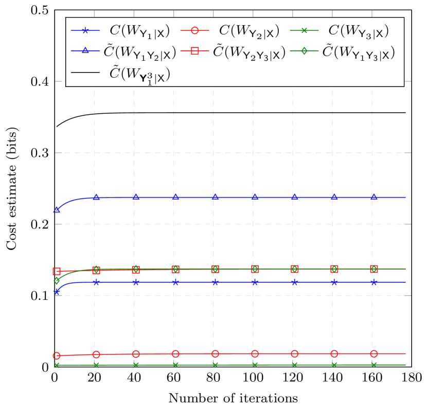
Figure 7: Convergence of the Blahut–Arimoto algorithm to the asymptotic simulation cost for the broadcast channel $W_{\mathbf{\mathsf{Y}}_{1}^{3}|X}=\mathrm{BSC}_{\mathsf{Y}_{3}|\mathsf{Y}_{2}}\circ\mathrm{BSC}_{\mathsf{Y}_{2}|\mathsf{Y}_{1}}\circ\mathrm{BSC}_{\mathsf{Y}_{1}|\mathsf{X}}$, where $\mathrm{BSC}$ refers to a binary symmetric channel with crossover probability $\delta=0.3$. The iterative procedure stops when increments for all quantities are smaller than $10^{-6}$ bits.

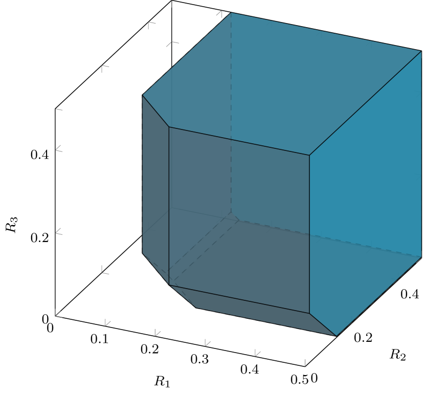
Figure 8: Asymptotic simulation region for the broadcast channel $W_{\mathbf{\mathsf{Y}}_{1}^{3}|\mathsf{X}}=\mathrm{BSC}_{\mathsf{Y}_{3}|\mathsf{Y}_{2}}\circ\mathrm{BSC}_{\mathsf{Y}_{2}|\mathsf{Y}_{1}}\circ\mathrm{BSC}_{\mathsf{Y}_{1}|\mathsf{X}}$, where $\mathrm{BSC}$ refers to a binary symmetric channel with crossover probability $\delta=0.3$.

Here we consider a broadcast channel with three receivers. For binary random variables $\mathsf{X},\mathsf{Y_{1}},\mathsf{Y_{2}}$ and $\mathsf{Y_{3}}$, let $W_{\mathsf{Y_{1}Y_{2}Y_{3}}|\mathsf{X}}=\mathrm{BSC}_{\mathsf{Y_{3}}|\mathsf{Y_{2}}}\circ\mathrm{BSC}_{\mathsf{Y_{2}}|\mathsf{Y_{1}}}\circ\mathrm{BSC}_{\mathsf{Y_{1}}|\mathsf{X}}$, where $\mathrm{BSC}$ is a binary symmetric channel with crossover probability $\delta=0.3$. Figure 8 shows the Blahut–Arimoto algorithm converging to the mutual information and common information terms. Since the optimal input distribution is the uniform distribution, we start with the initial guess $p^{(0)}_{\mathsf{X}}=(0.3,0.7)$ in Figure 8 to demonstrate iterative convergence. Unlike in the other sections, we do not show the sum of rates bounds e.g., $C_{\mathsf{Y}|\mathsf{X}}+C_{\mathsf{Z}|\mathsf{X}}$. Figure 8 shows the simulation region.

V-D3 Binary Skew-Symmetric Channel

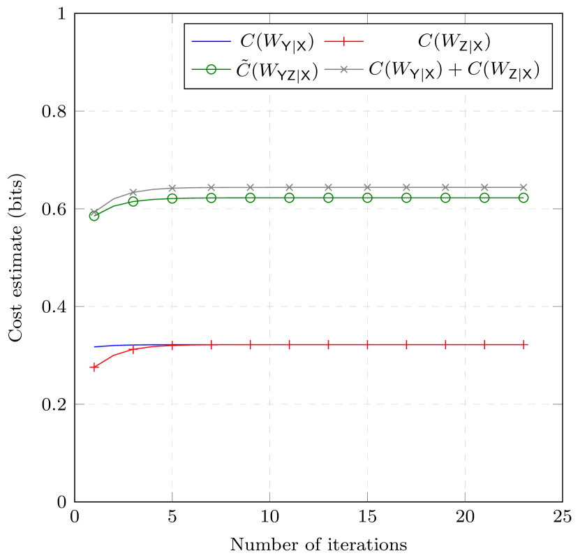
Figure 9: Convergence of the Blahut–Arimoto algorithm to the asymptotic simulation cost for the binary skew symmetric channel. The iterative procedure stops when increments for all quantities are smaller than $10^{-9}$ bits.

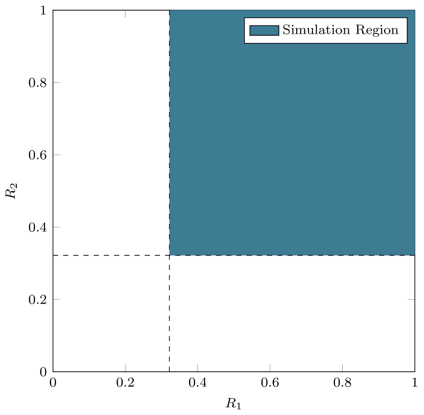
Figure 10: Asymptotic simulation region for the binary skew symmetric channel. Note that the bound due to $\widetilde{C}_{\mathsf{YZ}|\mathsf{X}}$ is redundant in this case.

The binary skew symmetric channel was studied in [47]. An expression for its capacity is unknown, despite some inner and outer bounds [48, 49]. In contrast, the asymptotic simulation cost is known exactly and we can compute it using the Blahut–Arimoto algorithm. The channel is given by the following conditional probability matrix

$$W_{\mathsf{YZ}|\mathsf{X}}=\begin{pmatrix}P_{00|0}&P_{00|1}\\ P_{01|0}&P_{01|1}\\ P_{10|0}&P_{10|1}\\ P_{11|0}&P_{11|1}\\ \end{pmatrix}=\begin{pmatrix}0.5&0\\ 0&0\\ 0.5&0.5\\ 0&0.5\\ \end{pmatrix}.$$ (216)

For this channel, it turns out that the bound regarding the common information is redundant and the mutual information bounds $C(W_{\mathsf{Y}|\mathsf{X}})=C(W_{\mathsf{Z}|\mathsf{X}})\approx 0.3219\text{ bits}$ determine the simulation region. Figures 10 and 10 show the Blahut–Arimoto algorithm converging to the asymptotic simulation cost and the simulation region respectively for this channel. Since the optimal input distribution for the common information is the uniform distribution, we start with the initial guess $p^{(0)}_{\mathsf{X}}=(0.3,0.7)$ to demonstrate iterative convergence in this figure.

VI Conclusions

In this work, we have introduced efficiently computable one-shot and finite blocklength bounds for the amount of communication needed for channel simulation. Second, we have used these bounds to derive tight higher order asymptotic expansions in the small and moderate deviation regime, and our results imply that channel interconversion becomes irreversible for finite blocklengths. Third, we have extended our results to network settings, where we have quantified the amount of communication needed for the simulation of $K$-receiver broadcast channels and have found an efficiently computable characterization of the rate region in terms of the multi-partite mutual information.

A potentially enlightening way to look at our results is through the lens of reversibility of channel interconversion. Both noisy channel coding and channel simulation can be seen as a special cases of the channel interconversion problem (see, e.g. [10] and references therein), where the task is to simulate a target channel $W$ using a resource channel $V$. It is then a fundamental question to characterize the asymptotics of the minimal rate, $\frac{m}{n}$, where $m$ is the number of uses of the resource channel required for the faithful simulation of $n$ instances of the target channel, i.e., to determine the capacity $C(V\mapsto W)$ of one channel $V$ to simulate another channel $W$.

For point-to-point discrete memoryless channels (DMCs), the special case of the identity channel $W=\operatorname{id}$ corresponds to Shannon’s noisy channel coding theorem, which gives a characterization of the channel capacity $C(V\mapsto\operatorname{id})=C(V)$ in terms of the mutual information of the channel $V$. This neat formula equally applies for worst and average case error criteria, as well as under additional assistance such as common randomness and feedback [50], or even so-called no-signaling correlations [15].

Channel simulation is another special case of interest and corresponds to the reverse problem of simulating a point-to-point DMC $W$ from the perfect resource channel $\operatorname{id}$. It is characterized by the reverse Shannon theorem [2], which states that, for a worst case error criteria and under common randomness assistance, one has the same characterization $C(\operatorname{id}\mapsto W)=C(W)^{-1}$ in terms the mutual information of the channel $W$. Taking these two findings together, one finds that the capacity of one channel $V$ to simulate another channel $W$ under common randomness assistance takes the form $C(V\mapsto W)=C(V)\cdot C^{-1}(W)$. As such, channel interconversion becomes asymptotically reversible and remarkably only one parameter is needed to quantify the potency of point-to-point DMCs under common randomness assistance.

Our results now show that channel interconversion becomes irreversible when we include second-order contribution in the small deviation expansion, unless the channel divergence vanishes for both channels. Moreover, our results also imply that broadcast channel interconversion is not asymptotically reversible.

Appendix A Proof of Lemma 12

Proof.

When $f$ is the zero function, the statement holds trivially. Otherwise, we first consider the case when $f$ is strictly positive. In this case, we define a pmf on $\mathcal{X}$ as $p^{\star}(x)\coloneqq f(x)/\sum_{x}f(x)$. It is obvious that $\max_{x}\frac{f(x)}{p^{\star}(x)}=\sum_{x}f(x)$. Assume that there exists some other pmf $p\in\mathcal{P}(\mathcal{X})$ such that $\max_{x}\frac{f(x)}{p(x)}<\max_{x}\frac{f(x)}{p^{\star}(x)}=\sum_{x}f(x)$. Then it must hold that $p(x)>p^{\star}(x)$ for all $x\in\mathcal{X}$, which is impossible. Hence, $p^{\star}$ is a minimizer, and

$$\inf_{p\in\mathcal{P}(\mathcal{X})}\max_{x\in\mathcal{X}}\frac{f(x)}{p(x)}=\max_{x}\frac{f(x)}{p^{\star}(x)}=\sum_{x}f(x).$$ (217)

Now, consider the case when $f$ is zero for some (but not all) $x\in\mathcal{X}$. Denote $\mathcal{X}_{0}\coloneqq\{x\in\mathcal{X}|f(x)=0\}$. We define a sequence of pmfs as

$$p_{n}(x)\coloneqq\begin{cases}2^{-\frac{1}{n}}\cdot p^{\star}_{\mathsf{X}}(x)&\text{ if }f(x)>0\\ \frac{1-2^{-\frac{1}{n}}}{\left\lvert\mathcal{X}_{0}\right\rvert}&\text{ otherwise.}\end{cases}$$ (218)

In this case, we have

$$\max_{x\in\mathcal{X}}\frac{f(x)}{p_{n}(x)}=2^{\frac{1}{n}}\cdot\sum_{x\in\mathcal{X}}f(x),$$ (219)

which is monotonically decreasing, and tends to $\sum_{x\in\mathcal{X}}f(x)$. This shows that

$$\inf_{p\in\mathcal{P}(\mathcal{X})}\max_{x\in\mathcal{X}}\frac{f(x)}{p(x)}\leqslant\sum_{x\in\mathcal{X}}f(x).$$ (220)

On the other hand , assume that there exists some pmf $p\in\mathcal{P}(\mathcal{X})$ such that $\max_{x}\frac{f(x)}{p(x)}<\sum_{x}f(x)$. Then, it must hold that $\frac{f(x)}{p(x)}<2^{\frac{1}{n}}\cdot\sum_{x\in\mathcal{X}}f(x)=\frac{f(x)}{p_{n}(x)}$ for all $x\in\mathcal{X}\setminus\mathcal{X}_{0}$ for all $n$, i.e., $p(x)>p_{n}(x)$ for all $x\in\mathcal{X}\setminus\mathcal{X}_{0}$ for all $n$. This implies that $p(x)\geqslant\lim_{n\to\infty}p_{n}(x)=p^{\star}(x)$ for all $x\in\mathcal{X}\setminus\mathcal{X}_{0}$. Since $p^{\star}(x)=0$ for $x\in\mathcal{X}_{0}$, it also holds that $p(x)\geqslant p^{\star}(x)$ for all $x\in\mathcal{X}_{0}$, and thus $p=p^{\star}$, which contradicts with the assumption that $\max_{x}\frac{f(x)}{p(x)}<\sum_{x}f(x)$. Hence,

$$\inf_{p\in\mathcal{P}(\mathcal{X})}\max_{x\in\mathcal{X}}\frac{f(x)}{p(x)}\geqslant\sum_{x\in\mathcal{X}}f(x),$$ (221)

which finishes the proof. ∎

Appendix B Proof of Lemma 13 in the case when $K=2$

In the case when $K=2$, Lemma 13 is stated as follows.

Lemma 20 (Bipartite Convex Split Lemma [23, Fact 7, modified]).

Let $\epsilon,\delta_{1},\delta_{2},\delta_{3}\in(0,1)$, such that $\delta_{1}^{2}+\delta_{2}^{2}+\delta_{3}^{2}\leqslant\epsilon^{2}$. Let $(\mathsf{X},\mathsf{Y},\mathsf{Z})$ be jointly distributed over $\mathcal{X}\times\mathcal{Y}\times\mathcal{Z}$ with pmf $p_{\mathsf{XYZ}}$. Let $q_{\mathsf{Y}}$ and $r_{\mathsf{Z}}$ be two pmfs over $\mathcal{Y}$ and $\mathcal{Z}$, respectively. Let $M$ and $N$ be two positive integers such that

$$\log{M} \geqslant D_{s+}^{\epsilon_{1}}\left(p_{\mathsf{XY}}\middle\|p_{\mathsf{X}}\times q_{\mathsf{Y}}\right)-\log{\delta_{1}^{2}},$$ (222)

$$\log{N} \geqslant D_{s+}^{\epsilon_{2}}\left(p_{\mathsf{XZ}}\middle\|p_{\mathsf{X}}\times r_{\mathsf{Z}}\right)-\log{\delta_{2}^{2}},$$ (223)

$$\log{M}+\log{N} \geqslant D_{s+}^{\epsilon_{3}}\left(p_{\mathsf{XYZ}}\middle\|p_{\mathsf{X}}\times q_{\mathsf{Y}}\times r_{\mathsf{Z}}\right)-\log{\delta_{3}^{2}},$$ (224)

for some $\epsilon_{1},\epsilon_{2},\epsilon_{3}\in(0,1)$ such that $\epsilon_{1}+\epsilon_{2}+\epsilon_{3}\leqslant\epsilon-\sqrt{\delta_{1}^{2}+\delta_{2}^{2}+\delta_{2}^{3}}$. Let $\mathsf{J}$ and $\mathsf{K}$ be independently uniformly distributed on $\{1,\ldots,M\}$ and $\{1,\ldots,N\}$, respectively. Let joint random variables $(\mathsf{J},\mathsf{K},\mathsf{X},\mathsf{Y}_{1},\ldots,\mathsf{Y}_{M},\mathsf{Z}_{1},\ldots,\mathsf{Z}_{N})$ be distributed according to

$$p_{\mathsf{X},\mathsf{Y}_{1},\ldots,\mathsf{Y}_{M},\mathsf{Z}_{1},\ldots,\mathsf{Z}_{N}|\mathsf{J},\mathsf{K}}(x,y_{1},\ldots,y_{M},z_{1},\ldots,z_{N}|j,k)=p_{\mathsf{XYZ}}(x,y_{j},z_{k})\cdot\prod_{i\neq j}q_{\mathsf{Y}}(y_{i})\cdot\prod_{\ell\neq k}r_{\mathsf{Z}}(z_{\ell}).$$ (225)

Then,

$$\left\lVert p_{\mathsf{X},\mathsf{Y}_{1},\ldots,\mathsf{Y}_{M},\mathsf{Z}_{1},\ldots,\mathsf{Z}_{N}}-p_{\mathsf{X}}\times q_{\mathsf{Y}_{1}}\times\cdots\times q_{\mathsf{Y}_{M}}\times r_{\mathsf{Z}_{1}}\times\cdots\times r_{\mathsf{Z}_{N}}\right\rVert_{\mathrm{tvd}}\leqslant\epsilon.$$ (226)

In the following, we provide a proof to the Lemma above. Note that the following proof is almost identical to the proof for [23, Fact 7], and is included here mainly for completeness. In addition, note that this proof can be generalized rather straightforwardly to the case when $K>2$.

Proof.

Define the subset $\mathcal{A}\subset\mathcal{X}\times\mathcal{Y}\times\mathcal{Z}$ as

$$\mathcal{A}\coloneqq\left\{(x,y,z)\middle|\begin{aligned} \frac{p_{\mathsf{XY}}(x,y)}{p_{\mathsf{X}}(x)\cdot q_{\mathsf{Y}}(y)}&\leqslant\delta_{1}^{2}\cdot M\\ \frac{p_{\mathsf{XYZ}}(x,z)}{p_{\mathsf{X}}(x)\cdot r_{\mathsf{Z}}(z)}&\leqslant\delta_{2}^{2}\cdot N\\ \frac{p_{\mathsf{XYZ}}(x,y,z)}{p_{\mathsf{X}}(x)\cdot q_{\mathsf{Y}}(y)\cdot r_{\mathsf{Z}}(z)}&\leqslant\delta_{3}^{2}\cdot MN\end{aligned}\right\}.$$ (227)

In this case,

$$p_{\mathsf{XYZ}}(\mathcal{A}^{C}) \leqslant\Pr\left[\frac{p_{\mathsf{XY}}(\mathsf{X},\mathsf{Y})}{p_{\mathsf{X}}(\mathsf{X})\cdot q_{\mathsf{Y}}(\mathsf{Y})}>\delta_{1}^{2}\!\cdot\!M\right] +\Pr\left[\frac{p_{\mathsf{XZ}}(\mathsf{X},\mathsf{Z})}{p_{\mathsf{X}}(\mathsf{X})\cdot r_{\mathsf{Z}}(\mathsf{Z})}>\delta_{2}^{2}\!\cdot\!N\right]+\Pr\left[\frac{p_{\mathsf{XYZ}}(\mathsf{X},\mathsf{Y},\mathsf{Z})}{p_{\mathsf{X}}(\mathsf{X})\cdot q_{\mathsf{Y}}(\mathsf{Y})\cdot r_{\mathsf{Z}}(\mathsf{Z})}>\delta_{3}^{2}\!\cdot\!MN\right]$$ (228)

$$\leqslant\epsilon_{1}+\epsilon_{2}+\epsilon_{3}\leqslant\epsilon-\delta,$$ (229)

where $\mathsf{XYZ}\sim p_{\mathsf{XYZ}}$ and $\delta\coloneqq\sqrt{\delta_{1}^{2}+\delta_{2}^{2}+\delta_{3}^{2}}$.

For each $x\in\mathcal{X}$, define $\mathcal{A}_{x}\coloneqq\{(y,z)\in\mathcal{Y}\times\mathcal{Z}:(x,y,z)\in\mathcal{A}\}$. Denote $\epsilon_{x}\coloneqq p_{\mathsf{YZ}|\mathsf{X}=x}(\mathcal{A}_{x}^{C})$. Then, $\sum_{x}\epsilon_{x}\cdot p_{\mathsf{X}}(x)=p_{\mathsf{XYZ}}(\mathcal{A}^{C})\leqslant\epsilon-\delta$. Let the random variables $(\mathsf{X}^{\prime},\mathsf{Y}^{\prime},\mathsf{Z}^{\prime})$ be distributed as $p_{\mathsf{X}^{\prime}\mathsf{Y}^{\prime}\mathsf{Z}^{\prime}}(x,y,z)=p_{\mathsf{X}}(x)\cdot p_{\mathsf{Y}^{\prime}\mathsf{Z}^{\prime}|\mathsf{X}^{\prime}}(y,z|x)$ where $p_{\mathsf{Y}^{\prime}\mathsf{Z}^{\prime}|\mathsf{X}^{\prime}}$ is defined as

$$p_{\mathsf{Y}^{\prime}\mathsf{Z}^{\prime}|\mathsf{X}^{\prime}}(y,z|x)\coloneqq\begin{cases}p_{\mathsf{YZ}|\mathsf{X}}(y,z|x)+\epsilon_{x}\cdot q_{\mathsf{Y}}(y)\cdot r_{\mathsf{Z}}(z)&\forall(y,z)\in\mathcal{A}_{x}\\ \epsilon_{x}\cdot q_{\mathsf{Y}}(y)\cdot r_{\mathsf{Z}}(z)&\text{otherwise}\end{cases}.$$ (230)

This distribution is $(\epsilon-\delta)$-close to the distribution of $(\mathsf{X},\mathsf{Y},\mathsf{Z})$ as

$$\left\lVert p_{\mathsf{XYZ}}-p_{\mathsf{X}^{\prime}\mathsf{Y}^{\prime}\mathsf{Z}^{\prime}}\right\rVert_{\mathrm{tvd}}= \sum_{x\in\mathcal{X}}p_{\mathsf{X}}(x)\cdot\left\lVert p_{\mathsf{YZ}|\mathsf{X}=x}-p_{\mathsf{Y}^{\prime}\mathsf{Z}^{\prime}|\mathsf{X}^{\prime}=x}\right\rVert_{\mathrm{tvd}}$$ (231)

$$\leqslant \frac{1}{2}\sum_{x\in\mathcal{X}}p_{\mathsf{X}}(x)\cdot\left(\sum_{(y,z)\in\mathcal{Y}\times\mathcal{Z}}\epsilon_{x}\cdot q_{\mathsf{Y}}(y)\cdot r_{\mathsf{Z}}(z)+\sum_{(y,z)\not\in\mathcal{A}_{x}}p_{\mathsf{YZ}|\mathsf{X}}(y,z|x)\right)$$ (232)

$$= \frac{1}{2}\cdot\sum_{x\in\mathcal{X}}p_{\mathsf{X}}(x)\cdot\left(\epsilon_{x}+p_{\mathsf{YZ}|\mathsf{X}=x}(\mathcal{A}_{x}^{C})\right)=p_{\mathsf{XYZ}}(\mathcal{A}^{C})\leqslant\epsilon-\delta.$$ (233)

Additionally, by the definitions of $\{\mathcal{A}_{x}\}_{x\in\mathcal{X}}$ and $\mathcal{A}$, we have (notice that $M\cdot N\geqslant 1/\delta_{3}^{2}$ due to (224))

$$p_{\mathsf{Y}^{\prime}\mathsf{Z}^{\prime}|\mathsf{X}^{\prime}}(y,z|x) \leqslant(\delta_{3}^{2}\cdot MN+\epsilon_{x})\cdot q_{\mathsf{Y}}(y)\cdot r_{\mathsf{Z}}(z)$$ (234)

$$\leqslant(\delta_{3}^{2}\cdot MN+1)\cdot q_{\mathsf{Y}}(y)\cdot r_{\mathsf{Z}}(z)$$ (235)

$$\leqslant 2\delta_{3}^{2}\cdot MN\cdot q_{\mathsf{Y}}(y)\cdot r_{\mathsf{Z}}(z).$$ (236)

Similarly, we have

$$p_{\mathsf{Y}^{\prime}|\mathsf{X}^{\prime}}(y|x) \leqslant 2\delta_{1}^{2}\cdot M\cdot q_{\mathsf{Y}}(y),$$ (237)

$$p_{\mathsf{Z}^{\prime}|\mathsf{X}^{\prime}}(z|x) \leqslant 2\delta_{3}^{2}\cdot N\cdot r_{\mathsf{Z}}(z).$$ (238)

Now, construct $(\mathsf{X}^{\prime},\mathsf{Y}^{\prime}_{1},\ldots,\mathsf{Y}^{\prime}_{M},\mathsf{Z}^{\prime}_{1},\ldots,\mathsf{Z}^{\prime}_{N})$ from $(\mathsf{X}^{\prime},\mathsf{Y}^{\prime},\mathsf{Z}^{\prime})$ in the same fashion as the construction of $(\mathsf{X},\mathsf{Y}_{1},\ldots,\mathsf{Y}_{M}$, $\mathsf{Z}_{1},\ldots,\mathsf{Z}_{N})$ from $(\mathsf{X},\mathsf{Y},\mathsf{Z})$. We have

$$\left\lVert p_{\mathsf{X}^{\prime},\mathsf{Y}^{\prime}_{1},\ldots,\mathsf{Y}^{\prime}_{M},\mathsf{Z}^{\prime}_{1},\ldots,\mathsf{Z}^{\prime}_{N}}-p_{\mathsf{X},\mathsf{Y}_{1},\ldots,\mathsf{Y}_{M},\mathsf{Z}_{1},\ldots,\mathsf{Z}_{N}}\right\rVert_{\mathrm{tvd}}\leqslant\left\lVert p_{\mathsf{XYZ}}-p_{\mathsf{X}^{\prime}\mathsf{Y}^{\prime}\mathsf{Z}^{\prime}}\right\rVert_{\mathrm{tvd}}\leqslant\epsilon-\delta,$$ (239)

and

$$\phantom{=}D\left(p_{\mathsf{X}^{\prime},\mathsf{Y}^{\prime}_{1},\ldots,\mathsf{Y}^{\prime}_{M},\mathsf{Z}^{\prime}_{1},\ldots,\mathsf{Z}^{\prime}_{N}}\middle\|p_{\mathsf{X}^{\prime}}\times\prod_{i=1}^{M}q_{\mathsf{Y}^{\prime}_{i}}\times\prod_{\ell=1}^{N}r_{\mathsf{Z}^{\prime}_{\ell}}\right)$$

$$=\frac{1}{MN}\sum_{j,k}\left\{D\left(p_{\mathsf{X}^{\prime}\mathsf{Y}^{\prime}_{j}\mathsf{Z}^{\prime}_{k}}\middle\|p_{\mathsf{X}^{\prime}}\times q_{\mathsf{Y}^{\prime}_{j}}\times r_{\mathsf{Z}^{\prime}_{k}}\right)-D\left(p_{\mathsf{X}^{\prime}\mathsf{Y}^{\prime}_{j}\mathsf{Z}^{\prime}_{k}}\times\prod_{i\neq j}q_{\mathsf{Y}^{\prime}_{i}}\times\prod_{\ell\neq k}r_{\mathsf{Z}^{\prime}_{\ell}}\middle\|p_{\mathsf{X}^{\prime},\mathsf{Y}^{\prime}_{1},\ldots,\mathsf{Y}^{\prime}_{M},\mathsf{Z}^{\prime}_{1},\ldots,\mathsf{Z}^{\prime}_{N}}\right)\right\}$$ (240)

$$\leqslant\begin{aligned} &D\left(p_{\mathsf{X}^{\prime}\mathsf{Y}^{\prime}\mathsf{Z}^{\prime}}\middle\|p_{\mathsf{X}^{\prime}}\times q_{\mathsf{Y}^{\prime}}\times r_{\mathsf{Z}^{\prime}}\right)-\\ &D\left(p_{\mathsf{X}^{\prime}\mathsf{Y}^{\prime}\mathsf{Z}^{\prime}}\middle\|\frac{1}{MN}p_{\mathsf{X}^{\prime}\mathsf{Y}^{\prime}\mathsf{Z}^{\prime}}+\frac{N-1}{MN}p_{\mathsf{X}^{\prime}\mathsf{Y}^{\prime}}\times r_{\mathsf{Z}^{\prime}}+\frac{M-1}{MN}p_{\mathsf{X}^{\prime}\mathsf{Z}^{\prime}}\times q_{\mathsf{Y}^{\prime}}+\frac{(M-1)(N-1)}{MN}p_{\mathsf{X}^{\prime}}\times q_{\mathsf{Y}^{\prime}}\times r_{\mathsf{Z}^{\prime}}\right)\end{aligned}$$ (241)

$$=\sum_{x,y,z}p_{\mathsf{X}^{\prime}\mathsf{Y}^{\prime}\mathsf{Z}^{\prime}}(x,y,z)\cdot\log\left(\frac{1}{MN}\cdot\frac{p_{\mathsf{Y}^{\prime}\mathsf{Z}^{\prime}|\mathsf{X}^{\prime}}(y,z|x)}{q_{\mathsf{Y}}(y)\cdot r_{\mathsf{Z}}(z)}+\frac{N\!-\!1}{MN}\cdot\frac{p_{\mathsf{Y}^{\prime}|\mathsf{X}^{\prime}}(y|x)}{q_{\mathsf{Y}}(y)}+\frac{M\!-\!1}{MN}\cdot\frac{p_{\mathsf{Z}^{\prime}|\mathsf{X}^{\prime}}(z|x)}{r_{\mathsf{Z}}(z)}+\frac{(M\!-\!1)(N\!-\!1)}{MN}\right)$$ (242)

$$\leqslant\log\left(1+2\delta_{1}^{2}+2\delta_{2}^{2}+2\delta_{3}^{2}\right)\leqslant 2\delta^{2},$$ (243)

which, by Pinsker’s inequality, implies that

$$\left\lVert p_{\mathsf{X}^{\prime},\mathsf{Y}^{\prime}_{1},\ldots,\mathsf{Y}^{\prime}_{M},\mathsf{Z}^{\prime}_{1},\ldots,\mathsf{Z}^{\prime}_{N}}-p_{\mathsf{X}^{\prime}}\times\prod_{i=1}^{M}q_{\mathsf{Y}^{\prime}_{i}}\times\prod_{\ell=1}^{N}r_{\mathsf{Z}^{\prime}_{\ell}}\right\rVert_{\mathrm{tvd}}\leqslant\delta.$$ (244)

Finally, to show (226), one applies triangular inequality while noticing that $p_{\mathsf{X}^{\prime}}=p_{\mathsf{X}}$. ∎

Appendix C Proof of Blahut-Arimoto Results

C-A Extension Function and Update Rule

This section uses the framework from [52]. Recall that we are interested in solving the following optimization problem

$$\max_{p_{\mathsf{X}}\in\mathcal{P}(\mathcal{X})}I(\mathsf{X}:\mathsf{Y_{1}}:\mathsf{Y_{2}}:\cdots:\mathsf{Y_{K}})_{p_{\mathsf{X}}\cdot W_{\mathbf{\mathsf{Y}}_{1}^{K}|\mathsf{X}}}.$$ (245)

The method is to maximize the following bi-variate function (known as the extension function) alternatively until it converges to $\widetilde{C}(W)$:

$$J(p_{\mathsf{X}},q_{\mathsf{X}}) \coloneqq I(\mathsf{X}:\mathsf{Y_{1}}:\mathsf{Y_{2}}:\cdots:\mathsf{Y_{K}})_{p_{\mathsf{X}}\cdot W_{\mathbf{\mathsf{Y}}_{1}^{K}|\mathsf{X}}}+\sum_{i=1}^{K}D\left(p_{\mathsf{Y}_{i}}\middle\|q_{\mathsf{Y}_{i}}\right)-K\cdot D\left(p_{\mathsf{X}}\middle\|q_{\mathsf{X}}\right)$$ (246)

$$=-K\cdot D\left(p_{\mathsf{X}}\middle\|q_{\mathsf{X}}\right)+\sum_{x\in\mathcal{X}}p_{\mathsf{X}}(x)\cdot D\left(W_{\mathbf{\mathsf{Y}}_{1}^{K}|\mathsf{X}}(\cdot|x)\middle\|q_{\mathsf{Y}_{1}}\times\cdots\times q_{\mathsf{Y}_{K}}\right)$$ (247)

$$=\sum_{x\in\mathcal{X}}p_{\mathsf{X}}(x)\left[-K\cdot\log{p_{\mathsf{X}}(x)}+K\cdot\log{q_{\mathsf{X}}(x)}+D\left(W_{\mathbf{\mathsf{Y}}_{1}^{K}|\mathsf{X}}(\cdot|x)\middle\|q_{\mathsf{Y}_{1}}\times\cdots\times q_{\mathsf{Y}_{K}}\right)\right],$$ (248)

where $p_{\mathsf{Y}_{i}}(\cdot)\coloneqq\sum_{x\in\mathcal{X}}W_{\mathsf{Y}_{i}|\mathsf{X}}(\cdot|x)\cdot p_{\mathsf{X}}(x)$ and $q_{\mathsf{Y}_{i}}(\cdot)\coloneqq\sum_{x\in\mathcal{X}}W_{\mathsf{Y}_{i}|\mathsf{X}}(\cdot|x)\cdot q_{\mathsf{X}}(x)$. On the one hand, it is clear that

$$\operatorname{argmax}_{q_{\mathsf{X}}\in\mathcal{P}(\mathcal{X})}J(p_{\mathsf{X}},q_{\mathsf{X}})=p_{\mathsf{X}}$$ (249)

due to the data processing inequality. On the other hand, for each $q_{\mathsf{X}}\in\mathcal{P}(\mathcal{X})$, the funciton $J(p_{\mathsf{X}},q_{\mathsf{X}})$ is concave in $p_{\mathsf{X}}$. Thus, by requiring the partial derivative of $J$ with respect to $p_{\mathsf{X}}$ to be $0$, we find the optimal $p_{\mathsf{X}}$ to be

$$p_{\mathsf{X}}\propto q_{\mathsf{X}}\cdot\exp{\left(\frac{D\left(W_{\mathbf{\mathsf{Y}}_{1}^{K}|\mathsf{X}}(\cdot|x)\middle\|q_{\mathsf{Y}_{1}}\times\cdots\times q_{\mathsf{Y}_{K}}\right)}{K}\right)}.$$ (250)

Combining (249) and (250), we end up with the update rule as in (214).

C-B Speed of Convergence

At $n$-th step, we estimate the $K$-partite common information as

$$\widetilde{C}(n)\coloneqq J(p_{\mathsf{X}}^{(n)},p_{\mathsf{X}}^{(n\!-\!1)}) =\sum_{x\in\mathcal{X}}p^{(n)}_{\mathsf{X}}(x)\left[-K\!\cdot\!\log{p^{(n)}_{\mathsf{X}}(x)}+K\!\cdot\!\log{p^{(n\!-\!1)}_{\mathsf{X}}(x)}+D\left(W_{\mathbf{\mathsf{Y}}_{1}^{K}|\mathsf{X}}(\cdot|x)\middle\|p^{(n\!-\!1)}_{\mathsf{Y}_{1}}\times\cdots\times p^{(n\!-\!1)}_{\mathsf{Y}_{K}}\right)\right]$$ (251)

$$=\sum_{x\in\mathcal{X}}p^{(n)}_{\mathsf{X}}(x)\cdot K\cdot\log{\left(\sum_{\widetilde{x}}p^{(n-1)}_{\mathsf{X}}(\widetilde{x})\cdot\exp{\left(\frac{D\left(W_{\mathbf{\mathsf{Y}}_{1}^{K}|\mathsf{X}}(\cdot|\widetilde{x})\middle\|p^{(n-1)}_{\mathsf{Y}_{1}}\times\cdots\times p^{(n-1)}_{\mathsf{Y}_{K}}\right)}{K}\right)}\right)}$$ (252)

$$=K\cdot\log{\left(\sum_{\widetilde{x}}p^{(n-1)}_{\mathsf{X}}(\widetilde{x})\cdot\exp{\left(\frac{D\left(W_{\mathbf{\mathsf{Y}}_{1}^{K}|\mathsf{X}}(\cdot|\widetilde{x})\middle\|p^{(n-1)}_{\mathsf{Y}_{1}}\times\cdots\times p^{(n-1)}_{\mathsf{Y}_{K}}\right)}{K}\right)}\right)},$$ (253)

where we have used the update rule (214) for $p_{\mathsf{X}}^{(n)}$. Let $p^{\operatorname{\raisebox{0.3pt}{\mbox{\tiny$\blacktriangle$}}}}_{\mathsf{X}}$ be a pmf achieving $\widetilde{C}(W)$. We have

$$\sum_{x\in\mathcal{X}}p^{\operatorname{\raisebox{0.3pt}{\mbox{\tiny$\blacktriangle$}}}}_{\mathsf{X}}(x)\cdot\left(\log{p_{\mathsf{X}}^{(n)}(x)}-\log{p_{\mathsf{X}}^{(n-1)}(x)}\right)$$

$$= \sum_{x\in\mathcal{X}}p^{\operatorname{\raisebox{0.3pt}{\mbox{\tiny$\blacktriangle$}}}}_{\mathsf{X}}(x)\cdot\begin{aligned} &\left(\frac{D\left(W_{\mathbf{\mathsf{Y}}_{1}^{K}|\mathsf{X}}(\cdot|x)\middle\|p^{(n-1)}_{\mathsf{Y}_{1}}\times\cdots\times p^{(n-1)}_{\mathsf{Y}_{K}}\right)}{K}\right.\\ &\hskip 107.0pt\left.-\log{\left(\sum_{\widetilde{x}}p^{(n-1)}_{\mathsf{X}}(\widetilde{x})\cdot\exp{\left(\frac{D\left(W_{\mathbf{\mathsf{Y}}_{1}^{K}|\mathsf{X}}(\cdot|\widetilde{x})\middle\|p^{(n-1)}_{\mathsf{Y}_{1}}\times\cdots\times p^{(n-1)}_{\mathsf{Y}_{K}}\right)}{K}\right)}\right)}\right)\end{aligned}$$ (254)

$$= -\frac{1}{K}\widetilde{C}(n)+\frac{1}{K}\begin{aligned} \Bigg{(}&\sum_{x\in\mathcal{X}}p^{\operatorname{\raisebox{0.3pt}{\mbox{\tiny$\blacktriangle$}}}}_{\mathsf{X}}(x)\cdot D\left(W_{\mathbf{\mathsf{Y}}_{1}^{K}|\mathsf{X}}(\cdot|x)\middle\|p^{(n-1)}_{\mathsf{Y}_{1}}\times\cdots\times p^{(n-1)}_{\mathsf{Y}_{K}}\right)\\ &\hskip 162.0pt+\sum_{i=1}^{K}\sum_{y}p^{\operatorname{\raisebox{0.3pt}{\mbox{\tiny$\blacktriangle$}}}}_{\mathsf{Y}_{i}}(y)\log{p^{\operatorname{\raisebox{0.3pt}{\mbox{\tiny$\blacktriangle$}}}}_{\mathsf{Y}_{i}}(y)}-\sum_{i=1}^{K}\sum_{y}p^{\operatorname{\raisebox{0.3pt}{\mbox{\tiny$\blacktriangle$}}}}_{\mathsf{Y}_{i}}(y)\log{p^{\operatorname{\raisebox{0.3pt}{\mbox{\tiny$\blacktriangle$}}}}_{\mathsf{Y}_{i}}(y)}\Bigg{)}\end{aligned}$$ (255)

$$= \frac{1}{K}\left(\widetilde{C}(W)-\widetilde{C}(n)+\sum_{i=1}^{K}D\left(p^{\operatorname{\raisebox{0.3pt}{\mbox{\tiny$\blacktriangle$}}}}_{\mathsf{Y}_{i}}\middle\|p^{(n-1)}_{\mathsf{Y}_{i}}\right)\right)$$ (256)

$$\geqslant \frac{1}{K}\left(\widetilde{C}(W)-\widetilde{C}(n)\right).$$ (257)

Choosing $p^{(0)}_{\mathsf{X}}$ to be the uniform distribution on $\mathcal{X}$, we have

$$\frac{1}{K}\sum_{i=1}^{n}\widetilde{C}(W)-\widetilde{C}(n) \leqslant\sum_{i=1}^{n}\sum_{x\in\mathcal{X}}p^{\operatorname{\raisebox{0.3pt}{\mbox{\tiny$\blacktriangle$}}}}_{\mathsf{X}}(x)\cdot\left(\log{p_{\mathsf{X}}^{(i)}(x)}-\log{p_{\mathsf{X}}^{(i-1)}(x)}\right)$$ (258)

$$=\sum_{x\in\mathcal{X}}p^{\operatorname{\raisebox{0.3pt}{\mbox{\tiny$\blacktriangle$}}}}_{\mathsf{X}}(x)\cdot\left(\log{p_{\mathsf{X}}^{(n)}(x)}-\log{p_{\mathsf{X}}^{(0)}(x)}\right)$$ (259)

$$=D\left(p^{\operatorname{\raisebox{0.3pt}{\mbox{\tiny$\blacktriangle$}}}}_{\mathsf{X}}\middle\|p_{\mathsf{X}}^{(0)}\right)-D\left(p^{\operatorname{\raisebox{0.3pt}{\mbox{\tiny$\blacktriangle$}}}}_{\mathsf{X}}\middle\|p_{\mathsf{X}}^{(n)}\right)$$ (260)

$$\leqslant D\left(p^{\operatorname{\raisebox{0.3pt}{\mbox{\tiny$\blacktriangle$}}}}_{\mathsf{X}}\middle\|p_{\mathsf{X}}^{(0)}\right)$$ (261)

$$\leqslant\log{\left\lvert\mathcal{X}\right\rvert}.$$ (262)

Note that $\widetilde{C}(n)$ is monotonically non-decreasing in $n$ and $\widetilde{C}(n)\leqslant\widetilde{C}(W)$ for all $n$. One must have

$$\left\lvert\widetilde{C}(W)-\widetilde{C}(n)\right\rvert\leqslant\frac{K}{n}\log{\left\lvert\mathcal{X}\right\rvert}.$$ (263)

Finally, we need to point out that the above discussion is a worst-case analysis and holds for all channels. In practice, the algorithm converges much faster.

References

- [1] M. X. Cao, N. Ramakrishnan, M. Berta, and M. Tomamichel, “One-shot point-to-point channel simulation,” in 2022 IEEE International Symposium on Information Theory (ISIT). IEEE, 2022, pp. 796–801.
- [2] C. H. Bennett, P. W. Shor, J. A. Smolin, and A. V. Thapliyal, “Entanglement-assisted capacity of a quantum channel and the reverse Shannon theorem,” IEEE Transactions on Information Theory, vol. 48, no. 10, pp. 2637–2655, 2002.
- [3] C. H. Bennett, I. Devetak, A. W. Harrow, P. W. Shor, and A. Winter, “The quantum reverse Shannon theorem and resource tradeoffs for simulating quantum channels,” IEEE Transactions on Information Theory, vol. 60, no. 5, pp. 2926–2959, 2014.
- [4] A. Wyner, “The common information of two dependent random variables,” IEEE Transactions on Information Theory, vol. 21, no. 2, pp. 163–179, 1975.
- [5] T. Han and S. Verdu, “Approximation theory of output statistics,” IEEE Transactions on Information Theory, vol. 39, no. 3, pp. 752–772, 1993.
- [6] P. W. Cuff, H. H. Permuter, and T. M. Cover, “Coordination capacity,” IEEE Transactions on Information Theory, vol. 56, no. 9, pp. 4181–4206, 2010.
- [7] P. Harsha, R. Jain, D. McAllester, and J. Radhakrishnan, “The communication complexity of correlation,” IEEE Transactions on Information Theory, vol. 56, no. 1, pp. 438–449, 2010.
- [8] P. Cuff, “Distributed channel synthesis,” IEEE Transactions on Information Theory, vol. 59, no. 11, pp. 7071–7096, 2013.
- [9] L. Yu and V. Y. Tan, “Exact channel synthesis,” IEEE Transactions on Information Theory, vol. 66, no. 5, pp. 2799–2818, 2019.
- [10] M. Sudan, H. Tyagi, and S. Watanabe, “Communication for generating correlation: A unifying survey,” IEEE Transactions on Information Theory, vol. 66, no. 1, pp. 5–37, 2020.
- [11] A. Anshu, M. Berta, R. Jain, and M. Tomamichel, “Partially smoothed information measures,” IEEE Transactions on Information Theory, vol. 66, no. 8, pp. 5022–5036, 2020.
- [12] K. Fang, X. Wang, M. Tomamichel, and M. Berta, “Quantum channel simulation and the channel’s smooth max-information,” IEEE Transactions on Information Theory, vol. 66, no. 4, pp. 2129–2140, 2019.
- [13] Y. Polyanskiy, H. V. Poor, and S. Verdú, “Channel coding rate in the finite blocklength regime,” IEEE Transactions on Information Theory, vol. 56, no. 5, pp. 2307–2359, 2010.
- [14] M. Hayashi, “Information spectrum approach to second-order coding rate in channel coding,” IEEE Transactions on Information Theory, vol. 55, no. 11, pp. 4947–4966, 2009.
- [15] W. Matthews, “A linear program for the finite block length converse of Polyanskiy–Poor–Verdú via nonsignaling codes,” IEEE Transactions on Information Theory, vol. 58, no. 12, pp. 7036–7044, 2012.
- [16] J. Von Neumann, “Various techniques used in connection with random digits,” in Monte Carlo Method, ser. National Bureau of Standards: Applied Mathematics Series, A. S. Householder, G. E. Forsythe, and H. H. Germond, Eds. United States Government Printing Office, 1951, vol. 12, ch. 13, pp. 36–38.
- [17] C. P. Robert, G. Casella, and G. Casella, Monte Carlo statistical methods. Springer, 1999, vol. 2.
- [18] R. Jain, J. Radhakrishnan, and P. Sen, “A direct sum theorem in communication complexity via message compression,” in International Colloquium on Automata, Languages, and Programming. Springer, 2003, pp. 300–315.
- [19] V. Strassen, “Asymptotic estimates in Shannon’s information theory [Asymptotische Abschätzungen in Shannon’s Informationstheorie],” in Transactions of the Third Prague Conference on Information Theory, Statistical Decision Functions, Random Processes. Prague: Czechoslovak Academy of Sciences, 1962, pp. 689–723.
- [20] Y. Polyanskiy and S. Verdú, “Channel dispersion and moderate deviations limits for memoryless channels,” in 2010 48th Annual Allerton Conference on Communication, Control, and Computing (Allerton). IEEE, 2010, pp. 1334–1339.
- [21] W. McGill, “Multivariate information transmission,” Transactions of the IRE Professional Group on Information Theory, vol. 4, no. 4, pp. 93–111, 1954.
- [22] S. Watanabe, “Information theoretical analysis of multivariate correlation,” IBM Journal of Research and Development, vol. 4, no. 1, pp. 66–82, 1960.
- [23] A. Anshu, R. Jain, and N. A. Warsi, “A unified approach to source and message compression,” arXiv preprint arXiv:1707.03619, 2017.
- [24] A. Anshu, V. K. Devabathini, and R. Jain, “Quantum communication using coherent rejection sampling,” Physical Review Letters, vol. 119, no. 12, p. 120506, 2017.
- [25] T. Cover, “Comments on broadcast channels,” IEEE Transactions on Information Theory, vol. 44, no. 6, pp. 2524–2530, 1998.
- [26] L. Yu and V. Y. F. Tan, “Common information, noise stability, and their extensions,” Foundations and Trends® in Communications and Information Theory, vol. 19, no. 2, pp. 107–389, 2022.
- [27] ——, “On exact and -Rényi common informations,” IEEE Transactions on Information Theory, vol. 66, no. 6, pp. 3366–3406, 2020.
- [28] C. T. Li and A. E. Gamal, “Strong functional representation lemma and applications to coding theorems,” IEEE Transactions on Information Theory, vol. 64, no. 11, pp. 6967–6978, 2018.
- [29] A. Winter, “Compression of sources of probability distributions and density operators,” arXiv preprint arXiv:quant-ph/0208131, 2002.
- [30] M. H. Yassaee, A. Gohari, and M. R. Aref, “Channel simulation via interactive communications,” IEEE Transactions on Information Theory, vol. 61, no. 6, pp. 2964–2982, 2015.
- [31] P. Cuff, “Communication in networks for coordinating behavior,” Ph.D. dissertation, Stanford University, 2009.
- [32] F. Haddadpour, M. H. Yassaee, S. Beigi, A. Gohari, and M. R. Aref, “Simulation of a channel with another channel,” IEEE Transactions on Information Theory, vol. 63, no. 5, pp. 2659–2677, 2016.
- [33] G. R. Kurri, V. Ramachandran, S. R. B. Pillai, and V. M. Prabhakaran, “Multiple access channel simulation,” IEEE Transactions on Information Theory, pp. 1–1, 2022.
- [34] M. Berta, M. Christandl, and R. Renner, “The quantum reverse Shannon theorem based on one-shot information theory,” Communications in Mathematical Physics, vol. 306, no. 3, pp. 579–615, 2011.
- [35] M. Berta, J. M. Renes, and M. M. Wilde, “Identifying the information gain of a quantum measurement,” IEEE Transactions on Information Theory, vol. 60, no. 12, pp. 7987–8006, 2014.
- [36] N. Ramakrishnan, M. Tomamichel, and M. Berta, “Moderate deviation expansion for fully quantum tasks,” IEEE Transactions on Information Theory, 2023.
- [37] M. Christandl, R. König, and R. Renner, “Postselection technique for quantum channels with applications to quantum cryptography,” Physical Review Letters, vol. 102, no. 2, p. 020504, 2009.
- [38] M. Hayashi, “Universal coding for classical-quantum channel,” Communications in Mathematical Physics, vol. 289, no. 3, pp. 1087–1098, 2009.
- [39] M. Berta, “Quantum side information: Uncertainty relations, extractors, channel simulations,” arXiv preprint arXiv:1310.4581, 2013.
- [40] M. Tomamichel and M. Hayashi, “A hierarchy of information quantities for finite block length analysis of quantum tasks,” IEEE Transactions on Information Theory, vol. 59, no. 11, pp. 7693–7710, 2013.
- [41] Y. Polyanskiy, “Saddle point in the minimax converse for channel coding,” IEEE Transactions on Information Theory, vol. 59, no. 5, pp. 2576–2595, 2012.
- [42] T. S. Cubitt, D. Leung, W. Matthews, and A. Winter, “Zero-error channel capacity and simulation assisted by non-local correlations,” IEEE Transactions on Information Theory, vol. 57, no. 8, pp. 5509–5523, 2011.
- [43] M. Tomamichel and V. Y. Tan, “A tight upper bound for the third-order asymptotics for most discrete memoryless channels,” IEEE Transactions on Information Theory, vol. 59, no. 11, pp. 7041–7051, 2013.
- [44] S. Verdú et al., “A general formula for channel capacity,” IEEE Transactions on Information Theory, vol. 40, no. 4, pp. 1147–1157, 1994.
- [45] R. Blahut, “Computation of channel capacity and rate-distortion functions,” IEEE transactions on Information Theory, vol. 18, no. 4, pp. 460–473, 1972.
- [46] S. Arimoto, “An algorithm for computing the capacity of arbitrary discrete memoryless channels,” IEEE Transactions on Information Theory, vol. 18, no. 1, pp. 14–20, 1972.
- [47] B. Hajek and M. Pursley, “Evaluation of an achievable rate region for the broadcast channel,” IEEE Transactions on Information Theory, vol. 25, no. 1, pp. 36–46, 1979.
- [48] K. Marton, “A coding theorem for the discrete memoryless broadcast channel,” IEEE Transactions on Information Theory, vol. 25, no. 3, pp. 306–311, 1979.
- [49] C. Nair and A. El Gamal, “An outer bound to the capacity region of the broadcast channel,” IEEE Transactions on Information Theory, vol. 53, no. 1, pp. 350–355, 2006.
- [50] C. Shannon, “The zero error capacity of a noisy channel,” IRE Transactions on Information Theory, vol. 2, no. 3, pp. 8–19, 1956.
- [51] P. Hayden and F. Dupuis, “A reverse Shannon theorem for quantum broadcast channels,” 2007, CMS-MITACS Joint Conference.
- [52] N. Ramakrishnan, R. Iten, V. B. Scholz, and M. Berta, “Computing quantum channel capacities,” IEEE Transactions on Information Theory, vol. 67, no. 2, pp. 946–960, 2020.