December 22, 2022

Precision calculations of $B_{d,s}\to\pi,K$ decay form factors
in soft-collinear effective theory

Bo-Yan Cui^a, Yong-Kang Huang^a , Yue-Long Shen^b, Chao Wang^c, Yu-Ming Wang^a
a   School of Physics, Nankai University, Weijin Road 94, 300071 Tianjin, China

^b College of Information Science and Engineering, Ocean University of China,
Qingdao 266100, Shandong, China

^c College of Mathematics and Physics, Huaiyin Institute of Technology,
Huaian 223003, Jiangsu, China

We improve QCD calculations of the semileptonic $B_{d,s}\to\pi,K$ decay form factors at large hadronic recoil by implementing the next-to-leading-logarithmic resummation for the obtained leading-power light-cone sum rules in the soft-collinear effective theory (SCET) framework and by computing for the first time the non-vanishing spectator-quark mass correction dictating the SU(3)-flavour symmetry breaking effects between these fundamental quantities at the one-loop accuracy. Additionally, we endeavour to investigate a variety of the subleading-power contributions to these heavy-to-light form factors at ${\cal O}(\alpha_{s}^{0})$ with the same methodology, by including the higher-order terms in the heavy-quark expansion of the hard-collinear quark propagator, by evaluating the desired effective matrix element of the next-to-leading-order term $(\bar{\xi}_{\rm hc}\,W_{\rm hc})\,\gamma_{\mu}\,\left[i\,{\not{D}}_{\top}/\left(2\,m_{b}\right)\right]\,h_{v}$ in the ${\rm SCET_{I}}$ representation of the weak transition current, by taking into account the off-light-cone contributions of the two-body heavy-quark effective theory (HQET) matrix elements as well as the three-particle higher-twist corrections from the subleading bottom-meson light-cone distribution amplitudes (LCDAs), and by computing the twist-five and twist-six four-body higher-twist effects with the aid of the factorization approximation. Having at our disposal the SCET sum rules for the exclusive $B$-meson decay form factors under discussion, we further explore in detail numerical implications of the newly computed subleading-power corrections by employing the three-parameter model for both the leading-twist and higher-twist $B$-meson distribution amplitudes. Taking advantage of the customary Bourrely-Caprini-Lellouch (BCL) parametrization for the complete set of the semileptonic $B_{d,s}\to\pi,K$ form factors, we then determine the correlated numerical results for the interesting series coefficients, by carrying out the simultaneous fit of the exclusive $B$-meson decay form factors to both the achieved SCET sum rule predictions at small momentum transfer ($q^{2}$) and the available lattice QCD results at large momentum transfer. Subsequently, we perform a comprehensive phenomenological analysis of the full angular observables, the lepton-flavour university ratios and the lepton polarization asymmetries for the flavour-changing charged-current $B\to\pi\ell\bar{\nu}_{\ell}$ and $B_{s}\to K\ell\bar{\nu}_{\ell}$ decays (with $\ell=\mu,\,\tau$) together with the differential $q^{2}$-distribution for the exclusive rare $B\to K\nu_{\ell}\bar{\nu}_{\ell}$ decays in the Standard Model.

1 Introduction

Precision calculations of the semileptonic $B_{d,s}\to\pi,K$ decay form factors are of paramount importance for exploring the celebrated Cabibbo-Kobayashi-Maskawa (CKM) mechanism in the Standard Model (SM) and for sharpening our understanding towards diverse facets of the strong interaction dynamics encoded in the exclusive heavy-hadron decay processes. Particularly, the longstanding discrepancy between the dedicated $|V_{ub}|$ determinations from the exclusive $B\to\pi\ell\bar{\nu}_{\ell}$ decays and the inclusive $B\to X_{u}\ell\bar{\nu}_{\ell}$ processes [1] has been continually triggering the enormous theoretical efforts of determining such heavy-to-light $B$-meson form factors with an ever-increasing accuracy. In the small hadronic recoil region, the first-principles calculations for a rich variety of the non-perturbative matrix elements appearing in the theory descriptions of the semileptonic heavy-meson decays $B\to\pi\ell\bar{\nu}_{\ell}$ [2, 3, 4, 5, 6, 7] and $B_{s}\to K\ell\bar{\nu}_{\ell}$ decays [4, 8, 9, 10, 11, 12] and of the exclusive electroweak penguin $B\to K\nu_{\ell}\bar{\nu}_{\ell}$ transitions [13, 14, 15] have been pursued with the numerical lattice gauge theory by different groups (see also [17, 18, 16] for an overview). Moreover, numerous analytical QCD frameworks with distinct approximations have been constructed to address the semileptonic $B$-meson decay form factors at large hadronic recoil systematically based upon the heavy quark expansion techniques.

Employing the perturbative QCD factorization theorem for the vacuum-to-pseudoscalar-meson correlation function and implementing further the parton-hadron duality ansätz enables us to derive the desired light-cone sum rules (LCSR) for the heavy-to-light $B_{d,s}\to\pi,K$ form factors at the leading-order (LO) accuracy [19, 20] and in the next-to-leading-order (NLO) approximation [21, 22, 23, 24, 25] (see also [26] for the twist-two ${\cal O}(\alpha_{s}^{2}\,\beta_{0})$ correction to the vector form factor $f_{B\to\pi}^{+}(q^{2})$), taking advantage of the light-meson light-cone distribution amplitudes (LCDAs) with definite collinear twists [27, 28] as the fundamental non-perturbative ingredients. Alternatively, the light-cone QCD sum rules for the exclusive bottom-meson decay form factors can be derived from the vacuum-to-$B$-meson correlation function with the pseudoscalar meson state interpolated by an appropriate partonic current [29, 30] (see [31, 32] for an equivalent and independent formulation in the soft-collinear effective theory (SCET) framework), following the analogous theory prescriptions as described above. An attractive advantage of this alternative version of QCD sum rules on the light-cone consists in the very appearance of the universal $B$-meson distribution amplitudes in heavy quark effective theory (HQET) for the obtained expressions of all the bottom-meson decay form factors, independent of the particular light-hadron in the final states. Along the same vein, both the higher-order perturbative corrections and the subleading-power contributions to the heavy-to-light $B$-meson decay form factors [33, 34, 35, 36, 37, 38], the heavy-to-heavy $B$-meson decay form factors [39, 36, 40], as well as the semileptonic heavy-baryon decay form factors [41, 42, 43] have been computed from the LCSR method with the heavy-hadron distribution amplitudes.

Yet another theory framework to evaluate the exclusive heavy-hadron decay matrix elements has been developed to regularize the emerged end-point divergences in the conventional collinear factorization formalism by introducing the intrinsic transverse momenta of the associated soft and collinear partons participating the short-distance scattering process [44, 45, 46] (see, however, [47] for additional discussions), motivated from the theory of the on-shell Sudakov form factor [48] and the asymptotic behaviour of elastic meson-meson scattering at high energy [49]. Applying such transverse-momentum-dependent (TMD) factorization approach further allows for the higher-order QCD computations of a large number of exclusive hadronic matrix elements [50, 51, 52, 53, 54, 55, 56, 57, 58] including both the leading-twist and higher-twist contributions simultaneously. We mention in passing that constructing the factorization-compatible definitions of the TMD wavefunctions free of both the rapidity divergence and the pinch singularity becomes tremendously delicate, demanding the introduction of an intricate soft substraction function defined with the non-dipolar off-light-cone Wilson lines [59, 60, 61].

Inspired by the encouraging experimental progresses on measuring the differential $B\to\pi\ell\nu$ decay rates from the BaBar [62, 63], Belle [64, 65] and Belle II [66] Collaborations, on the first observation of the semileptonic $B_{s}\to K\ell\bar{\nu}_{\ell}$ decays at the LHCb experiment [67], and on the anticipated discovery of the flavour-changing neutral current (FCNC) $B\to K\nu_{\ell}\bar{\nu}_{\ell}$ decay process at Belle II [68], we aim at improving further theory predictions for the semileptonic $B_{d,s}\to\pi,K$ decay form factors from the LCSR technique with the HQET $B$-meson distribution amplitudes as previously achieved in [33, 35], by incorporating a various types of newly computed subleading-power contributions into the next-to-leading-logarithmic (NLL) resummation improved leading-power effects in the heavy quark expansion. More specifically, the major new ingredients of the present paper can be summarized in the following.

• Applying the method of the SCET sum rules we evaluate the non-vanishing spectator-quark mass corrections to the exclusive $B_{d,s}\to\pi,K$ transition form factors at large hadronic recoil at ${\cal O}(\alpha_{s})$, which will be demonstrated to generate the SU(3)-flavour symmetry breaking effect not suppressed in the heavy quark expansion and to preserve the large-recoil symmetry relations for the soft contributions to the heavy-to-light bottom-meson decay form factors. We then proceed to perform the complete NLL summation of the enhanced logarithms of $m_{b}/\Lambda_{\rm QCD}$ appearing in the leading-power factorization formulae for the vacuum-to-$B$-meson correlation functions defined with an interpolating current for the energetic pseudoscalar meson, by employing the standard renormalization-group (RG) formalism.

• We compute for the first time the subleading-power terms from the heavy quark expansion of the hard-collinear quark propagator including further two distinct sources of the light-quark mass corrections at tree level by taking advantage of the classical equations of motion for both the soft light quark and the effective heavy quark as well as the two-particle and three-particle light-cone bottom-meson distribution amplitudes in HQET. Moreover, we will verify explicitly that such particular power-suppressed contributions can bring about the notable symmetry-breaking corrections to the semileptonic $B_{d,s}\to\pi,K$ form factors.

• We construct the SCET sum rules for the subleading matrix element of the effective heavy-to-light current $\langle M(p)|(\bar{\xi}_{\rm hc}\,W_{\rm hc})\,\gamma_{\mu}\,\left[i\,{\not{D}}_{\top}/\left(2\,m_{b}\right)\right]\,h_{v}|\bar{B}_{q^{\prime}}(v)\rangle$ from the ${\rm SCET_{I}}$ expansion of the flavour-changing weak current $\bar{q}\,\Gamma_{i}\,b$ at the LO accuracy, by employing the established relations between the relevant light-ray HQET operators [69, 70, 71].

• We derive the tree-level sum rules for the twist-five and twist-six four-body higher-twist corrections to the exclusive $B_{d,s}\to\pi,K$ form factors with the factorization ansätz, which allows for expressing these subleading-twist distribution amplitudes in terms of the quark condensate and the appropriate two-particle HQET distribution amplitudes (see for instance [72, 73] for further discussions).

• We update the previous theory predictions for the complete set of the semileptonic $B_{d,s}\to\pi,K$ form factors in the entire kinematic regime by interpolating between the improved SCET sum rule computations at small momentum transfer and the numerical lattice QCD determinations at large momentum transfer with the conventional Bourrely-Caprini-Lellouch (BCL) parametrization [74, 75, 76]. Our numerical explorations will evidently reveal that implementing the obtained LCSR constraints of the heavy-to-light bottom-meson form factors in the theory analysis is indeed beneficial for pinning down the yielding uncertainties of the extracted series coefficients.

The remainder of this paper is structured as follows. We will set up the computational framework in Section 2 by defining the exclusive heavy-to-light $B$-meson decay form factors of our interest, by summarizing the general strategies of constructing the desired SCET sum rules with the bottom-meson distribution amplitudes, and by presenting the manifest expressions of the short-distance matching coefficients entering the perturbative factorization formulae for the considered vacuum-to-$B$-meson correlation functions at the leading-power accuracy. In particular, we derive the spectator-quark mass corrections to the perturbative hard-collinear functions at ${\cal O}(\alpha_{s})$ and demonstrate further the factorization-scale independence of the obtained expressions for the correlation functions. Applying the RG evolution equations for both the hard matching coefficients and the two-particle twist-two and twist-three $B$-meson distribution amplitudes enables us to carry out the NLL summation of the parametrically enhanced logarithms in the factorized expressions of the vacuum-to-$B$-meson correlation functions. We turn to investigate four different classes of the next-to-leading-power (NLP) corrections to the exclusive $B_{d,s}\to\pi,K$ transition form factors at tree level on the basis of the SCET sum rules in Section 3, by invoking the appropriate operator identities between the two-body and three-body light-cone HQET operators and by employing the higher-twist $B$-meson distribution amplitudes up to the twist-six accuracy. Numerical explorations of the resulting SCET sum rules for the $B_{d,s}\to\pi,K$ form factors at large hadronic recoil including both the updated leading-power contributions in the $\Lambda_{\rm QCD}/m_{b}$ expansion with the non-vanishing light-quark masses and the newly derived subleading power corrections will be displayed in Section 4. We then proceed to perform the simultaneous fit of the customary BCL parametrization for these transition form factors to the obtained LCSR predictions and the available lattice QCD results, yielding the correlated numerical values of the nonperturbative form-factor parameters. Taking advantage of the improved determinations of the bottom-meson decay form factors in the full kinematic region, we also provide the SM predictions for a variety of phenomenologically interesting observables for the semileptonic $B\to\pi\ell\bar{\nu}_{\ell}$ and $B_{s}\to K\ell\bar{\nu}_{\ell}$ decay processes, such as the differential branching fractions, the lepton-flavour universality ratios the forward-backward asymmetries as well as the lepton polarization asymmetries, and for the theoretically cleanest electroweak penguin $B\to K\nu_{\ell}\bar{\nu}_{\ell}$ decays in this section. We will conclude in Section 5 with a summary of our major observations and perspectives on the future developments.

2 The NLL LCSR for the exclusive $B_{d,s}\to\pi,K$ form factors at leading power

We employ the standard definitions of the semileptonic heavy-to-light decay form factors according to the Lorentz decompositions of the following bilinear quark current matrix elements

$$\langle M(p)|\bar{q}\gamma_{\mu}b|\bar{B}(p_{B})\rangle = f_{BM}^{+}(q^{2})\,\left[p_{B}+p-\frac{m_{B}^{2}-m_{M}^{2}}{q^{2}}q\right]_{\mu}+f_{BM}^{0}(q^{2})\,\frac{m_{B}^{2}-m_{M}^{2}}{q^{2}}q_{\mu}\,,$$

$$\langle M(p)|\bar{q}\sigma_{\mu\nu}q^{\nu}b|\bar{B}(p_{B})\rangle = \frac{i\,f_{BM}^{T}(q^{2})}{m_{B}+m_{M}}\,\left[q^{2}\,(2\,p+q)_{\mu}-\left(m_{B}^{2}-m_{M}^{2}\right)q_{\mu}\right]\,,$$ (1)

where $m_{M}$ and $p$ correspond to the mass and the four-momentum of the light pseudoscalar meson, and $q$ stands for the transfer momentum of the flavour-changing weak current. Applying the procedure displayed in [31, 32, 33, 35], the SCET sum rules for these form factors can be constructed with the vacuum-to-$B$-meson correlation function

$$\begin{aligned} \Pi_{\mu}(n\cdot p,\bar{n}\cdot p)&=\int d^{4}x\,e^{ip\cdot x}\langle 0|{\rm T}\left\{\bar{q}^{\prime}(x)\,\not{n}\gamma_{5}\,q(x),\,\bar{q}(0)\,\Gamma_{\mu}\,b(0)\right\}|\bar{B}(p_{B})\rangle\\ &=\left\{\begin{array}[]{l}\Pi(n\cdot p,\bar{n}\cdot p)\,n_{\mu}+\tilde{\Pi}(n\cdot p,\bar{n}\cdot p)\,\bar{n}_{\mu},\hskip 56.9055pt\Gamma_{\mu}=\gamma_{\mu}\vspace{0.5 cm}\\ \left(-{i\over 2}\right)\,\Pi_{\rm T}(n\cdot p,\bar{n}\cdot p)\,\left[\bar{n}\cdot q\,n_{\mu}-n\cdot q\,\bar{n}_{\mu}\right],\hskip 33.0053pt\Gamma_{\mu}=\sigma_{\mu\nu}q^{\nu}\end{array}\hskip 14.22636pt\right.\end{aligned}$$ (2)

where the local QCD current $\bar{q}^{\prime}(x)\,\not{n}\gamma_{5}\,q(x)$ interpolates the pseudoscalar meson. We further introduce the two light-cone vectors $n_{\mu}$ and $\bar{n}_{\mu}$ satisfying the constraints $n^{2}=\bar{n}^{2}=0$ and $n\cdot\bar{n}=2$, which allow us to write down the four-velocity vector of the heavy bottom-meson $v_{\mu}=p_{B}/m_{B}=(n_{\mu}+\bar{n}_{\mu})/2$. In order to facilitate the derivation of the soft-collinear factorization formulae for the three emerged invariant functions $\Pi$, $\tilde{\Pi}$ and $\Pi_{\rm T}$, we adopt the following power counting scheme for the interpolating-current momentum and the light-quark masses

$$n\cdot p\sim{\cal O}(m_{b})\,,\qquad\bar{n}\cdot p\sim{\cal O}(\Lambda_{\rm QCD})\,,\qquad m_{q}\sim m_{q^{\prime}}\sim{\cal O}(\Lambda_{\rm QCD})\,.$$ (3)

Performing the two-step matching program ${\rm QCD}\to{\rm SCET_{I}}\to{\rm SCET_{II}}$ for the correlation function (2) in sequence leads to the familiar factorization formulae at leading power in the heavy quark expansion [33, 35]

$$\Pi = {\cal F}_{B}(\mu)\,m_{B}\sum\limits_{k=\pm}\,{\cal C}^{(k)}(n\cdot p,\mu)\,\int_{0}^{\infty}{d\omega\over\omega-\bar{n}\cdot p-i0}~{}{\cal J}^{(k)}\left({\mu^{2}\over n\cdot p\,\omega},{\omega\over\bar{n}\cdot p}\right)\,\phi_{B}^{k}(\omega,\mu)\,,$$

$$\tilde{\Pi} = {\cal F}_{B}(\mu)\,m_{B}\sum\limits_{k=\pm}\,{\cal\widetilde{C}}^{(k)}(n\cdot p,\mu)\,\int_{0}^{\infty}{d\omega\over\omega-\bar{n}\cdot p-i0}~{}{\cal\widetilde{J}}^{(k)}\left({\mu^{2}\over n\cdot p\,\omega},{\omega\over\bar{n}\cdot p}\right)\,\phi_{B}^{k}(\omega,\mu)\,,$$

$$\Pi_{\rm T} = {\cal F}_{B}(\mu)\,m_{B}\sum\limits_{k=\pm}\,{\cal C}^{(k)}_{\rm T}(n\cdot p,\mu,\nu)\,\int_{0}^{\infty}{d\omega\over\omega-\bar{n}\cdot p-i0}~{}{\cal J}^{(k)}_{\rm T}\left({\mu^{2}\over n\cdot p\,\omega},{\omega\over\bar{n}\cdot p}\right)\,\phi_{B}^{k}(\omega,\mu)\,.$$ (4)

Including the light spectator-quark mass corrections in the factorized expressions apparently cannot affect the hard coefficients from the first-step matching ${\rm QCD}\to{\rm SCET_{I}}$ in the leading-power approximation, which can be actually determined from the perturbative matching of the heavy-to-light current by integrating out the hard fluctuation modes with virtualities of order $m_{b}^{2}$ [77, 78]. However, the non-vanishing spectator-quark mass can indeed result in the leading-power contributions to the hard-collinear functions from the ${\rm SCET_{I}}\to{\rm SCET_{II}}$ matching with the adopted power-counting scheme (3)

$${\cal\widetilde{J}}^{(+)} = {\alpha_{s}\,C_{F}\over 4\pi}\bigg{\{}\left[r\,\left(1-{\bar{n}\cdot p\over\omega}\right)+{m_{q}+2\,m_{q^{\prime}}\over\omega}\right]\ln\left(1-{\omega\over\bar{n}\cdot p}\right)-{m_{q^{\prime}}\over\omega}\,\ln^{2}\left(1-{\omega\over\bar{n}\cdot p}\right){\omega-\bar{n}\cdot p\over\omega}$$

$$-{m_{q^{\prime}}\over\omega}\,\left[2\,\ln{\mu^{2}\over n\cdot p(\omega-\bar{n}\cdot p)}+5\right]\,\left[\ln\left(1-{\omega\over\bar{n}\cdot p}\right)\,{\omega-\bar{n}\cdot p\over\omega}-1\right]\bigg{\}}\,,$$

$${\cal J}^{(+)}_{\rm T} = {\alpha_{s}\,C_{F}\over 4\pi}\bigg{\{}\left[-\,\left(1-{\bar{n}\cdot p\over\omega}\right)+{m_{q}+2\,m_{q^{\prime}}\over\omega}\right]\ln\left(1-{\omega\over\bar{n}\cdot p}\right)-{m_{q^{\prime}}\over\omega}\,\ln^{2}\left(1-{\omega\over\bar{n}\cdot p}\right){\omega-\bar{n}\cdot p\over\omega}$$ (5)

$$-{m_{q^{\prime}}\over\omega}\,\left[2\,\ln{\mu^{2}\over n\cdot p(\omega-\bar{n}\cdot p)}+5\right]\,\left[\ln\left(1-{\omega\over\bar{n}\cdot p}\right)\,{\omega-\bar{n}\cdot p\over\omega}-1\right]\bigg{\}}\,,$$

where we have introduced the dimensionless kinematic variable $r=n\cdot p/m_{b}$. It is straightforward to verify the factorization-scale independence of the derived factorization formulae by employing the RG evolution equation for the twist-three $B_{q^{\prime}}$-meson distribution amplitude $\phi_{B}^{-}(\omega,\mu)$ in the absence of the three-particle LCDA contribution at one loop [79]

$${d\over d\ln\mu}\phi_{B}^{-}(\omega,\mu) = -{\alpha_{s}\over 4\pi}\,\int_{0}^{\infty}d\omega^{\prime}\,\left[\gamma_{+}^{(1)}(\omega,\omega^{\prime},\mu)-\Gamma_{\rm cusp}^{(0)}\,\frac{\theta(\omega^{\prime}-\omega)}{\omega^{\prime}}\right]\phi_{B}^{-}(\omega,\mu)\,$$ (6)

$$-{\alpha_{s}\over 4\pi}\,\int_{0}^{\infty}d\omega^{\prime}\,\Gamma_{\rm cusp}^{(0)}\,\left[{m_{q^{\prime}}\,\theta(\omega^{\prime}-\omega)\over\omega^{\prime 2}}\right]_{\oplus}\,\phi_{B}^{+}(\omega,\mu)+{\cal O}(\alpha_{s}^{2})\,,$$

where the perturbative kernel $\gamma_{+}^{(1)}$ and the cusp anomalous dimension $\Gamma_{\rm cusp}^{(0)}$ can be written as

$$\gamma_{+}^{(1)}=\left\{\left(\Gamma_{\rm cusp}^{(0)}\,\ln{\mu\over\omega}-2\right)\,\delta(\omega-\omega^{\prime})-\Gamma_{\rm cusp}^{(0)}\,\left[\frac{\omega\,\theta(\omega^{\prime}-\omega)}{\omega^{\prime}\,(\omega^{\prime}-\omega)}+\frac{\theta(\omega-\omega^{\prime})}{(\omega-\omega^{\prime})}\right]_{\oplus}\right\}\,\,C_{F}\,,$$

$$\Gamma_{\rm cusp}^{(0)}=4\,C_{F}\,,$$ (7)

with the $\oplus$-function defined by

$$\int_{0}^{\infty}\,d\omega^{\prime}\,\left[f(\omega,\omega^{\prime})\right]_{\oplus}\,g(\omega^{\prime})=\int_{0}^{\infty}\,d\omega^{\prime}\,f(\omega,\omega^{\prime})\,\left[g(\omega^{\prime})-g(\omega)\right]\,.$$ (8)

Importantly, the yielding spectator-quark mass corrections to the hard-collinear matching coefficients appear to be universal for the two vacuum-to-$B$-meson correlation functions with distinct weak transition currents. This interesting pattern can be attributed to the very fact that only the one-loop correction to the light-pseudoscalar-meson vertex diagram can bring about the non-vanishing spectator-quark mass effect at leading power, thus validating the earlier speculation on the differences between the heavy-to-light form factors for exclusive $B$-meson and $B_{s}$-meson decays [80]. The remaining short-distance functions in the factorized correlation functions (4) have been determined in [35] at the one-loop accuracy.

Inspecting the obtained soft-collinear factorization formulae for the considered invariant functions indicates that there is no common choice of the factorization scale to get rid of the parametrically large logarithms of $m_{b}/\Lambda_{\rm QCD}$. Adopting the factorization scale of order $\sqrt{m_{b}\,\Lambda_{\rm QCD}}$, we are then required to perform an all-order summation of such enhanced logarithms entering in both the hard matching coefficients and the two-particle bottom-meson distribution amplitudes. Taking advantage of the momentum-space RG equations for ${\cal\widetilde{C}}^{(-)}$, ${\cal C}^{(-)}_{\rm T}$ and the HQET decay constant ${\cal F}_{B}$ (expressible in terms of the QCD decay constant $f_{B}$ and the matching coefficient $K(\mu)$ [81]) allows us to derive the desired scale dependence of these quantities in the following form

$${\cal F}_{B}(\mu)=\hat{U}_{2}(\mu_{h2},\,\mu)\,\,{\cal F}_{B}(\mu_{h2})\,,\qquad{\cal\widetilde{C}}^{(-)}(n\cdot p,\mu)=\hat{U}_{1}(n\cdot p,\,\mu_{h1},\,\mu)\,\,{\cal\widetilde{C}}^{(-)}(n\cdot p,\mu_{h1})\,,$$

$${\cal C}^{(-)}_{\rm T}(n\cdot p,\mu,\nu)=U_{1}(n\cdot p,\,\mu_{h1},\,\mu)\,\,\hat{U}_{3}(\nu_{h},\nu)\,{\cal C}_{\rm T}^{(-)}(n\cdot p,\mu_{h1},\nu_{h})\,.$$ (9)

The manifest expressions of the QCD evolution function $\hat{U}_{1}(n\cdot p,\,\mu_{h1},\,\mu)$ can be obtained from the expanded result of $U_{1}(E_{\gamma},\,\mu_{h},\,\mu)$ presented in [82] with the replacement $E_{\gamma}\to n\cdot p/2$. The two additional RG functions $\hat{U}_{2}$ and $\hat{U}_{3}$ at the NLL accuracy are given by

$$\hat{U}_{2}(\mu_{h2},\,\mu) = z_{2}^{-\frac{\gamma_{K}^{(0)}}{2\,\beta_{0}}}\bigg{[}1+\frac{\alpha_{s}(\mu_{h2})}{4\pi}\,\left({\gamma_{K}^{(1)}\over 2\,\beta_{0}}-{\gamma_{K}^{(0)}\,\beta_{1}\over 2\,\beta_{0}^{2}}\right)(1-z_{2})+{\cal O}(\alpha_{s}^{2})\bigg{]}\,,$$

$$\hat{U}_{3}(\nu_{h},\nu) = z_{3}^{-\frac{\gamma_{\rm T}^{(0)}}{2\,\beta_{0}}}\bigg{[}1+\frac{\alpha_{s}(\nu_{h})}{4\pi}\,\left({\gamma_{\rm T}^{(1)}\over 2\,\beta_{0}}-{\gamma_{\rm T}^{(0)}\,\beta_{1}\over 2\,\beta_{0}^{2}}\right)(1-z_{3})+{\cal O}(\alpha_{s}^{2})\bigg{]}\,,$$ (10)

where the necessary anomalous dimensions for the HQET heavy-to-light current and for the QCD tensor current are [83, 84, 85]

$$\gamma_{K}^{(0)}=3\,C_{F}\,, \gamma_{K}^{(1)}=C_{F}\,\left[{127\over 6}+{14\,\pi^{4}\over 9}-{5\over 3}\,n_{f}\right]\,,$$

$$\gamma_{\rm T}^{(0)}=-2\,C_{F}\,, \gamma_{\rm T}^{(1)}=C_{F}\,\left[19\,C_{F}-{257\over 9}\,C_{A}+{26\over 9}\,n_{f}\,\right]\,,$$ (11)

with the conventions $z_{2}=\alpha_{s}(\mu)/\alpha_{s}(\mu_{h2})$ and $z_{3}=\alpha_{s}(\nu)/\alpha_{s}(\nu_{h})$. Applying the dual-space representations for the $B$-meson distribution amplitudes constructed in [86, 87]

$$\phi_{B}^{+}(\omega,\mu) = \int_{0}^{+\infty}ds\,\sqrt{\omega\,s}\,J_{1}(2\,\sqrt{\omega\,s})\,\eta_{+}(s,\mu)\,,$$

$$\phi_{B}^{-}(\omega,\mu) = \int_{0}^{+\infty}ds\,\sqrt{\omega\,s}\,J_{0}(2\,\sqrt{\omega\,s})\,\left[\eta_{+}(s,\mu)+\eta_{3}^{(0)}(s,\mu)\right]\,,$$ (12)

both the twist-two and twist-three coefficient functions $\eta_{+}(s,\mu)$ and $\eta_{3}^{(0)}(s,\mu)$ are observed to possess the autonomous scale dependence [88]

$$\eta_{+}(s,\mu) = U_{\phi}^{\rm tw2}(s,\mu,\mu_{0})\,\eta_{+}(s,\mu_{0})\,,$$

$$\eta_{3}^{(0)}(s,\mu) = U_{\phi}^{\rm tw3}(s,\mu,\mu_{0})\,\eta_{3}^{(0)}(s,\mu_{0})\,.$$ (13)

The analytical results of the two evolution factors $U_{\phi}^{\rm tw2}(s,\mu,\mu_{0})$ and $U_{\phi}^{\rm tw3}(s,\mu,\mu_{0})$ can be further written as [71, 88]

$$U_{\phi}^{\rm tw2}(s,\mu,\mu_{0}) = {\rm exp}\left\{-{\Gamma_{\rm cusp}^{(0)}\over 4\,\beta_{0}^{2}}\,\left[\ln z_{0}-1+{1\over z_{0}}\right]-{\beta_{1}\over 2\beta_{0}^{2}}\,\ln^{2}z_{0}+\left({\Gamma_{\rm cusp}^{(1)}\over\Gamma_{\rm cusp}^{(0)}}-{\beta_{1}\over 2\beta_{0}}\right)\,\left[z_{0}-1-\ln z_{0}\right]\right\}$$

$$\times\,\left(s\,e^{2\,\gamma_{E}}\,\mu_{0}\right)^{\Gamma_{\rm cusp}^{(0)}\,\ln z_{0}/(2\,\beta_{0})}\,\,z_{0}^{\gamma_{\rm tw2}^{(0)}/(2\,\beta_{0})}\,,$$

$$U_{\phi}^{\rm tw3}(s,\mu,\mu_{0}) = z_{0}^{\gamma_{\rm tw3}^{(0)}/(2\,\beta_{0})}\,U_{\phi}^{\rm tw2}(s,\mu,\mu_{0})\,,$$ (14)

where the dimensionless quantity $z_{0}=\alpha_{s}(\mu)/\alpha_{s}(\mu_{0})$ and the newly appeared anomalous dimensions $\Gamma_{\rm cusp}^{(0)}$, $\Gamma_{\rm cusp}^{(1)}$, $\gamma_{\rm tw2}^{(0)}$ and $\gamma_{\rm tw3}^{(0)}$ are explicitly given by

$$\Gamma_{\rm cusp}^{(0)}=4\,C_{F}\,,\hskip 14.22636pt\Gamma_{\rm cusp}^{(1)}=C_{F}\,\left[{268\over 3}-4\,\pi^{2}-{40\over 9}\,n_{f}\right]\,,\hskip 14.22636pt\gamma_{\rm tw2}^{(0)}=-2\,C_{F}\,,\hskip 14.22636pt\gamma_{\rm tw3}^{(0)}=2\,N_{c}\,.$$ (15)

In order to construct the SCET sum rules for the exclusive heavy-to-light form factors, we proceed to derive the hadronic dispersion relations for the vacuum-to-$B$-meson correlation functions with the aid of the conventional parameterizations for the bottom-meson decay matrix elements collected in (1)

$$\Pi_{\mu,{\rm V}}(n\cdot p,\bar{n}\cdot p) = \left({1\over 2}\right)\,\frac{f_{P}\,m_{B}}{m_{M}^{2}/n\cdot p-\bar{n}\cdot p}\bigg{\{}\bar{n}_{\mu}\,\left[\frac{n\cdot p}{m_{B}}\,f_{BM}^{+}(q^{2})+f_{BM}^{0}(q^{2})\right]$$

$$+\,n_{\mu}\,\frac{m_{B}}{n\cdot p-m_{B}}\,\,\left[\frac{n\cdot p}{m_{B}}\,f_{BM}^{+}(q^{2})-f_{BM}^{0}(q^{2})\right]\bigg{\}}\,$$

$$+\,\int_{\omega_{s}}^{+\infty}\,\frac{d\omega^{\prime}}{\omega^{\prime}-\bar{n}\cdot p-i0}\,\left[\rho_{V,1}^{h}(\omega^{\prime},n\cdot p)\,n_{\mu}\,+\rho_{V,2}^{h}(\omega^{\prime},n\cdot p)\,\bar{n}_{\mu}\right]\,,$$

$$\Pi_{\mu,{\rm T}}(n\cdot p,\bar{n}\cdot p) = \left(-{i\over 2}\right)\,\left[\bar{n}\cdot q\,n_{\mu}-n\cdot q\,\bar{n}_{\mu}\right]\,\bigg{\{}\frac{f_{M}\,n\cdot p}{m_{M}^{2}/n\cdot p-\bar{n}\cdot p}\,\left[{m_{B}\over m_{B}+m_{M}}\,f_{BM}^{T}(q^{2})\right]$$ (16)

$$+\,\int_{\omega_{s}}^{+\infty}\,\frac{d\omega^{\prime}}{\omega^{\prime}-\bar{n}\cdot p-i0}\,\,\rho_{\rm T}^{h}(\omega^{\prime},n\cdot p)\bigg{\}}\,,$$

where we adopt the standard definition for the decay constant of the pseudoscalar meson [89]

$$\langle 0|\bar{q}^{\prime}\,\not{n}\gamma_{5}\,q|M(p)\rangle=i\,n\cdot p\,f_{M}.$$ (17)

Evidently, $\Pi_{\mu,{\rm V}}$ and $\Pi_{\mu,{\rm T}}$ correspond to $\Gamma_{\mu}=\gamma_{\mu}$ and $\Gamma_{\mu}=\sigma_{\mu\nu}q^{\nu}$ for the particular spin structure of the weak current $\bar{q}(0)\,\Gamma_{\mu}\,b(0)$ in the definition (2), respectively. Matching the spectral representations of the NLL resummation improved factorization formulae with the obtained hadronic dispersion relation (16) and implementing further the Borel transformation in the variable $\bar{n}\cdot p\to\omega_{M}$, we can readily derive the NLL sum rules for the semileptonic $B_{d,s}\to\pi,K$ decay form factors in the leading-power approximation

$$f_{M}\,\,{\rm exp}\left[-{m_{M}^{2}\over n\cdot p\,\,\omega_{M}}\right]\,\,\left\{\frac{n\cdot p}{m_{B}}\,f_{BM,\,\rm LP}^{+}(q^{2})\,,\,\,\,f_{BM,\,\rm LP}^{0}(q^{2})\right\}\,$$

$$=\left[\hat{U}_{2}(\mu_{h2},\mu)\,\mathcal{F}_{B}(\mu_{h2})\right]\,\,\int_{0}^{\omega_{s}}\,\,d\omega^{\prime}\,e^{-\omega^{\prime}/\omega_{M}}\,$$

$$\hskip 11.38092pt\times\,\bigg{\{}\widetilde{\bf\Phi}_{B,\,\rm{eff}}^{+}(\omega^{\prime},\mu)+\,\left[\hat{U}_{1}(n\cdot p,\mu_{h1},\mu)\,\,\widetilde{\cal{C}}^{(-)}(n\cdot p,\mu_{h1})\right]\,\widetilde{\bf\Phi}_{B,\,\rm{eff}}^{-}(\omega^{\prime},\mu)$$

$$\hskip 28.45274pt\pm\,{n\cdot p-m_{B}\over m_{B}}\,\left[{\bf\Phi}_{B,\,\rm{eff}}^{+}(\omega^{\prime},\mu)+{\cal C}^{(-)}(n\cdot p,\mu_{h1})\,{\bf\Phi}_{B,\,\rm{eff}}^{-}(\omega^{\prime},\mu)\right]\bigg{\}}\,,$$ (18)

$$f_{M}\,\,{\rm exp}\left[-{m_{M}^{2}\over n\cdot p\,\,\omega_{M}}\right]\,\,\frac{n\cdot p}{m_{B}+m_{M}}\,f_{BM,\,\rm LP}^{T}(q^{2})\,$$

$$=\left[\hat{U}_{2}(\mu_{h2},\mu)\,{\cal F}_{B}(\mu_{h2})\right]\,\,\int_{0}^{\omega_{s}}\,\,d\omega^{\prime}\,e^{-\omega^{\prime}/\omega_{M}}\,$$

$$\hskip 11.38092pt\times\bigg{\{}\widehat{\bf\Phi}_{B,\,\rm{eff}}^{+}(\omega^{\prime},\mu)+\,\left[\hat{U}_{1}(n\cdot p,\mu_{h1},\mu)\,\,\hat{U}_{3}(\nu_{h},\nu)\,\,{\cal C}^{(-)}_{\rm T}(n\cdot p,\mu_{h1},\nu_{h})\right]\,\widetilde{\bf\Phi}_{B,\,\rm{eff}}^{-}(\omega^{\prime},\mu)\bigg{\}}\,.\hskip 22.76228pt$$ (19)

For brevity we have introduced the effective bottom-meson “distribution amplitudes” absorbing the hard-collinear strong interaction dynamics into the standard HQET soft functions

$$\widetilde{\bf\Phi}_{B,\,\rm{eff}}^{+} = {\alpha_{s}\,C_{F}\over 4\,\pi}\,\bigg{\{}r\,\int_{\omega^{\prime}}^{\infty}\,d\omega\,{\phi_{B}^{+}(\omega,\mu)\over\omega}-\left(m_{q}+2\,m_{q^{\prime}}\right)\,\int_{\omega^{\prime}}^{\infty}\,d\omega\,\ln\left({\omega-\omega^{\prime}\over\omega^{\prime}}\right)\,\,{d\over d\omega}\,{\phi_{B}^{+}(\omega,\mu)\over\omega}$$

$$-\,2\,m_{q^{\prime}}\,\int_{0}^{\infty}\,{d\omega\over\omega}\,\left[\theta(\omega-\omega^{\prime})\,\left(\ln{\mu^{2}\over n\cdot p\,\omega^{\prime}}+{5\over 2}\right)+\theta(\omega^{\prime}-\omega)\,\ln\left({\omega^{\prime}-\omega\over\omega^{\prime}}\right)\right]\,\,{d\phi_{B}^{+}(\omega,\mu)\over d\omega}\bigg{\}},$$

$$\widetilde{\bf\Phi}_{B,\,\rm{eff}}^{-} = \phi_{B}^{-}(\omega^{\prime},\mu)+\frac{\alpha_{s}\,C_{F}}{4\,\pi}\,\,\bigg{\{}\int_{0}^{\omega^{\prime}}\,\,d\omega\,\,\,\left[{2\over\omega-\omega^{\prime}}\,\,\,\left(\ln{\mu^{2}\over n\cdot p\,\omega^{\prime}}-2\,\ln{\omega^{\prime}-\omega\over\omega^{\prime}}\right)\right]_{\oplus}\,\phi_{B}^{-}(\omega,\mu)$$

$$-\int_{\omega^{\prime}}^{\infty}\,\,d\omega\,\,\,\bigg{[}\ln^{2}{\mu^{2}\over n\cdot p\,\omega^{\prime}}-\left(2\,\ln{\mu^{2}\over n\cdot p\,\omega^{\prime}}+3\right)\,\,\ln{\omega-\omega^{\prime}\over\omega^{\prime}}+\,2\,\,\ln{\omega\over\omega^{\prime}}+{\pi^{2}\over 6}-1\bigg{]}\,{d\phi_{B}^{-}(\omega,\mu)\over d\omega}\bigg{\}},$$

$${\bf\Phi}_{B,\,\rm{eff}}^{+} = {\alpha_{s}\,C_{F}\over 4\,\pi}\,\int_{\omega^{\prime}}^{\infty}\,d\omega\,{\phi_{B}^{+}(\omega,\mu)\over\omega}\,,\hskip 85.35826pt{\bf\Phi}_{B,\,\rm{eff}}^{-}=\phi_{B}^{-}(\omega,\mu),$$ (20)

$$\widehat{\bf\Phi}_{B,\,\rm{eff}}^{+} = {\alpha_{s}\,C_{F}\over 4\,\pi}\,\bigg{\{}-\int_{\omega^{\prime}}^{\infty}\,d\omega\,{\phi_{B}^{+}(\omega,\mu)\over\omega}-\left(m_{q}+2\,m_{q^{\prime}}\right)\,\int_{\omega^{\prime}}^{\infty}\,d\omega\,\ln\left({\omega-\omega^{\prime}\over\omega^{\prime}}\right)\,\,{d\over d\omega}\,{\phi_{B}^{+}(\omega,\mu)\over\omega}$$

$$-\,2\,m_{q^{\prime}}\,\int_{0}^{\infty}\,{d\omega\over\omega}\,\left[\theta(\omega-\omega^{\prime})\,\left(\ln{\mu^{2}\over n\cdot p\,\omega^{\prime}}+{5\over 2}\right)+\theta(\omega^{\prime}-\omega)\,\ln\left({\omega^{\prime}-\omega\over\omega^{\prime}}\right)\right]\,\,{d\phi_{B}^{+}(\omega,\mu)\over d\omega}\bigg{\}}.$$

It remains interesting to point out that the newly computed spectator-quark mass corrections preserve the so-called large-recoil symmetry relations for the soft contributions to the exclusive $B_{d,s}\to\pi,K$ form factors at leading power in the heavy quark expansion (see [90] for further discussions). Bearing in mind the scaling behaviour of the light-cone variable $\omega^{\prime}\sim\omega_{s}\sim{\cal O}(\Lambda_{\rm QCD}^{2}/m_{b})$ in the established sum rules (18) and (19), we can immediately observe that $\ln\left[(\omega-\omega^{\prime})/\omega^{\prime}\right]$ entering in the nonperturbative functions $\widetilde{\bf\Phi}_{B,\,\rm{eff}}^{+}$ and $\widehat{\bf\Phi}_{B,\,\rm{eff}}^{+}$ must be counted as the large logarithm $\ln\left(m_{b}/\Lambda_{\rm QCD}\right)$ in the heavy quark limit. The very appearance of such logarithmic term in the yielding SCET sum rules further implies that evaluating the spectator-quark mass contribution with the perturbative factorization technique straightforwardly will give rise to the soft-collinear convolution integrals with unwanted end-point singularities (see [91, 92, 93, 94, 95, 96] for the interesting progress on exploring the end-point dynamics and tackling the rapidity logarithms in the different contexts).

3 The LCSR for the exclusive $B_{d,s}\to\pi,K$ form factors beyond leading power

We are now in a position to investigate the power-suppressed corrections to the exclusive bottom-meson decay form factors from a variety of distinct sources by applying the LCSR method with the higher-twist HQET distribution amplitudes. To this end, we will need to construct the subleading-power factorization formulae for the vacuum-to-$B$-meson correlation functions and take advantage of the non-trivial identities for the two-body and three-body light-ray HQET operators due to the classical equations of motion [69, 70, 71].

3.1 The NLP contribution form the hard-collinear propagator

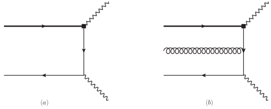
Figure 1: The subleading power two-particle and three-particle corrections to the vacuum-to-bottom-meson correlation function (2) at the tree-level accuracy, where the square box indicates an insertion of the weak vertex $\bar{q}\,\Gamma_{\mu}\,b$ and the waveline stands for the interpolating current $\bar{q}^{\prime}\,\not{n}\,\gamma_{5}\,q$ for the light pseudoscalar meson.

The first class of the subleading power contribution arises from retaining the higher-order terms in the heavy quark expansion of the hard-collinear quark propagator as depicted in Figure 1. Applying the computational strategy discussed in [97, 98], we proceed to write down the two-particle contribution to the QCD correlation function (2) at the tree-level accuracy

$$\Pi_{\mu,{\rm V},\rm NLP}^{\rm hc}(n\cdot p,\bar{n}\cdot p) = i\int d^{4}x\int\frac{d^{4}k}{(2\pi)^{4}}{\rm exp}\left(i\,k\cdot x\right)\,\frac{1}{(p-k)^{2}-m_{q}^{2}+i0}\,$$ (21)

$$\times\,\left\langle 0\left|\overline{q}^{\prime}(x)\,\not{n}\,\gamma_{5}\,(\not{p}-\not{k}+m_{q})\,\gamma_{\mu}\,h_{v}(0)\right|\bar{B}(p_{B})\right\rangle\,.$$

Implementing an expansion in powers of $\Lambda_{\rm QCD}/m_{b}$ for the hard-collinear quark propagator in (21) immediately leads to

$$\frac{(\not{p}-\not{k})+m_{q}}{(p-k)^{2}-m_{q}^{2}+i0} = \underbrace{\frac{1}{\bar{n}\cdot(p-k)}\,{\not{\bar{n}}\over 2}}+\underbrace{{1\over(p-k)^{2}}\,\left[\bar{n}\cdot p\,{\not{n}\over 2}-\not{k}+\frac{n\cdot k\,\,\bar{n}\cdot p}{\bar{n}\cdot(p-k)}\,{\not{\bar{n}}\over 2}\right]}$$ (22)

$$\hskip 28.45274pt{\rm LP}\hskip 119.50148pt{\rm NLP}$$

$$+\underbrace{{1\over(p-k)^{2}}\,\left[m_{q}+{m_{q}^{2}-m_{q^{\prime}}^{2}\over\bar{n}\cdot(p-k)}\,{\not{\bar{n}}\over 2}\right]}+\,...,$$

$$\hskip 42.67912pt{m_{q^{(\prime)}}\,\,\rm NLP}$$

where the abbreviation “LP” represents the leading-power effect discussed in Section 2. We can further cast the subleading-power terms displayed in the first line of (22) in the form

$$\Pi_{\mu,{\rm V},\rm NLP}^{\rm hc,\,I}(n\cdot p,\bar{n}\cdot p) = \int d^{4}x\int\frac{d^{4}k}{(2\pi)^{4}}\,{\rm exp}\left(i\,k\cdot x\right)\,\frac{1}{(p-k)^{2}+i0}\,$$ (23)

$$\times\,\bigg{\{}{\partial\over\partial x_{\rho}}\,\left\langle 0\left|\overline{q}^{\prime}(x)\,\not{n}\,\gamma_{5}\,\gamma_{\rho}\,\gamma_{\mu}\,h_{v}(0)\right|\bar{B}(p_{B})\right\rangle$$

$$\hskip 5.69046pt-{\bar{n}\cdot p\over\bar{n}\cdot(p-k)}\,(2\,v_{\rho}-\bar{n}_{\rho})\,{\partial\over\partial x_{\rho}}\,\left\langle 0\left|\overline{q}^{\prime}(x)\,\not{n}\,\gamma_{5}\,{\not{\bar{n}}\over 2}\,\gamma_{\mu}\,h_{v}(0)\right|\bar{B}(p_{B})\right\rangle\bigg{\}},\hskip 28.45274pt$$

by employing the standard technique of the integration by parts (IBP) as well as the precise relation between the four-vectors $n_{\alpha}=2\,v_{\alpha}-\bar{n}_{\alpha}$. Taking advantage of the well-known operator identities due to the HQET equations of motion

$$v_{\rho}\,{\partial\over\partial x_{\rho}}\,\left[\bar{q}^{\prime}(x)\,\Gamma\,h_{v}(0)\right] = i\,\int_{0}^{1}du\,\bar{u}\,\bar{q}^{\prime}(x)\,g_{s}\,G_{\alpha\beta}(ux)\,x^{\alpha}\,v^{\beta}\,\Gamma\,h_{v}(0)+(v\cdot\partial)\,\left[\bar{q}^{\prime}(x)\,\Gamma\,h_{v}(0)\right]\,,\hskip 22.76228pt$$ (24)

$${\partial\over\partial x_{\rho}}\bar{q}^{\prime}(x)\,\gamma_{\rho}\,\Gamma\,h_{v}(0) = -i\,\int_{0}^{1}du\,u\,\,\bar{q}^{\prime}(x)\,g_{s}\,G^{\lambda\rho}(ux)\,x_{\lambda}\,\gamma_{\rho}\,\Gamma\,h_{v}(0)+i\,m_{q^{\prime}}\,\bar{q}^{\prime}(x)\Gamma\,h_{v}(0)\,,$$ (25)

where the total translation operator $\partial_{\rho}$ acting on an arbitrary composite operator ${\cal O}(x_{1},...,x_{n})$ with $n$ space-time arguments is defined by

$$\partial_{\rho}\,{\cal O}(x_{1},...,x_{n})={\partial\over\partial y^{\rho}}\,{\cal O}(x_{1}+y,...,x_{n}+y)\bigg{|}_{y=0}\,,$$ (26)

we can then readily derive the factorized expressions for the effective NLP matrix elements of our interest at tree level

$$\Pi_{\rm NLP}^{\rm hc,\,I} = \left[{2\,{\cal F}_{B}(\mu)\,m_{B}\over n\cdot p}\right]\,\bigg{\{}\int_{0}^{\infty}d\omega_{1}\,\int_{0}^{\infty}d\omega_{2}\,\int_{0}^{1}du\,\frac{u\,\Phi_{4}(\omega_{1},\omega_{2},\mu)+\Psi_{4}(\omega_{1},\omega_{2},\mu)}{\left[\bar{n}\cdot p-\omega_{1}-u\,\omega_{2}\right]^{2}}\,$$ (27)

$$+\int_{0}^{\infty}d\omega\,\left(\bar{\Lambda}-{\omega+m_{q^{\prime}}\over 2}\right)\,\frac{\phi_{B}^{+}(\omega,\mu)}{\left[\bar{n}\cdot p-\omega\right]}\bigg{\}}+{\cal O}(\alpha_{s})\,,\hskip 28.45274pt$$

$$\tilde{\Pi}_{\rm NLP}^{\rm hc,\,I} = \left[-{2\,{\cal F}_{B}(\mu)\,m_{B}\over n\cdot p}\right]\,\bigg{\{}\int_{0}^{\infty}d\omega_{1}\,\int_{0}^{\infty}d\omega_{2}\,\int_{0}^{1}du\,\frac{\bar{u}\,(\bar{n}\cdot p+\omega_{1}+u\,\omega_{2})}{\left[\bar{n}\cdot p-\omega_{1}-u\,\omega_{2}\right]^{3}}\,\Psi_{5}(\omega_{1},\omega_{2},\mu)$$ (28)

$$+\int_{0}^{\infty}d\omega\,\left(\bar{\Lambda}-{\omega\over 2}\right)\,\frac{\omega\,\phi_{B}^{+}(\omega,\mu)}{\left[\bar{n}\cdot p-\omega\right]^{2}}\bigg{\}}+{\cal O}(\alpha_{s})\,.$$

The hadronic parameter $\bar{\Lambda}$ characterizing the “effective mass” of the bottom-meson state in HQET can be defined in an explicitly covariant and gauge invariant manner [99]

$$\bar{\Lambda}\equiv\frac{\langle 0|\bar{q}\,\,i\,v\cdot\overleftarrow{D}\,\Gamma\,h_{v}|\bar{B}_{q}(v)\rangle}{\langle 0|\bar{q}\,\Gamma\,h_{v}|\bar{B}_{q}(v)\rangle}\,.$$ (29)

Additionally, we have adopted the systematic parametrization of the three-body light-cone HQET matrix element at the twist-six accuracy [71]

$$\langle 0|\bar{q}_{\alpha}(\tau_{1}\,\bar{n})\,g_{s}\,G_{\mu\nu}(\tau_{2}\,\bar{n})\,h_{v\,\beta}(0)|\bar{B}_{v}\rangle$$

$$={{\cal F}_{B}(\mu)\,m_{B}\over 4}\,\bigg{[}(1+\not{v})\,\bigg{\{}(v_{\mu}\gamma_{\nu}-v_{\nu}\gamma_{\mu})\,\left[\hat{\Psi}_{A}(\tau_{1},\tau_{2},\mu)-\hat{\Psi}_{V}(\tau_{1},\tau_{2},\mu)\right]-i\,\sigma_{\mu\nu}\,\hat{\Psi}_{V}(\tau_{1},\tau_{2},\mu)$$

$$\hskip 11.38092pt-(\bar{n}_{\mu}\,v_{\nu}-\bar{n}_{\nu}\,v_{\mu})\,\hat{X}_{A}(\tau_{1},\tau_{2},\mu)+(\bar{n}_{\mu}\,\gamma_{\nu}-\bar{n}_{\nu}\,\gamma_{\mu})\,\left[\hat{W}(\tau_{1},\tau_{2},\mu)+\hat{Y}_{A}(\tau_{1},\tau_{2},\mu)\right]$$

$$\hskip 11.38092pt+\,i\,\epsilon_{\mu\nu\alpha\beta}\,\bar{n}^{\alpha}\,v^{\beta}\,\gamma_{5}\,\hat{\tilde{X}}_{A}(\tau_{1},\tau_{2},\mu)-\,i\,\epsilon_{\mu\nu\alpha\beta}\,\bar{n}^{\alpha}\,\gamma^{\beta}\,\gamma_{5}\,\hat{\tilde{Y}}_{A}(\tau_{1},\tau_{2},\mu)$$

$$\hskip 11.38092pt-\,(\bar{n}_{\mu}\,v_{\nu}-\bar{n}_{\nu}\,v_{\mu})\,\not{\bar{n}}\,\hat{W}(\tau_{1},\tau_{2},\mu)+\,(\bar{n}_{\mu}\,\gamma_{\nu}-\bar{n}_{\nu}\,\gamma_{\mu})\,\not{\bar{n}}\,\hat{Z}(\tau_{1},\tau_{2},\mu)\bigg{\}}\,\gamma_{5}\bigg{]}_{\beta\,\alpha}\,.$$ (30)

The momentum-space distribution amplitudes can be obtained by carrying out the Fourier transformation in the two light-cone variables $\tau_{1,2}$ [71, 100]

$$\Psi_{X}(\omega_{1},\omega_{2},\mu)=\int_{-\infty}^{+\infty}{d\tau_{1}\over 2\pi}\,\int_{-\infty}^{+\infty}{d\tau_{2}\over 2\pi}\,\,{\rm exp}\left[i(\omega_{1}\,\tau_{1}+\omega_{2}\,\tau_{2})\right]\,\hat{\Psi}_{X}(\tau_{1}-i0,\tau_{2}-i0,\mu)\,,$$

$$\Psi_{X}\in\left\{\Psi_{V},\,\Psi_{A},\,X_{A},\,Y_{A},\,\tilde{X}_{A},\,\tilde{Y}_{A},\,W,\,Z\right\},\,\,\hat{\Psi}_{X}\in\left\{\hat{\Psi}_{V},\,\hat{\Psi}_{A},\,\hat{X}_{A},\,\hat{Y}_{A},\,\hat{\tilde{X}}_{A},\,\hat{\tilde{Y}}_{A},\,\hat{W},\,\hat{Z}\right\}\,.\hskip 28.45274pt$$ (31)

To facilitate the construction of the perturbative factorization formulae, it turns out to be more advantageous to introduce the three-particle HQET distribution amplitudes with the definite collinear twist by virtue of the appearing invariant functions (see [101, 102] for further discussions on the comparison between dynamical twist and geometric twist )

$$\Phi_{3} = \Phi_{A}-\Phi_{V}\,,\qquad\hskip 108.12054pt\Phi_{4}=\Phi_{A}+\Phi_{V}\,,$$

$$\Psi_{4} = \Psi_{A}+X_{A}\,,\qquad\hskip 108.12054pt\tilde{\Psi}_{4}=\Psi_{V}-\tilde{X}_{A}\,,$$

$$\tilde{\Phi}_{5} = \Psi_{A}+\Psi_{V}+2\,Y_{A}-2\,\tilde{Y}_{A}+2\,W\,,\qquad\Psi_{5}=-\Psi_{A}+X_{A}-2\,Y_{A}\,,$$

$$\tilde{\Psi}_{5} = -\Psi_{V}-\tilde{X}_{A}+2\,\tilde{Y}_{A}\,,\qquad\hskip 62.59596pt\Phi_{6}=\Phi_{A}-\Phi_{V}+2\,Y_{A}+2\,W+2\,\tilde{Y}_{A}-4\,Z\,.\hskip 28.45274pt$$ (32)

Applying the standard factorization method, we can compute the power-suppressed contributions presented in the second line of (22) due to the non-vanishing quark masses

$$\Pi_{\rm NLP}^{\rm hc,\,II} = \left[-{{\cal F}_{B}(\mu)\,m_{B}\over n\cdot p}\right]\,\int_{0}^{\infty}d\omega\,\frac{m_{q}}{\bar{n}\cdot p-\omega}\,\phi_{B}^{-}(\omega,\mu)+{\cal O}(\alpha_{s})\,,$$ (33)

$$\tilde{\Pi}_{\rm NLP}^{\rm hc,\,II} = \left[-{{\cal F}_{B}(\mu)\,m_{B}\over n\cdot p}\right]\,\int_{0}^{\infty}d\omega\,\frac{\left(m_{q}^{2}-m_{q^{\prime}}^{2}\right)}{\left[\bar{n}\cdot p-\omega\right]^{2}}\,\,\phi_{B}^{-}(\omega,\mu)+{\cal O}(\alpha_{s})\,.$$ (34)

In contrast to the NLP active-quark mass corrections, the newly identified spectator-quark mass contributions cannot generate the large-recoil symmetry breaking effects at ${\cal O}(\alpha_{s}^{0})$.

Along the same vein, we can derive the soft-collinear factorization formulae for the particular subleading-power corrections to the correlation function $\Pi_{\mu,{\rm T}}$ from the higher-order terms in the heavy quark expansion of the hard-collinear quark propagator

$$\Pi_{\rm T,\,NLP}^{\rm hc,\,I}=\left(\tilde{\Pi}_{\rm NLP}^{\rm hc,\,I}-\Pi_{\rm NLP}^{\rm hc,\,I}\right)+{\cal O}(\alpha_{s})\,,\qquad\Pi_{\rm T,\,NLP}^{\rm hc,\,II}=\left(\tilde{\Pi}_{\rm NLP}^{\rm hc,\,II}-\Pi_{\rm NLP}^{\rm hc,\,II}\right)+{\cal O}(\alpha_{s})\,.$$ (35)

These interesting constraints can be attributed to the classical HQET equation of motion

$$\left(\sigma_{\mu\nu}\,q^{\nu}\right)\,\mathds{1}\,h_{v}=\left(\sigma_{\mu\nu}\,q^{\nu}\right)\,\not{v}\,h_{v}=\left(-{i\over 2}\right)\,\left[\bar{n}\cdot q\,n_{\mu}-n\cdot q\,\bar{n}_{\mu}\right]\,\left({\not{n}\over 2}-{\not{\bar{n}}\over 2}\right)\,h_{v}\,.$$ (36)

Including the non-Eikonal gluonic interaction with the bottom-quark field in the higher-order corrections to the vacuum-to-bottom-meson correlation functions will generally invalidate such symmetry relations.

Expressing the established NLP factorization formulae in the dispersion forms and equating the achieved spectral representations for the correlation functions with the corresponding hadronic dispersion relations (16) allows us to construct the desired LCSR for the power-suppressed contributions from the expanded hard-collinear quark propagator

$$f_{M}\,\,{\rm exp}\left[-{m_{M}^{2}\over n\cdot p\,\,\omega_{M}}\right]\,\,\left\{\frac{n\cdot p}{m_{B}}\,f_{BM,\,\rm NLP}^{+,\,\rm hc}(q^{2})\,,\,\,\,f_{BM,\,\rm NLP}^{0,\,\rm hc}(q^{2})\,,\,\,\,\frac{n\cdot p}{m_{B}+m_{M}}\,f_{BM,\,\rm NLP}^{T,\,\rm hc}(q^{2})\right\}\,$$

$$={\mathcal{F}_{B}(\mu)\over n\cdot p}\,\bigg{[}\int_{0}^{\omega_{s}}\,d\omega_{1}\,\,\int_{0}^{\infty}\,{d\omega_{2}\over\omega_{2}}\,\,\bigg{\{}e^{-{\omega_{1}+\omega_{2}\over\omega_{M}}}\,\varrho_{\rm NLP}^{\rm hc,\,I}(\omega_{1},\omega_{2},\mu)\,\theta(\omega_{s}-\omega_{1}-\omega_{2})$$

$$\hskip 14.22636pt+\,\left[\left(e^{-{\omega_{1}\over\omega_{M}}}-e^{-{\omega_{s}\over\omega_{M}}}\right)\,\theta(\omega_{1}+\omega_{2}-\omega_{s})+\left(e^{-{\omega_{1}\over\omega_{M}}}-e^{-{\omega_{1}+\omega_{2}\over\omega_{M}}}\right)\,\theta(\omega_{s}-\omega_{1}-\omega_{2})\right]$$

$$\hskip 14.22636pt\times\,\varrho_{\rm NLP}^{\rm hc,\,II}(\omega_{1},\omega_{2},\mu)+e^{-{\omega_{1}\over\omega_{M}}}\,\varrho_{\rm NLP}^{\rm hc,\,III}(\omega_{1},\omega_{2},\mu)\bigg{\}}+\int_{0}^{\omega_{s}}\,d\omega\,\,e^{-{\omega\over\omega_{M}}}\,\,\tilde{\varrho}_{\rm NLP}^{\rm hc}(\omega,\mu)\bigg{]}+{\cal O}(\alpha_{s})\,.\hskip 28.45274pt$$ (37)

The yielding expressions for the emerged coefficient functions $\varrho_{\rm NLP}^{\rm hc,\,(I,II,III)}$ and $\tilde{\varrho}_{\rm NLP}^{\rm hc}$ can be explicitly written as

$$\varrho_{\rm NLP}^{\rm hc,\,I} = 2\,\left\{{\omega_{1}+\omega_{2}\over\omega_{2}}\,\Psi_{5}(\omega_{1},\omega_{2},\mu)\,-\,\kappa_{i}\,\left(\Phi_{4}+\Psi_{4})(\omega_{1},\omega_{2},\mu\right)\right\}\,,$$ (38)

$$\varrho_{\rm NLP}^{\rm hc,\,II} = -2\,\left({\omega_{M}\over\omega_{2}}\right)\,\left[\Psi_{5}(\omega_{1},\omega_{2},\mu)+\kappa_{i}\,\Phi_{4}(\omega_{1},\omega_{2},\mu)\right]\,,$$ (39)

$$\varrho_{\rm NLP}^{\rm hc,\,III} = 2\,\left\{\left({d\over d\omega_{1}}-{1\over\omega_{2}}\right)\,\left[\omega_{1}\,\Psi_{5}(\omega_{1},\omega_{2},\mu)\right]\,-\,\kappa_{i}\,\Phi_{4}(\omega_{1},\omega_{2},\mu)\right\}\,,$$ (40)

$$\tilde{\varrho}_{\rm NLP}^{\rm hc} = \left[1-\left({\omega_{s}-\omega\over\omega}\right)\,{m_{q}^{2}-m_{q^{\prime}}^{2}\over\omega_{s}\,\omega_{M}}\,+\left(\omega-2\,\bar{\Lambda}-{m_{q}^{2}-m_{q^{\prime}}^{2}\over\omega_{s}}\right)\,{d\over d\omega}\right]\,\left[\omega\,\phi_{B}^{-}(\omega,\mu)\right]$$ (41)

$$+\,\kappa_{i}\,\left[\left(\omega-2\,\bar{\Lambda}\right)\,\phi_{B}^{+}(\omega,\mu)+\left(m_{q}+m_{q^{\prime}}\right)\,\phi_{B}^{-}(\omega,\mu)\right]\,,$$

where the non-universal $\kappa_{i}$-factors are responsible for the symmetry-breaking effects

$$\kappa_{+}=-\kappa_{0}={(n\cdot p-m_{B})/m_{B}}\,,\qquad\kappa_{T}=-1\,.$$ (42)

Importantly, we have further verified that the newly derived sum rules (37) for the light-quark-mass insensitive NLP corrections from the heavy quark expansion of the hard-collinear propagator are consistent with the previous computations for the semileptonic $B\to D\ell\bar{\nu}_{\ell}$ form factors accomplished in [40].

3.2 The NLP contribution from the subleading effective current

We now proceed to determine the second class of the subleading-power correction to the exclusive $B_{d,s}\to\pi,K$ form factors arising from the peculiar higher-order term in the ${\rm SCET}_{\rm I}$ representation of the heavy-to-light transition current $\bar{q}\,\Gamma_{\mu}\,b$ [103]

$$J^{\rm(A2)}\supset(\bar{\xi}_{\rm hc}\,W_{\rm hc})\,\,\Gamma\,\,\left({i\,\overrightarrow{\not{D}}_{\top}\over 2\,m_{b}}\right)\,\,h_{v}+...\,,\qquad D_{\top}^{\mu} \equiv D^{\mu}-(v\cdot D)\,v^{\mu}\,,$$ (43)

which corresponds to the standard ${\rm QCD}\to{\rm HQET}$ matching for the bottom-quark field

$$b(x)={\rm exp}\left(-i\,m_{b}\,v\cdot x\right)\,\bigg{[}1+{i\,\overrightarrow{{\not{D}}}_{\top}\over 2\,m_{b}}+{(v\cdot\overrightarrow{D})\,\overrightarrow{{\not{D}}}_{\top}\over 4\,m_{b}^{2}}-{\overrightarrow{{\not{D}}}_{\top}\,\overrightarrow{{\not{D}}}_{\top}\over 8\,m_{b}^{2}}+{\cal O}\left({1\over m_{b}^{3}}\right)\bigg{]}\,h_{v}(x)\,.$$ (44)

It is then straightforward to express the resulting NLP contribution to the vacuum-to-$B$-meson correlation function (2) in the following form

$$\Pi_{\mu,{\rm V},\rm NLP}^{\rm(A2)}(n\cdot p,\bar{n}\cdot p) = -\left({n\cdot p\over 4\,m_{b}}\right)\,\int d^{4}x\int\frac{d^{4}k}{(2\pi)^{4}}{\rm exp}\left(i\,k\cdot x\right)\,\frac{1}{(p-k)^{2}-m_{q}^{2}+i0}\,$$ (45)

$$\times\,\left\langle 0\left|\overline{q}^{\prime}(x)\,\not{n}\,\gamma_{5}\,\not{\bar{n}}\,\gamma_{\mu}\,\overrightarrow{{\not{D}}}_{\top}\,h_{v}(0)\right|\bar{B}(p_{B})\right\rangle$$

$$= -\left({n\cdot p\over 2\,m_{b}}\right)\,\int d^{4}x\int\frac{d^{4}k}{(2\pi)^{4}}{\rm exp}\left(i\,k\cdot x\right)\,\frac{\bar{n}_{\mu}}{(p-k)^{2}-m_{q}^{2}+i0}\,$$

$$\times\,\left\langle 0\left|\overline{q}^{\prime}(x)\,\left(\overrightarrow{{\not{D}}}_{\top}\,\,\not{n}\,+\,2\,\bar{n}\cdot\overrightarrow{D}_{\top}\right)\,\gamma_{5}\,h_{v}(0)\right|\bar{B}(p_{B})\right\rangle\,,$$

where we have employed the lowest-order equation of motion of the effective heavy-quark field

$$i\,v\cdot\overrightarrow{D}\,h_{v}=0\,.$$ (46)

This evidently permits the replacement $i\,\overrightarrow{\not{D}}_{\top}\,h_{v}\to i\,\overrightarrow{\not{D}}\,h_{v}$ in the effective weak current at the NLP accuracy. Taking advantage of an additional HQET operator identity [69, 70, 71]

$$\bar{q}^{\prime}(x)\,\Gamma\,{\overrightarrow{D}}_{\rho}\,h_{v}(0) = \partial_{\rho}\left[\bar{q}^{\prime}(x)\,\Gamma\,h_{v}(0)\right]\,+\,i\,\int_{0}^{1}du\,\bar{u}\,\,\bar{q}^{\prime}(x)\,g_{s}\,G_{\lambda\rho}(ux)\,x^{\lambda}\,\Gamma\,h_{v}(0)$$ (47)

$$-\,{\partial\over\partial x^{\rho}}\bar{q}^{\prime}(x)\,\Gamma\,h_{v}(0)\,,$$

in combination with the two operator relations displayed in (24) and (25), we can construct the perturbative factorization formula for the non-local hadronic matrix element in (45)

$$\Pi_{\rm NLP}^{\rm(A2)} = {\cal O}(\alpha_{s})\,,$$ (48)

$$\tilde{\Pi}_{\rm NLP}^{\rm(A2)} = \left[{\mathcal{F}_{B}(\mu)\,m_{B}\over 2\,m_{b}}\right]\,\bigg{\{}\int_{0}^{\infty}\,d\omega_{1}\,\int_{0}^{\infty}\,d\omega_{2}\,{2\,(\Psi_{4}+\Phi_{4})(\omega_{1},\omega_{2},\mu)\over(\omega_{1}-\bar{n}\cdot p)\,(\omega_{1}+\omega_{2}-\bar{n}\cdot p)}\,$$ (49)

$$+\,\int_{0}^{\infty}\,{d\omega\over\omega-\bar{n}\cdot p}\,\left[\left(\omega-2\,\bar{\Lambda}\right)\,\phi_{B}^{+}(\omega,\mu)+\left(\omega-\bar{\Lambda}+m_{q^{\prime}}\right)\,\phi_{B}^{-}(\omega,\mu)\right]\bigg{\}}+{\cal O}(\alpha_{s})\,.$$

Applying the analogous computational strategy, we can further compute the yielding NLP correction to the correlation function $\Pi_{\mu,{\rm T}}$ at tree level

$$\Pi_{\rm T,\,NLP}^{\rm(A2)}=-\left(\tilde{\Pi}_{\rm NLP}^{\rm(A2)}-\Pi_{\rm NLP}^{\rm(A2)}\right)+{\cal O}(\alpha_{s})\,.$$ (50)

We remark in passing that such an interesting constraint (50) differs from the previously established relations (35) for the NLP corrections from the HQET expansion of the hard-collinear quark propagator by an overall factor of “$-1$”. This observation can be traced back to the anti-commutation relation $\left\{\not{v},\overrightarrow{\not{D}}_{\top}\right\}\,h_{v}=0$, thus ensuring an exact algebraic identity

$$\left(\sigma_{\mu\nu}\,q^{\nu}\right)\,\left({i\,\overrightarrow{\not{D}}_{\top}\over 2\,m_{b}}\right)\,h_{v} = \left({i\over 2}\right)\,\left[\bar{n}\cdot q\,n_{\mu}-n\cdot q\,\bar{n}_{\mu}\right]\,\left({\not{n}\over 2}-{\not{\bar{n}}\over 2}\right)\,\left({i\,\overrightarrow{\not{D}}_{\top}\over 2\,m_{b}}\right)\,h_{v}\,.$$ (51)

Matching the spectral representations for the established soft-collinear factorization formulae (49) and (50) with the corresponding hadronic dispersion relations (16) enables us to derive the final expressions for the NLP sum rules of the $B_{d,s}\to\pi,K$ decay form factors

$$f_{M}\,\,{\rm exp}\left[-{m_{M}^{2}\over n\cdot p\,\,\omega_{M}}\right]\,\,\left\{\frac{n\cdot p}{m_{B}}\,f_{BM,\,\rm NLP}^{+,\,\rm(A2)}(q^{2})\,,\,\,\,f_{BM,\,\rm NLP}^{0,\,\rm(A2)}(q^{2})\,,\,\,\,{\color[rgb]{0.00,0.00,1.00}\left[-\frac{n\cdot p}{m_{B}+m_{M}}\right]}\,f_{BM,\,\rm NLP}^{T,\,\rm(A2)}(q^{2})\right\}\,$$

$$={\mathcal{F}_{B}(\mu)\over n\cdot p}\,\bigg{[}\int_{0}^{\omega_{s}}\,d\omega_{1}\,\,\int_{0}^{\infty}\,{d\omega_{2}\over\omega_{2}}\,\,\bigg{\{}e^{-{\omega_{1}+\omega_{2}\over\omega_{M}}}\,\varrho_{\rm NLP}^{\rm(A2),\,I}(\omega_{1},\omega_{2},\mu)\,\theta(\omega_{s}-\omega_{1}-\omega_{2})$$

$$\hskip 51.21504pt+\,e^{-{\omega_{1}\over\omega_{M}}}\,\varrho_{\rm NLP}^{\rm(A2),\,II}(\omega_{1},\omega_{2},\mu)\bigg{\}}\,\,+\int_{0}^{\omega_{s}}\,d\omega\,\,e^{-{\omega\over\omega_{M}}}\,\,\tilde{\varrho}_{\rm NLP}^{\rm(A2)}(\omega,\mu)\bigg{]}+{\cal O}(\alpha_{s})\,.$$ (52)

The non-perturbative coefficient functions $\varrho_{\rm NLP}^{\rm(A2),\,(I,II)}$ and $\tilde{\varrho}_{\rm NLP}^{\rm(A2)}$ can be expressed in terms of the two-particle and three-particle HQET distribution amplitudes

$$\varrho_{\rm NLP}^{\rm(A2),\,I}=-{n\cdot p\over m_{b}}\,\left[\left(\Phi_{4}+\Psi_{4})(\omega_{1},\omega_{2},\mu\right)\right]\,,\qquad\varrho_{\rm NLP}^{\rm(A2),\,II}={n\cdot p\over m_{b}}\,\left(\Phi_{4}+\Psi_{4})(\omega_{1},\omega_{2},\mu\right)\,,$$ (53)

$$\tilde{\varrho}_{\rm NLP}^{\rm(A2)}={n\cdot p\over 2\,m_{b}}\,\left[\left(\omega-2\,\bar{\Lambda}\right)\,\phi_{B}^{+}(\omega,\mu)+\left(\omega-\bar{\Lambda}+m_{q^{\prime}}\right)\,\phi_{B}^{-}(\omega,\mu)\right]\,.\hskip 28.45274pt$$ (54)

Remarkably, the considered NLP corrections to the heavy-to-light form factors from the effective matrix elements of the subleading ${\rm SCET}_{\rm I}$ current $J^{\rm(A2)}$ preserve the well-known symmetry relation between the vector and scalar form factors, but violate the large-recoil symmetry of the vector and tensor form factors already at ${\cal O}(\alpha_{s}^{0})$.

3.3 The NLP contribution form the higher-twist two-particle and three-particle LCDAs

As emphasized repeatedly in [104, 105], the systematic and consistent description of the higher-twist corrections to exclusive hard reactions in QCD will require us to simultaneously take into account the transverse-momentum dependence of the valence (anti)-quarks in the leading Fock-state wavefunction and the subleading distribution amplitudes of the non-minimal partonic configuration with additional gluons and/or quark-antiquark pairs. Including the off-light-cone corrections to the renormalized two-body non-local HQET matrix element at the ${\cal O}(x^{2})$ accuracy discussed in [71]

$$\langle 0|\left(\bar{q}^{\prime}\,Y_{s}\right)_{\beta}(x)\,\left(Y_{s}^{{\dagger}}\,h_{v}\right)_{\alpha}(0)|\bar{B}(v)\rangle$$

$$=-\frac{i\,{\cal F}_{B}(\mu)\,m_{B}}{4}\,\int_{0}^{\infty}\,d\omega\,\,{\rm exp}\left[{-i\,\omega\,v\cdot x}\right]\,\bigg{\{}\frac{1+\not{v}}{2}\,\,\bigg{[}2\,\left(\phi_{B}^{+}(\omega,\mu)+{\color[rgb]{0.00,0.00,1.00}x^{2}\,g_{B}^{+}(\omega,\mu)}\right)$$

$$\hskip 14.22636pt-{1\over v\cdot x}\,\left[\left(\phi_{B}^{+}(\omega,\mu)-\phi_{B}^{-}(\omega,\mu)\right)+{\color[rgb]{0.00,0.00,1.00}x^{2}\,\left(g_{B}^{+}(\omega,\mu)-g_{B}^{-}(\omega,\mu)\right)}\right]\,\not{x}\bigg{]}\,\gamma_{5}\bigg{\}}_{\alpha\beta}\,,$$ (55)

we can proceed to construct the tree-level factorization formulae for the two-particle higher-twist corrections to the three invariant functions $\Pi$, $\tilde{\Pi}$ and $\Pi_{\rm T}$ [35]

$$\Pi_{\rm NLP}^{\rm 2PHT} = {\cal O}(\alpha_{s})\,,$$ (56)

$$\tilde{\Pi}_{\rm NLP}^{\rm 2PHT} = \left[{2\,\mathcal{F}_{B}(\mu)\,m_{B}\over n\cdot p}\right]\,\bigg{\{}\int_{0}^{\infty}\,d\omega_{1}\,\int_{0}^{\infty}\,d\omega_{2}\,\int_{0}^{1}\,du\,\,{\bar{u}\,\Psi_{5}(\omega_{1},\omega_{2},\mu)\over\left[\bar{n}\cdot p-\omega_{1}-u\,\omega_{2}\right]^{2}}\,$$ (57)

$$-\,2\,\int_{0}^{\infty}\,d\omega\,\,{\hat{g}_{B}^{-}(\omega,\mu)\over\left[\bar{n}\cdot p-\omega\right]^{2}}\,\bigg{\}}+{\cal O}(\alpha_{s})\,,$$

$$\Pi_{\rm T,\,NLP}^{\rm 2PHT} = \left(\tilde{\Pi}_{\rm NLP}^{\rm 2PHT}-\Pi_{\rm NLP}^{\rm 2PHT}\right)+{\cal O}(\alpha_{s})\,.$$ (58)

In the above derivation we have employed the nontrivial constraint on the momentum-space distribution amplitudes due to the HQET equations of motion

$$-2\,{d^{2}g_{B}^{-}(\omega,\mu)\over d\omega^{2}} = \left[{3\over 2}+(\omega-\bar{\Lambda})\,{d\over d\omega}\right]\,\phi_{B}^{-}(\omega,\mu)-\left({1\over 2}\right)\,\phi_{B}^{+}(\omega,\mu)$$ (59)

$$+\int_{0}^{\infty}\,{d\omega_{2}\over\omega_{2}}\,\left({d\over d\omega}-{1\over\omega_{2}}\right)\,\Psi_{5}(\omega,\omega_{2},\mu)+\int_{0}^{\omega}\,{d\omega_{2}\over\omega_{2}^{2}}\,\Psi_{5}(\omega-\omega_{2},\omega_{2},\mu)\,.\hskip 28.45274pt$$

This allows us to decompose the higher-twist LCDA $g_{B}^{-}(\omega,\mu)$ into the “genuine” twist-five three-particle distribution amplitude $\Psi_{5}(\omega_{1},\omega_{2},\mu)$ and the lower-twist “Wandzura-Wilczek” contribution labelled as $\hat{g}_{B}^{-}(\omega,\mu)$, which can be explicitly expressed in terms of the customary two-particle $B$-meson distribution amplitudes

$$\hat{g}_{B}^{-}(\omega,\mu)=\left({1\over 4}\right)\,\int_{\omega}^{\infty}\,d\rho\,\left\{(\rho-\omega)\,\left[\phi_{B}^{+}(\rho)-\phi_{B}^{-}(\rho)\right]-2\,(\bar{\Lambda}-\rho)\,\phi_{B}^{-}(\rho)\right\}\,.$$ (60)

Applying further the light-cone expansion for the massive-quark propagator in the background gluon field up to the gluon field strength terms without the covariant derivatives [106, 20] (see also [107, 108] for an alternative representation)

$$S(x,0,m_{q}) \equiv \langle 0|{\rm T}\,\{q(x),\,\bar{q}(0)\}|0\rangle$$ (61)

$$\supset i\,g_{s}\,\int_{-\infty}^{+\infty}\,\,{d^{4}\ell\over(2\pi)^{4}}\,{\rm exp}\left[{-i\,\ell\cdot x}\right]\,\int_{0}^{1}\,du\,\left[{u\,x_{\mu}\,\gamma_{\nu}\over\ell^{2}-m_{q}^{2}}-\frac{(\not{\ell}+m_{q})\,\sigma_{\mu\nu}}{2\,(\ell^{2}-m_{q}^{2})^{2}}\right]\,G^{\mu\nu}(u\,x)\,,\hskip 28.45274pt$$

we can continue to write down the tree-level factorized expressions for the yielding three-particle higher-twist corrections to the vacuum-to-$B$-meson correlation functions (2) displayed in Figure 1(b) [35]

$$\Pi_{\rm NLP}^{\rm 3PHT} = \left[{{\cal F}_{B}(\mu)\,m_{B}\over n\cdot p}\right]\,\int_{0}^{\infty}d\omega_{1}\,\int_{0}^{\infty}d\omega_{2}\,\int_{0}^{1}du\,\frac{1}{\left[\bar{n}\cdot p-\omega_{1}-u\,\omega_{2}\right]^{2}}\,$$ (62)

$$\times\,\left\{2\,\bar{u}\,\Phi_{4}(\omega_{1},\omega_{2},\mu)+{m_{q}\over n\cdot p}\left(\Psi_{5}-\tilde{\Psi}_{5}\right)(\omega_{1},\omega_{2},\mu)\right\}+{\cal O}(\alpha_{s})\,,$$

$$\tilde{\Pi}_{\rm NLP}^{\rm 3PHT} = \left[{{\cal F}_{B}(\mu)\,m_{B}\over n\cdot p}\right]\,\int_{0}^{\infty}d\omega_{1}\,\int_{0}^{\infty}d\omega_{2}\,\int_{0}^{1}du\,\frac{1}{\left[\bar{n}\cdot p-\omega_{1}-u\,\omega_{2}\right]^{2}}\,$$ (63)

$$\times\,\left\{\left[(2\,u-1)\,\Psi_{5}-\tilde{\Psi}_{5}\right](\omega_{1},\omega_{2},\mu)-{2\,m_{q}\over n\cdot p}\,\Phi_{6}(\omega_{1},\omega_{2},\mu)\right\}+{\cal O}(\alpha_{s})\,,\hskip 28.45274pt$$

$$\Pi_{\rm T,\,NLP}^{\rm 3PHT} = \left(\tilde{\Pi}_{\rm NLP}^{\rm 3PHT}-\Pi_{\rm NLP}^{\rm 3PHT}\right)+{\cal O}(\alpha_{s})\,.$$ (64)

Adding together the obtained two-particle and three-particle subleading twist corrections in the dispersion form and implementing the standard continuum subtraction procedure with the parton-hadron duality ansätz leads to the following sum rules for the NLP contributions to the semileptonic $B_{d,s}\to\pi,K$ form factors

$$f_{M}\,\,{\rm exp}\left[-{m_{M}^{2}\over n\cdot p\,\,\omega_{M}}\right]\,\,\left\{\frac{n\cdot p}{m_{B}}\,f_{BM,\,\rm NLP}^{+,\,\rm HT}(q^{2})\,,\,\,\,f_{BM,\,\rm NLP}^{0,\,\rm HT}(q^{2})\,,\,\,\,\frac{n\cdot p}{m_{B}+m_{M}}\,f_{BM,\,\rm NLP}^{T,\,\rm HT}(q^{2})\right\}\,$$

$$={\mathcal{F}_{B}(\mu)\over n\cdot p}\,\bigg{[}\int_{0}^{\omega_{s}}\,d\omega_{1}\,\,\int_{0}^{\infty}\,{d\omega_{2}\over\omega_{2}}\,\,\bigg{\{}e^{-{\omega_{1}+\omega_{2}\over\omega_{M}}}\,\varrho_{\rm NLP}^{\rm HT,\,I}(\omega_{1},\omega_{2},\mu)\,\theta(\omega_{s}-\omega_{1}-\omega_{2})$$

$$\hskip 14.22636pt+\,\left[\left(e^{-{\omega_{1}\over\omega_{M}}}-e^{-{\omega_{s}\over\omega_{M}}}\right)\,\theta(\omega_{1}+\omega_{2}-\omega_{s})+\left(e^{-{\omega_{1}\over\omega_{M}}}-e^{-{\omega_{1}+\omega_{2}\over\omega_{M}}}\right)\,\theta(\omega_{s}-\omega_{1}-\omega_{2})\right]$$

$$\hskip 14.22636pt\times\,\varrho_{\rm NLP}^{\rm HT,\,II}(\omega_{1},\omega_{2},\mu)+e^{-{\omega_{1}\over\omega_{M}}}\,\varrho_{\rm NLP}^{\rm HT,\,III}(\omega_{1},\omega_{2},\mu)\bigg{\}}\,\,+\int_{0}^{\omega_{s}}\,d\omega\,\,e^{-{\omega\over\omega_{M}}}\,\,\tilde{\varrho}_{\rm NLP}^{\rm HT}(\omega,\mu)\bigg{]}+{\cal O}(\alpha_{s})\,.\hskip 28.45274pt$$ (65)

The explicit expressions for the coefficient functions $\varrho_{\rm NLP}^{\rm HT,\,(I,II,III)}$ and $\tilde{\varrho}_{\rm NLP}^{\rm HT}$ are given by

$$\varrho_{\rm NLP}^{\rm HT,\,I} = \left[-\left(1+{m_{q}\over n\cdot p}\,\kappa_{i}\right)\,\left(\Psi_{5}-\tilde{\Psi}_{5}\right)(\omega_{1},\omega_{2},\mu)\right]+{2\,m_{q}\over n\cdot p}\,\Phi_{6}(\omega_{1},\omega_{2},\mu),$$ (66)

$$\varrho_{\rm NLP}^{\rm HT,\,III} = \left[2\,\kappa_{i}\,\Phi_{4}(\omega_{1},\omega_{2},\mu)+\left(1+{m_{q}\over n\cdot p}\,\kappa_{i}\right)\,\left(\Psi_{5}-\tilde{\Psi}_{5}\right)(\omega_{1},\omega_{2},\mu)\right]-{2\,m_{q}\over n\cdot p}\,\Phi_{6}(\omega_{1},\omega_{2},\mu),\hskip 19.91684pt$$ (67)

$$\varrho_{\rm NLP}^{\rm HT,\,II} = -2\,\left({\omega_{M}\over\omega_{2}}\right)\,\kappa_{i}\,\Phi_{4}(\omega_{1},\omega_{2},\mu)\,,\qquad\hskip 56.9055pt\tilde{\varrho}_{\rm NLP}^{\rm HT}=-4\,{d\hat{g}_{B}^{-}(\omega,\mu)\over d\omega}.$$ (68)

Interestingly, the obtained tree-level sum rules for the two-particle higher-twist contributions are independent of the non-universal $\kappa_{i}$-factors, thus maintaining the large-recoil symmetry relations of the considered bottom-meson decay form factors. According to our power-counting scheme for the intrinsic LCSR parameters $\omega_{s}\sim\omega_{M}\sim{\cal O}(\Lambda_{\rm QCD}^{2}/m_{b})$, we can immediately determine the desired scaling behaviours of the two-particle and three-particle higher-twist corrections at ${\cal O}(\alpha_{s}^{0})$ in the heavy quark limit [35]

$$f_{BM,\,\rm NLP}^{+,\,\rm HT}\sim f_{BM,\,\rm NLP}^{0,\,\rm HT}\sim f_{BM,\,\rm NLP}^{T,\,\rm HT}\sim{\cal O}((\Lambda_{\rm QCD}/m_{b})^{5/2})\,,$$ (69)

which turn out to be suppressed by one power of $\Lambda_{\rm QCD}/m_{b}$ in comparison with the leading-power SCET sum rules (18) and (19). It is however important to emphasize that evaluating the (currently unknown) higher-order radiative corrections to the three-particle twist-three $B$-meson LCDA contributions can actually bring about the unsuppressed symmetry-preserving effects for the exclusive $B_{d,s}\to\pi,K$ form factors in the heavy quark expansion. This observation can be understood from the very fact that the two-particle twist-three distribution amplitude $\phi_{B}^{-}(\omega,\mu)$ appearing in the tree-level sum rules can be generated by the one-loop renormalization of the three-particle $B$-meson LCDA $\Phi_{3}(\omega_{1},\omega_{2},\mu)$ [109, 88] (see [110] for further discussions in the SCET framework).

3.4 The NLP contribution form the higher-twist four-particle effects

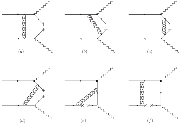
Figure 2: Diagrammatic representations of the twist-five and twist-six four-particle corrections to the considered vacuum-to-bottom-meson correlation functions (2) at the ${\cal O}(\alpha_{s})$ accuracy.

We are now in a position to compute the NLP corrections to the heavy-to-light bottom-meson decay form factors from the twist-five and twist-six four-particle LCDA contributions in the factorization approximation, following the computational prescriptions for the electromagnetic pion form factor at intermediate momentum transfer [111], the exclusive photon-pion transition form factor $\gamma^{\ast}\gamma\to\pi$ [72] and the radiative leptonic $B\to\gamma\ell\bar{\nu}_{\ell}$ decay amplitude [73]. Evaluating the lowest-order Feynman diagrams in Figure 2 straightforwardly leads to the factorized expressions for such non-leading Fock-state corrections

$$\Pi_{\rm NLP}^{\rm 4P} = {\cal O}(\alpha_{s}^{2})$$ (70)

$$\tilde{\Pi}_{\rm NLP}^{\rm 4P} = {2\,\pi\over 3}\,\frac{\alpha_{s}(\mu)\,C_{F}\,\langle\bar{q}^{\prime}q^{\prime}\rangle}{n\cdot p\,\bar{n}\cdot p}\,{\cal F}_{B}(\mu)\,m_{B}\,\int_{0}^{\infty}\frac{d\omega}{\omega-\bar{n}\cdot p}\,{\phi_{B}^{+}(\omega,\mu)\over\omega}\,$$ (71)

$$\times\,\left\{{2\,\bar{n}\cdot p\over\omega}\,\left[1+{\bar{n}\cdot p-\omega\over\omega}\,\ln{\bar{n}\cdot p-\omega\over\bar{n}\cdot p}\right]-1+{\langle\bar{q}q\rangle\over\langle\bar{q}^{\prime}q^{\prime}\rangle}\,{\omega\over\omega-\bar{n}\cdot p}\right\}\,+{\cal O}(\alpha_{s}^{2})\,,\hskip 22.76228pt$$

$$\Pi_{\rm T,\,NLP}^{\rm 4P} = \left(\tilde{\Pi}_{\rm NLP}^{\rm 4P}-\Pi_{\rm NLP}^{\rm 4P}\right)+{\cal O}(\alpha_{s}^{2})\,.$$ (72)

It is perhaps worth mentioning that the determined four-particle contributions to the vacuum-to-bottom-meson correlation functions (2) from the particular diagram (e) in Figure 2 can be most conveniently computed with the familiar background-field expansion of the quark propagator on the light-cone [106]

$$\langle 0|{\rm T}\,\{q(x),\,\bar{q}(0)\}|0\rangle \supset \frac{\Gamma({d/2}-1)}{8\,\pi^{d/2}\,(-x^{2})^{d/2-1}}\,\int_{0}^{1}du\,u\,\bar{u}\,\not{x}\,x_{\nu}\,D^{\mu}\,g_{s}\,G^{\mu\nu}(ux)$$ (73)

$$+\,\frac{\Gamma({d/2}-2)}{16\,\pi^{d/2}\,(-x^{2})^{d/2-2}}\,\int_{0}^{1}du\,\left(u\,\bar{u}-{1\over 2}\right)\,D^{\mu}\,g_{s}\,G^{\mu\nu}(ux)\,\gamma^{\nu}\,,$$

together with the classical equation of motion in QCD

$$D^{\mu}\,G_{\mu\nu}^{a}=-i\,g_{s}\,\sum_{q}\,\bar{q}\,\gamma_{\nu}\,T^{a}\,q.$$ (74)

Additionally, our explicit calculations of the three diagrams (a), (b) and (c) in Figure 2 indicate that they can only generate the yet higher-power corrections in the heavy quark expansion when compared with the dominating contributions from the diagrams (d) and (e). These enlightening pattern differs drastically from the counterpart NLP contributions to the two helicity form factors of $B\to\gamma\ell\bar{\nu}_{\ell}$, due to the longitudinally polarized pseudoscalar-meson current in the former and the transversely polarized on-shell photon state in the latter. Moreover, the remaining diagram (f) in Figure 2 turns out to be insensitive to both the hard and hard-collinear QCD dynamics.

We can proceed to work out the dispersion representations for the four-particle corrections to the invariant functions $\Pi$, $\tilde{\Pi}$ and $\Pi_{\rm T}$ at ${\cal O}(\alpha_{s})$ and further derive the NLP sum rules for the yielding twist-five and twist-six contributions with the standard strategy

$$f_{M}\,\,{\rm exp}\left[-{m_{M}^{2}\over n\cdot p\,\,\omega_{M}}\right]\,\,\left\{\frac{n\cdot p}{m_{B}}\,f_{BM,\,\rm NLP}^{+,\,\rm 4P}(q^{2})\,,\,\,\,f_{BM,\,\rm NLP}^{0,\,\rm 4P}(q^{2})\,,\,\,\,\frac{n\cdot p}{m_{B}+m_{M}}\,f_{BM,\,\rm NLP}^{T,\,\rm 4P}(q^{2})\right\}\,$$

$$={2\,\pi\over 3}\,\frac{\alpha_{s}(\mu)\,C_{F}\,\langle\bar{q}^{\prime}q^{\prime}\rangle}{n\cdot p}\,{\cal F}_{B}(\mu)\,\bigg{\{}\int_{\omega_{s}}^{+\infty}\,{d\omega\over\omega^{2}}\,\left[{2\,\omega_{M}\over\omega}\,\left({\rm exp}\left(-{\omega_{s}\over\omega_{M}}\right)-1\right)+1-{\langle\bar{q}q\rangle\over\langle\bar{q}^{\prime}q^{\prime}\rangle}\right]\phi_{B}^{+}(\omega,\mu)$$

$$\hskip 14.22636pt+\,\int_{0}^{\omega_{s}}\,{d\omega\over\omega^{2}}\,\left[\left(1-{2\,\omega_{M}\over\omega}-{\langle\bar{q}q\rangle\over\langle\bar{q}^{\prime}q^{\prime}\rangle}\right)+\left(1+{2\,\omega_{M}\over\omega}+{\langle\bar{q}q\rangle\over\langle\bar{q}^{\prime}q^{\prime}\rangle}\,\left(1+{\omega\over\omega_{M}}\right)\right)\,{\rm exp}\left(-{\omega\over\omega_{M}}\right)\right]\,$$

$$\hskip 14.22636pt\,\,\times\,\phi_{B}^{+}(\omega,\mu)\,+\,{\langle\bar{q}q\rangle\over\langle\bar{q}^{\prime}q^{\prime}\rangle}\,\left[{\rm exp}\left(-{\omega_{s}\over\omega_{M}}\right)\,{\phi_{B}^{+}(\omega_{s},\mu)\over\omega_{s}}\right]\bigg{\}}+{\cal O}(\alpha_{s}^{2})\,.$$ (75)

In contrast with the previously determined subleading-twist corrections to the exclusive $B\to\gamma\ell\bar{\nu}_{\ell}$ decay form factors [73], these non-valence Fock-state contributions appear to preserve the (classical) large-recoil symmetry relations between the semileptonic $B_{d,s}\to\pi,K$ form factors, according to the newly established LCSR (75).

Collecting the different pieces together, we can now summarize the eventual NLP sum rules for the exclusive bottom-meson decay form factors at small momentum transfer

$$f_{BM,\,\rm NLP}^{i}=f_{BM,\,\rm NLP}^{i,\,\rm hc}+f_{BM,\,\rm NLP}^{i,\,\rm(A2)}+f_{BM,\,\rm NLP}^{i,\,\rm HT}+f_{BM,\,\rm NLP}^{i,\,\rm 4P}\,,\hskip 14.22636pt(i=+,\,-,\,T)$$ (76)

where the analytical expressions for the individual terms on the right-handed side have been displayed in (37), (52), (65) and (75), respectively.

4 Numerical analysis

Having at our disposal the improved sum rules for the exclusive $B_{d,s}\to\pi,K$ form factors at large hadronic recoil including both the leading-power spectator-quark mass corrections at ${\cal O}(\alpha_{s})$ and the newly derived NLP contributions from four distinct dynamical sources, we are now prepared to explore their numerical implications on a variety of the phenomenological observables for the semileptonic $B\to\pi\ell\bar{\nu}_{\ell}$ and $B_{s}\to K\ell\bar{\nu}_{\ell}$ decays (with $\ell=\mu,\,\tau$) as well as the theoretically cleanest electroweak penguin $B\to K\nu_{\ell}\bar{\nu}_{\ell}$ decay processes. To achieve this goal, we will first specify the essential theory inputs (for instance, the electroweak SM parameters, the bottom-quark mass, the pseudoscalar-meson decay constants, both the leading-twist and higher-twist HQET distribution amplitudes, the intrinsic sum rule parameters) appearing in the obtained expressions for the heavy-to-light bottom-meson form factors. In particular, we will extrapolate the updated LCSR predictions of the considered form factors to the entire kinematic region by performing the numerical fits of the series coefficients in the conventional BCL expansions [74, 75, 76], taking into account further the available lattice QCD results at large momentum transfer. An emphasis will be placed on the very impacts of the newly achieved LCSR predictions on pinning down the theory uncertainties of the exclusive $B_{d,s}\to\pi,K$ form factors by carrying out the analogous BCL fits merely to the numerical lattice QCD determinations in the lower-recoil region.

4.1 Theory inputs

Parameter	Value	Ref.	Parameter	Value	Ref.
$G_{F}$	$1.166379\times 10^{-5}\,\,{\rm GeV}^{-2}$	[89]	$\alpha_{s}^{(5)}(m_{Z})$	$0.1179\pm 0.0009$	[89]
$m_{\mu}$	$105.658$ MeV	[89]	$m_{\tau}$	$1776.86\pm 0.12$ MeV	[89]
$\overline{m}_{b}(\overline{m}_{b})$	$4.203\pm 0.011$ GeV	[89]	$m_{b}^{\rm PS}(2\,{\rm GeV})$	$4.532^{+0.013}_{-0.039}$ GeV	[112]
$m_{B_{d}}$	$5279.66\pm 0.12$ MeV	[89]	$\tau_{B_{d}}$	$(1.519\pm 0.004)$ ps	[89]
$m_{B_{s}}$	$5366.92\pm 0.10$ MeV	[89]	$\tau_{B_{s}}$	$(1.527\pm 0.011)$ ps	[89]
$f_{B_{d}}|_{N_{f}=2+1+1}$	$190.0\pm 1.3$ MeV	[16]	$f_{B_{s}}|_{N_{f}=2+1+1}$	$230.3\pm 1.3$ MeV	[16]
$m_{B^{\ast}(1-)}$	$5324.70\pm 0.21$ MeV	[89]	$m_{B_{s}^{\ast}(0+)}$	$5415.4^{+1.8}_{-1.5}$ MeV	[89]
$m_{B^{\ast}(0+)}$	$5627\pm 35$ MeV	[113]	$m_{B_{s}^{\ast}(0+)}$	$5718\pm 35$ MeV	[113]
$\overline{m}_{u}(2\,{\rm GeV})$	$2.20\pm 0.08$ MeV	[89]	$\overline{m}_{d}(2\,{\rm GeV})$	$4.69\pm 0.05$ MeV	[89]
$\overline{m}_{s}(2\,{\rm GeV})$	$93.1\pm 0.6$ MeV	[89]
$m_{\pi}$	$139.57$ MeV	[89]	$f_{\pi}$	$130.2\pm 1.2$ MeV	[89]
$m_{K}$	$493.677$ MeV	[89]	$f_{K}$	$155.7\pm 0.3$ MeV	[89]
$\lambda_{B_{d}}(\mu_{0})$	$(350\pm 150)$ MeV	[114, 98]		$\{0.7,\,6.0\}$
$\lambda_{E}^{2}(\mu_{0})/\lambda_{H}^{2}(\mu_{0})$	$0.50\pm 0.10$	[73]	$\{\widehat{\sigma}_{B_{d,s}}^{(1)}(\mu_{0}),\,\widehat{\sigma}_{B_{d,s}}^{(2)}(\mu_{0})\}$	$\{0.0,\,\pi^{2}/6\}$	[114]
$2\,\lambda_{E}^{2}(\mu_{0})+\lambda_{H}^{2}(\mu_{0})$	$(0.25\pm 0.15)\,{\rm GeV^{2}}$	[73]		$\{-0.7,\,-6.0\}$
$\lambda_{B_{s}}(\mu_{0})$	$(400\pm 150)$ MeV	[114]
$\lambda$	$0.2250\pm 0.0006$	[89]	$A$	$0.826^{+0.018}_{-0.015}$	[89]
$\bar{\rho}$	$0.159\pm 0.010$	[89]	$\bar{\eta}$	$0.348\pm 0.01$	[89]
$s_{0}^{\pi}$	$\left\{(0.70\pm 0.05)\,{\rm GeV^{2}}\right\}$	[35, 30]	$M^{2}$	$(1.25\pm 0.25)\,{\rm GeV^{2}}$	[35, 30]
$s_{0}^{K}$	$\left\{(1.05\pm 0.05)\,{\rm GeV^{2}}\right\}$	[35, 30]
$\langle\bar{q}q\rangle(2\,{\rm GeV})$	$-(286\pm 23)\,{\rm MeV^{3}}$	[16]	$\langle\bar{s}s\rangle:\langle\bar{q}q\rangle$	$0.8\pm 0.1$	[115, 116]

Table 1: Numerical values of the theory input parameters employed in the LCSR determinations of the exclusive $B_{d,s}\to\pi,K$ form factors as well as the subsequent phenomenological analysis for the semileptonic bottom-meson decay observables.

We summarize explicitly the numerical values of the necessary SM inputs and the hadronic parameters in Table 1. We will adopt the three-loop evolution of the strong coupling constant $\alpha_{s}(\mu)$ in the ${\rm\overline{MS}}$ scheme by taking the determined interval $\alpha_{s}^{(5)}(m_{Z})$ from [89] and employing the perturbative matching scales $\mu_{4}=4.8\,{\rm GeV}$ and $\mu_{4}=1.3\,{\rm GeV}$ for crossing $n_{f}=4$ and $n_{f}=3$, respectively [97, 114]. In addition, the bottom-quark mass entering the short-distance coefficient functions of the obtained SCET sum rules is generally understood to be the pole mass on account of the on-shell kinematics. Converting the precisely known ${\rm\overline{MS}}$ mass to the counterpart pole scheme will, however, bring about the numerical results sensitive to the truncation order of the perturbative matching relation due to the existence of an infrared renormalon [117, 118]. Consequently, we will take advantage of the potential-subtracted (PS) renormalization scheme [119] for the bottom-quark mass (see [120] for an overview of several popular definitions for the heavy-quark mass) and then perform the scheme conversion of the hard functions from the pole mass to the PS mass scheme. In addition, we will employ the four-flavour lattice-computation results [16] for the leptonic decay constants of bottom mesons in the ${\rm SU}(2)$ isospin-symmetric limit (see [121] for additional discussions on the strong-isospin breaking corrections). Following the theory prescription displayed in [89], the adopted pion decay constant $f_{\pi}$ corresponds to the three-flavour FLAG 2021 average [16] with the uncertainty increased by including the $0.7\,\%$ charm sea-quark contribution.

We now turn to discuss the acceptable phenomenological models for the two-particle and three-particle bottom-meson distribution amplitudes in HQET, fulfilling the nontrivial constraints from the classical equations of motion and the expected asymptotic behaviours at small quark and gluon momenta from the conformal symmetry analysis. For definiteness, we will employ the newly proposed three-parameter ansätz for the two-particle distribution amplitudes in coordinate space [73] (see [122] for an alternative parametrization in terms of an expansion in associated Laguerre polynomials)

$$\eta_{+}(s,\mu_{0})={}_{1}F_{1}(\alpha;\beta;-s\,\omega_{0})\,,\qquad\eta_{3}^{(0)}(s,\mu_{0})=-{\lambda_{E}^{2}-\lambda_{H}^{2}\over 18}\,s^{2}\,\left[{}_{1}F_{1}(\alpha+2;\beta+2;-s\,\omega_{0})\right]\,,\hskip 28.45274pt$$ (77)

which allows us to construct the analytical solutions to the Lange-Neubert evolution equations in the one-loop approximation [40]

$$\phi_{B}^{+}(\omega,\mu) = \hat{U}_{\phi}^{\rm tw2}(\mu,\mu_{0})\,\,{1\over\omega^{\kappa_{s}+1}}\,\,{\Gamma(\beta)\over\Gamma(\alpha)}\,{\cal G}(\omega,\alpha,\beta;0,2,1)\,,$$ (78)

$$\phi_{B}^{-}(\omega,\mu) = \hat{U}_{\phi}^{\rm tw2}(\mu,\mu_{0})\,\,{1\over\omega^{\kappa_{s}+1}}\,\,{\Gamma(\beta)\over\Gamma(\alpha)}\,{\cal G}(\omega,\alpha,\beta;0,1,1)$$

$$+\,\hat{U}_{\phi}^{\rm tw3}(\mu,\mu_{0})\,\,\left[-{\lambda_{E}^{2}(\mu)-\lambda_{H}^{2}(\mu)\over 18}\right]\,\,{1\over\omega^{\kappa_{s}+3}}\,\,{\Gamma(\beta+2)\over\Gamma(\alpha+2)}\,\,\bigg{\{}{\cal G}(\omega,\alpha,\beta;0,3,3)$$

$$+\,\left(\beta-\alpha\right)\,\left[{\omega\over\omega_{0}}\,{\cal G}(\omega,\alpha,\beta;0,2,2)-\beta\,{\omega\over\omega_{0}}\,{\cal G}(\omega,\alpha,\beta;1,2,2)-{\cal G}(\omega,\alpha,\beta;1,3,3)\right]\bigg{\}}\,.$$

The manifest expressions for the two evolution functions $\hat{U}_{\phi}^{\rm tw2}$ and $\hat{U}_{\phi}^{\rm tw3}$ in momentum space can be further written as

$$\hat{U}_{\phi}^{\rm tw2}(\mu,\mu_{0}) = {\rm exp}\bigg{\{}-{\Gamma_{\rm cusp}^{(0)}\over 4\,\beta_{0}^{2}}\,\bigg{[}{4\,\pi\over\alpha_{s}(\mu_{0})}\,\left(\ln z_{0}-1+{1\over z_{0}}\right)-{\beta_{1}\over 2\beta_{0}^{2}}\,\ln^{2}z_{0}$$ (80)

$$+\left({\Gamma_{\rm cusp}^{(1)}\over\Gamma_{\rm cusp}^{(0)}}-{\beta_{1}\over 2\beta_{0}}\right)\,\left[z_{0}-1-\ln z_{0}\right]\bigg{]}\bigg{\}}\,\left(e^{2\,\gamma_{E}}\,\mu_{0}\right)^{\Gamma_{\rm cusp}^{(0)}\,\ln z_{0}/(2\,\beta_{0})}\,\,z_{0}^{\gamma_{\rm tw2}^{(0)}/(2\,\beta_{0})}\,,\hskip 28.45274pt$$

$$\hat{U}_{\phi}^{\rm tw3}(\mu,\mu_{0}) = z_{0}^{\gamma_{\rm tw3}^{(0)}/(2\,\beta_{0})}\,\hat{U}_{\phi}^{\rm tw2}(\mu,\mu_{0})\,.$$ (81)

Moreover, we have introduced the following conventions for the expansion coefficient $\kappa_{s}$ as well as the Meijer ${\cal G}$-function [123]

$$\kappa_{s}={\Gamma_{\rm cusp}^{(0)}\over 2\,\beta_{0}}\,\ln{\alpha_{s}(\mu)\over\alpha_{s}(\mu_{0})}\,,\qquad{\cal G}(\omega,\alpha,\beta;l,m,n)=G^{21}_{23}\bigg{(}{}^{1,\,\beta+l}_{\kappa_{s}+m,\,\alpha,\,\kappa_{s}+n}\,\bigg{|}\frac{\omega}{\omega_{0}}\,\bigg{)}\,.$$ (82)

The appearing HQET parameters $\lambda_{E}^{2}$ and $\lambda_{H}^{2}$ can be defined by the effective matrix elements of the chromo-electric and chromo-magnetic operators [124]

$$\langle 0|\bar{q}^{\prime}(0)\,g_{s}\,G_{\mu\nu}\,\Gamma\,h_{v}(0)|\bar{B}(v)\rangle$$

$$=-{{\cal F}_{B}(\mu)\,m_{B}\over 6}\,{\rm Tr}\left\{\gamma_{5}\,\,\Gamma\,\,\left({1+\not{v}\over 2}\right)\,\left[\lambda_{H}^{2}\,\left(i\,\sigma_{\mu\nu}\right)+(\lambda_{H}^{2}-\lambda_{E}^{2})\,\left(v_{\mu}\,\gamma_{\nu}-v_{\nu}\,\gamma_{\mu}\right)\right]\right\}\,.$$ (83)

Solving the RG evolution equations for these two hadronic quantities $\lambda_{E}^{2}$ and $\lambda_{H}^{2}$ at one loop

$${d\over d\ln\mu}\,\left(\begin{array}[]{c}\lambda_{E}^{2}(\mu)\\ \lambda_{H}^{2}(\mu)\\ \end{array}\right)+{\alpha_{s}(\mu)\over 4\pi}\,\gamma_{\rm EH}^{(0)}\,\left(\begin{array}[]{c}\lambda_{E}^{2}(\mu)\\ \lambda_{H}^{2}(\mu)\\ \end{array}\right)=0\,,$$ (88)

with the available anomalous dimension matrix from [125, 126]

$$\gamma_{\rm EH}^{(0)}=\left(\begin{array}[]{cc}{8\over 3}\,C_{F}+{3\over 2}\,N_{c}&\,\,{4\over 3}\,C_{F}-{3\over 2}\,N_{c}\\ {4\over 3}\,C_{F}-{3\over 2}\,N_{c}&\,\,{8\over 3}\,C_{F}+{5\over 2}\,N_{c}\\ \end{array}\right)\,,$$ (91)

we can readily determine their renormalization-scale dependencies by diagonalizing the renormalization kernel at the leading-logarithmic accuracy. The method of two-point QCD sum rules has been applied to estimate these HQET parameters repeatedly, yielding the numerical predictions significantly different each other even with the sizeable theory uncertainties

$$\left\{\lambda_{E}^{2}({1\,\rm GeV}),\,\,\lambda_{H}^{2}({1\,\rm GeV})\right\}=\left\{\begin{array}[]{l}\left\{(0.11\pm 0.06)\,{\rm GeV^{2}},\,\,(0.18\pm 0.07)\,{\rm GeV^{2}}\right\}\,,\qquad\hskip 14.22636pt\text{\cite[cite]{[\@@bibref{Number}{Grozin:1996pq}{}{}]}}\vspace{0.5 cm}\\ \left\{(0.03\pm 0.02)\,{\rm GeV^{2}},\,\,(0.06\pm 0.03)\,{\rm GeV^{2}}\right\}\,,\qquad\hskip 14.22636pt\text{\cite[cite]{[\@@bibref{Number}{Nishikawa:2011qk}{}{}]}}\vspace{0.5 cm}\\ \left\{(0.01\pm 0.01)\,{\rm GeV^{2}},\,\,(0.15\pm 0.05)\,{\rm GeV^{2}}\right\}\,.\qquad\hskip 14.22636pt\text{\cite[cite]{[\@@bibref{Number}{Rahimi:2020zzo}{}{}]}}\end{array}\hskip 22.76228pt\right.$$ (95)

The substantial discrepancies of the obtained numerical results between [124] and [126] can be traced back to the remarkable perturbative corrections to the short-distance Wilson coefficients for the dimension-five quark-gluon mixed condensate $\langle\bar{q}\,\sigma_{\mu\nu}\,G^{\mu\nu}q\rangle$ and to the further inclusion of the particular higher-order power corrections at tree level from the dimension-six vacuum condensates in the factorization approximation in the latter. On the other hand, the authors of [127] proposed to employ an alternative diagonal correlation function of the two three-body HQET currents (instead of the non-diagonal current-current correlator implemented in [124, 126]) for constructing the desired sum rules of the essential ingredients $\lambda_{E}^{2}$ and $\lambda_{H}^{2}$, in an attempt to pin down the systematic uncertainty from the parton-hadron duality. However, such attractive benefits are unfortunately achieved at the price of worsening the operator-product-expansion (OPE) convergence in the partonic computation of the new correlation function and enhancing the intricate contributions from the continuum and higher excited states (see [127] for more detailed discussions). In the absence of the satisfactory determinations of these two HQET quantities, we will therefore take the numerical intervals for the two combinations $2\,\lambda_{E}^{2}+\lambda_{H}^{2}$ and $\lambda_{E}^{2}/\lambda_{H}^{2}$ displayed in Table 1, covering the allowed ranges of the previously obtained results from [124, 126] and simultaneously satisfying the derived (conservative) upper bounds from [127] due to the positive definite spectral densities.

Applying the customary definitions of the inverse logarithmic moments for the leading-twist bottom-meson distribution amplitude [73, 114, 97]

$$\frac{1}{\lambda_{B}(\mu)} = \int_{0}^{\infty}\,{d\omega\over\omega}\,\phi_{B}^{+}(\omega,\mu)\,,\qquad\frac{\widehat{\sigma}_{B}^{(n)}(\mu)}{\lambda_{B}(\mu)}=\int_{0}^{\infty}\,{d\omega\over\omega}\,\left[\ln\left({\lambda_{B}(\mu_{0})\over\omega}\right)-\gamma_{E}\right]^{n}\,\phi_{B}^{+}(\omega,\mu)\,,\hskip 28.45274pt$$ (96)

we can immediately determine these fundamental nonperturbative quantities in terms of the three shape parameters in our model (77)

$$\lambda_{B}(\mu_{0}) = \left({\alpha-1\over\beta-1}\right)\,\omega_{0}\,,\qquad\widehat{\sigma}_{B}^{(1)}(\mu_{0})=\psi(\beta-1)-\psi(\alpha-1)+\ln\left({\alpha-1\over\beta-1}\right)\,,$$

$$\widehat{\sigma}_{B}^{(2)}(\mu_{0}) = \left[\widehat{\sigma}_{B}^{(1)}(\mu_{0})\right]^{2}+\psi^{(1)}(\alpha-1)-\psi^{(1)}(\beta-1)+{\pi^{2}\over 6}\,,$$ (97)

where $\psi(z)$ stands for the digamma function defined by the logarithmic derivative of the $\Gamma$-function. Adopting the one-loop RG equation for the twist-two bottom-meson distribution amplitude enables us to derive the leading-logarithmic evolutions for the first few momentums

$$\lambda_{B}(\mu) = \lambda_{B}(\mu_{0})\,\left\{1+{\alpha_{s}(\mu_{0})\,C_{F}\over\pi}\,\ln{\mu\over\mu_{0}}\,\left[\widehat{\sigma}_{B}^{(1)}(\mu_{0})+\ln{\sqrt{\mu\mu_{0}}\,e^{\gamma_{E}}\over\lambda_{B}(\mu_{0})}-\left({1\over 2}\right)\right]\right\}+{\cal O}(\alpha_{s}^{2})\,,\hskip 28.45274pt$$ (98)

$$\widehat{\sigma}_{B}^{(1)}(\mu) = \widehat{\sigma}_{B}^{(1)}(\mu_{0})\,\left\{1+{\alpha_{s}(\mu_{0})\,C_{F}\over\pi}\,\ln{\mu\over\mu_{0}}\,\left[\widehat{\sigma}_{B}^{(1)}(\mu_{0})-\frac{\widehat{\sigma}_{B}^{(2)}(\mu_{0})}{\widehat{\sigma}_{B}^{(1)}(\mu_{0})}\right]\right\}+{\cal O}(\alpha_{s}^{2})\,,$$ (99)

$$\widehat{\sigma}_{B}^{(2)}(\mu) = \widehat{\sigma}_{B}^{(2)}(\mu_{0})\,\left\{1+{\alpha_{s}(\mu_{0})\,C_{F}\over\pi}\,\ln{\mu\over\mu_{0}}\,\left[\widehat{\sigma}_{B}^{(1)}(\mu_{0})-\frac{\widehat{\sigma}_{B}^{(3)}(\mu_{0})-4\,\zeta_{3}}{\widehat{\sigma}_{B}^{(2)}(\mu_{0})}\right]\right\}+{\cal O}(\alpha_{s}^{2})\,.$$ (100)

In spite of the enormous efforts undertaken to determine the first inverse moment $\lambda_{B}^{-1}(\mu)$ with different theory prescriptions, we are still unable to accomplish the robust computations of this fundamental parameter from the first field-theoretical principles at present (see however [128, 129] for interesting discussions from the lattice QCD perspectives). Consequently, we prefer to employ the conservative interval $\lambda_{B_{d}}(\mu_{0})=(350\pm 150)\,{\rm MeV}$ accommodating the indirect extractions from the radiative leptonic $B\to\gamma\ell\bar{\nu}$ decay rates [131, 130, 132] in the subsequent numerical analysis and assign further ${\cal O}(15\,\%)$ SU(3)-flavour symmetry breaking effect for the ratio $\lambda_{B_{s}}/\lambda_{B_{d}}$ (characterizing the typical splitting between the constituent down-quark and strange-quark masses). We mention in passing that these two HQET parameters have been recently computed from the traditional QCD sum rule approach by investigating the appropriate correlation function of an effective light-cone heavy-to-light current and an interpolating current for the pseudoscalar heavy-meson state [133], following closely the theory strategy suggested in [100, 124]. The yielding numerical predictions $\lambda_{B_{d}}(\mu_{0})=(383\pm 153)\,{\rm MeV}$ and $\lambda_{B_{s}}/\lambda_{B_{d}}=1.19\pm 0.14$ [133] are apparently in the same ballpark as the corresponding intervals displayed in Table 1.

The general ansätz for the higher twist distribution amplitudes incorporating both the anticipated low-momentum behaviour and the tree-level equations-of-motion constraints can be constructed by introducing a unique profile function [73, 97, 98]

$$\Phi_{3}(\omega_{1},\omega_{2},\mu_{0}) = -\left({1\over 2}\right)\,\varkappa(\mu_{0})\,\left[\lambda_{E}^{2}(\mu_{0})-\lambda_{H}^{2}(\mu_{0})\right]\,\omega_{1}\,\omega_{2}^{2}\,f^{\prime}(\omega_{1}+\omega_{2})\,,$$ (101)

$$\Phi_{4}(\omega_{1},\omega_{2},\mu_{0}) = \left({1\over 2}\right)\,\varkappa(\mu_{0})\,\left[\lambda_{E}^{2}(\mu_{0})+\lambda_{H}^{2}(\mu_{0})\right]\,\omega_{2}^{2}\,f(\omega_{1}+\omega_{2})\,,$$ (102)

$$\Psi_{4}(\omega_{1},\omega_{2},\mu_{0}) = \varkappa(\mu_{0})\,\lambda_{E}^{2}(\mu_{0})\,\omega_{1}\,\omega_{2}\,f(\omega_{1}+\omega_{2})\,,$$ (103)

$$\tilde{\Psi}_{4}(\omega_{1},\omega_{2},\mu_{0}) = \varkappa(\mu_{0})\,\lambda_{H}^{2}(\mu_{0})\,\omega_{1}\,\omega_{2}\,f(\omega_{1}+\omega_{2})\,,$$ (104)

$$\Psi_{5}(\omega_{1},\omega_{2},\mu_{0}) = -\varkappa(\mu_{0})\,\lambda_{E}^{2}(\mu_{0})\,\omega_{2}\,\int_{\omega_{1}+\omega_{2}}^{\infty}d\eta\,f(\eta),$$ (105)

$$\Phi_{6}(\omega_{1},\omega_{2},\mu_{0}) = \varkappa(\mu_{0})\,\left[\lambda_{E}^{2}(\mu_{0})-\lambda_{H}^{2}(\mu_{0})\right]\,\int_{\omega_{1}+\omega_{2}}^{\infty}d\eta_{1}\,\int_{\eta_{1}}^{\infty}\,d\eta_{2}\,f(\eta_{2})\,.$$ (106)

We further collect the explicit expressions of the two-particle subleading-twist HQET distribution amplitudes from the off-light-cone corrections for completeness

$$g_{B}^{+}(\omega,\mu) = \hat{g}_{B}^{+}(\omega,\mu)-{1\over 2}\,\int_{0}^{\omega}\,d\omega_{1}\,\int_{0}^{1}du\,{\bar{u}\over u}\,\,\psi_{4}\left(\omega,{\omega-\omega_{1}\over u},\mu\right)\,,$$

$$g_{B}^{-}(\omega,\mu) = \hat{g}_{B}^{-}(\omega,\mu)-{1\over 2}\,\int_{0}^{\omega}\,d\omega_{1}\,\int_{0}^{1}du\,{\bar{u}\over u}\,\,\psi_{5}\left(\omega,{\omega-\omega_{1}\over u},\mu\right)\,,$$ (107)

where the twist-five “Wandzura-Wilczek” term $\hat{g}_{B}^{-}(\omega,\mu)$ has been presented in (60) and

$$\hat{g}_{B}^{-}(\omega,\mu)=\left({1\over 4}\right)\,\int_{\omega}^{\infty}\,d\rho\,\left\{(\rho-\omega)\,\left[\phi_{B}^{-}(\rho)-\phi_{B}^{+}(\rho)\right]-2\,(\bar{\Lambda}-\rho)\,\phi_{B}^{+}(\rho)\right\}\,.$$ (108)

The particular three-parameter model for the twist-two coordinate-space LCDA $\eta_{+}(s,\mu_{0})$ in (77) implies the following nonperturbative function $f(\omega)$ and the normalization constant $\varkappa(\mu_{0})$

$$f(\omega) = {\Gamma(\beta)\over\Gamma(\alpha)}\,U\left(\beta-\alpha,3-\alpha,{\omega\over\omega_{0}}\right)\,{1\over\omega_{0}^{2}}\,\,{\rm exp}\left(-{\omega\over\omega_{0}}\right)\,,$$

$$\varkappa^{-1}(\mu_{0}) = \left({1\over 2}\right)\,\int_{0}^{\infty}d\omega\,\omega^{3}\,f(\omega)=\left[{3\,\alpha\,(\alpha-1)\over\beta\,(\beta-1)}\right]\,\omega_{0}^{2}\,.$$ (109)

Furthermore, we will take the “effective mass” of the bottom-meson state entering the NLP sum rules (37) and (52) as $\bar{\Lambda}=m_{B_{q}}-m_{b}+{\cal O}(\Lambda_{\rm QCD}^{2}/m_{b})$ with $m_{b}=(4.8\pm 0.1)\,{\rm GeV}$ numerically (see [134] for the yet higher-order correction to this essential mass relation and [135, 136] for further discussions on the scheme dependence of this hadronic quantity).

Additionally, we will vary the hard-matching scales $\mu_{h1}$ and $\mu_{h2}$ appearing in the NLL SCET sum rules for the heavy-to-light bottom-meson transition form factors (18) and (19) in the interval $[m_{b}/2,\,2\,m_{b}]$ with the central value $m_{b}$, as widely implemented in the exclusive heavy-hadron decay phenomenologies [73, 114, 97]. The renormalization scale $\nu$ of the QCD tensor current will be taken as the hard scale of order of the $b$-quark mass. By contrast, the factorization scale $\mu$ will be treated as the hard-collinear scale in the range of $(1.5\pm 0.5)\,{\rm GeV}$.

Following the standard procedure outlined in [33], the determinations of two intrinsic LCSR parameters $\omega_{M}$ and $\omega_{s}$ can be routinely achieved by imposing the necessary constraints on the smallness of the continuum contributions in the dispersion integrals of the three invariant functions $\Pi$, $\tilde{\Pi}$ and $\Pi_{\rm T}$ and on the stability of the obtained sum rules against the variation of the Borel mass $\omega_{M}$. Proceeding with this practical prescription leads to the following intervals

$$M^{2} = n\cdot p\,\omega_{M}=(1.25\pm 0.25)\,{\rm GeV^{2}}\,,\qquad s_{0}^{\pi}=n\cdot p\,\omega_{s}=(0.70\pm 0.05)\,{\rm GeV^{2}}\,,$$

$$s_{0}^{K} = n\cdot p\,\omega_{s}=(1.05\pm 0.05)\,{\rm GeV^{2}}\,,$$ (110)

which are in excellent agreement with the numerical results employed in the LCSR computations of the pion-photon form factor [137] as well as the pion electromagnetic form factor [111], and in the two-point QCD sum rules for the $K$-meson decay constant [138].

4.2 Numerical predictions for the $B_{d,s}\to\pi,K$ form factors

We are now ready to explore the phenomenological impacts of the NLL resummation improved leading-power contributions (including further the light spectator-quark mass effects) and the newly derived NLP corrections at the tree-level accuracy on the semileptonic $B_{d,s}\to\pi,K$ decay form factors at large hadronic recoil. In order to develop a transparent understanding of the dynamical patterns dictating these intricate form factors, we display explicitly the yielding leading-power contributions to the complete set of the exclusive bottom-meson decay form factors at the NLL accuracy, the NLP contribution from expanding the hard-collinear quark propagator in the small parameter $\Lambda_{\rm QCD}/m_{b}$, the NLP contribution from the power suppressed term in the ${\rm SCET}_{\rm I}$ representation of the weak transition current, the subleading-twist contribution from the two-particle and three-particle HQET distribution amplitudes, together with the twist-five and twist-six four-particle bottom-meson distribution amplitudes in Figures 3 and 4 in the kinematic range $0\leq q^{2}\leq 8\,{\rm GeV^{2}}$. In particular, we have included the perturbative uncertainties for the individual pieces under discussion from varying both the hard and hard-collinear matching scales as indicated by the separate error bands. The NLL resummation improved sum rules on the light-cone are indeed beneficial for pinning down the obtained theory uncertainties when compared with the counterpart leading-logarithmic computations. Generally, the perturbative QCD corrections to the short-distance matching coefficients in the SCET sum rules can shift the corresponding leading-power contributions by an amount of ${\cal O}(30\,\%)$ numerically. It is evident from Figures 3 and 4 that the most prominent subleading-power corrections to the heavy-to-light bottom-meson decay form factors arise from the peculiar higher-twist contributions of the two-particle and three-particle HQET distribution amplitudes at ${\cal O}(\alpha_{s}^{0})$ (more precisely from the two-particle twist-five off-light-cone correction as already noticed in [37, 40]) yielding consistently $(25-30)\,\%$ reduction of the corresponding leading-power LCSR predictions at NLL for $q^{2}\in\left[0,\,8\right]\,{\rm GeV^{2}}$. By contrast, the estimated four-particle twist-five and twist-six corrections in the factorization approximation can only bring about insignificant impacts on the leading-power contributions to the exclusive $B_{d,s}\to\pi,K$ form factors: $(2-4)\,\%$ numerically, which can be attributed to the smallness of the normalization constant $|\langle\bar{q}q\rangle:(\lambda_{B}\,s_{0})|\simeq 10\,\%$ in the tree-level sum rules (75). This interesting observation indicates that the higher-twist four-particle contributions will actually be suppressed by an extra power of $\Lambda_{\rm QCD}^{2}/s_{0}$ (rather than the additional powers of $\Lambda_{\rm QCD}/m_{b}$ in the heavy quark expansion) in analogy to the previous discussions [72, 130] in different contexts. Moreover, the newly determined subleading-power contributions from the hard-collinear quark propagator shown in (37) can further generate the sizeable destructive interferences (as large as ${\cal O}(20\,\%)$ numerically) with the counterpart leading-power contributions. It remains important to emphasize that the obtained hierarchy relations for the exclusive bottom-meson decay form factors at maximal recoil

$$f_{BK}^{+}(0)>f_{B_{s}K}^{+}(0)>f_{B\pi}^{+}(0)\,,\qquad f_{BK}^{T}(0)>f_{B_{s}K}^{T}(0)>f_{B\pi}^{T}(0)\,,$$ (111)

coincide precisely with the emerged patterns predicted by the two independent LCSR computations with the final-state pseudoscalar-meson distribution amplitudes [139, 140] (see [141] for the alternative estimates with the TMD factorization approach and [142] for the quantitative analysis in the framework of Dyson-Schwinger equations).

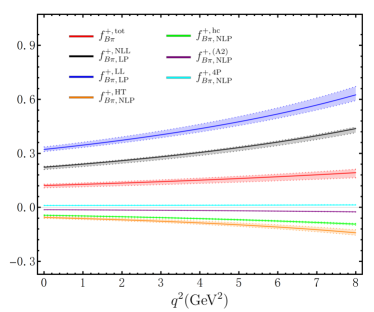
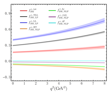
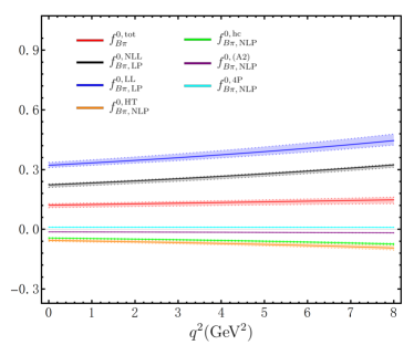
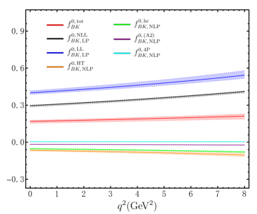
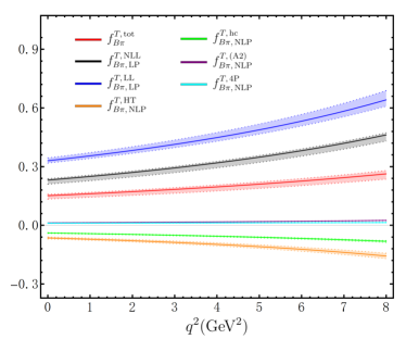
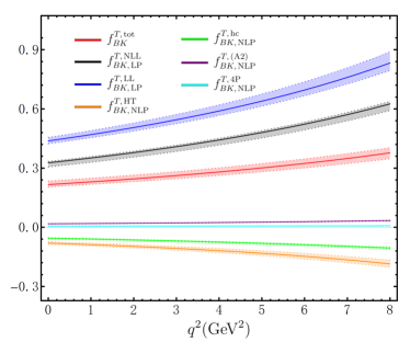
Figure 3: Breakdown of the distinct dynamical mechanisms contributing to the semileptonic $B\to\pi\ell\bar{\nu}_{\ell}$ form factors (left panel) and to the electroweak penguin $B\to K\nu_{\ell}\bar{\nu}_{\ell}$ decay form factors (right panel) in the kinematic region $0\leq q^{2}\leq 8\,{\rm GeV^{2}}$ from the updated LCSR computations with the HQET bottom-meson distribution amplitudes, where the perturbative uncertainties due to the variations of both the hard and hard-collinear matching scales are indicated by the individual error bands.

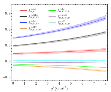
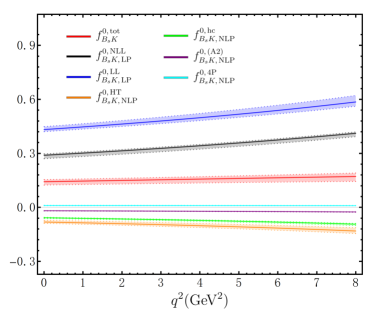
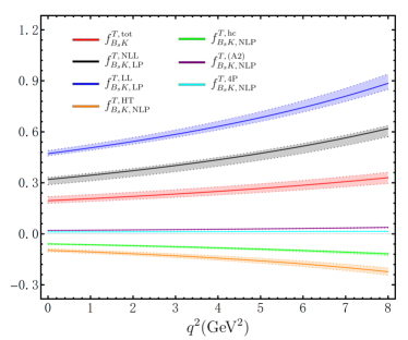
Figure 4: Breakdown of the distinct dynamical mechanisms contributing to the semileptonic $B_{s}\to K\ell\bar{\nu}_{\ell}$ form factors in the kinematic region $0\leq q^{2}\leq 8\,{\rm GeV^{2}}$ from the updated LCSR computations with the HQET bottom-meson distribution amplitudes, where the perturbative uncertainties due to the variations of both the hard and hard-collinear matching scales are indicated by the individual error bands.

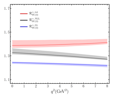
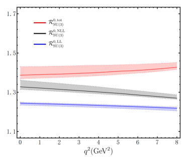
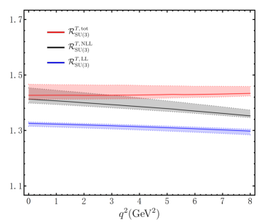
Figure 5: Theory predictions for the SU(3)-flavour symmetry breaking effects between the semileptonic $B\to\pi$ and $B\to K$ form factors from the updated SCET sum rules with the bottom-meson distribution amplitudes at the twist-six accuracy, where the perturbative uncertainties due to the variations of both the hard and hard-collinear matching scales are indicated by the individual error bands.

We are now in a position to investigate the SU(3)-flavour symmetry breaking effects between the exclusive $B\to\pi$ and $B\to K$ form factors, on the basis of the established SCET sum rules with the bottom-meson distribution amplitudes up to the twist-six accuracy, by introducing further the following quantities [35, 37]

$${\cal R}_{\rm SU(3)}^{i}(q^{2})=\left[f_{B\to K}^{i}(q^{2})\right]:\left[f_{B\to\pi}^{i}(q^{2})\right]\,,\qquad({\rm with}\,\,i=+,\,0,\,T)\,.$$ (112)

In our theoretical framework such flavour-symmetry violations arise from the apparent discrepancies in the light-quark masses, in the light-flavour hadron masses, in the leptonic decay constants $f_{\pi}$ and $f_{K}$, in the threshold parameters for the pion and kaon channels, and finally in the nonperturbative quark-condensate densities $\langle\bar{u}u\rangle$ and $\langle\bar{s}s\rangle$. It can be observed from Figure 5 that the leading-power LCSR predictions for the SU(3)-flavour symmetry breaking effects give rise to numerically ${\cal O}(30\,\%)$ for the two ratios ${\cal R}_{\rm SU(3)}^{+,\,0}$ and ${\cal O}(40\,\%)$ for the tensor-form-factor ratio ${\cal R}_{\rm SU(3)}^{T}$ in the large recoil region. In particular, the newly determined subleading-power contributions from the same LCSR method can only bring about the insignificant numerical impacts on the SU(3)-flavour symmetry violating effects (see [37] for the analogous observation for the exclusive semileptonic $B\to V\ell\bar{\nu}_{\ell}$ form factors). It is worthwhile mentioning that we have not taken into account the remaining sources of the SU(3)-flavour symmetry breaking effects due to the electromagnetic corrections and the systematic uncertainties owing to the parton-hadron duality approximation.

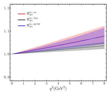
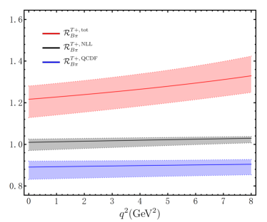
Figure 6: Theory predictions for the large-recoil symmetry breaking corrections between the exclusive $B\to\pi$ form factors from the updated SCET sum rules with the bottom-meson distribution amplitudes at the twist-six accuracy. For a comparison, we further display the numerical results from the QCD factorization approach with the so-called physical form factor scheme [90] by taking the light-meson LCSR computation of the vector form factor $f_{B\pi}^{+}(q^{2})$ [140] as the fundamental theory input.

We proceed to explore the celebrated large-recoil symmetry breaking effects between the exclusive heavy-to-light bottom-meson decay form factors due to the higher-order perturbative corrections and the intricate subleading-power corrections in the $\Lambda_{\rm QCD}/m_{b}$ expansion. In order to facilitate the straightforward comparison with the theory predictions from the QCD factorization approach, it proves convenient to investigate the two particular form-factor ratios for the semileptonic $B\to\pi\ell\bar{\nu}_{\ell}$ and $B\to\pi\ell\bar{\ell}$ decay processes [90, 35]

$${\cal R}_{B\pi}^{0+}(q^{2})=\left({m_{B}\over n\cdot p}\right)\,\frac{f_{B\pi}^{0}(q^{2})}{f_{B\pi}^{+}(q^{2})}\,,\qquad{\cal R}_{B\pi}^{T+}(q^{2})=\left({m_{B}\over m_{B}+m_{\pi}}\right)\,\frac{f_{B\pi}^{T}(q^{2})}{f_{B\pi}^{+}(q^{2})}\,.$$ (113)

It is interesting to notice that the NLL resummation improved LCSR predictions for the two quantities ${\cal R}_{B\pi}^{0+}$ and ${\cal R}_{B\pi}^{T+}$ are in reasonable agreement with the QCD factorization computations at the leading-power accuracy. On the contrary, confronting our numerical results for the form-factor ratio ${\cal R}_{B\pi}^{T+}$ from the bottom-meson LCSR method including four different classes of the NLP corrections with the counterpart predictions from QCD factorization reveal an intriguing tension on both the magnitude and sign of the large-recoil symmetry breaking corrections as displayed in Figure 6. Inspecting the individual terms in the obtained subleading-power sum rules (76) indicates that the emerged discrepancies between the two different QCD calculations stem from the newly determined NLP contribution of the power-suppressed ${\rm SCET_{I}}$ current $J^{\rm(A2)}$ with the LCSR method as collected in (52) explicitly, which has not been included in the numerical exploration of the current QCD factorization framework [90]. As a consequence, it becomes more and more demanding to construct the appropriate perturbative factorization formula for this NLP matrix element directly with the modern effective-field-theory technique.

Apparently, we can only establish the soft-collinear factorization formulae for the desired vacuum-to-$B$-meson correlation functions (2) at small and intermediate momentum transfers, $0\leq q^{2}\leq q_{\rm cut}^{2}$, where the practical choice of $q_{\rm cut}^{2}$ varies between $8\,{\rm GeV^{2}}$ and $10\,{\rm GeV^{2}}$ numerically. We are therefore required to extrapolate the bottom-meson LCSR computations of the semileptonic $B_{d,s}\to\pi,K$ form factors towards the large momentum transfer $q^{2}$ by applying the $z$-series parametrization based upon the positivity and analyticity properties of these transition form factors [143, 144, 145]. Adopting the conformal transformation [74, 76, 75]

$$z(q^{2},t_{0})=\frac{\sqrt{t_{+}-q^{2}}-\sqrt{t_{+}-t_{0}}}{\sqrt{t_{+}-q^{2}}+\sqrt{t_{+}-t_{0}}}\,,$$ (114)

with the threshold parameter $t_{+}\equiv\left[m_{B}+m_{\pi(K)}\right]^{2}$ for the exclusive semileptonic $b\to u(s)$ transitions, enables us to map the complex cut $q^{2}$-plane onto the unit disk $|z(q^{2},t_{0})|\leq 1$. On the other hand, the free parameter $t_{0}<t_{+}$ corresponds to the value of $q^{2}$ mapping onto the origin in the $z$-plane, namely $z(t_{0},t_{0})=0$. In order to maximally reduce the interval of $z$ obtained after mapping (114) of the semileptonic domain $q^{2}\in\left[0,\,(m_{B_{q^{\prime}}}-m_{M})^{2}\right]$, the auxiliary parameter $t_{0}$ can be customarily taken as

$$t_{0}=t_{+}-\sqrt{t_{+}\,(t_{+}-t_{-})}\,,\qquad t_{-}=(m_{B_{q^{\prime}}}-m_{M})^{2}\,.$$ (115)

following closely the comprehensive discussions presented in [16]. Taking into account further the asymptotic behaviours of the vector form factors near threshold due to the angular momentum conservation implies the simplified series expansion originally proposed in [76] (see [146, 147] for an alternative parametrization)

$$f_{B_{q^{\prime}}M}^{+}(q^{2}) = \frac{1}{1-q^{2}/m_{B_{q}^{\ast}}^{2}}\,\sum_{k=0}^{N-1}\,b_{k}^{+}\,\left[z(q^{2},t_{0})^{k}-(-1)^{k-N}\,{k\over N}\,z(q^{2},t_{0})^{N}\right]\,,$$ (116)

where the lowest bottom-meson $B_{d}^{\ast}$ ($B_{s}^{\ast}$) is expected to be the only resonance of the $J^{P}=1^{-}$ channel below the $B\pi$ ($BK$) production region. It is evident from the BCL parametrization (116) that the well-known scaling behaviour $f_{B_{q^{\prime}}M}^{+}(q^{2})\sim 1/q^{2}$ at $|q^{2}|\to\infty$ from the perturbative QCD analysis [148] is indeed fulfilled. For the practical purpose, we will truncate the $z$-series expansion at $N=3$ in the subsequent fitting program.

Along the same vein, we can proceed to parameterize the remaining form factors by adjusting the overall pole functions appropriately and by dropping out the near-threshold constraints for the scalar transition form factors

$$f_{B_{(s)}\pi(K)}^{0}(q^{2}) = \,\sum_{k=0}^{N-1}\,b_{k}^{0}\,\,z(q^{2},t_{0})^{k}\,,\qquad f_{BK}^{0}(q^{2})=\frac{1}{1-q^{2}/m_{B_{s}^{\ast}(0+)}^{2}}\,\sum_{k=0}^{N-1}\,b_{k}^{0}\,\,z(q^{2},t_{0})^{k}\,,$$

$$f_{B_{q^{\prime}}M}^{T}(q^{2}) = \frac{1}{1-q^{2}/m_{B_{q}^{\ast}}^{2}}\,\sum_{k=0}^{N-1}\,b_{k}^{T}\,\left[z(q^{2},t_{0})^{k}-(-1)^{k-N}\,{k\over N}\,z(q^{2},t_{0})^{N}\right]\,.$$ (117)

The very disappearance of the pole factors in the above-mentioned parameterizations of the two particular form factors $f_{B\pi}^{0}(q^{2})$ and $f_{B_{s}K}^{0}(q^{2})$ can be attributed to the fact that the low-lying bottom-resonance in the $J^{P}=0^{+}$ channel with the predicted mass $m_{B^{\ast}(0+)}=(5627\pm 35)\,{\rm MeV}$ [113] turns out to be located above the $B\pi$ production threshold $m_{B}+m_{\pi}=(5419\pm 0.12)\,{\rm MeV}$ [89]. By contrast, the low-lying bottom-meson resonance in the BCL parametrization (117) for the scalar form factor $f_{BK}^{0}(q^{2})$, with the estimated mass $m_{B_{s}^{\ast}(0+)}=(5718\pm 35)\,{\rm MeV}$ from the heavy-hadron chiral perturbation theory [113], appears to be somewhat below the particle-pair production threshold $m_{B}+m_{K}=(5773\pm 0.12)\,{\rm MeV}$ [89]. For convenience, we have also summarized the relevant resonance masses employed in our $z$-parametrization fits in Table 1.

$B\to\pi$   Form Factors		Correlation Matrix
Parameters	Values	$b_{0}^{+}$	$b_{1}^{+}$	$b_{2}^{+}$	$b_{0}^{0}$	$b_{1}^{0}$	$b_{0}^{T}$	$b_{1}^{T}$	$b_{2}^{T}$
$b_{0}^{+}$	$0.404(13)$	$1$	$0.276$	$-0.446$	$0.291$	$0.164$	$0.583$	$0.266$	$-0.24$
$b_{1}^{+}$	$-0.618(63)$		$1$	$-0.374$	$0.067$	$0.485$	$0.234$	$0.693$	$-0.193$
$b_{2}^{+}$	$-0.473(215)$			$1$	$0.108$	$0.157$	$-0.185$	$-0.185$	$0.592$
$b_{0}^{0}$	$0.496(19)$				$1$	$-0.226$	$0.318$	$0.06$	$0.018$
$b_{1}^{0}$	$-1.537(56)$					$1$	$0.04$	$0.431$	$0.165$
$b_{0}^{T}$	$0.396(15)$						$1$	$0.178$	$-0.423$
$b_{1}^{T}$	$-0.553(73)$							$1$	$-0.307$
$b_{2}^{T}$	$-0.248(235)$								$1$

Table 2: Theory predictions for the correlated $z$-series coefficients in the vector, scalar and tensor $B\to\pi$ form factors determined by fitting the BGL parametrization simultaneously against our LCSR results including a variety of the subleading-power corrections and the available lattice QCD data points from [4, 3, 7] with the preferred truncation $N=3$.

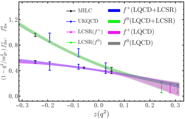
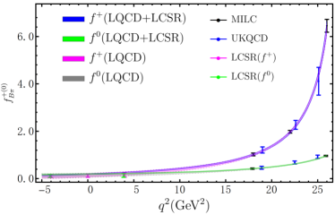
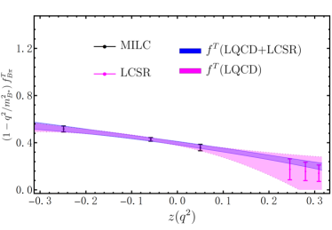
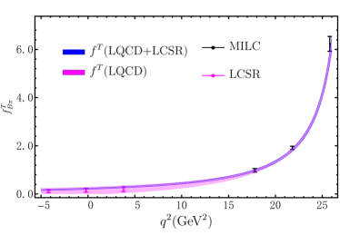
Figure 7: Theory predictions for the complete set of the semileptonic $B\to\pi$ form factors versus $z$ (left panel) and versus $q^{2}$ (right panel) in the entire kinematic region obtained by carrying out the combined BCL $z$-fit of the updated LCSR (from this work) and lattice QCD (from [4, 3, 7]) data points. We further display the yielding numerical results of these form factors by performing an alternative $z$-series fit against the “only lattice QCD” data points [4, 3, 7] exclusively for a comparison.

We are now prepared to determine the BCL series coefficients $b_{k}^{+,\,0,\,T}$ by performing the binned $\chi^{2}$ fit of the updated LCSR predictions for the bottom-meson decay form factors at three distinct kinematic points, namely $q^{2}=\left\{-4.0,\,0,\,4.0\right\}\,{\rm GeV^{2}}$, in combination with the available lattice data points in the higher-$q^{2}$ region. Enforcing the kinematic constraint between the vector and scalar form factors $f_{BM}^{+}(0)=f_{BM}^{0}(0)$ allows us further to derive the following exact relations between the expansion coefficients of our interest

$$b_{2}^{0} = 12.78\,\left(b_{0}^{+}-b_{0}^{0}\right)+3.482\,b_{1}^{+}+1.186\,b_{2}^{+}-3.575\,b_{1}^{0}\,,\qquad({\rm for}\,\,B\to\pi)$$

$$b_{2}^{0} = 24.06\,\left(b_{0}^{+}-b_{0}^{0}\right)+4.837\,b_{1}^{+}+1.136\,b_{2}^{+}-4.905\,b_{1}^{0}\,,\qquad({\rm for}\,\,B_{s}\to K)$$

$$b_{2}^{0} = 48.59\,\left(b_{0}^{+}-b_{0}^{0}\right)+6.923\,b_{1}^{+}+1.096\,b_{2}^{+}-6.971\,b_{1}^{0}\,.\qquad({\rm for}\,\,B\to K)$$ (118)

With regard to the lattice QCD results for the semileptonic $B\to\pi$ form factors, we can straightforwardly employ the synthetic data points of $f_{B\pi}^{+}(q^{2})$ and $f_{B\pi}^{0}(q^{2})$ at three representative values of $q^{2}=\left\{19.0,\,22.6,\,25.1\right\}\,{\rm GeV^{2}}$ with the full correlation matrices from the RBC/UKQCD Collaboration [4], by adopting $N_{f}=2+1$-flavour gauge-field ensembles with the domain-wall fermion action and Iwasaki gluon action. However, the FNAL/MILC Collaboration do not provide the yielding data points for the exclusive $B\to\pi$ form factors explicitly in their publications [3, 7], which present the outcome of the combined BCL fit to their data points with the truncation $N=3$ instead. Consequently, we will take advantage of the BCL fit results to generate the correlated synthetic data points of the three $B\to\pi$ form factors in the kinematic region $19.0\,{\rm GeV}^{2}\leq q^{2}\leq 26.4\,{\rm GeV}^{2}$. Carrying out the simultaneous fit of the conventional BCL parameterizations (116) and (117) to our LCSR pseudo data points as well as the lattice QCD data points gives rise to the desired intervals of the $z$-series coefficients and their correlation matrix for the semileptonic $B\to\pi$ form factors displayed in Table 2. Furthermore, we observe that this numerical fit yields a minimal $\chi^{2}=7.93$ for $14$ degrees of freedom in the fitting program, which corresponds to an excellent $p$-value of $89\,\%$ in turn. It has been verified manifestly that the fitted BCL coefficients fulfill the very dispersive bounds [76, 149] derived from the correlation functions of two flavour-changing currents with the aid of unitarity and crossing symmetry (see [150] for further discussions on the scaling behaviour of the sum of coefficients $\sum_{k=0}^{N}\left(b_{k}^{+}\right)^{2}$ in the heavy quark limit). In order to develop a transparent understanding towards the eventually predicted momentum-transfer dependence from interpolating the LCSR and lattice QCD results, we display the obtained numerical predictions for the three exclusive $B\to\pi$ form factors versus $z$ (left panel) and versus $q^{2}$ (right panel) in the entire kinematic region in Figure 7, where the counterpart predictions of these form factors from implementing an alternative $z$-expansion fit of the “only lattice QCD” data points [4, 3, 7] exclusively are further shown for the convenience. It is evident from this comparative exploration that including the newly derived LCSR data points at small momentum transfer in our fitting procedure will indeed be highly beneficial for improving the theory precision for all three $B\to\pi$ form factors in the kinematic regime $0.10\leq z\leq 0.31$ (namely, $q^{2}\in\left[-4.0,15.5\right]\,{\rm GeV^{2}}$) significantly. This interesting observation can be actually understood from the very fact that extrapolating the current lattice QCD results towards the lower $q^{2}$ region solely will bring about the more pronounced uncertainties for the form-factor shapes in comparison with the direct LCSR computations as already discussed in [4, 3, 7].

Additionally, it is instructive to compare our form-factor predictions from the combined BCL fit with the theoretical expectations from the heavy quark spin symmetry and the current algebra method. In the zero-recoil limit we can derive an interesting relation between the vector and scalar form factors up to the accuracy of ${\cal O}(\Lambda_{\rm QCD}^{2}/m_{b}^{2})$ [151]

$$\lim_{q^{2}\to m_{B_{q^{\prime}}}^{2}}\,\frac{f_{B_{q^{\prime}}M}^{+}(q^{2})}{f_{B_{q^{\prime}}M}^{0}(q^{2})}=\left(\frac{f_{B_{q}^{\ast}}}{f_{B_{q^{\prime}}}}\right)\,\left(1-{m_{M}^{2}\over m_{B_{q^{\prime}}}^{2}}\right)\,\left(\frac{\hat{g}_{\rm eff}}{1-q^{2}/m_{B_{q}^{\ast}}^{2}}\right)\,,$$ (119)

where the static coupling $\hat{g}_{\rm eff}$ entering the Lagrangian density of the heavy-hadron chiral perturbation theory is independent of the heavy quark mass [134]. We will adopt the nonperturbative determination of this low-energy constant from the NLO LCSR computations with the pion distribution amplitudes $\hat{g}_{\rm eff}=0.30\pm 0.02$ [152] (see also [153, 154] for the earlier analyses in the same framework). Moreover, we will employ the updated numerical results for the leptonic decay constants of the heavy-light vector mesons [116]

$$f_{B^{\ast}}=210^{+10}_{-12}\,{\rm MeV}\,,\qquad f_{B_{s}^{\ast}}=251^{+14}_{-16}\,{\rm MeV}\,,$$ (120)

based upon the standard method of the two-point QCD sum rules. We present the obtained numerical predictions for the form-factor ratio $\left[\left(1-q^{2}/m_{B_{q}^{\ast}}^{2}\right)\,f_{B_{q^{\prime}}M}^{+}(q^{2})\right]:\left[f_{B_{q^{\prime}}M}^{0}(q^{2})\right]$ from the combined $z$-expansion fitting program in the lower-recoil region in Figure 8, where the complementary predictions with uncertainties from the combination of heavy quark and chiral symmetries are further displayed explicitly for a comparison.

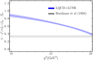
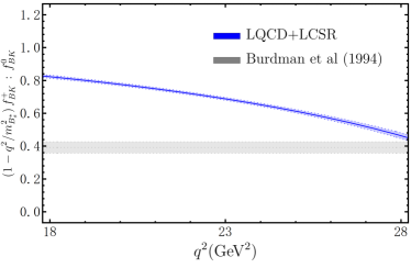
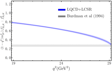
Figure 8: Theory predictions of the particular form-factor ratio $\left[\left(1-q^{2}/m_{B_{q}^{\ast}}^{2}\right)\,f_{B_{q^{\prime}}M}^{+}(q^{2})\right]:\left[f_{B_{q^{\prime}}M}^{0}(q^{2})\right]$ for the exclusive semileptonic $B_{d,s}\to\pi,K$ decays determined from the combined $z$-expansion fit against the LCSR and lattice QCD data points (blue bands) and from the theoretical expectations of the heavy quark spin symmetry and the current algebra technique at NLO in the $\Lambda/m_{b}$ expansion [151] (grey bands).

The heavy quark spin symmetry relation between the vector and tensor form factors in the low recoil region can be derived by exploring an exact operator identity on account of the QCD equations of motion for the quark fields

$$i\,\partial^{\nu}\left(\bar{q}\,i\,\sigma_{\mu\nu}\,b\right)=i\,\,\partial_{\mu}\left(\bar{q}\,b\right)\,-(m_{b}+m_{q})\,\bar{q}\,\gamma_{\mu}\,b\,-2\,\left(\bar{q}\,i\,\overleftarrow{D}_{\mu}\,b\right)\,,$$ (121)

and by employing the Lorentz decomposition for the subleading heavy-to-light HQET matrix element of the dimension-four operator [155, 156]

$$\langle M(p)|\bar{q}\,i\,\overleftarrow{D}_{\mu}\,h_{v}|\bar{B}(p_{B})\rangle=\delta_{+}(q^{2})\,(2\,p+q)_{\mu}+\delta_{-}(q^{2})\,q_{\mu}\,.$$ (122)

Performing the conventional matching procedure ${\rm QCD}\to{\rm HQET}$ for the emerged flavour-changing weak currents in the previous identity (121)

$$\bar{q}\,\gamma_{\mu}\,b \to C_{0}^{(v)}(\mu)\,\,\bar{q}\,\gamma_{\mu}\,h_{v}\,+\,C_{1}^{(v)}(\mu)\,\,\bar{q}\,v_{\mu}\,h_{v}\,+\,\left({1\over 2\,m_{b}}\right)\,\bar{q}\,\gamma_{\mu}\,i\,\not{D}\,h_{v}+...\,,$$

$$\bar{q}\,i\,\overleftarrow{D}_{\mu}\,b \to D_{0}^{(v)}(\mu)\,\overline{m}_{b}(\mu)\,\,\bar{q}\,\gamma_{\mu}\,h_{v}+D_{1}^{(v)}(\mu)\,\overline{m}_{b}(\mu)\,\,\bar{q}\,v_{\mu}\,h_{v}+\bar{q}\,i\,\overleftarrow{D}_{\mu}\,h_{v}+...\,,$$ (123)

we can readily derive an improved Isgur-Wise relation between the semileptonic bottom-meson decay form factors in the small recoil region [155, 157]

$$\frac{f_{B_{q^{\prime}}M}^{T}(q^{2})}{f_{B_{q^{\prime}}M}^{+}(q^{2})}=\frac{m_{B_{q^{\prime}}}(m_{B_{q^{\prime}}}+m_{M})}{q^{2}}\left[{\cal C}_{\rm T+}(\mu)+\left({2\over m_{B_{q}^{\prime}}}\right)\frac{\delta_{+}(q^{2})}{f_{B_{q^{\prime}}M}^{+}(q^{2})}\right]+{\cal O}\left(\left({\Lambda_{\rm QCD}\over m_{b}}\right)^{2}\right),\hskip 22.76228pt$$ (124)

The short-distance matching function ${\cal C}_{\rm T+}$ can be evidently expressed in terms of the Wilson coefficients of the HQET currents [156]

$${\cal C}_{\rm T+}(\mu)=\left[1+\frac{2\,D_{0}^{(v)}(\mu)}{C_{0}^{(v)}(\mu)}\right]\,\frac{\overline{m}_{b}(\mu)}{m_{B_{q^{\prime}}}}\,,$$ (125)

where the analytical expressions of $C_{0}^{(v)}$ and $D_{0}^{(v)}$ at the one-loop accuracy can be written as

$$C_{0}^{(v)}(\mu) = 1-{\alpha_{s}(\mu)\,C_{F}\over 4\,\pi}\,\left(3\,\ln{\mu\over m_{b}}+4\right)+{\cal O}(\alpha_{s}^{2})\,,$$

$$D_{0}^{(v)}(\mu) = 0+{\alpha_{s}(\mu)\,C_{F}\over 4\,\pi}\,\left(2\,\ln{\mu\over m_{b}}+2\right)+{\cal O}(\alpha_{s}^{2})\,.$$ (126)

Applying further the HQET equation of motion for the effective field $h_{v}$ enables us to derive an important constraint between the two subleading form factors [155]

$$(m_{B_{q^{\prime}}}+v\cdot p)\,\delta_{+}(q^{2})+(m_{B_{q^{\prime}}}-v\cdot p)\,\delta_{-}(q^{2})=0\,.$$ (127)

Evaluating the effective matrix element (122) with the aid of the heavy-hadron chiral perturbation theory at the lowest order in the $v\cdot p/\Lambda_{\rm CSB}$ expansion (with the notation $\Lambda_{\rm CSB}$ characterizing the chiral-symmetry-breaking scale) leads to the model-independent prediction

$$\delta_{+}(q^{2})-\delta_{-}(q^{2})=\frac{2\,\bar{\Lambda}\,f_{B_{q^{\prime}}}}{3\,f_{M}}\,\left(\frac{\hat{g}_{\rm eff}}{1-q^{2}/m_{B_{q}^{\ast}}^{2}}\right)\,,$$ (128)

where the hadronic parameter $\bar{\Lambda}$ stands for the “effective mass” of the bottom-meson state as previously defined in (29). It is then straightforward to determine the desired soft function $\delta_{+}(q^{2})$ dictating the considered form-factor ratio (124)

$$\delta_{+}(q^{2})=\frac{\bar{\Lambda}\,f_{B_{q^{\prime}}}}{3\,f_{M}}\,\left({m_{B_{q}^{\prime}}^{2}+q^{2}\over 2\,m_{B_{q}^{\prime}}^{2}}\right)\,\left(\frac{\hat{g}_{\rm eff}}{1-q^{2}/m_{B_{q}^{\ast}}^{2}}\right)\,.$$ (129)

We present the yielding theory predictions for the very form-factor ratio $\left[q^{2}\,f_{B_{q^{\prime}}M}^{T}(q^{2})\right]:\left[m_{B_{q^{\prime}}}(m_{B_{q^{\prime}}}+m_{M})\,f_{B_{q^{\prime}}M}^{+}(q^{2})\right]$ from fitting the BCL $z$-series expansion against the LCSR and lattice QCD data points in the lower-recoil region in Figure 9, where the theoretical expectations from the improved Isgur-Wise relation (124) in the soft final-state meson approximation in virtue of the heavy quark spin symmetry are further shown for a numerical comparison.

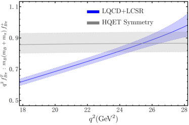
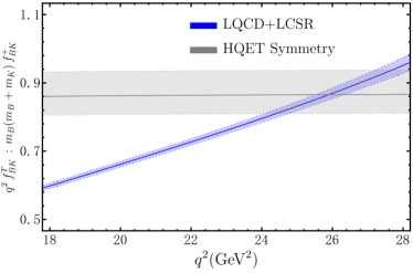
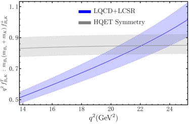
Figure 9: The low-recoil theory predictions for the intriguing form-factor ratio $\left[q^{2}\,f_{B_{q^{\prime}}M}^{T}(q^{2})\right]:\left[m_{B_{q^{\prime}}}\,(m_{B_{q^{\prime}}}+m_{M})\,f_{B_{q^{\prime}}M}^{+}(q^{2})\right]$ for the exclusive semileptonic $B_{d,s}\to\pi,K$ decay processes determined from the combined BCL $z$-series expansion fitting against both the LCSR and lattice QCD data points (blue bands) and from the theoretical expectations of the improved Isgur-Wise relation (124) at the NLP accuracy due to the combination of heavy quark and chiral symmetries (grey bands) [155, 156].

Subsequently, we proceed to carry out the combined BCL $z$-expansion fitting of the semileptonic $B\to K$ form factors against the newly determined LCSR data points at three representative values of $q^{2}=\left\{-4.0,\,0,\,4.0\right\}\,{\rm GeV^{2}}$, in combination with the small-recoil lattice QCD results achieved with the three-flavor gauge-field ensembles generated by the MILC Collaboration [14] (employing further the Sheikholeslami-Wohlert (SW) action with the Fermilab interpretation for the bottom quark) as well as obtained for the first time with $N_{f}=2+1+1$ gluon field ensembles [15] (in the meanwhile adopting the highly improved staggered quark (HISQ) formalism for all valence and sea quarks developed by the HPQCD Collaboration). Since neither of these lattice collaborations provide explicitly the resulting physical data points for the three exclusive $B\to K$ form factors in their publications, we are then required to generate the correlated synthetic data points in the kinematic region $16.8\,{\rm GeV}^{2}\leq q^{2}\leq 22.9\,{\rm GeV}^{2}$ from their BCL expansion fit results with the truncation $N=3$ as documented in [14, 15]. We remark in passing that the HPQCD Collaboration actually adopted the so-called “modified $z$-expansion” strategy by simultaneously extrapolate the obtained lattice simulation data to the physical light-quark masses and zero lattice spacing, and to interpolate their lattice results in the momentum transfer (see [16] for more technical discussions on this alternative approach). Implementing now the binned $\chi^{2}$ fit for both the LCSR and lattice simulation results with the standard BCL parametrization (116) and (117) leads to our final numerical predictions of the eight form-factor parameters (with their correlation matrix) indispensable for the theory description of the electroweak penguin $B\to K\ell\bar{\ell}$ decays [107, 108] as summarized in Table 3. We further observe that our BCL expansion fit brings about a minimal $\chi^{2}=14.12$ for $16$ degrees of freedom in the fitting procedure, thus corresponding to an encouraging $p$-value of $59\,\%$ numerically. Adopting the tabulated $z$-series coefficients $b_{k}^{+,0,T}$ allows us to predict the desired momentum-transfer dependence for the three semileptonic $B\to K$ form factors versus $z$ (left panel) and versus $q^{2}$ (right panel) in the entire kinematic region in Figure 10, where we also display the corresponding theory predictions from performing an independent $z$-series fitting to the “only lattice QCD” data points [14, 15] exclusively for the convenience. It turns out that the rather remarkable precision for the whole lattice data points at high momentum transfer from both the FNAL/MILC Collaboration [14] (with the total uncertainties, including both statistical and systematic errors, less than $4.0\,\%$ for all the three $B\to K$ form factors) and the HPQCD Collaboration [15] (with the uncertainties below $\{2.0\,\%,4.0\,\%,5.5\,\%\}$ for the three form factors $\{f_{BK}^{+},\,f_{BK}^{0},\,f_{BK}^{T}\}$ in consequence) makes it challenging to carry out the combined BCL $z$-series fit with high quantity, by simultaneously accommodating the achieved LCSR predictions at low momentum transfer within the individual $1.0\,\sigma$ intervals (albeit with the very sizeable theory uncertainties of the order of $50\,\%$). Actually, this intriguing observation can be attributed to the very fact that our updated LCSR computations with the bottom-meson distribution amplitudes will bring about the strongly correlated numerical results for the exclusive $B\to K$ form factors at the different kinematic points (despite of the quite uncertain central values as explained above) in the large hadronic recoil region, which exhibit the delicacy tension with the extrapolated lattice QCD predictions with the extraordinary high accuracy in the low recoil region. In this respect, it would be in high demand to deepen further our understanding, on the one hand, towards the momentum dependence of the HQET bottom-meson distribution amplitudes $\phi_{B}^{\pm}(\omega,\mu_{0})$ at the renormalization scale $\mu_{0}=1.0\,{\rm GeV}$ from the first field-theoretical principles on the bottom-meson LCSR aspect, and on the other hand, towards the unquantified systematic uncertainties of the lattice simulation method (for instance, several potential concerns with the “modified $z$-expansion” proposal as previously discussed in [16]).

Furthermore, we confront the combined BCL expansion fit results for the two particular form-factor ratios (119) and (124) at high momentum transfer with the counterpart model-independent predictions from the combination of the heavy quark spin symmetry and the current algebra technique in Figures 8 and 9. Generally, the resulting BCL $z$-fit predictions for the considered low-recoil symmetry breaking corrections appear to be in reasonable agreement with the theoretical expectations from the HQET symmetry relations at the unphysical kinematic point $q^{2}=27.9\,{\rm GeV^{2}}$ within the obtained uncertainties. By contrast, our BCL fit result for the scalar form-factor ratio at the zero-recoil limit differs from the counterpart prediction with the heavy quark symmetry and the soft-kaon approximation by an enormous amount of ${\cal O}(50\,\%)$, thus confirming the previous lattice simulation results from the FNAL/MILC Collaboration [14]. We are then led to conclude immediately that employing the derived low-recoil symmetry relations for the exclusive $B\to K\ell\bar{\ell}$ phenomenological applications could result in the substantial derivations from the direct QCD predictions due to the numerically pronounced NLP corrections in the heavy quark expansion.

$B\to K$   Form Factors		Correlation Matrix
Parameters	Values	$b_{0}^{+}$	$b_{1}^{+}$	$b_{2}^{+}$	$b_{0}^{0}$	$b_{1}^{0}$	$b_{0}^{T}$	$b_{1}^{T}$	$b_{2}^{T}$
$b_{0}^{+}$	$0.465(8)$	$1$	$-0.035$	$-0.494$	$0.711$	$0.283$	$0.744$	$0.017$	$-0.281$
$b_{1}^{+}$	$-0.925(53)$		$1$	$-0.034$	$0.160$	$0.831$	$-0.111$	$0.691$	$-0.056$
$b_{2}^{+}$	$-0.355(257)$			$1$	$-0.038$	$0.166$	$-0.299$	$-0.099$	$0.533$
$b_{0}^{0}$	$0.290(4)$				$1$	$0.422$	$0.594$	$0.061$	$-0.015$
$b_{1}^{0}$	$0.246(38)$					$1$	$0.141$	$0.595$	$0.14$
$b_{0}^{T}$	$0.479(10)$						$1$	$-0.023$	$-0.283$
$b_{1}^{T}$	$-0.759(74)$							$1$	$0.305$
$b_{2}^{T}$	$-0.479(324)$								$1$

Table 3: Theory predictions for the correlated $z$-series coefficients in the vector, scalar and tensor $B\to K$ form factors determined by fitting the BGL parametrization simultaneously against our LCSR results including a variety of the subleading-power corrections and the available lattice QCD data points from [14, 15] with the preferred truncation $N=3$.

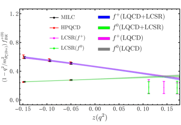
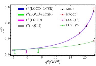
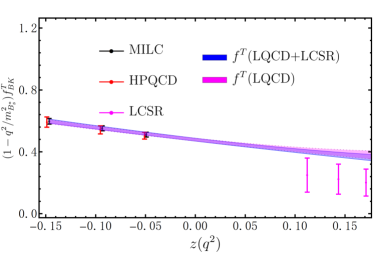
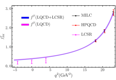
Figure 10: Theory predictions for the complete set of the semileptonic $B\to K$ form factors versus $z$ (left panel) and versus $q^{2}$ (right panel) in the entire kinematic region obtained by carrying out the combined BCL $z$-fit of the updated LCSR (from this work) and lattice simulation (from [14, 15]) data points. We further display the yielding numerical results of these essential form factors by performing an independent $z$-series fit against the “only lattice QCD” data points [14, 15] exclusively for an instructive comparison.

Along the same vein, we will continue to perform the combined BCL expansion fitting of the semileptonic $B_{s}\to K$ form factors against our improved LCSR predictions and the available lattice results for the vector and scalar form factors [4, 8, 11] simultaneously. On account of the very absence of the lattice simulation results for the tensor form factor, we prefer to take advantage of the determined LCSR data points for $f_{B_{s}K}^{T}(q^{2})$ at five representative values of $q^{2}=\left\{-8.0,\,-4.0,\,0,\,4.0,\,8.0\right\}\,{\rm GeV^{2}}$, while adopting the large-recoil LCSR predictions for the vector and scalar form factors $f_{B_{s}K}^{+,\,0}(q^{2})$ at three distinct kinematic points of $q^{2}=\left\{-4.0,\,0,\,4.0\right\}\,{\rm GeV^{2}}$ as the same as before. While the RBC/UKQCD Collaboration [4] provides explicitly the synthetic data points of $f_{B_{s}K}^{+}(q^{2})$ and $f_{B_{s}K}^{0}(q^{2})$ at three representative values of $q^{2}=\left\{17.6,\,20.8,\,23.4\right\}\,{\rm GeV^{2}}$ with the normalized statistical and systematic correlation matrices, both the HPQCD Collaboration [8] and the FNAL/MILC Collaboration [11] only provide their BCL $z$-fit results for the form-factor shape parameters with the truncations $N=3$ and $N=4$, respectively. Consequently, we are then required to produce the necessary lattice data points for $f_{B_{s}K}^{+,\,0}(q^{2})$ in the kinematic region $17.0\,{\rm GeV}^{2}\leq q^{2}\leq 23.7\,{\rm GeV}^{2}$ in order to utilize the complete information of the lattice QCD fits from [8, 11]. Performing now the combined BCL fit against both our LCSR predictions in the large recoil region and the yielding lattice simulation data points in the low recoil region gives rise to the final predictions for the $z$-expansion coefficients (with their correlation matrix) for the three semileptonic $B_{s}\to K$ form factors as collected in Table 4. In addition, our numerical fit leads to a slightly larger number of $\chi^{2}=28.58$ for $19$ degrees of freedom in the fitting program. Unsurprisingly, the obtained BCL fit results for the three coefficients $b_{0,1,2}^{T}$ in Table 4 turn out to be more uncertain compared with the corresponding predictions for the $z$-expansion parameters of the tensor $B\to\pi$ form factor collected in Table 2, due to the unavailable lattice data points for the form factor $f_{B_{s}K}^{T}(q^{2})$ at large momentum transfer. Under such circumstance, achieving the lattice simulation determination for the very tensor form factor $f_{B_{s}K}^{T}(q^{2})$ at high $q^{2}$ will be evidently crucial to pin down the current theory uncertainties from the BCL extrapolation of the LCSR results, thus providing the fundamental ingredient for the model-independent description of the exclusive electroweak penguin $\bar{B}_{s}\to\bar{K}^{0}\ell\bar{\ell}$ decays. Employing the tabulated $z$-series coefficients $b_{k}^{+,0,T}$ further enables us to predict the desired momentum-transfer dependence for the exclusive $B_{s}\to K$ form factors versus $z$ (left panel) and versus $q^{2}$ (right panel) in the entire kinematic region in Figure 11, where we also display the alternative BCL fit results for the vector and scalar form factors with the “only lattice QCD” data points [4, 8, 11] exclusively. In the light of the high-precision lattice data points for $f_{B_{s}K}^{+,\,0}(q^{2})$ at small hadronic recoil from the RBC/UKQCD Collaboration [4] (with the total uncertainties below $\left\{6.2\,\%,\,7.1\,\%\right\}$ for the vector and scalar form factors, respectively), from HPQCD Collaboration [8] (with the combined uncertainties below $\left\{5.0\,\%,\,6.0\,\%\right\}$ for the two form factors $\{f_{B_{s}K}^{+},\,f_{B_{s}K}^{0}\}$ in consequence) and from the FNAL/MILC Collaboration [11] (with the uncertainties less than $3.0\,\%$ for both the two form factors), the resulting theory benefits from the combined BCL $z$-expansion fit to both the LCSR and lattice simulation results consist in the rather moderate improvements (at the level of ${\cal O}(20\,\%)$ numerically) of the large-recoil form factor predictions on the counterpart BCL fitting procedure with the “only lattice QCD” data points.

We proceed to compare the combined BCL expansion fitting predictions for the two form-factor ratios (119) and (124) in the low recoil region with the corresponding model-independent computations based upon the combination of heavy quark and chiral symmetries in Figures 8 and 9. We can draw an analogous conclusion (as previously observed in the context of the $B\to K$ form factors) that the derived HQET symmetry relations for the exclusive $B_{s}\to K$ form factors appear to be well respected at the unphysical kinematic point $q^{2}=28.8\,{\rm GeV^{2}}$ within the theory uncertainties. Apparently, our numerical result for the particular form-factor ratio $\left[q^{2}\,f_{B_{s}K}^{T}(q^{2})\right]:\left[m_{B_{s}}(m_{B_{s}}+m_{K})\,f_{B_{s}K}^{+}(q^{2})\right]$ suffers from the more pronounced theory uncertainty as displayed in Figure 9, due to the relatively less precise BCL-fitting prediction for the tensor form factor $f_{B_{s}K}^{+}(q^{2})$. Moreover, the very low-recoil symmetry breaking correction to the scalar form-factor ratio $\left[\left(1-q^{2}/m_{B^{\ast}}^{2}\right)\,f_{B_{s}K}^{+}(q^{2})\right]:\left[f_{B_{s}K}^{0}(q^{2})\right]$ at the maximal momentum transfer turns out to be even greater than the counterpart theory predictions for both the semileptonic $B\to\pi,K$ decay form-factor ratios as shown in Figure 8.

$B_{s}\to K$   Form Factors		Correlation Matrix
Parameters	Values	$b_{0}^{+}$	$b_{1}^{+}$	$b_{2}^{+}$	$b_{0}^{0}$	$b_{1}^{0}$	$b_{0}^{T}$	$b_{1}^{T}$	$b_{2}^{T}$
$b_{0}^{+}$	$0.373(10)$	$1$	$0.202$	$-0.294$	$0.653$	$0.135$	$0.422$	$-0.277$	$0.103$
$b_{1}^{+}$	$-0.731(41)$		$1$	$0.075$	$0.255$	$0.683$	$0.488$	$-0.301$	$0.092$
$b_{2}^{+}$	$-0.473(146)$			$1$	$0.099$	$0.366$	$0.215$	$-0.121$	$0.025$
$b_{0}^{0}$	$0.443(10)$				$1$	$-0.024$	$0.407$	$-0.268$	$0.100$
$b_{1}^{0}$	$-1.427(45)$					$1$	$0.433$	$-0.262$	$0.075$
$b_{0}^{T}$	$0.437(46)$						$1$	$-0.835$	$0.550$
$b_{1}^{T}$	$-0.900(167)$							$1$	$-0.914$
$b_{2}^{T}$	$0.091(172)$								$1$

Table 4: Theory predictions for the correlated $z$-series coefficients in the vector, scalar and tensor $B_{s}\to K$ form factors determined by fitting the BGL parametrization simultaneously against our LCSR results including a variety of the subleading-power corrections and the available lattice QCD data points from [4, 8, 11] with the preferred truncation $N=3$.

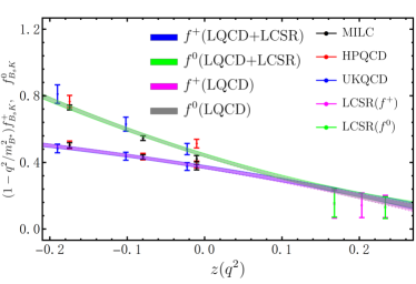
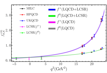
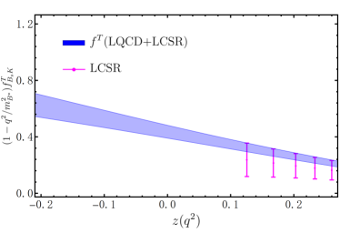
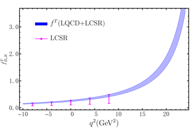
Figure 11: Theory predictions for the complete set of the semileptonic $B_{s}\to K$ form factors versus $z$ (left panel) and versus $q^{2}$ (right panel) in the entire kinematic region obtained by carrying out the combined BCL $z$-fit of the updated LCSR (from this work) and lattice simulation (merely for the two form factors $f_{B_{s}K}^{+,\,0}(q^{2})$ from [4, 8, 11]) data points. We further display the yielding numerical results for the vector and scalar form factors by performing an independent $z$-series fit against the “only lattice QCD” data points [4, 8, 11] exclusively for the illustration purpose.

4.3 Phenomenological analysis of the $B_{(s)}\to\pi(K)\ell\bar{\nu}_{\ell}$ observables

Having at our disposal the combined BCL $z$-fit results for the exclusive $B\to\pi,K$ form factors, we are now prepared to explore their phenomenological implications on the semileptonic $B_{(s)}\to\pi(K)\ell\bar{\nu}_{\ell}$ decay observables constructed from the corresponding full angular distributions, such as the differential branching fractions, the normalized forward-backward asymmetries, the new-physics (NP) sensitive “flat terms” (vanishing in the massless lepton limit in the SM), and the lepton-flavour universality ratios, the lepton polarization asymmetries. In particular, the ever-increasing precision measurements on the binned $q^{2}$ distributions for the golden exclusive $B\to\pi\ell\bar{\nu}_{\ell}$ (with $\ell=e,\,\mu$) decay processes from the BaBar Collaboration [62, 63], the Belle Collaboration [64, 65] as well as the Belle II [66] Collaboration enable us to further extract the desired CKM matrix element $|V_{ub}|$ straightforwardly in combination with our improved determination of the vector form factor $f_{B\pi}^{+}(q^{2})$ in the entire kinematic regime. In order to achieve this goal, we first present the explicit expression for the full differential decay distribution of $B_{q^{\prime}}\to M\ell\bar{\nu}_{\ell}$ with respect to the two kinematic variables $q^{2}$ and $\cos\theta_{\ell}$ (dropping out the very intricate but numerically subdominant electromagnetic correction)

$$\frac{d^{2}\Gamma(B_{q^{\prime}}\to M\ell\bar{\nu}_{\ell})}{dq^{2}\,d\cos\theta_{\ell}}=a_{\theta_{\ell}}(q^{2})+b_{\theta_{\ell}}(q^{2})\,\cos\theta_{\ell}+c_{\theta_{\ell}}(q^{2})\,\cos^{2}\theta_{\ell}\,,$$ (130)

where the three $q^{2}$-dependent angular coefficient functions are given by [158]

$$a_{\theta_{\ell}}(q^{2}) = {\cal N}_{\rm ew}\,\,\lambda^{3/2}\,\left(1-{m_{\ell}^{2}\over q^{2}}\right)^{2}\,\left[\left|f_{B_{q^{\prime}}M}^{+}(q^{2})\right|^{2}+{1\over\lambda}\,\,{m_{\ell}^{2}\over q^{2}}\,\left(1-{m_{M}^{2}\over m_{B_{q^{\prime}}}^{2}}\right)^{2}\,\left|f_{B_{q^{\prime}}M}^{0}(q^{2})\right|^{2}\right]\,,\hskip 28.45274pt$$ (131)

$$b_{\theta_{\ell}}(q^{2}) = 2\,{\cal N}_{\rm ew}\,\lambda\,\left(1-{m_{\ell}^{2}\over q^{2}}\right)^{2}\,{m_{\ell}^{2}\over q^{2}}\,\left(1-{m_{M}^{2}\over m_{B_{q^{\prime}}}^{2}}\right)\,{\rm Re}\left[f_{B_{q^{\prime}}M}^{+}(q^{2})\,f_{B_{q^{\prime}}M}^{0\,\ast}(q^{2})\right]\,,$$ (132)

$$c_{\theta_{\ell}}(q^{2}) = -{\cal N}_{\rm ew}\,\,\lambda^{3/2}\,\left(1-{m_{\ell}^{2}\over q^{2}}\right)^{3}\,\left|f_{B_{q^{\prime}}M}^{+}(q^{2})\right|^{2}\,,$$ (133)

and we have introduced the following shorthand notations for convenience

$${\cal N}_{\rm ew}=\frac{G_{F}^{2}\,|V_{ub}|^{2}\,m_{B_{q^{\prime}}}^{3}}{256\,\pi^{3}}\,,\qquad\lambda\equiv\lambda\left(1,\,{m_{M}^{2}\over m_{B_{q^{\prime}}}^{2}},\,{q^{2}\over m_{B_{q^{\prime}}}^{2}}\right)\,,$$

$$\lambda(a,b,c)\equiv a^{2}+b^{2}+c^{2}-2\,(ab+ac+bc)\,.$$ (134)

In addition, the helicity angle $\theta_{\ell}$ is defined as the angle between the $\ell^{-}$ direction of flight and the final-state meson momentum in the dilepton rest frame. We can immediately observe two interesting algebra relations for the angular functions $b_{\theta_{\ell}}(q^{2})=0$ and $a_{\theta_{\ell}}(q^{2})+c_{\theta_{\ell}}(q^{2})=0$ in the massless lepton limit.

Parameters	Values	Correlation Matrix
$b_{0}^{+}$	$0.409(12)$	$1$	$0.111$	$-0.452$	$0.298$	$0.119$	$-0.87$
$b_{1}^{+}$	$-0.507(42)$		$1$	$-0.793$	$-0.088$	$0.203$	$-0.298$
$b_{2}^{+}$	$-0.267(152)$			$1$	$0.008$	$-0.096$	$0.405$
$b_{0}^{0}$	$0.507(18)$				$1$	$-0.445$	$-0.266$
$b_{1}^{0}$	$-1.446(45)$					$1$	$-0.201$
$|V_{ub}|$	$3.76(13)\times 10^{-3}$						$1$

Table 5: Theory predictions for the $B\to\pi\ell\bar{\nu}_{\ell}$ form-factor shape parameters and the CKM matrix element $|V_{ub}|$ (with their correlation matrix) from carrying out the simultaneous fit against the SCET sum rules, lattice QCD and experimental data points with the aid of the truncated BCL $z$-parameterizations at $N=3$.

Integrating over the helicity angle $\theta_{\ell}$ allows for spelling out the expression for the differential decay rate of $B_{q^{\prime}}\to M\ell\bar{\nu}_{\ell}$ in the bottom-meson rest frame

$$\frac{d\Gamma(B_{q^{\prime}}\to M\ell\bar{\nu}_{\ell})}{dq^{2}} = \int_{-1}^{1}d\cos\theta_{\ell}\,\,\frac{d^{2}\Gamma(B_{q^{\prime}}\to M\ell\bar{\nu}_{\ell})}{dq^{2}\,d\cos\theta_{\ell}}=2\,\left[a_{\theta_{\ell}}(q^{2})+{1\over 3}\,c_{\theta_{\ell}}(q^{2})\right]$$ (135)

$$= \frac{G_{F}^{2}\,|V_{ub}|^{2}\,m_{B_{q^{\prime}}}^{3}}{192\,\pi^{3}}\,\lambda^{3/2}\,\left(1-{m_{\ell}^{2}\over q^{2}}\right)^{2}\,\bigg{\{}\left(1+{m_{\ell}^{2}\over 2\,q^{2}}\right)\,\left|f_{B_{q^{\prime}}M}^{+}(q^{2})\right|^{2}$$

$$+\,{1\over\lambda}\,{3\,m_{\ell}^{2}\over 2\,q^{2}}\,\left(1-{m_{M}^{2}\over m_{B_{q^{\prime}}}^{2}}\right)^{2}\,\left|f_{B_{q^{\prime}}M}^{0}(q^{2})\right|^{2}\bigg{\}}\,,$$

which can be further employed to determine the measurable $q^{2}$-binned branching fractions. Following the strategy presented in [16, 159, 160, 161], we will turn to extract the magnitude of the CKM matrix element $|V_{ub}|$ by carrying out a simultaneous fit to the SCET sum rules, lattice QCD and experimental data points with the aid of the constrained BCL $z$-series parameterizations, thus leaving their relative normalization $|V_{ub}|$ as a free parameter. As emphasized previously in [16], this attractive fitting strategy combines the theoretical and experimental inputs in a more efficient manner, yielding a somewhat smaller uncertainty on $|V_{ub}|$ numerically. Taking advantage of the available state-of-the-art experimental data sets from the three untagged measurements by the BaBar Collaboration [63, 63] and the Belle Collaboration [64] assuming isospin symmetry, from the two tagged measurements of $\bar{B}^{0}\to\pi^{+}\ell\bar{\nu}_{\ell}$ and $B^{-}\to\pi^{0}\ell\bar{\nu}_{\ell}$ by the Belle Collaboration [65], and from the untagged $B^{0}\to\pi^{-}\ell\bar{\nu}_{\ell}$ measurements by the Belle II Collaboration [66], we display the numerical fit results for both the form-factor shape parameters with the truncation $N=3$ for the BCL $z$-expansion and $|V_{ub}|$ in Table 5, including their correlation matrix. The quality of the binned maximum-likelihood fit can be understood from the resulting chi-square per degree of freedom $\chi^{2}/{\rm dof}=86.79/(73-6)\approx 1.30$. In particular, the newly achieved predictions for the five BCL parameters $b_{k}^{+,\,0}$ entering in the vector and scalar $B\to\pi$ form factors are compatible with the corresponding numerical results presented in Table 2, at the $1.0\,\sigma$ level, from fitting against only the LCSR and lattice simulation data points. Additionally, the thus-far determined interval for $|V_{ub}|$ from our nominal fit model

$$\left|V_{ub}\right|_{B\to\pi\ell\bar{\nu}_{\ell}}=(3.76\pm 0.13)\times\,10^{-3}\,,\qquad({\rm BCL\,\,fit\,\,with}\,\,N=3)$$ (136)

appears to be in excellent agreement with the counterpart numerical result from the analogous fitting strategy but with the LCSR input data points generated by the traditional dispersive technique with the $\pi$-meson distribution amplitudes [159] and from the combined BCL fit against the lattice and experimental results [16].

For the sake of understanding quantitatively the systematic uncertainties from the truncations of the BCL series expansions, we repeat our numerical fit procedure to the simultaneous determinations of the vector and scalar form-factor shape parameters as well as the CKM matrix element $|V_{ub}|$ with the different truncation $N=4$, yielding the correlated numerical predictions shown in Table 6. Moreover, this particular BCL expansion fit turns out to generate a minimal $\chi^{2}=85.31$ for $65$ degrees of freedom, thus corresponding to the equally good fit quantity when compared with the former case with the truncation $N=3$. Unsurprisingly, both the yielding central value and theory uncertainty for the numerical result of $|V_{ub}|$

$$\left|V_{ub}\right|_{B\to\pi\ell\bar{\nu}_{\ell}}=(3.72\pm 0.14)\times\,10^{-3}\,,\qquad({\rm BCL\,\,fit\,\,with}\,\,N=4)$$ (137)

coincide with the previous BCL fitting results with $N=3$ perfectly. Apparently, the combined BCL fit results for the $z$-series coefficients of the semileptonic $B\to\pi$ form factors also stabilize at $N=3$ and do not change notably by increasing the expansion order to $N=4$. We are therefore led to conclude that truncating the $z$-series expansions at the order $N=3$ in the numerical fit procedure will be indeed sufficient to provide us the reliable and satisfactory theory predictions.

Parameters	Values	Correlation Matrix
$b_{0}^{+}$	$0.409(12)$	$1$	$0.095$	$-0.367$	$-0.028$	$0.214$	$0.075$	$0.031$	$-0.840$
$b_{1}^{+}$	$-0.477(52)$		$1$	$-0.109$	$-0.649$	$0.07$	$0.089$	$-0.075$	$-0.390$
$b_{2}^{+}$	$-0.127(211)$			$1$	$-0.565$	$0.219$	$-0.089$	$-0.202$	$0.153$
$b_{3}^{+}$	$-0.732(745)$				$1$	$-0.295$	$0.062$	$0.295$	$0.275$
$b_{0}^{0}$	$0.506(22)$					$1$	$-0.579$	$-0.777$	$-0.234$
$b_{1}^{0}$	$-1.341(172)$						$1$	$0.715$	$-0.126$
$b_{2}^{0}$	$1.913(324)$							$1$	$-0.027$
$|V_{ub}|$	$3.72(14)\times 10^{-3}$								$1$

Table 6: Theory predictions for the $B\to\pi\ell\bar{\nu}_{\ell}$ form-factor shape parameters and the CKM matrix element $|V_{ub}|$ (with their correlation matrix) from carrying out the simultaneous fit against the SCET sum rules, lattice QCD and experimental data points with the aid of the truncated BCL $z$-parameterizations at $N=4$.

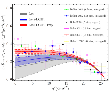
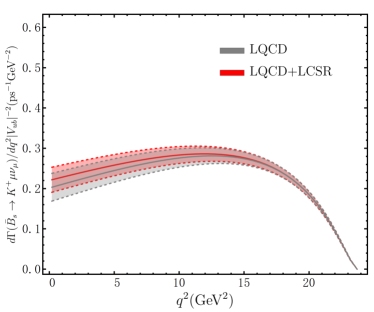
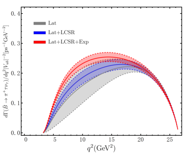
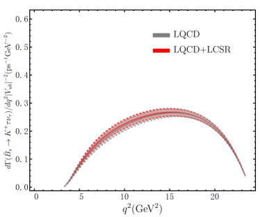
Figure 12: Theory predictions for the differential $q^{2}$ distributions of the exclusive semileptonic $B\to\pi\ell\bar{\nu}_{\ell}$ (left panel) and $B_{s}\to K\ell\bar{\nu}_{\ell}$ (right panel) decay processes in the entire kinematic region with the distinct BCL $z$-series fits of the form-factor shape parameters. The available experimental measurements on the binned $q^{2}$ distributions of the “golden” decay process $B\to\pi\mu\bar{\nu}_{\mu}$ from the BaBar [62, 63], Belle [64, 65] and Belle II [66] Collaborations are further displayed for an exploratory comparison.

We further display our final theory predictions for the differential $q^{2}$ distributions of the semileptonic $B_{(s)}\to\pi(K)\ell\bar{\nu}_{\ell}$ (with $\ell=\mu,\,\tau$) decay processes in the entire kinematic region in Figure 12, where the experimental measurements of the $B\to\pi\ell\bar{\nu}_{\ell}$ decay rates from the BaBar [62, 63], Belle [64, 65] and Belle II [66] Collaborations are further shown for a numerical comparison. In addition, we collect simultaneously the obtained numerical results from fitting the BCL $z$-series parameterizations with three distinct scenarios of the input data points: I) only synthetic lattice data points, II) synthetic lattice data points $\oplus$ LCSR results, III) synthetic lattice data points $\oplus$ LCSR results $\oplus$ experimental data. We can readily observe from Figure 12 that employing our improved LCSR predictions at large hadronic recoil in the BCL expansion fit program will be highly beneficial for pinning down the theory uncertainties from the particular fitting strategy with only the synthetic lattice data points. Moreover, we discover the slight tension of the predicted large-recoil $B\to\pi\mu\bar{\nu}_{\mu}$ decay distributions between the scenarios II) and III) fitting strategies with the BCL $z$-series parameterizations. With regard to the counterpart exclusive $B_{s}\to K\ell\bar{\nu}_{\ell}$ decay channels, taking into account the newly obtained LCSR data points in the numerical fit will bring about the moderate improvements on the resulting partial decay rates determined from fitting against only the synthetic lattice data points, as previously discussed in Section 4.2. For convenience, we also collect here our theory predictions for the total branching fractions of $B_{s}\to K\ell\bar{\nu}_{\ell}$ with the extracted interval of the CKM matrix element $|V_{ub}|$ shown in (136)

$$\mathcal{BR}(B_{s}\to K\mu\bar{\nu}_{\mu}) = (1.200\pm 0.128)\times 10^{-4}\,,$$

$$\mathcal{BR}(B_{s}\to K\tau\bar{\nu}_{\tau}) = (0.847\pm 0.078)\times 10^{-4}\,,$$ (138)

the former of which coincides well with the first experimental measurement from the LHCb Collaboration $\mathcal{BR}(B_{s}\to K\mu\bar{\nu}_{\mu})=\left[1.06\pm 0.05(\rm stat)\pm 0.08(\rm syst)\right]\times 10^{-4}$ [67] by employing the Cabibbo favored semileptonic $B_{s}\to D_{s}\ell\bar{\nu}_{\ell}$ decay process as the normalization channel. Unfortunately, both the two semitauonic bottom-meson decays $B\to\pi\tau\bar{\nu}_{\tau}$ and $B_{s}\to K\tau\bar{\nu}_{\tau}$ have not been observed in the high luminosity Belle II and LHCb experiments to date (see however the upper limit of ${\cal BR}(B\to\pi\tau\bar{\nu}_{\tau})<2.5\times 10^{-4}$ at the $90\,\%$ confidence level from the Belle Collaboration [162]).

Observables	Lattice QCD	Lattice QCD $\oplus$ LCSR	LCSR	This work
${\cal R}_{\pi}$	$0.69\pm 0.19$ [4]	$0.78\pm 0.10$ [164]	$0.69^{+0.03}_{-0.05}$ [25]	$0.720\pm 0.027\big{|}_{N=3}$
	$0.767\pm 0.145$ [163]	$0.699\pm 0.022$ [159]	$0.68^{+0.10}_{-0.09}$ [165]
	$0.838\pm 0.075$ [163]	$0.677\pm 0.010$ [161]	$0.65^{+0.13}_{-0.11}$ [165]	$0.746\pm 0.039\big{|}_{N=4}$
${\cal R}_{K}$	$0.77\pm 0.12$ [4]	$-$	$-$	$0.700\pm 0.016\big{|}_{N=3}$
	$0.695\pm 0.050$ [8]
	$0.836\pm 0.034$ [11]	$-$	$-$	$0.680\pm 0.019\big{|}_{N=4}$

Table 7: Theory predictions for the LFU ratios of the exclusive semileptonic $B_{(s)}\to\pi(K)\ell\bar{\nu}_{\ell}$ decay processes from the combined BCL expansion fitting against the synthetic lattice data points and the newly obtained LCSR results.

In light of the increasing sensitivity of the semitauonic bottom-hadron decays to the mysterious NP signature due to the very large $\tau$-lepton mass, we proceed to investigate two particular lepton-flavour-universality (LFU) probing observables for the exclusive $B_{(s)}\to\pi(K)\ell\bar{\nu}_{\ell}$ decays independent of the CKM matrix element $|V_{ub}|$

$${\cal R}_{\pi(K)}=\frac{\Gamma\left(B_{(s)}\to\pi(K)\tau\bar{\nu}_{\tau}\right)}{\Gamma\left(B_{(s)}\to\pi(K)\mu\bar{\nu}_{\nu}\right)}=\frac{\int_{m_{\tau}^{2}}^{q_{\rm max}^{2}}\,dq^{2}\,{d\Gamma(B_{(s)}\to\pi(K)\tau\bar{\nu}_{\tau})/dq^{2}}}{\int_{m_{\mu}^{2}}^{q_{\rm max}^{2}}\,dq^{2}\,{d\Gamma(B_{(s)}\to\pi(K)\mu\bar{\nu}_{\mu})/dq^{2}}}\,.$$ (139)

Apparently, precision predictions of such interesting LFU quantities would require a good knowledge of both the vector and scalar form factors in the whole semileptonic regions. Adopting the combined BCL $z$-series fit results with two distinct truncations $N\in\left\{3,\,4\right\}$ yields the desired numerical predictions for the two LFU observables as summarized in Table 7. Generally, our numerical results for ${\cal R}_{\pi(K)}$ are compatible with the previous theory determinations based upon the lattice simulation and LCSR methods. In addition, our BCL expansion fit result of the LFU ratio ${\cal R}_{\pi}$ can evidently accommodate the rather loose Belle measurement of ${\cal R}_{\pi}|_{\rm Belle\,\,2016}=1.05\pm 0.51$ [162]. We further present the resulting predictions for the two LFU ratios of the differential $B_{(s)}\to\pi(K)\ell\bar{\nu}_{\ell}$ decay distributions in Figure 13, which can be straightforwardly confronted with the counterpart numerical results from the RBC/UKQCD Collaborations [4], HPQCD [8] and FNAL/MILC [11] Collaborations.

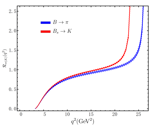
Figure 13: Theory predictions for the two interesting LFU ratios ${\cal R}_{\pi(K)}$ of the differential $B_{(s)}\to\pi(K)\ell\bar{\nu}_{\ell}$ decay distributions obtained from the combined BCL expansion fitting against the synthetic lattice data points and the newly obtained bottom-meson LCSR results.

Applying the two-fold differential spectrum of the flavour-changing charged-current $B_{q^{\prime}}\to M\ell\bar{\nu}_{\ell}$ decay process displayed in (130), we can construct two angular observables sensitive to Beyond the Standard Model (BSM) physics associated with electroweak symmetry breaking

$${\cal A}_{\rm FB}^{B_{(s)}\to\pi(K)\ell\bar{\nu}_{\ell}}(q^{2}) = \left[\frac{d\Gamma(B_{(s)}\to\pi(K)\ell\bar{\nu}_{\ell})}{dq^{2}}\right]^{-1}\,\int_{-1}^{1}d\cos\theta_{\ell}\,\,{\rm sgn}(\cos\theta_{\ell})\,\frac{d^{2}\Gamma(B_{(s)}\to\pi(K)\ell\bar{\nu}_{\ell})}{dq^{2}\,d\cos\theta_{\ell}}\,,$$ (140)

$$= \left[{1\over 2}\,b_{\theta_{\ell}}(q^{2})\right]:\left[a_{\theta_{\ell}}(q^{2})+{1\over 3}\,c_{\theta_{\ell}}(q^{2})\right]$$

$${\cal F}_{\rm H}^{B_{(s)}\to\pi(K)\ell\bar{\nu}_{\ell}}(q^{2}) = 1+{2\over 3}\,\left[\frac{d\Gamma(B_{(s)}\to\pi(K)\ell\bar{\nu}_{\ell})}{dq^{2}}\right]^{-1}\,{d^{2}\over d(\cos\theta_{\ell})^{2}}\,\frac{d^{2}\Gamma(B_{(s)}\to\pi(K)\ell\bar{\nu}_{\ell})}{dq^{2}\,d\cos\theta_{\ell}}$$ (141)

$$= \left[a_{\theta_{\ell}}(q^{2})+c_{\theta_{\ell}}(q^{2})\right]:\left[a_{\theta_{\ell}}(q^{2})+{1\over 3}\,c_{\theta_{\ell}}(q^{2})\right]\,.$$

Evidently, both the normalized forward-backward asymmetries ${\cal A}_{\rm FB}^{B_{(s)}\to\pi(K)\ell\bar{\nu}_{\ell}}$ and the $q^{2}$ differential flat terms ${\cal F}_{\rm H}^{B_{(s)}\to\pi(K)\ell\bar{\nu}_{\ell}}$ [157] will vanish in the massless lepton limit in the SM. Another appropriate candidate for the potential BSM probe can be introduced by investigating the polarization asymmetry of the final-state lepton

$${\cal A}_{\lambda_{\ell}}^{B_{(s)}\to\pi(K)\ell\bar{\nu}_{\ell}}(q^{2})=\left[\frac{d\Gamma(B_{(s)}\to\pi(K)\ell\bar{\nu}_{\ell})}{dq^{2}}\right]^{-1}\,\left[\frac{d\Gamma^{\lambda_{\ell}=-1/2}}{dq^{2}}-\frac{d\Gamma^{\lambda_{\ell}=+1/2}}{dq^{2}}\right]\left(B_{(s)}\to\pi(K)\ell\bar{\nu}_{\ell}\right)$$

$$=1-{2\over 3}\,\left\{\left[3\,\left(a_{\theta_{\ell}}(q^{2})+c_{\theta_{\ell}}(q^{2})\right)+{2\,m_{\ell}^{2}\over q^{2}-m_{\ell}^{2}}\,c_{\theta_{\ell}}(q^{2})\right]:\left[a_{\theta_{\ell}}(q^{2})+{1\over 3}\,c_{\theta_{\ell}}(q^{2})\right]\right\}\,,$$ (142)

which turns out to be sensitive to helicity-violating NP interactions. The analytic structure of the above-mentioned expression of the lepton polarization fraction (142) can be actually understood from the $\ell$-helicity conservation of the semileptonic $b\to q\ell\bar{\nu}_{\ell}$ transition in the massless lepton approximation in the SM. In order to facilitate the numerical comparisons with the future experimental measurements, we collect our theory predictions for the three different classes of the angular observables ${\cal A}_{\rm FB}^{B_{(s)}\to\pi(K)\ell\bar{\nu}_{\ell}}(q^{2})$, ${\cal F}_{\rm H}^{B_{(s)}\to\pi(K)\ell\bar{\nu}_{\ell}}(q^{2})$ and ${\cal A}_{\lambda_{\ell}}^{B_{(s)}\to\pi(K)\ell\bar{\nu}_{\ell}}(q^{2})$ in Figure 14. It is perhaps worthwhile to mention that our predictions for the normalized differential forward-backward asymmetries are in excellent agreement with the available lattice QCD simulation results from both the RBC/UKQCD [4] and HPQCD (without $B\to\pi\ell\bar{\nu}_{\ell}$) [8] Collaborations. On the other hand, the resulting predictions for the lepton polarization fractions of $B_{s}\to K\ell\bar{\nu}_{\ell}$ coincide well with the previous HPQCD [8] and FNAL/MILC [11] determinations (see also [166] for the numerical predictions with the vector and scalar $B_{s}\to K$ form factors computed with the TMD factorization approach). Moreover, we summarize our numerical predictions for the aforementioned three distinct classes of the integrated observables by employing the combined BCL expansion fit results of the semileptonic heavy-to-light $B_{(s)}\to\pi(K)$ form factors in Table 8, where we further confront our results with the previous determinations from the lattice QCD and LCSR techniques for convenience. Generally, our newly obtained results of the integrated angular observables for the semileptonic $B_{(s)}\to\pi(K)\ell\bar{\nu}_{\ell}$ decays are compatible with the available QCD determinations within the theory uncertainties, but with the exceptions of the previously extracted intervals of the flat terms ${\cal F}_{\rm H}^{B\to\pi\mu\bar{\nu}_{\mu}}$ and ${\cal F}_{\rm H}^{B\to\pi\tau\bar{\nu}_{\tau}}$ from [159], which turn out to be approximately one fourth of our numerical predictions individually. In order to better clarify such striking discrepancies, we can readily derive an exact but quite loose bound, independent of the scalar form-factor ratio, for the $q^{2}$ differential flat term by applying the explicit definition (141) as well as the kinematic constraint $q^{2}\in\left[m_{\ell}^{2}\,,(m_{B_{(s)}}-m_{\pi(K)})^{2}\right]$. For definiteness, we obtain

$${\cal F}_{\rm H}^{B_{(s)}\to\pi(K)\ell\bar{\nu}_{\ell}}(q^{2})\geq\frac{3}{1+2\,y_{\ell,\,{\rm max}}}\,,\qquad y_{\ell,\,{\rm max}}\equiv\left[\frac{m_{B_{(s)}}-m_{\pi(K)}}{m_{\ell}}\right]^{2}\,.$$ (143)

Plugging the input values for the emerged hadron and lepton masses summarized in Table 1 into (143) immediately leads to the desired numerical bounds

$${\cal F}_{\rm H}^{B\to\pi\mu\bar{\nu}_{\mu}}(q^{2})\geq 6.337\times 10^{-4}, {\cal F}_{\rm H}^{B\to\pi\tau\bar{\nu}_{\tau}}(q^{2})\geq 0.169\,,$$

$${\cal F}_{\rm H}^{B_{s}\to K\mu\bar{\nu}_{\mu}}(q^{2})\geq 7.049\times 10^{-4}, {\cal F}_{\rm H}^{B_{s}\to K\tau\bar{\nu}_{\tau}}(q^{2})\geq 0.187\,,$$ (144)

which are well respected by our combined BCL $z$-fit results for the corresponding four observables as collected in Table 8.

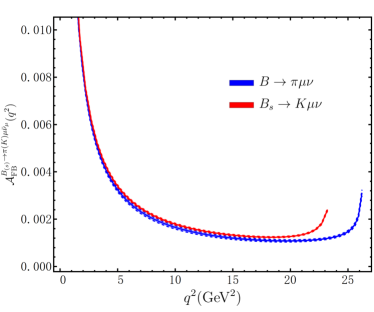
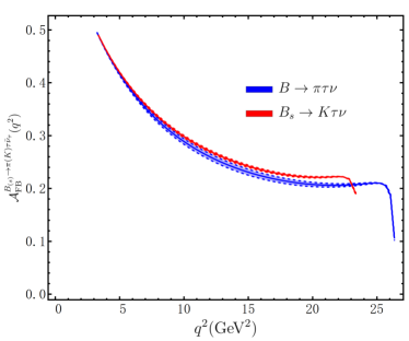
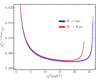
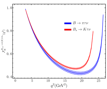
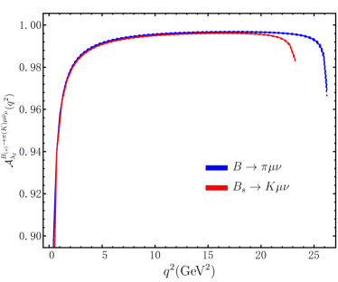
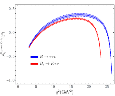
Figure 14: Theory predictions for the three distinct classes of the angular observables ${\cal A}_{\rm FB}^{B_{(s)}\to\pi(K)\ell\bar{\nu}_{\ell}}(q^{2})$, ${\cal F}_{\rm H}^{B_{(s)}\to\pi(K)\ell\bar{\nu}_{\ell}}(q^{2})$ and ${\cal A}_{\lambda_{\ell}}^{B_{(s)}\to\pi(K)\ell\bar{\nu}_{\ell}}(q^{2})$ obtained from the combined BCL expansion fitting against the synthetic lattice data points and the newly obtained bottom-meson LCSR results.

Observables	Lattice QCD	Lattice QCD $\oplus$ LCSR	This work
${\cal A}_{\rm FB}^{B\to\pi\mu\bar{\nu}_{\mu}}$			$\left(3.99\pm 0.35\right)\times 10^{-3}\big{|}_{N=3}$
	$\left(4.4\pm 1.3\right)\times 10^{-3}$ [4]	$\left(4.8\pm 0.3\right)\times 10^{-3}$ [159]
			$\left(3.72\pm 0.51\right)\times 10^{-3}\big{|}_{N=4}$
${\cal A}_{\rm FB}^{B\to\pi\tau\bar{\nu}_{\tau}}$			$0.248\pm 0.005\big{|}_{N=3}$
	$0.252\pm 0.012$ [4]	$0.259\pm 0.004$ [159]
			$0.244\pm 0.007\big{|}_{N=4}$
${\cal A}_{\rm FB}^{B_{s}\to K\mu\bar{\nu}_{\mu}}$	$\left(3.9\pm 1.1\right)\times 10^{-3}$ [4]		$\left(4.49\pm 0.21\right)\times 10^{-3}\big{|}_{N=3}$
	$\left(6.6\pm 1.0\right)\times 10^{-3}$ [8]	$-$
	$\left(3.21\pm 0.97\right)\times 10^{-3}$ [11]		$\left(5.14\pm 0.33\right)\times 10^{-3}\big{|}_{N=4}$
${\cal A}_{\rm FB}^{B_{s}\to K\tau\bar{\nu}_{\tau}}$	$0.2650\pm 0.0079$ [4]		$0.267\pm 0.002\big{|}_{N=3}$
	$0.284\pm 0.017$ [8]	$-$
	$0.2536\pm 0.0084$ [11]		$0.272\pm 0.003\big{|}_{N=4}$
${\cal F}_{\rm H}^{B\to\pi\mu\bar{\nu}_{\mu}}$			$\left(8.04\pm 0.72\right)\times 10^{-3}\big{|}_{N=3}$
	$-$	$\left(2.4\pm 0.1\right)\times 10^{-3}$ [159]
			$\left(7.52\pm 1.02\right)\times 10^{-3}\big{|}_{N=4}$
${\cal F}_{\rm H}^{B\to\pi\tau\bar{\nu}_{\tau}}$			$0.514\pm 0.012\big{|}_{N=3}$
	$-$	$0.134\pm 0.003$ [159]
			$0.508\pm 0.014\big{|}_{N=4}$
${\cal F}_{\rm H}^{B_{s}\to K\mu\bar{\nu}_{\mu}}$			$\left(9.10\pm 0.43\right)\times 10^{-3}\big{|}_{N=3}$
	$-$	$-$
			$\left(10.36\pm 0.67\right)\times 10^{-3}\big{|}_{N=4}$
${\cal F}_{\rm H}^{B_{s}\to K\tau\bar{\nu}_{\tau}}$			$0.555\pm 0.006\big{|}_{N=3}$
	$-$	$-$
			$0.565\pm 0.007\big{|}_{N=4}$
${\cal A}_{\lambda_{\ell}}^{B\to\pi\mu\bar{\nu}_{\mu}}$			$0.988\pm 0.001\big{|}_{N=3}$
	$-$	$-$
			$0.989\pm 0.002\big{|}_{N=4}$
${\cal A}_{\lambda_{\ell}}^{B\to\pi\tau\bar{\nu}_{\tau}}$			$0.266\pm 0.029\big{|}_{N=3}$
	$-$	$0.21\pm 0.02$ [159]
			$0.272\pm 0.032\big{|}_{N=4}$
${\cal A}_{\lambda_{\ell}}^{B_{s}\to K\mu\bar{\nu}_{\mu}}$			$0.987\pm 0.001\big{|}_{N=3}$
	$0.982^{+0.018}_{-0.079}$ [8]	$-$
			$0.985\pm 0.001\big{|}_{N=4}$
${\cal A}_{\lambda_{\ell}}^{B_{s}\to K\tau\bar{\nu}_{\tau}}$			$0.191\pm 0.014\big{|}_{N=3}$
	$0.105\pm 0.063$ [8]	$-$
			$0.172\pm 0.017\big{|}_{N=4}$

Table 8: Theory predictions for the three distinct classes of the integrated observables ${\cal A}_{\rm FB}^{B_{(s)}\to\pi(K)\ell\bar{\nu}_{\ell}}$, ${\cal F}_{\rm H}^{B_{(s)}\to\pi(K)\ell\bar{\nu}_{\ell}}$ and ${\cal A}_{\lambda_{\ell}}^{B_{(s)}\to\pi(K)\ell\bar{\nu}_{\ell}}$ obtained from the combined BCL $z$-series expansion fitting of the exclusive $B_{(s)}\to\pi(K)$ form factors against the synthetic lattice data points and the newly obtained bottom-meson LCSR results.

4.4 Phenomenological analysis of the $B\to K\nu_{\ell}\bar{\nu}_{\ell}$ observables

We are now in a position to explore phenomenological implications of the newly determined $B\to K$ form factors on the electroweak penguin $B\to K\nu_{\ell}\bar{\nu}_{\ell}$ decays, which are expected to be observed with first $10\,{\rm ab}^{-1}$ of the Belle II data [167] (see the earlier experimental searches by the BaBar [168], Belle [169] and Belle II [170] Collaborations). Importantly, the expected sensitivity of the total branching fraction for $B\to K\nu_{\ell}\bar{\nu}_{\ell}$ (summing over neutrino flavours) with $50\,{\rm ab}^{-1}$ of integrated luminosity has been estimated to be at the level of $10\,\%$, thus comparable to the current theoretical uncertainties of the SM predictions [68]. It is straightforward to derive the differential decay width formula for the theoretically cleanest FCNC $B^{0}\to K^{0}\nu_{\ell}\bar{\nu}_{\ell}$ decay process of the neutral bottom meson [171, 172]

$$\frac{d\Gamma(B^{0}\to K^{0}\nu_{\ell}\bar{\nu}_{\ell})}{dq^{2}} = {G_{F}^{2}\,\alpha_{\rm em}^{2}\over 256\,\pi^{5}}\,{\lambda^{3/2}(m_{B}^{2},m_{K}^{2},q^{2})\over m_{B}^{3}\,\sin^{4}\theta_{W}}\,|V_{tb}\,V_{ts}^{\ast}|^{2}\,\left[X_{t}\left({m_{t}^{2}\over m_{W}^{2}},{m_{H}^{2}\over m_{W}^{2}},\sin\theta_{W},\mu\right)\right]^{2}$$ (145)

$$\times\left|f_{BK}^{+}(q^{2})\right|^{2}\,,$$

where the CKM matrix elements $|V_{tb}|$ and $|V_{ts}^{\ast}|$ can be further evaluated from the four Wolfenstein parameters collected in Table 1 with the expanded matching relations at the accuracy of ${\cal O}(\lambda^{9})$ [173]. The short-distance Wilson coefficient $X_{t}$ can be expanded perturbatively in terms of the SM gauge couplings

$$X_{t}=X_{t}^{(0)}+{\alpha_{s}\over 4\pi}\,X_{t}^{{\rm QCD}(1)}+{\alpha_{\rm em}\over 4\pi}\,X_{t}^{{\rm EW}(1)}+...\,,$$ (146)

where the LO contribution $X_{t}^{(0)}$ [174], the NLO QCD correction $X_{t}^{{\rm QCD}(1)}$ [175, 176, 177] and the two-loop electroweak correction $X_{t}^{{\rm EW}(1)}$ [178] are already known analytically. By contrast, there exists an additional long-distance contribution to the counterpart charged channel $B^{-}\to K^{-}\nu_{\ell}\bar{\nu}_{\ell}$ due to the double charged-current interaction $B^{-}\to\tau(\to K^{-}\nu_{\tau})\,\bar{\nu}_{\tau}$ at tree level as originally discussed in [179]. In the narrow $\tau$-lepton width approximation ($\Gamma_{\tau}\simeq 2.3\times 10^{-3}\,{\rm eV}$ [89]), we can readily derive the tree-level charged-current contribution to the exclusive rare $B^{-}\to K^{-}\nu_{\tau}\bar{\nu}_{\tau}$ decay rate

$$\frac{d\Gamma(B^{-}\to K^{-}\nu_{\ell}\bar{\nu}_{\ell})}{dq^{2}}\bigg{|}_{\rm LD} = {G_{F}^{4}\,|V_{ub}V_{us}^{\ast}|^{2}\over 64\,\pi^{2}\,m_{B^{-}}^{3}}\,\left|f_{B^{-}}\,f_{K^{-}}\right|^{2}\,\frac{m_{\tau}^{3}}{\Gamma_{\tau}}\,\left[(m_{B^{-}}^{2}-m_{\tau}^{2})\,(m_{\tau}^{2}-m_{K^{-}}^{2})-m_{\tau}^{2}\,q^{2}\right],$$

where the invariant mass distribution of the two invisible particles satisfies the constraint [89]

$$0\leq q^{2}\leq\frac{(m_{B^{-}}^{2}-m_{\tau}^{2})\,(m_{\tau}^{2}-m_{K^{-}}^{2})}{m_{\tau}^{2}}\,.$$ (148)

At the first sight, this new mechanism will be suppressed by an extra factor of $G_{F}^{2}$ in comparison with the customary penguin contribution presented in (145). However, the very appearance of $1/\Gamma_{\tau}$ on the right-handed side of (LABEL:tree_contribution_to_B_to_K_nu_nu), due to the on-shell $\tau$-lepton enhancement, will be counted as ${\cal O}(G_{F}^{-2})$ parametrically, thus compensating the observed suppression factor [180]. Moreover, the interference effect between the tree and penguin amplitudes turns out to be numerically negligible (estimated to be at the order of $10^{-11}$ [179]) on account of the extremely small $\tau$-lepton width. We display in Figure 15 the yielding results for the differential decay distributions of $B^{0}\to K^{0}\nu_{\ell}\bar{\nu}_{\ell}$ and $B^{-}\to K^{-}\nu_{\ell}\bar{\nu}_{\ell}$ by employing the form factors determined from fitting the BCL $z$-series parameterizations with two distinct scenarios of the input data points: I) only synthetic lattice data points, II) synthetic lattice data points $\oplus$ LCSR results.

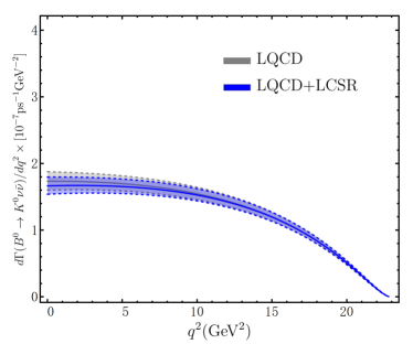
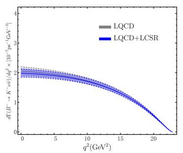
Figure 15: Theory predictions for the differential decay distributions of $B^{0}\to K^{0}\nu_{\ell}\bar{\nu}_{\ell}$ (left panel) and $B^{-}\to K^{-}\nu_{\ell}\bar{\nu}_{\ell}$ (right panel) by applying the form factors determined from the two distinct scenarios of the BCL $z$-series expansion fitting strategies.

In order to confront our numerical predictions with the anticipated measurements from the high-luminosity Belle II experiment, we introduce the following three $q^{2}$-binned observables for the semileptonic $B\to K\nu_{\ell}\bar{\nu}_{\ell}$ decays [35]

$$\Delta{\cal BR}^{B^{0}\to K^{0}\nu_{\ell}\bar{\nu}_{\ell}}(q_{1}^{2},\,q_{2}^{2})=\tau_{B^{0}}\,\int_{q_{1}^{2}}^{q_{2}^{2}}\,dq^{2}\,\frac{d\Gamma(B^{0}\to K^{0}\nu_{\ell}\bar{\nu}_{\ell})}{dq^{2}}\,,$$

$$\Delta{\cal BR}^{B^{-}\to K^{-}\nu_{\ell}\bar{\nu}_{\ell}}(q_{1}^{2},\,q_{2}^{2})=\tau_{B^{-}}\,\int_{q_{1}^{2}}^{q_{2}^{2}}\,dq^{2}\,\frac{d\Gamma(B^{-}\to K^{-}\nu_{\ell}\bar{\nu}_{\ell})}{dq^{2}}\,,$$

$${\cal R}_{K\pi}(q_{1}^{2},\,q_{2}^{2})=\left[\int_{q_{1}^{2}}^{q_{2}^{2}}\,dq^{2}\,\frac{d\Gamma(B^{0}\to K^{0}\nu_{\ell}\bar{\nu}_{\ell})}{dq^{2}}\right]:\left[\int_{q_{1}^{2}}^{q_{2}^{2}}\,dq^{2}\,\frac{d\Gamma(B^{0}\to\pi^{-}\bar{\nu}_{\mu}\nu_{\mu})}{dq^{2}}\right]\,,$$ (149)

where the ratio of partially integrated differential branching fractions ${\cal R}_{K\pi}$ is expected to suffer from the lower hadronic uncertainties due to the correlations between the exclusive $B\to\pi$ and $B\to K$ form factors. We summarize our final predictions for these three quantities with the choice of the $q^{2}$ intervals following [68] in Table 9, where we further display the previous theoretical determinations with the lattice simulation and LCSR methods for convenience.

$[q_{1}^{2},\,q_{2}^{2}]$    (${\rm in\,\,GeV}^{2}$)	$10^{6}\times\Delta{\cal BR}^{B^{0}\to K^{0}\nu_{\ell}\bar{\nu}_{\ell}}(q_{1}^{2},q_{2}^{2})$	$10^{6}\times\Delta{\cal BR}^{B^{-}\to K^{-}\nu_{\ell}\bar{\nu}_{\ell}}(q_{1}^{2},q_{2}^{2})$	$10^{2}\times{\cal R}_{K\pi}(q_{1}^{2},q_{2}^{2})$
$[0.0,1.0]$	$0.253^{+0.020}_{-0.019}$	$0.324^{+0.023}_{-0.021}$	$3.949\pm 0.319$
$[1.0,2.5]$	$0.381^{+0.028}_{-0.027}$	$0.482^{+0.033}_{-0.030}$	$3.932\pm 0.303$
$[2.5,4.0]$	$0.380^{+0.027}_{-0.025}$	$0.476^{+0.031}_{-0.029}$	$3.904\pm 0.289$
$[4.0,6.0]$	$0.502^{+0.034}_{-0.032}$	$0.622^{+0.039}_{-0.035}$	$3.859\pm 0.278$
$[6.0,8.0]$	$0.492^{+0.032}_{-0.030}$	$0.602^{+0.037}_{-0.034}$	$3.788\pm 0.270$
$[8.0,12.0]$	$0.924^{+0.058}_{-0.053}$	$1.112^{+0.066}_{-0.060}$	$3.626\pm 0.262$
$[12.0,16.0]$	$0.776^{+0.047}_{-0.043}$	$0.916^{+0.053}_{-0.048}$	$3.245\pm 0.238$
$\left[16.0,\,(m_{B}-m_{K})^{2}\right]$	$0.607^{+0.036}_{-0.032}$	$0.705^{+0.040}_{-0.036}$	$1.918\pm 0.129$
$\left[0.0,\,(m_{B}-m_{K})^{2}\right]$	$6.02^{+1.68}_{-1.76}$ [35]	$5.10\pm 0.80$ [171]	$-$
	$4.01\pm 0.49$ [180]	$3.98\pm 0.47$ [172]	$-$
	$4.67\pm 0.35$ [181]	$4.94\pm 0.52$ [180]	$-$
	$4.1^{+1.3}_{-1.0}$ [182]	$5.67\pm 0.38$ [181]	$-$
	$4.4\pm 1.5$ [183]	$4.53\pm 0.64$ [184]	$-$
	$-$	$4.65\pm 0.62$ [185]	$-$
	$4.315^{+0.271}_{-0.248}$ (this work)	$5.239^{+0.311}_{-0.281}$ (this work)	$3.240\pm 0.211$ (this work)

Table 9: Theory predictions for the three partially integrated differential observables $\Delta{\cal BR}^{B^{0}\to K^{0}\nu_{\ell}\bar{\nu}_{\ell}}$, $\Delta{\cal BR}^{B^{-}\to K^{-}\nu_{\ell}\bar{\nu}_{\ell}}$, and ${\cal R}_{K\pi}$ (see (149) for their explicit definitions) obtained from the combined BCL $z$-series expansion fitting of the exclusive $B\to\pi,K$ form factors against the synthetic lattice data points and the newly obtained bottom-meson LCSR results.

5 Conclusions

In the current paper we have carried out the improved computations of the semileptonic $B_{d,s}\to\pi,K$ decay form factors at large hadronic recoil, which evidently belong to the most important hadronic quantities in heavy quark physics, by employing the method of light-cone sum rules (LCSR) in soft-collinear effective theory (SCET) with both the leading-twist and higher-twist bottom-meson distribution amplitudes. In particular, we have computed for the first time the non-vanishing spectator-quark mass corrections to these form factors at NLO in the strong coupling constant, which appeared to preserve the approximated large-recoil symmetry relations for the heavy-to-light transition form factors and turned out to escape from an extra suppression of the powers of $\Lambda_{\rm QCD}/m_{b}$ in heavy quark expansion. Our explicit sum rules for these spectator-quark mass corrections further implied that evaluating such SU(3)-flavour symmetry breaking effects directly with the perturbative factorization technique would result in the soft-collinear convolution integrals with the notorious rapidity singularities. Moreover, we have accomplished the complete NLL resummation for the parametrically enhanced logarithms of $m_{b}/\Lambda_{\rm QCD}$ entering in the factorized expressions of the leading-power contributions to the considered vacuum-to-bottom-meson correlation functions displayed in (2) by taking advantage of the standard renormalization-group formalism in momentum space. We then proceeded to explore the four distinct classes of the NLP contributions to the exclusive $B_{d,s}\to\pi,K$ form factors with the same LCSR technique at tree level: I) the higher-order terms from heavy quark expansion of the hard-collinear quark propagator, II) the subleading power corrections from the effective matrix element of the ${\rm SCET_{I}}$ weak current $(\bar{\xi}_{\rm hc}\,W_{\rm hc})\,\gamma_{\mu}\,\left[i\,{\not{D}}_{\top}/\left(2\,m_{b}\right)\right]\,h_{v}$, III) the higher-twist corrections from the two-particle and three-particle heavy quark effective theory (HQET) distribution amplitudes, IV) the four-particle twist-five and twist-six contributions in the factorization approximation. We have extensively used the nontrivial operator identities between the two-body and three-body light-cone HQET operators due to the classical equations of motion in our constructions of the NLP sum rules. Interestingly, we observed that only the particular class-I NLP contribution from the expanded hard-collinear propagator can generate the large-recoil symmetry violation effect between the vector and scalar form factors, while both the class-I and class-II NLP corrections can yield the symmetry breaking effects between the vector and tensor form factors at large hadronic recoil.

Having at our disposal the updated SCET sum rules for the exclusive heavy-to-light bottom-meson decay form factors, we turned to investigate the numerical implications of the NLL resummation improved leading-power contributions and the newly obtained four classes of the NLP corrections at tree level on the theory predictions for the semileptonic $B_{d,s}\to\pi,K$ form factors of our interest, by employing the general three-parameter ansatz for the necessary HQET distribution amplitudes. It has been explicitly shown that the most prominent subleading power contribution arises from the two-particle twist-five off-light-cone correction, which can reduce the corresponding leading-power LCSR predictions in the kinematic region $0\leq q^{2}\leq 8\,{\rm GeV^{2}}$ by an amount of $(25-30)\,\%$ numerically. On the contrary, the yielding impacts from the four-particle higher-twist bottom-meson distribution amplitudes have been demonstrated to be numerically insignificant in the factorization approximation owing to the smallness of the normalization constant $|\langle\bar{q}q\rangle:(\lambda_{B}\,s_{0})|\simeq 10\,\%$ in the tree-level sum rules (75). In addition, the higher-order QCD corrections to the short-distance matching coefficients appeared in the leading-power SCET sum rules can bring about consistently ${\cal O}(30\,\%)$ reductions of the counterpart leading-order LCSR predictions. It remains important to remark that our numerical results for the semileptonic bottom-meson decay form factors indicate the following hierarchy relations $f_{BK}^{+\,(T)}(0)>f_{B_{s}K}^{+\,(T)}(0)>f_{B\pi}^{+\,(T)}(0)$ in the maximal recoil limit. Remarkably, we predicted very sizeable SU(3)-flavour symmetry violating effects between the exclusive $B\to\pi$ and $B\to K$ form factors based upon the established LCSR with the HQET distribution amplitudes: numerically ${\cal O}(30\,\%)$ for the two form-factor ratios ${\cal R}_{\rm SU(3)}^{+,\,0}$ and ${\cal O}(40\,\%)$ for the particular ratio ${\cal R}_{\rm SU(3)}^{T}$.

Subsequently, we extrapolated the bottom-meson LCSR computations for the exclusive $B_{d,s}\to\pi,K$ form factors towards the large momentum transfer $q^{2}$ with the aid of the Bourrely-Caprini-Lellouch (BCL) $z$-series parameterizations for these form factors. It is interesting to note that including the newly obtained LCSR predictions at small momentum transfer in our numerical fitting procedure turned out to be highly beneficial for pinning down the theory uncertainties of all the three $B\to\pi$ form factors in the kinematic regime $0.10\leq z(q^{2})\leq 0.31$ significantly, due to the yet non-negligible errors of the lattice QCD results from the RBC/UKQCD Collaboration [4] (numerically at the level of $(8.4-14.3)\,\%$ for the vector form factor and $(7.6-13.6)\,\%$ for the scalar form factor). Furthermore, we have confronted our combined BCL fit results of the $B\to\pi$ form factors with the theoretical expectations from the particular low-recoil symmetry relations (119) and (124), on account of the combination of the heavy quark spin symmetry and the so-called soft-pion approximation, in Figures (8) and (9) manifestly. Additionally, the available high-precision lattice QCD results of the semileptonic $B\to K$ form factors from both the FNAL/MILC Collaboration [14] and the HPQCD Collaboration [15] appeared to be in tension with the strongly correlated predictions from the improved bottom-meson LCSR determinations, when carrying out the numerical interpolations between the lattice simulation and LCSR results with the standard BCL $z$-series expansions. With regard to the flavour-changing charged-current $B_{s}\to K\ell\bar{\nu}_{\ell}$ form factors, the yielding BCL fit results for the three coefficients $b_{0,1,2}^{T}$ in Table 4 became more uncertain in comparison with the counterpart results for the $z$-expansion parameters of the tensor $B\to\pi$ form factor, due to the very absence of the lattice data points for $f_{B_{s}K}^{T}(q^{2})$ in the lower recoil region. Importantly, we indeed benefited from the combined BCL $z$-expansion fit to both the LCSR and lattice simulation results by improving further the theory accuracy of the vector and scalar form factors $f_{B_{s}K}^{+,\,0}(q^{2})$, numerically at the level of ${\cal O}(20\,\%)$, when compared with the counterpart BCL fitting procedure with the “only lattice QCD” data points. It has been verified that our BCL $z$-fit predictions for the scalar form-factor ratios of both the exclusive $B\to K$ and $B_{s}\to K$ form factors at the zero-recoil limit differ from the expected Isgur-Wise relations due to the combined heavy quark and chiral symmetries enormously, thus supporting the previous lattice simulation results from the FNAL/MILC Collaboration [14].

Performing the simultaneous BCL expansion fit to the SCET sum rules, lattice QCD and experimental data points enabled us to extract the desired CKM matrix element $|V_{ub}|$ from the “golden” exclusive process $B\to\pi\ell\bar{\nu}_{\ell}$ with the two distinct truncations

$$\left|V_{ub}\right|_{B\to\pi\ell\bar{\nu}_{\ell}}=(3.76\pm 0.13)\times\,10^{-3}\,,\qquad({\rm BCL\,\,fit\,\,with}\,\,N=3)$$

$$\left|V_{ub}\right|_{B\to\pi\ell\bar{\nu}_{\ell}}=(3.72\pm 0.14)\times\,10^{-3}\,.\qquad({\rm BCL\,\,fit\,\,with}\,\,N=4)$$ (150)

We are therefore led to conclude that truncating the $z$-series expansions at the order $N=3$ in the numerical fit procedure can indeed be justified for the practical purpose due to the apparent stability against the truncation order. Our numerical predictions for the two particular lepton-flavour-universality (LFU) ratios for the exclusive $B_{(s)}\to\pi(K)\ell\bar{\nu}_{\ell}$ decays have been collected in Figure 13 and Table 7, and we quote here the obtained results for such gold-plated quantities

$${\cal R}_{\pi}=0.720\pm 0.027\,,\qquad{\cal R}_{K}=0.700\pm 0.016\,,\qquad({\rm BCL\,\,fit\,\,with}\,\,N=3)$$

$${\cal R}_{\pi}=0.746\pm 0.039\,,\qquad{\cal R}_{K}=0.680\pm 0.019\,.\qquad({\rm BCL\,\,fit\,\,with}\,\,N=4)$$ (151)

The yielding results for the three different classes of the angular observables sensitive to the potential Beyond the Standard Model (BSM) physics ${\cal A}_{\rm FB}^{B_{(s)}\to\pi(K)\ell\bar{\nu}_{\ell}}$, ${\cal F}_{\rm H}^{B_{(s)}\to\pi(K)\ell\bar{\nu}_{\ell}}$ and ${\cal A}_{\lambda_{\ell}}^{B_{(s)}\to\pi(K)\ell\bar{\nu}_{\ell}}$ have been explicitly displayed in Figure 14 and Table 8, where the previous theory determinations from the lattice simulation and LCSR approaches were further shown for a comparison. We finally presented our numerical predictions for the three partially integrated differential observables $\Delta{\cal BR}^{B^{0}\to K^{0}\nu_{\ell}\bar{\nu}_{\ell}}$, $\Delta{\cal BR}^{B^{-}\to K^{-}\nu_{\ell}\bar{\nu}_{\ell}}$, and ${\cal R}_{K\pi}$ (see (149) for their explicit definitions) for the exclusive rare $B\to K\nu_{\ell}\bar{\nu}_{\ell}$ decays in Table 9.

Future developments of the theory predictions for the heavy-to-light bottom-meson decays beyond our work can be pursued forward in a variety of directions. First, it would be interesting to perform the full two-loop QCD computations of the semileptonic $B_{d,s}\to\pi,K$ decay form factors at large hadronic recoil, by employing the SCET sum rules framework, in order to reduce further the current perturbative uncertainties displayed in Figures 3 and 4. Actually, the desired hard matching coefficients in the ${\rm SCET_{I}}$ representations of the flavour-changing QCD currents $\bar{q}\,\Gamma_{i}\,b$ have been already determined at the ${\cal O}(\alpha_{s}^{2})$ accuracy. The only missing ingredients for constructing the two-loop factorization formulae of the very vacuum-to-bottom-meson correlation functions (2) consist in the yet unknown short-distance Wilson coefficients in the second-step ${\rm SCET_{I}}\to{\rm SCET_{II}}$ matching procedure. Second, investigating the subleading-power contributions to the exclusive $B_{d,s}\to\pi,K$ form factors systematically with the effective field theory techniques and then evaluating the resulting (non)-local soft-collinear matrix elements with the appropriate nonperturbative QCD methods will be evidently in high demand from both the conceptual and phenomenological perspectives. As a matter of fact, it would be of utmost importance to achieve the analytical regularization of the unwanted end-point divergences entering in the factorized expressions of the ${\rm SCET_{I}}$ matrix elements for the two-body $A$-type currents. Third, advancing our knowledge of the poorly constrained bottom-meson distribution amplitudes in HQET with model-independent techniques (for instance, along the line of [128]) will be indispensable for enhancing further our predictive power of the exclusive bottom-meson decay matrix elements in the theory frameworks of both QCD factorization and light-cone sum rules. In particular the yielding noticeable uncertainties due to the two-particle $B_{d,s}$-meson distribution amplitudes has already become the major stumbling block for accomplishing precision calculations of a wide range of the interesting physical observables accessible at the LHCb and Belle II experiments. Fourth, the established strategies of evaluating the subleading-power $B_{d,s}\to\pi,K$ matrix elements can be further extended to compute the NLP corrections to the analogous heavy-to-light $B\to\rho,\omega,K^{\ast}$ decay form factors (thus going well beyond our previous work [37]) and to explore the delicate strong interaction mechanisms dictating the Cabibbo favored semileptonic $B_{(s)}\to D_{(s)}^{\ast}\ell\bar{\nu}_{\ell}$ decay processes.

References

• [1] Y.Β Amhis et al. [HFLAV], β€œAverages of $b$-hadron, $c$-hadron, and $\tau$-lepton properties as of 2021,” [arXiv:2206.07501 [hep-ex]].
• [2] E.Β Dalgic, A.Β Gray, M.Β Wingate, C.Β T.Β H.Β Davies, G.Β P.Β Lepage and J.Β Shigemitsu, β€œB meson semileptonic form-factors from unquenched lattice QCD,” Phys. Rev. D 73 (2006), 074502; [Erratum: Phys. Rev. D 75 (2007), 119906] [arXiv:hep-lat/0601021 [hep-lat]].
• [3] J.Β A.Β Bailey et al. [Fermilab Lattice and MILC], $|V_{ub}|$ from $B\to\pi\ell\nu$ decays and (2+1)-flavor lattice QCD,” Phys. Rev. D 92 (2015) 014024 [arXiv:1503.07839 [hep-lat]].
• [4] J.Β M.Β Flynn, T.Β Izubuchi, T.Β Kawanai, C.Β Lehner, A.Β Soni, R.Β S.Β Van de Water and O.Β Witzel, β€œ Bβ†’Ο€β€‹β„“β€‹Ξ½β†’π΅πœ‹β„“πœˆB\to\pi\ell\nu and Bsβ†’K​ℓ​ν→subscriptπ΅π‘ πΎβ„“πœˆB_{s}\to K\ell\nu form factors and $|V_{ub}|$ from 2+1-flavor lattice QCD with domain-wall light quarks and relativistic heavy quarks,” Phys. Rev. D 91 (2015) 074510 [arXiv:1501.05373 [hep-lat]].
• [5] B.Β Colquhoun, R.Β J.Β Dowdall, J.Β Koponen, C.Β T.Β H.Β Davies and G.Β P.Β Lepage, $B\to\pi\ell\nu$ at zero recoil from lattice QCD with physical $u/d$ quarks,” Phys. Rev. D 93 (2016) 034502 [arXiv:1510.07446 [hep-lat]].
• [6] B.Β Colquhoun et al. [JLQCD], β€œForm factors of $B\to\pi\ell\nu$ and a determination of $|V_{ub}|$ with MΓΆbius domain-wall fermions,” Phys. Rev. D 106 (2022) 054502 doi:10.1103/PhysRevD.106.054502 [arXiv:2203.04938 [hep-lat]].
• [7] J.Β A.Β Bailey et al. [Fermilab Lattice and MILC], $B\to\pi\ell\ell$ form factors for new-physics searches from lattice QCD,” Phys. Rev. Lett. 115 (2015) 152002 [arXiv:1507.01618 [hep-ph]].
• [8] C.Β M.Β Bouchard, G.Β P.Β Lepage, C.Β Monahan, H.Β Na and J.Β Shigemitsu, β€œBsβ†’K​ℓ​ν→subscriptπ΅π‘ πΎβ„“πœˆB_{s}\to K\ell\nu form factors from lattice QCD,” Phys. Rev. D 90 (2014) 054506 [arXiv:1406.2279 [hep-lat]].
• [9] F.Β Bahr et al. [ALPHA], β€œContinuum limit of the leading-order HQET form factor in Bsβ†’K​ℓ​ν→subscriptπ΅π‘ πΎβ„“πœˆB_{s}\to K\ell\nu decays,” Phys. Lett. B 757 (2016) 473 [arXiv:1601.04277 [hep-lat]].
• [10] C.Β J.Β Monahan, C.Β M.Β Bouchard, G.Β P.Β Lepage, H.Β Na and J.Β Shigemitsu, β€œForm factor ratios for Bsβ†’K​ℓ​ν→subscriptπ΅π‘ πΎβ„“πœˆB_{s}\rightarrow K\,\ell\,\nu and Bsβ†’Ds​ℓ​ν→subscript𝐡𝑠subscriptπ·π‘ β„“πœˆB_{s}\rightarrow D_{s}\,\ell\,\nu semileptonic decays and $|V_{ub}/V_{cb}|$,” Phys. Rev. D 98 (2018) 114509 [arXiv:1808.09285 [hep-lat]].
• [11] A.Β Bazavov et al. [Fermilab Lattice and MILC], β€œBsβ†’K​ℓ​ν→subscriptπ΅π‘ πΎβ„“πœˆB_{s}\to K\ell\nu decay from lattice QCD,” Phys. Rev. D 100 (2019) 034501 [arXiv:1901.02561 [hep-lat]].
• [12] F.Β Bahr, D.Β Banerjee, F.Β Bernardoni, M.Β Koren, H.Β Simma and R.Β Sommer, β€œExtraction of bare form factors for Bsβ†’K​ℓ​ν→subscriptπ΅π‘ πΎβ„“πœˆB_{s}\to K\ell\nu decays in nonperturbative HQET,” Int. J. Mod. Phys. A 34 (2019) 1950166 [arXiv:1903.05870 [hep-lat]].
• [13] C.Β Bouchard et al. [HPQCD], β€œRare decay $B\to K\ell^{+}\ell^{-}$ form factors from lattice QCD,” Phys. Rev. D 88 (2013) 054509; [Erratum: Phys. Rev. D 88 (2013) 079901] [arXiv:1306.2384 [hep-lat]].
• [14] J.Β A.Β Bailey, A.Β Bazavov, C.Β Bernard, C.Β M.Β Bouchard, C.Β DeTar, D.Β Du, A.Β X.Β El-Khadra, J.Β Foley, E.Β D.Β Freeland and E.Β GΓ‘miz, et al. $B\to Kl^{+}l^{-}$ Decay Form Factors from Three-Flavor Lattice QCD,” Phys. Rev. D 93 (2016) 025026 [arXiv:1509.06235 [hep-lat]].
• [15] W.Β G.Β Parrott et al. [HPQCD], $B\to K$ and $D\to K$ form factors from fully relativistic lattice QCD,” [arXiv:2207.12468 [hep-lat]].
• [16] Y.Β Aoki et al. [Flavour Lattice Averaging Group (FLAG)], β€œFLAG Review 2021,” Eur. Phys. J. C 82 (2022) 869 [arXiv:2111.09849 [hep-lat]].
• [17] P.Β A.Β Boyle, B.Β Chakraborty, C.Β T.Β H.Β Davies, T.Β DeGrand, C.Β DeTar, L.Β Del Debbio, A.Β X.Β El-Khadra, F.Β Erben, J.Β M.Β Flynn and E.Β GΓ‘miz, et al. β€œA lattice QCD perspective on weak decays of $b$ and $c$ quarks Snowmass 2022 White Paper,” [arXiv:2205.15373 [hep-lat]].
• [18] A.Β Di Canto and S.Β Meinel, β€œWeak Decays of $b$ and $c$ Quarks,” [arXiv:2208.05403 [hep-ex]].
• [19] V.Β M.Β Belyaev, A.Β Khodjamirian and R.Β Ruckl, β€œQCD calculation of the $B\to\pi,K$ form-factors,” Z. Phys. C 60 (1993) 349 [arXiv:hep-ph/9305348 [hep-ph]].
• [20] A.Β V.Β Rusov, β€œHigher-twist effects in light-cone sum rule for the $B\rightarrow\pi$ form factor,” Eur. Phys. J. C 77 (2017) 442 [arXiv:1705.01929 [hep-ph]].
• [21] A.Β Khodjamirian, R.Β Ruckl, S.Β Weinzierl and O.Β I.Β Yakovlev, β€œPerturbative QCD correction to the $B\rightarrow\pi$ transition form-factor,” Phys. Lett. B 410 (1997) 275 [arXiv:hep-ph/9706303 [hep-ph]].
• [22] E.Β Bagan, P.Β Ball and V.Β M.Β Braun, β€œRadiative corrections to the decay $B\rightarrow\pi e\nu$ and the heavy quark limit,” Phys. Lett. B 417 (1998) 154 [arXiv:hep-ph/9709243 [hep-ph]].
• [23] P.Β Ball and R.Β Zwicky, β€œNew results on $B\to\pi,K,\eta$ decay formfactors from light-cone sum rules,” Phys. Rev. D 71 (2005) 014015 [arXiv:hep-ph/0406232 [hep-ph]].
• [24] G.Β Duplancic, A.Β Khodjamirian, T.Β Mannel, B.Β Melic and N.Β Offen, β€œLight-cone sum rules for $B\to\pi$ form factors revisited,” JHEP 04 (2008) 014 [arXiv:0801.1796 [hep-ph]].
• [25] A.Β Khodjamirian, T.Β Mannel, N.Β Offen and Y.Β M.Β Wang, $B\to\pi\ell\nu_{l}$ Width and $|V_{ub}|$ from QCD Light-Cone Sum Rules,” Phys. Rev. D 83 (2011) 094031 [arXiv:1103.2655 [hep-ph]].
• [26] A.Β Bharucha, β€œTwo-loop Corrections to the $B\to\pi$ Form Factor from QCD Sum Rules on the Light-Cone and $|V_{ub}|$,” JHEP 05 (2012) 092 [arXiv:1203.1359 [hep-ph]].
• [27] V.Β M.Β Braun, G.Β P.Β Korchemsky and D.Β MΓΌller, β€œThe Uses of conformal symmetry in QCD,” Prog. Part. Nucl. Phys. 51 (2003) 311 [arXiv:hep-ph/0306057 [hep-ph]].
• [28] P.Β Colangelo and A.Β Khodjamirian, β€œQCD sum rules, a modern perspective,” [arXiv:hep-ph/0010175 [hep-ph]].
• [29] A.Β Khodjamirian, T.Β Mannel and N.Β Offen, β€œB𝐡B-meson distribution amplitude from the $B\to\pi$ form-factor,” Phys. Lett. B 620 (2005) 52 [arXiv:hep-ph/0504091 [hep-ph]].
• [30] A.Β Khodjamirian, T.Β Mannel and N.Β Offen, β€œForm-factors from light-cone sum rules with $B$-meson distribution amplitudes,” Phys. Rev. D 75 (2007) 054013 [arXiv:hep-ph/0611193 [hep-ph]].
• [31] F.Β De Fazio, T.Β Feldmann and T.Β Hurth, β€œLight-cone sum rules in soft-collinear effective theory,” Nucl. Phys. B 733 (2006) 1; [Erratum: Nucl. Phys. B 800 (2008), 405] [arXiv:hep-ph/0504088 [hep-ph]].
• [32] F.Β De Fazio, T.Β Feldmann and T.Β Hurth, β€œSCET sum rules for $B\to P$ and $B\to V$ transition form factors,” JHEP 02 (2008) 031 [arXiv:0711.3999 [hep-ph]].
• [33] Y.Β M.Β Wang and Y.Β L.Β Shen, β€œQCD corrections to $B\to\pi$ form factors from light-cone sum rules,” Nucl. Phys. B 898 (2015), 563-604 [arXiv:1506.00667 [hep-ph]].
• [34] Y.Β L.Β Shen, Y.Β B.Β Wei and C.Β D.Β LΓΌ, β€œRenormalization group analysis of $B\to\pi$ form factors with $B$-meson light-cone sum rules,” Phys. Rev. D 97 (2018) no.5, 054004 [arXiv:1607.08727 [hep-ph]].
• [35] C.Β D.Β LΓΌ, Y.Β L.Β Shen, Y.Β M.Β Wang and Y.Β B.Β Wei, β€œQCD calculations of $B\to\pi,K$ form factors with higher-twist corrections,” JHEP 01 (2019), 024 [arXiv:1810.00819 [hep-ph]].
• [36] N.Β Gubernari, A.Β Kokulu and D.Β van Dyk, $B\to P$ and $B\to V$ Form Factors from $B$-Meson Light-Cone Sum Rules beyond Leading Twist,” JHEP 01 (2019) 150 [arXiv:1811.00983 [hep-ph]].
• [37] J.Β Gao, C.Β D.Β LΓΌ, Y.Β L.Β Shen, Y.Β M.Β Wang and Y.Β B.Β Wei, β€œPrecision calculations of $B\to V$ form factors from soft-collinear effective theory sum rules on the light-cone,” Phys. Rev. D 101 (2020) 074035 [arXiv:1907.11092 [hep-ph]].
• [38] Y.Β L.Β Shen and Y.Β B.Β Wei, $B\to P,V$ Form Factors with the B-Meson Light-Cone Sum Rules,” Adv. High Energy Phys. 2022 (2022) 2755821 [arXiv:2112.01500 [hep-ph]].
• [39] Y.Β M.Β Wang, Y.Β B.Β Wei, Y.Β L.Β Shen and C.Β D.Β LΓΌ, β€œPerturbative corrections to $B\to D$ form factors in QCD,” JHEP 06 (2017), 062 [arXiv:1701.06810 [hep-ph]].
• [40] J.Β Gao, T.Β Huber, Y.Β Ji, C.Β Wang, Y.Β M.Β Wang and Y.Β B.Β Wei, $B\to D$ form factors beyond leading power and extraction of $|V_{cb}|$ and $R(D)$,” JHEP 05 (2022) 024 [arXiv:2112.12674 [hep-ph]].
• [41] Y.Β M.Β Wang, Y.Β L.Β Shen and C.Β D.Β LΓΌ, $\Lambda_{b}\to p,\Lambda$ transition form factors from QCD light-cone sum rules,” Phys. Rev. D 80 (2009) 074012 [arXiv:0907.4008 [hep-ph]].
• [42] T.Β Feldmann and M.Β W.Β Y.Β Yip, β€œForm factors for $\Lambda_{b}\to\Lambda$ transitions in the soft-collinear effective theory,” Phys. Rev. D 85 (2012), 014035; [Erratum: Phys. Rev. D 86 (2012), 079901] [arXiv:1111.1844 [hep-ph]].
• [43] Y.Β M.Β Wang and Y.Β L.Β Shen, β€œPerturbative Corrections to $\Lambda_{b}\to\Lambda$ Form Factors from QCD Light-Cone Sum Rules,” JHEP 02 (2016), 179 [arXiv:1511.09036 [hep-ph]].
• [44] Y.Β Y.Β Keum, H.Β N.Β Li and A.Β I.Β Sanda, β€œPenguin enhancement and $B\to K\pi$ decays in perturbative QCD,” Phys. Rev. D 63 (2001), 054008 [arXiv:hep-ph/0004173 [hep-ph]].
• [45] C.Β D.Β LΓΌ, K.Β Ukai and M.Β Z.Β Yang, β€œBranching ratio and CP violation of $B\to\pi\pi$ decays in perturbative QCD approach,” Phys. Rev. D 63 (2001), 074009 [arXiv:hep-ph/0004213 [hep-ph]].
• [46] A.Β Ali, G.Β Kramer, Y.Β Li, C.Β D.Β LΓΌ, Y.Β L.Β Shen, W.Β Wang and Y.Β M.Β Wang, β€œCharmless non-leptonic $B_{s}$ decays to $PP$, $PV$ and $VV$ final states in the pQCD approach,” Phys. Rev. D 76 (2007) 074018 [arXiv:hep-ph/0703162 [hep-ph]].
• [47] S.Β Descotes-Genon and C.Β T.Β Sachrajda, β€œSudakov effects in $B\to\pi\ell\nu$ form-factors,” Nucl. Phys. B 625 (2002) 239 [arXiv:hep-ph/0109260 [hep-ph]].
• [48] J.Β C.Β Collins, β€œSudakov form-factors,” Adv. Ser. Direct. High Energy Phys. 5 (1989) 573 [arXiv:hep-ph/0312336 [hep-ph]].
• [49] J.Β Botts and G.Β F.Β Sterman, β€œHard Elastic Scattering in QCD: Leading Behavior,” Nucl. Phys. B 325 (1989) 62.
• [50] S.Β Nandi and H.Β n.Β Li, β€œNext-to-leading-order corrections to exclusive processes in $k_{T}$ factorization,” Phys. Rev. D 76 (2007) 034008 [arXiv:0704.3790 [hep-ph]].
• [51] H.Β n.Β Li, Y.Β L.Β Shen, Y.Β M.Β Wang and H.Β Zou, β€œNext-to-leading-order correction to pion form factor in $k_{T}$ factorization,” Phys. Rev. D 83 (2011) 054029 [arXiv:1012.4098 [hep-ph]].
• [52] H.Β n.Β Li, Y.Β L.Β Shen and Y.Β M.Β Wang, β€œNext-to-leading-order corrections to $B\to\pi$ form factors in $k_{T}$ factorization,” Phys. Rev. D 85 (2012), 074004 [arXiv:1201.5066 [hep-ph]].
• [53] H.Β N.Β Li, Y.Β L.Β Shen and Y.Β M.Β Wang, β€œResummation of rapidity logarithms in $B$ meson wave functions,” JHEP 02 (2013) 008 [arXiv:1210.2978 [hep-ph]].
• [54] H.Β N.Β Li, Y.Β L.Β Shen and Y.Β M.Β Wang, β€œJoint resummation for pion wave function and pion transition form factor,” JHEP 01 (2014) 004 [arXiv:1310.3672 [hep-ph]].
• [55] S.Β Cheng, Y.Β Y.Β Fan and Z.Β J.Β Xiao, β€œNLO twist-3 contribution to the pion electromagnetic form factors in $k_{T}$ factorization,” Phys. Rev. D 89 (2014) 054015 [arXiv:1401.5118 [hep-ph]].
• [56] S.Β Cheng, Y.Β Y.Β Fan, X.Β Yu, C.Β D.Β LΓΌ and Z.Β J.Β Xiao, β€œThe NLO twist-3 contributions to $B\to\pi$ form factors in $k_{T}$ factorization,” Phys. Rev. D 89 (2014) 094004 [arXiv:1402.5501 [hep-ph]].
• [57] S.Β Cheng, Y.Β L.Β Zhang, J.Β Hua, H.Β n.Β Li and Z.Β J.Β Xiao, β€œRevisiting the factorization theorem for $\rho\gamma^{*}\to\pi(\rho)$ at twist 3,” Phys. Rev. D 95 (2017) 076005 [arXiv:1703.04958 [hep-ph]].
• [58] S.Β Cheng and Z.Β J.Β Xiao, β€œThe PQCD approach towards to next-to-leading order: A short review,” Front. Phys. (Beijing) 16 (2021) 24201 [arXiv:2009.02872 [hep-ph]].
• [59] H.Β n.Β Li and Y.Β M.Β Wang, β€œNon-dipolar Wilson links for transverse-momentum-dependent wave functions,” JHEP 06 (2015) 013 [arXiv:1410.7274 [hep-ph]].
• [60] Y.Β M.Β Wang, β€œNon-dipolar gauge links for transverse-momentum-dependent pion wave functions,” EPJ Web Conf. 112 (2016) 01021 [arXiv:1512.08374 [hep-ph]].
• [61] H.Β n.Β Li, β€œNondipolar Wilson links for quasiparton distribution functions,” Phys. Rev. D 94 (2016) 074036 [arXiv:1602.07575 [hep-ph]].
• [62] P.Β del Amo Sanchez et al. [BaBar], β€œStudy of $B\to\pi\ell\nu$ and $B\to\rho\ell\nu$ Decays and Determination of $|V_{ub}|$,” Phys. Rev. D 83 (2011) 032007 [arXiv:1005.3288 [hep-ex]].
• [63] J.Β P.Β Lees et al. [BaBar], β€œBranching fraction and form-factor shape measurements of exclusive charmless semileptonic B decays, and determination of $|V_{ub}|$,” Phys. Rev. D 86 (2012) 092004 [arXiv:1208.1253 [hep-ex]].
• [64] H.Β Ha et al. [Belle], β€œMeasurement of the decay $B^{0}\to\pi^{-}\ell^{+}\nu$ and determination of $|V_{ub}|$,” Phys. Rev. D 83 (2011) 071101 [arXiv:1012.0090 [hep-ex]].
• [65] A.Β Sibidanov et al. [Belle], β€œStudy of Exclusive $B\to X_{u}\ell\nu$ Decays and Extraction of $|V_{ub}|$ using Full Reconstruction Tagging at the Belle Experiment,” Phys. Rev. D 88 (2013) 032005 [arXiv:1306.2781 [hep-ex]].
• [66] K.Β Adamczyk et al. [Belle-II], β€œDetermination of $|V_{ub}|$ from untagged $B^{0}\to\pi^{-}\ell^{+}\nu_{\ell}$ decays using 2019-2021 Belle II data,” [arXiv:2210.04224 [hep-ex]].
• [67] R.Β Aaij et al. [LHCb], β€œFirst observation of the decay $B_{s}^{0}\to K^{-}\mu^{+}\nu_{\mu}$ and Measurement of $|V_{ub}|/|V_{cb}|$,” Phys. Rev. Lett. 126 (2021) 081804 [arXiv:2012.05143 [hep-ex]].
• [68] E.Β Kou et al. [Belle-II], β€œThe Belle II Physics Book,” PTEP 2019 (2019) 123C01; [Erratum: PTEP 2020 (2020) 029201] [arXiv:1808.10567 [hep-ex]].
• [69] H.Β Kawamura, J.Β Kodaira, C.Β F.Β Qiao and K.Β Tanaka, β€œB-meson light cone distribution amplitudes in the heavy quark limit,” Phys. Lett. B 523 (2001) 111; [Erratum: Phys. Lett. B 536 (2002) 344] [arXiv:hep-ph/0109181 [hep-ph]].
• [70] H.Β Kawamura, J.Β Kodaira, C.Β F.Β Qiao and K.Β Tanaka, $B$ meson light cone distribution amplitudes and heavy quark symmetry,” Int. J. Mod. Phys. A 18 (2003) 1433 [arXiv:hep-ph/0112146 [hep-ph]].
• [71] V.Β M.Β Braun, Y.Β Ji and A.Β N.Β Manashov, β€œHigher-twist $B$-meson Distribution Amplitudes in HQET,” JHEP 05 (2017), 022 [arXiv:1703.02446 [hep-ph]].
• [72] S.Β S.Β Agaev, V.Β M.Β Braun, N.Β Offen and F.Β A.Β Porkert, β€œLight Cone Sum Rules for the $\pi^{0}\gamma^{\ast}\gamma$ Form Factor Revisited, Phys. Rev. D 83 (2011) 054020 [arXiv:1012.4671 [hep-ph]].
• [73] M.Β Beneke, V.Β M.Β Braun, Y.Β Ji and Y.Β B.Β Wei, β€œRadiative leptonic decay $B\to\gamma\ell\nu_{\ell}$ with subleading power corrections,” JHEP 07 (2018), 154 [arXiv:1804.04962 [hep-ph]].
• [74] L.Β Lellouch, β€œLattice constrained unitarity bounds for $\bar{B}^{0}\to\pi^{+}\ell^{-}\bar{\nu}_{\ell}$ decays,” Nucl. Phys. B 479 (1996) 353 [arXiv:hep-ph/9509358 [hep-ph]].
• [75] C.Β Bourrely and I.Β Caprini, β€œBounds on the slope and the curvature of the scalar $K\pi$ form-factor at zero momentum transfer,” Nucl. Phys. B 722 (2005) 149 [arXiv:hep-ph/0504016 [hep-ph]].
• [76] C.Β Bourrely, I.Β Caprini and L.Β Lellouch, β€œModel-independent description of $B\to\pi\ell\nu$ decays and a determination of $|V_{ub}|$,” Phys. Rev. D 79 (2009) 013008; [Erratum: Phys. Rev. D 82 (2010) 099902] [arXiv:0807.2722 [hep-ph]].
• [77] C.Β W.Β Bauer, S.Β Fleming, D.Β Pirjol and I.Β W.Β Stewart, β€œAn Effective field theory for collinear and soft gluons: Heavy to light decays,” Phys. Rev. D 63 (2001) 114020 [arXiv:hep-ph/0011336 [hep-ph]].
• [78] M.Β Beneke, Y.Β Kiyo and D.Β S.Β Yang, β€œLoop corrections to subleading heavy quark currents in SCET,” Nucl. Phys. B 692 (2004) 232 [arXiv:hep-ph/0402241 [hep-ph]].
• [79] G.Β Bell and T.Β Feldmann, β€œModelling light-cone distribution amplitudes from non-relativistic bound states,” JHEP 04 (2008) 061 [arXiv:0802.2221 [hep-ph]].
• [80] A.Β K.Β Leibovich, Z.Β Ligeti and M.Β B.Β Wise, β€œComment on quark masses in SCET,” Phys. Lett. B 564 (2003) 231 [arXiv:hep-ph/0303099 [hep-ph]].
• [81] E.Β Eichten and B.Β R.Β Hill, β€œAn Effective Field Theory for the Calculation of Matrix Elements Involving Heavy Quarks,” Phys. Lett. B 234 (1990) 511
• [82] M.Β Beneke and J.Β Rohrwild, β€œB meson distribution amplitude from $B\to\gamma\ell\nu$, Eur. Phys. J. C 71 (2011), 1818 [arXiv:1110.3228 [hep-ph]].
• [83] X.Β D.Β Ji and M.Β J.Β Musolf, β€œSubleading logarithmic mass dependence in heavy meson form-factors,” Phys. Lett. B 257 (1991) 409
• [84] D.Β J.Β Broadhurst and A.Β G.Β Grozin, β€œTwo loop renormalization of the effective field theory of a static quark,” Phys. Lett. B 267 (1991) 105 [arXiv:hep-ph/9908362 [hep-ph]].
• [85] G.Β Bell, M.Β Beneke, T.Β Huber and X.Β Q.Β Li, β€œHeavy-to-light currents at NNLO in SCET and semi-inclusive $\bar{B}\to X_{s}l^{+}l^{-}$ decay,” Nucl. Phys. B 843 (2011) 143 [arXiv:1007.3758 [hep-ph]].
• [86] G.Β Bell, T.Β Feldmann, Y.Β M.Β Wang and M.Β W.Β Y.Β Yip, β€œLight-Cone Distribution Amplitudes for Heavy-Quark Hadrons,” JHEP 11 (2013) 191 [arXiv:1308.6114 [hep-ph]].
• [87] V.Β M.Β Braun and A.Β N.Β Manashov, β€œConformal symmetry of the Lange-Neubert evolution equation,” Phys. Lett. B 731 (2014) 316 [arXiv:1402.5822 [hep-ph]].
• [88] V.Β M.Β Braun, A.Β N.Β Manashov and N.Β Offen, β€œEvolution equation for the higher-twist $B$-meson distribution amplitude,” Phys. Rev. D 92 (2015) 074044 [arXiv:1507.03445 [hep-ph]].
• [89] R.Β L.Β Workman et al. [Particle Data Group], β€œReview of Particle Physics,” PTEP 2022 (2022), 083C01.
• [90] M.Β Beneke and T.Β Feldmann, β€œSymmetry breaking corrections to heavy to light B meson form-factors at large recoil,” Nucl. Phys. B 592 (2001) 3 [arXiv:hep-ph/0008255 [hep-ph]].
• [91] Z.Β L.Β Liu and M.Β Neubert, β€œFactorization at subleading power and endpoint-divergent convolutions in $h\to\gamma\gamma$ decay,” JHEP 04 (2020), 033 [arXiv:1912.08818 [hep-ph]].
• [92] Z.Β L.Β Liu, B.Β Mecaj, M.Β Neubert and X.Β Wang, β€œFactorization at subleading power and endpoint divergences in $h\to\gamma\gamma$ decay. Part II. Renormalization and scale evolution,” JHEP 01 (2021), 077 [arXiv:2009.06779 [hep-ph]].
• [93] M.Β Beneke, M.Β Garny, S.Β Jaskiewicz, J.Β Strohm, R.Β Szafron, L.Β Vernazza and J.Β Wang, β€œNext-to-leading power endpoint factorization and resummation for off-diagonal β€œgluon” thrust,” JHEP 07 (2022), 144 [arXiv:2205.04479 [hep-ph]].
• [94] G.Β Bell, P.Β BΓΆer and T.Β Feldmann, β€œMuon-electron backward scattering: a prime example for endpoint singularities in SCET,” JHEP 09 (2022), 183 [arXiv:2205.06021 [hep-ph]].
• [95] T.Β Feldmann, N.Β Gubernari, T.Β Huber and N.Β Seitz, β€œOn the contribution of the electromagnetic dipole operator ${\cal O}_{7}$ to the $\bar{B}_{s}\to\mu^{+}\mu^{-}$ decay amplitude,” [arXiv:2211.04209 [hep-ph]].
• [96] C.Β D.Β LΓΌ, Y.Β L.Β Shen, C.Β Wang and Y.Β M.Β Wang, β€œEnhanced Next-to-Leading-Order Corrections to Weak Annihilation $B$-Meson Decays,” [arXiv:2202.08073 [hep-ph]].
• [97] Y.Β L.Β Shen, Y.Β M.Β Wang and Y.Β B.Β Wei, β€œPrecision calculations of the double radiative bottom-meson decays in soft-collinear effective theory,” JHEP 12 (2020) 169 [arXiv:2009.02723 [hep-ph]].
• [98] C.Β Wang, Y.Β M.Β Wang and Y.Β B.Β Wei, β€œQCD factorization for the four-body leptonic $B$-meson decays,” JHEP 02 (2022) 141 [arXiv:2111.11811 [hep-ph]].
• [99] A.Β F.Β Falk, M.Β Neubert and M.Β E.Β Luke, β€œThe Residual mass term in the heavy quark effective theory,” Nucl. Phys. B 388 (1992) 363 [arXiv:hep-ph/9204229 [hep-ph]].
• [100] V.Β M.Β Braun, D.Β Y.Β Ivanov and G.Β P.Β Korchemsky, β€œThe B meson distribution amplitude in QCD,” Phys. Rev. D 69 (2004) 034014 [arXiv:hep-ph/0309330 [hep-ph]].
• [101] B.Β Geyer and O.Β Witzel, β€œB-meson distribution amplitudes of geometric twist vs. dynamical twist,” Phys. Rev. D 72 (2005) 034023 [arXiv:hep-ph/0502239 [hep-ph]].
• [102] B.Β Geyer and O.Β Witzel, β€œHeavy Meson Distribution Amplitudes of Definite Geometric Twist with Contribution of 3-Particle Distribution Amplitudes,” Phys. Rev. D 76 (2007) 074022 [arXiv:0705.4357 [hep-ph]].
• [103] M.Β Beneke and T.Β Feldmann, β€œMultipole expanded soft collinear effective theory with nonAbelian gauge symmetry,” Phys. Lett. B 553 (2003) 267 [arXiv:hep-ph/0211358 [hep-ph]].
• [104] P.Β Ball, V.Β M.Β Braun, Y.Β Koike and K.Β Tanaka, β€œHigher twist distribution amplitudes of vector mesons in QCD: Formalism and twist-three distributions,” Nucl. Phys. B 529 (1998) 323 [arXiv:hep-ph/9802299 [hep-ph]].
• [105] P.Β Ball and V.Β M.Β Braun, β€œHigher twist distribution amplitudes of vector mesons in QCD: Twist-4 distributions and meson mass corrections,” Nucl. Phys. B 543 (1999) 201 [arXiv:hep-ph/9810475 [hep-ph]].
• [106] I.Β I.Β Balitsky and V.Β M.Β Braun, β€œEvolution Equations for QCD String Operators,” Nucl. Phys. B 311 (1989) 541
• [107] A.Β Khodjamirian, T.Β Mannel, A.Β A.Β Pivovarov and Y.Β M.Β Wang, β€œCharm-loop effect in $B\to K^{(*)}\ell^{+}\ell^{-}$ and $B\to K^{*}\gamma$,” JHEP 09 (2010), 089 [arXiv:1006.4945 [hep-ph]].
• [108] A.Β Khodjamirian, T.Β Mannel and Y.Β M.Β Wang, $B\to K\ell^{+}\ell^{-}$ decay at large hadronic recoil,” JHEP 02 (2013) 010 [arXiv:1211.0234 [hep-ph]].
• [109] S.Β Descotes-Genon and N.Β Offen, β€œThree-particle contributions to the renormalisation of B-meson light-cone distribution amplitudes,” JHEP 05 (2009) 091 [arXiv:0903.0790 [hep-ph]].
• [110] M.Β Beneke and T.Β Feldmann, β€œFactorization of heavy to light form-factors in soft collinear effective theory,” Nucl. Phys. B 685 (2004) 249 [arXiv:hep-ph/0311335 [hep-ph]].
• [111] V.Β M.Β Braun, A.Β Khodjamirian and M.Β Maul, β€œPion form-factor in QCD at intermediate momentum transfers,” Phys. Rev. D 61 (2000) 073004 [arXiv:hep-ph/9907495 [hep-ph]].
• [112] M.Β Beneke, A.Β Maier, J.Β Piclum and T.Β Rauh, β€œThe bottom-quark mass from non-relativistic sum rules at NNNLO,” Nucl. Phys. B 891 (2015) 42 [arXiv:1411.3132 [hep-ph]].
• [113] W.Β A.Β Bardeen, E.Β J.Β Eichten and C.Β T.Β Hill, β€œChiral multiplets of heavy-light mesons,” Phys. Rev. D 68 (2003) 054024 [arXiv:hep-ph/0305049 [hep-ph]].
• [114] M.Β Beneke, C.Β Bobeth and Y.Β M.Β Wang, $B_{d,s}\to\gamma\ell\bar{\ell}$ decay with an energetic photon,” JHEP 12 (2020) 148 [arXiv:2008.12494 [hep-ph]].
• [115] B.Β L.Β Ioffe, β€œCondensates in quantum chromodynamics,” Phys. Atom. Nucl. 66 (2003) 30 [arXiv:hep-ph/0207191 [hep-ph]].
• [116] P.Β Gelhausen, A.Β Khodjamirian, A.Β A.Β Pivovarov and D.Β Rosenthal, β€œDecay constants of heavy-light vector mesons from QCD sum rules,” Phys. Rev. D 88 (2013), 014015; Erratum: Phys. Rev. D 91 (2015), 099901] [arXiv:1305.5432 [hep-ph]].
• [117] I.Β I.Β Y.Β Bigi, M.Β A.Β Shifman, N.Β G.Β Uraltsev and A.Β I.Β Vainshtein, β€œThe Pole mass of the heavy quark. Perturbation theory and beyond,” Phys. Rev. D 50 (1994) 2234 [arXiv:hep-ph/9402360 [hep-ph]].
• [118] M.Β Beneke and V.Β M.Β Braun, β€œHeavy quark effective theory beyond perturbation theory: Renormalons, the pole mass and the residual mass term,” Nucl. Phys. B 426 (1994) 301 [arXiv:hep-ph/9402364 [hep-ph]].
• [119] M.Β Beneke, β€œA Quark mass definition adequate for threshold problems,” Phys. Lett. B 434 (1998) 115 [arXiv:hep-ph/9804241 [hep-ph]].
• [120] A.Β X.Β El-Khadra and M.Β Luke, β€œThe Mass of the b quark,” Ann. Rev. Nucl. Part. Sci. 52 (2002) 201 [arXiv:hep-ph/0208114 [hep-ph]].
• [121] A.Β Bazavov, C.Β Bernard, N.Β Brown, C.Β Detar, A.Β X.Β El-Khadra, E.Β GΓ‘miz, S.Β Gottlieb, U.Β M.Β Heller, J.Β Komijani and A.Β S.Β Kronfeld, et al. $B$- and $D$-meson leptonic decay constants from four-flavor lattice QCD,” Phys. Rev. D 98 (2018) 074512 [arXiv:1712.09262 [hep-lat]].
• [122] T.Β Feldmann, P.Β LΓΌghausen and D.Β van Dyk, β€œSystematic parametrization of the leading B-meson light-cone distribution amplitude,” JHEP 10 (2022) 162 [arXiv:2203.15679 [hep-ph]].
• [123] Y.Β L.Β Luke, β€œThe Special Functions and Their Approximations,” New York: Academic Press (1969).
• [124] A.Β G.Β Grozin and M.Β Neubert, β€œAsymptotics of heavy meson form-factors,” Phys. Rev. D 55 (1997) 272 [arXiv:hep-ph/9607366 [hep-ph]].
• [125] A.Β G.Β Grozin and M.Β Neubert, β€œHybrid renormalization of penguins and five-dimension heavy light operators,” Nucl. Phys. B 495 (1997) 81 [arXiv:hep-ph/9701262 [hep-ph]].
• [126] T.Β Nishikawa and K.Β Tanaka, β€œQCD Sum Rules for Quark-Gluon Three-Body Components in the B Meson,” Nucl. Phys. B 879 (2014) 110 [arXiv:1109.6786 [hep-ph]].
• [127] M.Β Rahimi and M.Β Wald, β€œQCD sum rules for parameters of the B-meson distribution amplitudes,” Phys. Rev. D 104 (2021) 016027 [arXiv:2012.12165 [hep-ph]].
• [128] W.Β Wang, Y.Β M.Β Wang, J.Β Xu and S.Β Zhao, $B$-meson light-cone distribution amplitude from Euclidean quantities,” Phys. Rev. D 102 (2020) 011502 [arXiv:1908.09933 [hep-ph]].
• [129] C.Β Kane, C.Β Lehner, S.Β Meinel and A.Β Soni, β€œRadiative leptonic decays on the lattice,” PoS LATTICE2019 (2019) 134 [arXiv:1907.00279 [hep-lat]].
• [130] Y.Β M.Β Wang and Y.Β L.Β Shen, β€œSubleading-power corrections to the radiative leptonic $B\to\gamma\ell\nu$ decay in QCD,” JHEP 05 (2018), 184 [arXiv:1803.06667 [hep-ph]].
• [131] Y.Β M.Β Wang, β€œFactorization and dispersion relations for radiative leptonic $B$ decay,” JHEP 09 (2016), 159 [arXiv:1606.03080 [hep-ph]].
• [132] T.Β Janowski, B.Β Pullin and R.Β Zwicky, β€œCharged and neutral ${\overline{B}}_{u,d,s}$ $\to\gamma$ form factors from light cone sum rules at NLO,” JHEP 12 (2021) 008 [arXiv:2106.13616 [hep-ph]].
• [133] A.Β Khodjamirian, R.Β Mandal and T.Β Mannel, β€œInverse moment of the Bs-meson distribution amplitude from QCD sum rule,” JHEP 10 (2020), 043 [arXiv:2008.03935 [hep-ph]].
• [134] A.Β V.Β Manohar and M.Β B.Β Wise, β€œHeavy quark physics,” Camb. Monogr. Part. Phys. Nucl. Phys. Cosmol. 10 (2000) 1-191.
• [135] S.Β W.Β Bosch, B.Β O.Β Lange, M.Β Neubert and G.Β Paz, β€œProposal for a precision measurement of $|V_{ub}|$,” Phys. Rev. Lett. 93 (2004) 221801 [arXiv:hep-ph/0403223 [hep-ph]].
• [136] T.Β Feldmann, B.Β O.Β Lange and Y.Β M.Β Wang, β€œB -meson light-cone distribution amplitude: Perturbative constraints and asymptotic behavior in dual space,” Phys. Rev. D 89 (2014) 114001 [arXiv:1404.1343 [hep-ph]].
• [137] Y.Β M.Β Wang and Y.Β L.Β Shen, β€œSubleading power corrections to the pion-photon transition form factor in QCD,” JHEP 12 (2017), 037 [arXiv:1706.05680 [hep-ph]].
• [138] A.Β Khodjamirian, T.Β Mannel and M.Β Melcher, β€œFlavor SU(3) symmetry in charmless B decays,” Phys. Rev. D 68 (2003) 114007 [arXiv:hep-ph/0308297 [hep-ph]].
• [139] G.Β Duplancic and B.Β Melic, $B,B_{s}\to K$ form factors: An Update of light-cone sum rule results,” Phys. Rev. D 78 (2008) 054015 [arXiv:0805.4170 [hep-ph]].
• [140] A.Β Khodjamirian and A.Β V.Β Rusov, $B_{s}\to K\ell\nu_{\ell}$ and B(s)→π​(K)​ℓ+β€‹β„“βˆ’β†’subscriptπ΅π‘ πœ‹πΎsuperscriptβ„“superscriptβ„“B_{(s)}\to\pi(K)\ell^{+}\ell^{-} decays at large recoil and CKM matrix elements,” JHEP 08 (2017) 112 [arXiv:1703.04765 [hep-ph]].
• [141] D.Β M.Β Zeng, X.Β G.Β Wu and Z.Β Y.Β Fang, β€œB-Meson Wave Function through A Comparative Analysis of the $B\to\pi,K$ Transition Form Factors,” Chin. Phys. Lett. 26 (2009) 021401 [arXiv:0808.0232 [hep-ph]].
• [142] Z.Β Q.Β Yao, D.Β Binosi, Z.Β F.Β Cui and C.Β D.Β Roberts, β€œSemileptonic transitions: B(s)→π​(K)β†’subscriptπ΅π‘ πœ‹πΎB_{(s)}\to\pi(K); $D_{s}\to K$; $D\to\pi,K$; and $K\to\pi$,” Phys. Lett. B 824 (2022) 136793 [arXiv:2111.06473 [hep-ph]].
• [143] S.Β Okubo, β€œExact bounds for $K_{\ell\,3}$ decay parameters,” Phys. Rev. D 3 (1971) 2807.
• [144] S.Β Okubo, β€œNew improved bounds for $K_{\ell\,3}$ parameters,” Phys. Rev. D 4 (1971) 725.
• [145] C.Β Bourrely, B.Β Machet and E.Β de Rafael, β€œSemileptonic Decays of Pseudoscalar Particles ($M\to M^{\prime}\ell\nu_{\ell}$) and Short-Distance Behavior of Quantum Chromodynamics,” Nucl. Phys. B 189 (1981) 157
• [146] C.Β G.Β Boyd, B.Β Grinstein and R.Β F.Β Lebed, β€œConstraints on form-factors for exclusive semileptonic heavy to light meson decays,” Phys. Rev. Lett. 74 (1995) 4603 [arXiv:hep-ph/9412324 [hep-ph]].
• [147] C.Β G.Β Boyd, B.Β Grinstein and R.Β F.Β Lebed, β€œPrecision corrections to dispersive bounds on form-factors,” Phys. Rev. D 56 (1997) 6895 [arXiv:hep-ph/9705252 [hep-ph]].
• [148] R.Β Akhoury, G.Β F.Β Sterman and Y.Β P.Β Yao, β€œExclusive semileptonic decays of B mesons into light mesons,” Phys. Rev. D 50 (1994) 358
• [149] A.Β Bharucha, T.Β Feldmann and M.Β Wick, β€œTheoretical and Phenomenological Constraints on Form Factors for Radiative and Semi-Leptonic B-Meson Decays,” JHEP 09 (2010) 090 [arXiv:1004.3249 [hep-ph]].
• [150] T.Β Becher and R.Β J.Β Hill, β€œComment on form-factor shape and extraction of $|V_{ub}|$ from $B\to\pi\ell\nu$,” Phys. Lett. B 633 (2006) 61 [arXiv:hep-ph/0509090 [hep-ph]].
• [151] G.Β Burdman, Z.Β Ligeti, M.Β Neubert and Y.Β Nir, β€œThe Decay $B\to\pi\ell\nu$ in heavy quark effective theory,” Phys. Rev. D 49 (1994) 2331 [arXiv:hep-ph/9309272 [hep-ph]].
• [152] A.Β Khodjamirian, B.Β MeliΔ‡, Y.Β M.Β Wang and Y.Β B.Β Wei, β€œThe $D^{\ast}D\pi$ and $B^{\ast}B\pi$ couplings from light-cone sum rules,” JHEP 03 (2021) 016 [arXiv:2011.11275 [hep-ph]].
• [153] V.Β M.Β Belyaev, V.Β M.Β Braun, A.Β Khodjamirian and R.Β RΓΌckl, $D^{\ast}D\pi$ and $B^{\ast}B\pi$ couplings in QCD,” Phys. Rev. D 51 (1995) 6177 [arXiv:hep-ph/9410280 [hep-ph]].
• [154] A.Β Khodjamirian, R.Β RΓΌckl, S.Β Weinzierl and O.Β I.Β Yakovlev, β€œPerturbative QCD correction to the light cone sum rule for the $B^{\ast}B\pi$ and $D^{\ast}D\pi$ couplings,” Phys. Lett. B 457 (1999) 245 [arXiv:hep-ph/9903421 [hep-ph]].
• [155] B.Β Grinstein and D.Β Pirjol, β€œSymmetry breaking corrections to heavy meson form-factor relations,” Phys. Lett. B 533 (2002) 8 [arXiv:hep-ph/0201298 [hep-ph]].
• [156] B.Β Grinstein and D.Β Pirjol, β€œExclusive rare $B\to K^{*}\ell^{+}\ell^{-}$ decays at low recoil: Controlling the long-distance effects,” Phys. Rev. D 70 (2004) 114005 [arXiv:hep-ph/0404250 [hep-ph]].
• [157] C.Β Bobeth, G.Β Hiller, D.Β van Dyk and C.Β Wacker, β€œThe Decay $B\to K\ell^{+}\ell^{-}$ at Low Hadronic Recoil and Model-Independent $\Delta B=1$ Constraints,” JHEP 01 (2012) 107 [arXiv:1111.2558 [hep-ph]].
• [158] D.Β Becirevic, S.Β Fajfer, I.Β Nisandzic and A.Β Tayduganov, β€œAngular distributions of $\bar{B}\to D^{(\ast)}\ell\bar{\nu}_{\ell}$ decays and search of New Physics,” Nucl. Phys. B 946 (2019) 114707 [arXiv:1602.03030 [hep-ph]].
• [159] D.Β Leljak, B.Β MeliΔ‡ and D.Β van Dyk, β€œThe $\bar{B}\to\pi$ form factors from QCD and their impact on $|V_{ub}|$,” JHEP 07 (2021) 036 [arXiv:2102.07233 [hep-ph]].
• [160] A.Β Biswas, S.Β Nandi, S.Β K.Β Patra and I.Β Ray, β€œA closer look at the extraction of $|V_{ub}|$ from $B\to\pi\ell\nu$,” JHEP 07 (2021) 082 [arXiv:2103.01809 [hep-ph]].
• [161] A.Β Biswas and S.Β Nandi, β€œA closer look at observables from exclusive semileptonic $B\to(\pi,\rho)\ell\nu_{\ell}$ decays,” JHEP 09 (2021) 127 [arXiv:2105.01732 [hep-ph]].
• [162] P.Β Hamer et al. [Belle], β€œSearch for $B^{0}\to\pi^{-}\tau^{+}\nu_{\tau}$ with hadronic tagging at Belle,” Phys. Rev. D 93 (2016) 032007 [arXiv:1509.06521 [hep-ex]].
• [163] G.Β Martinelli, S.Β Simula and L.Β Vittorio, β€œExclusive semileptonic $B\to\pi\ell\nu$ and Bsβ†’K​ℓ​ν→subscriptπ΅π‘ πΎβ„“πœˆB_{s}\to K\ell\nu decays through unitarity and lattice QCD,” JHEP 08 (2022) 022 [arXiv:2202.10285 [hep-ph]].
• [164] D.Β BečireviΔ‡, F.Β Jaffredo, A.Β PeΓ±uelas and O.Β Sumensari, β€œNew Physics effects in leptonic and semileptonic decays,” JHEP 05 (2021) 175 [arXiv:2012.09872 [hep-ph]].
• [165] R.Β Y.Β Zhou, L.Β Guo, H.Β B.Β Fu, W.Β Cheng and X.Β G.Β Wu, β€œThe $B\to\pi\ell\nu_{\ell}$ semileptonic decay within the LCSR approach under heavy quark effective field theory,” Chin. Phys. C 44 (2020) 013101 [arXiv:1910.10965 [hep-ph]].
• [166] U.Β G.Β Meißner and W.Β Wang, $B_{s}\to K^{(\ast)}\ell\bar{\nu}$, Angular Analysis, S-wave Contributions and ${|V_{ub}|}$,” JHEP 01 (2014) 107 [arXiv:1311.5420 [hep-ph]].
• [167] S.Β Halder [Belle-II Collaboration], β€œResults and prospects of radiative and electroweak penguin decays at Belle II,” [arXiv:2101.11573 [hep-ex]].
• [168] J.Β P.Β Lees et al. [BaBar Collaboration], β€œSearch for $B\to K^{(*)}\nu\overline{\nu}$ and invisible quarkonium decays,” Phys. Rev. D 87 (2013) 112005 [arXiv:1303.7465 [hep-ex]].
• [169] J.Β Grygier et al. [Belle Collaboration], β€œSearch for $B\to h\nu\bar{\nu}$ decays with semileptonic tagging at Belle,” Phys. Rev. D 96 (2017) 091101 [arXiv:1702.03224 [hep-ex]].
• [170] F.Β AbudinΓ©n et al. [Belle-II Collaboration], β€œSearch for $B^{+}\to K^{+}\nu\bar{\nu}$ Decays Using an Inclusive Tagging Method at Belle II,” Phys. Rev. Lett. 127 (2021) 181802 [arXiv:2104.12624 [hep-ex]].
• [171] W.Β Altmannshofer, A.Β J.Β Buras, D.Β M.Β Straub and M.Β Wick, β€œNew strategies for New Physics search in $B\to K^{*}\nu\bar{\nu}$, $B\to K\nu\bar{\nu}$ and Bβ†’Xs​ν​ν¯→𝐡subscriptπ‘‹π‘ πœˆΒ―πœˆB\to X_{s}\nu\bar{\nu} decays,” JHEP 04 (2009) 022 [arXiv:0902.0160 [hep-ph]].
• [172] A.Β J.Β Buras, J.Β Girrbach-Noe, C.Β Niehoff and D.Β M.Β Straub, $B\to{K}^{\left(\ast\right)}\nu\overline{\nu}$ decays in the Standard Model and beyond,” JHEP 02 (2015) 184 [arXiv:1409.4557 [hep-ph]].
• [173] J.Β Charles et al. [CKMfitter Group], β€œCP violation and the CKM matrix: Assessing the impact of the asymmetric $B$ factories,” Eur. Phys. J. C 41 (2005) 1 [arXiv:hep-ph/0406184 [hep-ph]].
• [174] T.Β Inami and C.Β S.Β Lim, β€œEffects of Superheavy Quarks and Leptons in Low-Energy Weak Processes $K_{L}\to\mu\bar{\mu}$, $K^{+}\to\pi^{+}\nu\bar{\nu}$ and $K_{0}\to\bar{K}_{0}$,” Prog. Theor. Phys. 65 (1981) 297; [Erratum: Prog. Theor. Phys. 65 (1981) 1772]
• [175] G.Β Buchalla and A.Β J.Β Buras, β€œQCD corrections to the $\bar{s}dZ$ vertex for arbitrary top quark mass,” Nucl. Phys. B 398 (1993) 285
• [176] G.Β Buchalla and A.Β J.Β Buras, β€œThe rare decays $K\to\pi\nu\bar{\nu}$, $B\to X\nu\bar{\nu}$ and $B\to l^{+}l^{-}$: An Update,” Nucl. Phys. B 548 (1999) 309 [arXiv:hep-ph/9901288 [hep-ph]].
• [177] M.Β Misiak and J.Β Urban, β€œQCD corrections to FCNC decays mediated by $Z$ penguins and $W$ boxes,” Phys. Lett. B 451 (1999) 161 [arXiv:hep-ph/9901278 [hep-ph]].
• [178] J.Β Brod, M.Β Gorbahn and E.Β Stamou, β€œTwo-Loop Electroweak Corrections for the $K\to\pi\nu\bar{\nu}$ Decays,” Phys. Rev. D 83 (2011) 034030 [arXiv:1009.0947 [hep-ph]].
• [179] J.Β F.Β Kamenik and C.Β Smith, β€œTree-level contributions to the rare decays $B^{+}\to\pi^{+}\nu\bar{\nu}$, $B^{+}\to K^{+}\nu\bar{\nu}$, and $B^{+}\to K^{\ast+}\nu\bar{\nu}$ in the Standard Model,” Phys. Lett. B 680 (2009) 471 [arXiv:0908.1174 [hep-ph]].
• [180] D.Β Du, A.Β X.Β El-Khadra, S.Β Gottlieb, A.Β S.Β Kronfeld, J.Β Laiho, E.Β Lunghi, R.Β S.Β Van de Water and R.Β Zhou, β€œPhenomenology of semileptonic $B$-meson decays with form factors from lattice QCD,” Phys. Rev. D 93 (2016) 034005 [arXiv:1510.02349 [hep-ph]].
• [181] W.Β G.Β Parrott, C.Β Bouchard and C.Β T.Β H.Β Davies, β€œStandard Model predictions for $B\to K\ell^{+}\ell^{-}$, $B\to K\ell_{1}^{-}\ell_{2}^{+}$ and $B\to K\nu\bar{\nu}$ using form factors from $N_{f}=2+1+1$ lattice QCD,” [arXiv:2207.13371 [hep-ph]].
• [182] W.Β F.Β Wang and Z.Β J.Β Xiao, β€œThe semileptonic decays B/Bsβ†’(Ο€,K)​(β„“+β€‹β„“βˆ’,ℓ​ν,ν​ν¯)→𝐡subscriptπ΅π‘ πœ‹πΎsuperscriptβ„“superscriptβ„“β„“πœˆπœˆΒ―πœˆB/B_{s}\to(\pi,K)(\ell^{+}\ell^{-},\ell\nu,\nu\bar{\nu}) in the perturbative QCD approach beyond the leading-order,” Phys. Rev. D 86 (2012) 114025 [arXiv:1207.0265 [hep-ph]].
• [183] M.Β Bartsch, M.Β Beylich, G.Β Buchalla and D.Β N.Β Gao, β€œPrecision Flavour Physics with $B\to K\nu\bar{\nu}$ and $B\to Kl^{+}l^{-}$,” JHEP 11 (2009) 011 [arXiv:0909.1512 [hep-ph]].
• [184] A.Β J.Β Buras and E.Β Venturini, β€œSearching for New Physics in Rare $K$ and $B$ Decays without $|V_{cb}|$ and $|V_{ub}|$ Uncertainties,” Acta Phys. Polon. B 53 A1 [arXiv:2109.11032 [hep-ph]].
• [185] A.Β J.Β Buras and E.Β Venturini, β€œThe exclusive vision of rare $K$ and $B$ decays and of the quark mixing in the standard model,” Eur. Phys. J. C 82 (2022) 615 [arXiv:2203.11960 [hep-ph]].