Leggett-Garg Macrorealism and temporal correlations

Abstract

Leggett and Garg formulated macrorealist models encoding our intuition on classical systems, i.e., physical quantities have a definite value that can be measured with minimal disturbance, and with the goal of testing macroscopic quantum coherence effects. The associated inequalities, involving the statistics of sequential measurements on the system, are violated by quantum mechanical predictions and experimental observations. Such tests, however, are subject to loopholes: a classical explanation can be recovered assuming specific models of measurement disturbance. We review recent theoretical and experimental progress in characterizing macrorealist and quantum temporal correlations, and in closing loopholes associated with Leggett-Garg tests. Finally, we review recent definitions of nonclassical temporal correlations, which go beyond macrorealist models by relaxing the assumption on the measurement disturbance, and their applications in sequential quantum information processing.

I Introduction

The question of whether quantum mechanics is compatible with the assumption that physical quantities have a definite value at each instant of time can be traced back to Heisenberg’s argument about uncertainties for position and momentum Heisenberg (1927); Hilgevoord and Uffink (2016). In the same years, the question of whether quantum effects can be witnessed at the macroscopic level was addressed by Schrödinger Schrödinger (1935) in his famous cat thought experiment.

Leggett and Garg (LG) combined these intuitions into the notion of macroscopic realism, or simply macrorealism Leggett and Garg (1985); Emary et al. (2014). In a macrorealist model, a macroscopic physical quantity is considered, e.g., the position of a massive object that is displaced over macroscopic distances, and it is assumed that this quantity has a definite value at each time and that it is possible to measure it with an arbitrary small disturbance on its subsequent dynamics. These assumptions give rise to a hidden variable model, similar to those introduced by Bell Bell (1964); Brunner et al. (2014) and Kochen and Specker Kochen and Specker (1967); Budroni et al. (2022), and open the possibility of subjecting macrorealist models to experimental tests. Such tests are based on Leggett-Garg inequalities (LGIs), namely, bounds on the observed statistics coming from sequential measurements on a physical system that are respected by macrorealist models, but violated by quantum mechanical predictions.

Similarly to Bell tests Larsson (2014), Leggett-Garg tests are subject to loopholes Wilde and Mizel (2012), either due to practical reasons related to the realization of the experiment or to more fundamental ones. A considerable effort has been devoted into closing such loopholes in experimental tests of LGIs in recent years. This resulted in a variety of approaches, both on the experimental side and on the theoretical analysis of the results.

The notion of macrorealism, involving sequences of measurements in time, has become the standard notion of nonclassical temporal correlations. However, the assumption that measurements cause no disturbance on the subsequent dynamics of the system is rather strong and it is explicitly violated in many experimental setups, even simply because of limitations in the noise reduction in the measurement apparatus.

Moreover, there is an interest in developing notions of nonclassical temporal correlations that can be applied to the investigation of quantum advantages in information processing tasks. A classical device with memory, which is updated at each time steps, clearly violates the LG assumption of nondisturbing measurements. This stimulated several approaches to redefine the notion of nonclassical temporal correlations from an operational perspective Żukowski (2014); Budroni et al. (2019); Brierley et al. (2015); Ringbauer and Chaves (2017). For instance, the assumption of a nondisturbing measurement can be relaxed to that of a bounded memory, i.e., a finite number of internal states, for the physical system. Leggett-Garg nondisturbing measurements are recovered in the case of a single internal state Żukowski (2014); Budroni et al. (2019). Similar assumptions have been employed also in the attempt of closing the loopholes in LG tests.

In this perspective article, we aim to cover the recent developments on LG tests, including the theoretical and experimental efforts to close all the loopholes, as well as the more recent extensions of LG ideas on nonclassical temporal correlations to the investigation of quantum information processing tasks. In particular, we consider experiments that are not covered by the previous review of Emary et al. on LGIs Emary et al. (2014).

The paper is organized as follows. In Sec. II, we recall the basic definition of macrorealism and introduce the theoretical tools for characterizing the set of macrorealist correlations and the quantum correlations arising in the temporal scenario. In Sec. III, we address the problem of loopholes in LG tests, the theoretical proposals to address them, and the recent experiments that have implemented them. In Sec. IV, we discuss operational notions of nonclassical temporal correlations that go beyond the LG proposal by relaxing the assumption of noninvasive measurements, as well as their applications in quantum information processing. Finally in Sec. V, we conclude discussing future directions in the research on LG tests and temporal correlations.

II Leggett-Garg macrorealism

II.1 Original formulation

Let us start with the basic definition of macrorealism introduced by Leggett and Garg Leggett and Garg (1985). A macrorealist theory is defined by two main assumptions:

• Macroscopic realism: The value of a macroscopic quantity $Q(t)$ is well defined at each time $t$.

• Noninvasive measurability: it is possible, in principle, to measure the quantity $Q(t)$ with an arbitrarily small perturbation of its subsequent dynamics.

The adjective subsequent in the NIM assumption, implicitly contains an assumption on the causality properties of the scenario sometimes denoted as induction, namely:

• Induction: The outcome of a measurement is not influenced by what will be measured on the system at a later time.

This assumption is usually taken for granted in most theoretical and experimental investigation of Leggett-Garg macrorealist models, unless one is interested in exotic causal structures or even models with retrocausal influences Wharton and Argaman (2020); Leifer and Pusey (2017)

Figure 1: Three-time measurement for the basic Leggett-Garg scenario. In each experimental run, the system is measured at two different time steps, $t_{i}$ and $t_{j}$, with $(i,j)=(1,2),(1,3)$ or $(2,3)$. The observed statistics is used to estimate the correlators $\langle Q_{i}Q_{j}\rangle$.

To derive the original Leggett-Garg inequality (LGI) from these basic assumptions, we consider the measurement scenario in Fig. 1. A measurement of the physical quantity $Q$ is performed sequentially for each possible pair of three time instants $t_{1},t_{2},t_{3}$, namely, at $(t_{1},t_{2})$, $(t_{1},t_{3})$ or $(t_{2},t_{3})$. We use the convention of denoting by $Q$ the physical quantity under consideration, and by $\mathsf{Q}$ the associated quantum operator. The corresponding outcomes $q_{i}=\pm 1$, $i=,1,2,3$ are observed, giving rise to the statistical distributions

$$p_{12}(q_{1},q_{2}),\ \ p_{13}(q_{1},q_{3}),\ \ p_{23}(q_{2},q_{3}).$$ (1)

Under the assumption MR, at each time instant $t_{i}$ there exists a definite value $q_{i}$ for the physical quantity $Q(t_{i})$. This implies that there exists a joint distribution $p_{123}(q_{1},q_{2},q_{3})$ that describes the possible values of $Q$ during each experimental run. Moreover, the assumption NIM implies that the act of measurement does not change such a quantity. In other words, measuring a quantity and discarding the result is equivalent to not measuring it at all. In mathematical terms, this implies that the observed distributions $p_{ij}(q_{i},q_{j})$, obtained by measuring only at two time steps, are precisely the marginals of the global distribution $p_{123}(q_{1},q_{2},q_{3})$, obtained by measuring at all times, namely

$$p_{12}(q_{1},q_{2})=\sum_{q_{3}}p_{123}(q_{1},q_{2},q_{3}),$$ (2)

$$p_{13}(q_{1},q_{3})=\sum_{q_{2}}p_{123}(q_{1},q_{2},q_{3}),$$ (3)

$$p_{23}(q_{2},q_{3})=\sum_{q_{1}}p_{123}(q_{1},q_{2},q_{3}).$$ (4)

Notice that the first condition, i.e., on the marginal $p_{12}$, automatically follows from the assumption IND, even if the measurement is actually invasive.

If a global distribution $p_{123}$ exists and the observations come from this distribution, one can verify that the observed correlators $\langle Q_{i}Q_{j}\rangle:=\sum_{q_{i}q_{j}}q_{i}q_{j}p_{ij}(q_{i},q_{j})$ satisfy the condition

$$\langle Q_{1}Q_{2}\rangle+\langle Q_{2}Q_{3}\rangle-\langle Q_{1}Q_{3}\rangle\leq 1.$$ (5)

A straightforward proof of the validity of Eq. (5) is obtained by noticing that

$$\begin{split}\langle Q_{1}Q_{2}\rangle+\langle Q_{2}Q_{3}\rangle-\langle Q_{1}Q_{3}\rangle\\ =\sum_{q_{1},q_{2},q_{3}=\pm 1}(q_{1}q_{2}+q_{2}q_{3}-q_{1}q_{3})p(q_{1},q_{2},q_{3})\\ \leq\max_{q_{1},q_{2},q_{3}}(q_{1}q_{2}+q_{2}q_{3}-q_{1}q_{3})=1,\end{split}$$ (6)

where we used the fact that $p(q_{1},q_{2},q_{3})\geq 0$ and $\sum_{q_{1},q_{2},q_{3}}p(q_{1},q_{2},q_{3})=1$. It is clear, then, that the derivation of the LGI completely relies on the existence of a global distribution for $(q_{1},q_{2},q_{3})$. This is the same assumption we find in the definition of Bell local theories Bell (1964); Brunner et al. (2014) and Kochen-Specker noncontextual theories Kochen and Specker (1967); Klyachko et al. (2008); Kleinmann et al. (2012); Budroni et al. (2022). As Avis et al. Avis et al. (2010) noticed, this allows us to use powerful methods developed in those frameworks, such as the correlation polytope approach Pitowsky (1989).

To conclude this section, we show the simplest violation of the inequality in Eq. 5 in a two-level system. Consider a qubit prepared in the state $|0\rangle$, and rotating in the $(y,z)$ plane, i.e., evolving according to the unitary $e^{-i\sigma_{x}t}$, on which we measure $\sigma_{z}$, where $\sigma_{x},\sigma_{y},\sigma_{z}$ are the Pauli matrices. In the Heisenberg picture, the rotated observables will be $\mathsf{Q}(t_{i})=\mathbf{n_{i}}\cdot\bm{\sigma}$, where $\bm{\sigma}=(\sigma_{x},\sigma_{y},\sigma_{z})$, and the vectors $\mathbf{n_{i}}$ are rotated by $\pi/3$ at each step, i.e., $\mathbf{n_{1}}=(0,0,1)$, $\mathbf{n_{2}}=(0,\sin(\pi/3),\cos(\pi/3))$, and $\mathbf{n_{3}}=(0,\sin(2\pi/3),\cos(2\pi/3))$. It is straightforward to verify that

$$\langle Q_{1}Q_{2}\rangle+\langle Q_{2}Q_{3}\rangle-\langle Q_{1}Q_{3}\rangle=\frac{3}{2}>1,$$ (7)

thus giving a violation of the macrorealist bound.

II.2 Arrow-of-time and macrorealist polytopes

In this section, we introduce a powerful method to study both (non)macrorealist correlations and more general temporal correlations, namely, a geometric description of such correlations in terms of convex polytopes Grünbaum (2003). This method has been developed by several authors for Bell inequalities Froissart (1981); Garg and Mermin (1984); Pitowsky (1986, 1989) and explored by Avis et al. Avis et al. (2010) in relation to LGIs. An extensive treatment of the macrorealist polytope and other related polytopes was given by Clemente and Kofler Clemente and Kofler (2016).

It is convenient to first introduce some notation. Let us denote a sequence of measurement settings as $\mathbf{s}:=(s_{1},\ldots,s_{n})$. For a LG test, $s_{i}$ could be either $0$ (no measurement) or $1$ (measurement). Of course, nothing forbids us from considering more general measurement settings, but for the moment we restrict to this case to keep the notation simpler. Similarly, we denote by $\mathbf{q}=(q_{1},\ldots,q_{n})$ the sequence of measurement outcomes, e.g., $q_{i}=\pm 1$ for LG tests. For the case of $s_{i}=0$, i.e., no measurement, we follow the convention of Clemente and Kofler (2016) of assigning the outcome $0$ with probability $1$.

In the simplest LGI, we had $q_{i}=\pm 1$, but, again, more general situations can be considered. The observed correlations are, then, of the form

$$p(\mathbf{q}|\mathbf{s})=p(q_{1},\ldots,q_{n}|s_{1},\ldots,s_{n}),$$ (8)

representing the probability of the sequence of outcomes $q_{1},\ldots,q_{n}$ given the measurement settings $s_{1},\ldots,s_{n}$. For instance, we have $p_{13}(q_{1},q_{3})=p(q_{1},0,q_{2}|1,0,1)$ with the convention for the setting $s=0$ described above.

We now want to write the conditions on the correlations imposed by IND. To do so, it is convenient to introduce the following notation. We denote by ${\bf q}_{\rm 1\rightarrow n}$ the sequence of $q_{i}$ from $1$ to $n$, i.e., ${\bf q}_{\rm 1\rightarrow n}=(q_{1},\ldots,q_{n})$, and similarly for the settings ${\bf s}_{\rm 1\rightarrow n}$. With this, we can write the condition imposed by IND, also called Arrow of Time (AoT) constraints Clemente and Kofler (2016). Notice that similar constraints are also defined in terms of no backward in time signaling (NBTS) Guryanova et al. (2019). For the case of Leggett-Garg tests, i.e., for settings $s_{i}=0,1$, they have the form

$$\begin{split}p({\bf q}_{\rm 1\rightarrow n}|{\bf s}_{\rm 1\rightarrow n})=\sum_{q_{n+1}}p({\bf q}_{\rm 1\rightarrow n},q_{n+1}|{\bf s}_{\rm 1\rightarrow n},1)\\ \text{ for all }n.\end{split}$$ (9)

The above constraints, defined recursively for all $n$ and together with the positivity, i.e., $p({\bf q}_{\rm 1\rightarrow n}|{\bf s}_{\rm 1\rightarrow n})\geq 0$, and normalization, i.e., $p(0|0)=1$, of probability, define a convex polytope, known as the AoT polytope Clemente and Kofler (2016). In fact, all constraints are given by linear equalities or inequalities.

This definition of the AoT polytope can be extended beyond the one needed in LG tests, to include more measurement settings for each time step. The AoT polytope can be thought of as an analogue of the nonsignaling (NS) polytope Popescu and Rohrlich (1994) in Bell nonlocality Brunner et al. (2014). As such, it represents correlations obtainable in classical, quantum, and more general probability theories, provided that the causality constraint of IND is satisfied. In fact, it can be shown that all points of the polytope are reachable by quantum strategies Fritz (2010) (see also the discussion in Clemente and Kofler (2016)) and even that the all the extremal points of the polytope can be reached by classical strategies, i.e., satisfying the assumption of MR, but involving invasive measurements Hoffmann (2016); Hoffmann et al. (2018); Abbott et al. (2016). We provide a sketch of this argument and an extended discussion of AoT polytopes for more general measurement scenarios in Sec. II.3.2

While AoT constraints are satisfied by any theory obeying causality, NIM imposes a stronger constraint on the set of possible correlations. The example we provided in Eqs. (3),(4) can be generalized to arbitrary sequences as

$$\begin{split}&p({\bf q}_{\rm 1\rightarrow i-1},0,{\bf q}_{\rm i+1\rightarrow n}|{\bf s}_{\rm 1\rightarrow i-1},0,{\bf s}_{\rm i+1\rightarrow n})\\ &=\sum_{q_{i}}p({\bf q}_{\rm 1\rightarrow n}|{\bf s}_{\rm 1\rightarrow n}),\end{split}$$ (10)

for all $i$, ${\bf q}_{\rm 1\rightarrow n}$ and ${\bf s}_{\rm 1\rightarrow n}$ with $(s_{i+1},\ldots,s_{n})\neq(0,\ldots,0)$. Equation (10) encodes the fact that we cannot detect whether a measurement has been performed, and its outcome discarded, at some point in the measurement sequence. For this reason, it is called no signaling in time (NSIT) condition Kofler and Brukner (2013); see also the formulation in Ref. Li et al. (2012).

II.2.1 Differences between the temporal and spatial scenarios

Notice that AoT and NSIT constraints recover the standard NS constraints. Of course, these conditions have a different interpretation in the temporal scenario and most of the intuition developed in the spatial scenario does not hold. In fact, while in the spatial scenario one is limited in the joint measurements that can be performed, there is no such restriction in the temporal scenario. To clarify this aspect, it is helpful to consider a basic example, i.e., the Clauser-Horne-Shimony-Holt Clauser et al. (1969) (CHSH) Bell inequality and its temporal analogue, i.e., the four-term LGI.

In the CHSH scenario, Alice can choose between two possible settings, i.e., $x=0,1$ corresponding to local measurements $A_{0}$ and $A_{1}$, and similarly Bob can choose between $B_{0}$ and $B_{1}$, the observed correlators are $\{\langle A_{x}B_{y}\rangle\}_{x,y}$, defined similarly to Eq. (5). One would like to test whether the observed statistics comes from a local hidden variable (LHV) model, namely,

$$p(ab|xy)=\sum_{\lambda}p(\lambda)p(a|x,\lambda)p(b|y,\lambda),$$ (11)

or equivalently Fine (1982) there exists a global distribution $p(a_{0},a_{1},b_{0},b_{1})$ giving the $p(a_{x},b_{y})$ as marginals, e.g.,

$$\begin{split}p(a_{0},b_{0})=\sum_{a_{1}b_{1}}p(a_{0},a_{1},b_{0},b_{1}).\end{split}$$ (12)

If that is the case, then the correlators satisfy the CHSH inequality

$$\langle A_{0}B_{0}\rangle+\langle A_{0}B_{1}\rangle+\langle A_{1}B_{0}\rangle-\langle A_{1}B_{1}\rangle\leq 2.$$ (13)

In the temporal scenario, an analogous LGI can be derived, by considering a measurement $Q_{i}:=Q(t_{i})$ at four time steps $t_{1},\ldots,t_{4}$, namely

$$\langle Q_{1}Q_{2}\rangle+\langle Q_{2}Q_{3}\rangle+\langle Q_{3}Q_{4}\rangle-\langle Q_{1}Q_{4}\rangle\leq 2.$$ (14)

Despite the analogies, the temporal and spatial scenario have a fundamental difference. While one can never perform a joint measurement of $A_{0}$ and $A_{1}$, or $B_{0}$ and $B_{1}$, as they are incompatible measurements, in the temporal scenario nothing forbids us from performing a sequential measurement of all time steps, namely, to observe $p(q_{1},q_{2},q_{3},q_{4})$. This distribution is the analogue of the LHV model in the temporal scenario. We recall that Bell inequalities arise as a projection of the probability simplex, i.e., the set $\mathcal{P}=\{\mathbf{p}\in\mathbb{R}^{n}\ |\ \sum_{i}p_{i}=1,\ p_{i}\geq 0\ \forall i\}$, associated with a global distribution over all variables, e.g., via Fourier-Motzkin elimination Budroni and Cabello (2012). The most commonly used LGIs, such as Eqs. 5 and 14, can be defined in a similar way as the hyperplanes delimiting the projection of the simplex associated with the global distribution of measurements over all times. Since this global distribution, e.g., $p(q_{1},q_{2},q_{3},q_{4})$ in the above example, is directly observable, there is no need to use these LGIs to verify whether the observed statistics is compatible with a global distribution, i.e., compatible with a macrorealist model. In this sense, one can claim that LGIs, in the usual formulation, are not needed to detected nonmacrorealism and that they cannot provide necessary and sufficient conditions; see the discussion in Ref. Clemente and Kofler (2016). Moreover, correlations in a LG experiment are fundamentally different, as observed by Clemente and Kofler Clemente and Kofler (2016), since they do not have compatible marginals, i.e., the NSIT condition may be violated.

It is a matter of terminology, however, what the distinction between LGIs and NSIT conditions is. Clemente and Kofler define LGIs in analogy with Bell inequalities, in terms of the projected hyperplanes of the probability simplex. If one accepts the broader definition of Emary et al. review Emary et al. (2014), LGIs are “a class of inequalities […] that any system behaving in accord with our macroscopic intuition should obey.” This would include also NSIT conditions, which represent necessary and sufficient conditions for the existence of a MR model compatible with the observed correlations, provided that a sequence of measurements at all times considered is performed, e.g., $p(q_{1},q_{2},q_{3},q_{4})$ in the example above. We recall that the question of MR is always the following: are the observed correlations compatible with a MR model? In this sense, there may be practical limitations on the admissible measurable sequences, e.g., it may be impossible to perform more than two measurements in a row. In this case, one may still use “standard LGIs” in combination with NSIT conditions to conclude that the observed correlations are compatible or incompatible with a MR model. It seems thus superfluous to make a distinction between standard LGIs and NSIT conditions.

Finally, we remark that the notions of NSIT and AoT need not be restricted to the case of a single physical quantity evolving in time, corresponding to the choice of settings $1$ (measurement) or $0$ (no measurement). For instance, the case of several different measurements at each instant of time is still consistent with the notion of macrorealism and noninvasive measurability for multiple physical quantities, as well as with the notion of nonsignaling in time.

II.3 Quantum correlations in time

The most general quantum measurement is described by a positive operator valued measure (POVM), namely, a collection of operators $\mathcal{M}=\{M_{q}\}_{q}$, one for each outcome $q$, that are positive semidefinite, i.e., $M_{q}\geq 0$, and sum up to the identity, i.e., $\sum_{q}M_{q}=\openone$. POVMs provide a way of computing the probability of an outcome $q$ given an initial state $\rho$ via the Born rule, i.e., $p(q)=\operatorname{tr}[\rho M_{q}]$. We recall the basic properties of quantum measurements; see Heinosaari and Ziman (2011) for more details. Standard projective measurements are a special case of POVMs, in which each effect $M_{q}$ is a projector $\Pi_{q}$, i.e., $\Pi_{q}^{2}=\Pi_{q}$. These special POVMs are also called projection valued measures (PVMs). A state update rule is also associated with projective measurements, called the Lüders’ rule Lüders (1951), given by the transformation $\rho\mapsto\Pi_{q}\rho\Pi_{q}$, whenever the outcome $q$ is observed. Notice that the resulting state is subnormalized, and its normalization, i.e., $\operatorname{tr}[\Pi_{q}\rho\Pi_{q}]=\operatorname{tr}[\rho\Pi_{q}]$ precisely represents the probability of observing the outcome $q$. Lüders rule can also be defined for general POVMs $\mathcal{M}=\{M_{q}\}_{q}$ as the transformation $\rho\mapsto\sqrt{M_{q}}\rho\sqrt{M_{q}}$, whenever the outcome $q$ is observed. Again, notice that the state is subnormalized and its normalization represents the probability of observing the outcome $q$. Lüders rule, however, is not the most general state-transformation that follows a measurement. In general, a transformation associated with a POVM $\mathcal{M}=\{M_{q}\}_{q}$ is described by a quantum instrument $\{\mathcal{I}_{q}\}_{q}$, where $\mathcal{I}_{q}$ is a completely positive (CP) map for all $q$ and $\sum_{q}\mathcal{I}_{q}$ is a CP and trace-preserving map (CPTP).

Quantum instruments, as all CP maps, can be defined via their Kraus representation, namely $\mathcal{I}_{q}(\rho)=\sum_{i}K_{i}^{q}\rho{K_{i}^{q}}^{\dagger}$, where $\{K_{i}^{q}\}_{i}$ are the Kraus operators associated with the outcome $q$, and all together they satisfy the relation $\sum_{i,q}{K_{i}^{q}}^{\dagger}K_{i}^{q}=\openone$. Notice how Lüders rule corresponds to a special choice of Kraus operators, i.e., $\{K_{i}^{q}\}_{i}=\{\sqrt{M_{q}}\}$, but this choice is not unique. In fact, any instrument that satisfies $\sum_{i}{K_{i}^{q}}^{\dagger}K_{i}^{q}=M_{q}$ for all $q$ is an instrument compatible with a POVM $\{M_{q}\}_{q}$. This condition can be equivalently written in terms of the dual instrument $\{\mathcal{I}^{*}_{q}\}_{q}$ as $\mathcal{I}^{*}_{q}(\openone)=M_{q}$ for all $q$.

All quantum measurements are, in principle, admissible for a LG tests, provided that the NIM assumption can be reasonably justified. Indeed, we see in the next section that in some cases non-projective measurements, as well as state-update rules more general than Lüders rule, allows one to justify the NIM assumption with stronger arguments.

II.3.1 Temporal correlations for projective measurements

In this section, we summarize how to compute temporal quantum correlations for the case of projective measurements, when the dimension of the system is unrestricted. This method can be used, among other things, to calculate maximal violations of LGIs under projective measurements and Lüders rule. Consider a sequence of measurements $\mathbf{s}=(s_{1},\ldots,s_{n})$ and outcomes $\mathbf{q}=(q_{1},\ldots,q_{n})$, each obtained via measurements on a quantum system through a PVM $\{\Pi_{q|s}\}_{q}$. The probability of the sequence can be written as

$$\begin{split}p(\mathbf{q}|\mathbf{s})=\operatorname{tr}\left[\Pi_{q_{n}|s_{n}}\ldots\Pi_{q_{1}|s_{1}}\rho\Pi_{q_{1}|s_{1}}\ldots\Pi_{q_{n}|s_{n}}\right]\\ =\operatorname{tr}\left[\Pi_{\mathbf{q}|\mathbf{s}}^{\dagger}\rho\Pi_{\mathbf{q}|\mathbf{s}}\right]=\operatorname{tr}\left[\rho\Pi_{\mathbf{q}|\mathbf{s}}\Pi_{\mathbf{q}|\mathbf{s}}^{\dagger}\right]\end{split}$$ (15)

where we defined $\Pi_{\mathbf{q}|\mathbf{s}}:=\Pi_{q_{1}|s_{1}}\ldots\Pi_{q_{n}|s_{n}}$. Coming from a PVM, the operators $\{\Pi_{q|s}\}_{s}$, for any given $s$, satisfy additional constraints, namely, $\Pi_{q|s}=\Pi_{q|s}^{\dagger}$ for all $q,s$, $\Pi_{q|s}\Pi_{q^{\prime}|s}=\delta_{qq^{\prime}}\Pi_{q|s}$ and $\sum_{q}\Pi_{q|s}=\openone$, i.e., hermiticity, orthogonality and idempotence, and completeness.

Whenever we have a quantum state $\rho$ a collection of PVMs $\{\Pi_{q|s}\}_{q,s}$ we can define the matrix

$$M_{\mathbf{q}|\mathbf{s};\mathbf{q^{\prime}}|\mathbf{s^{\prime}}}=\langle\Pi_{\mathbf{q}|\mathbf{s}}\Pi_{\mathbf{q^{\prime}}|\mathbf{s^{\prime}}}^{\dagger}\rangle,$$ (16)

where the expectation value is taken w.r.t. the state $\rho$, i.e., $\langle\cdot\rangle=\operatorname{tr}[\cdot\rho]$. Such a matrix satisfies a number of constraints: (a) $M\geq 0$, i.e., it is positive semidefinite, since $v^{\dagger}Mv$ can be written in the form $\langle C^{\dagger}C\rangle$ for any vector $v$, (b) $M$ satisfies a number of linear constraints coming from the linear constraints of the PVMs, i.e., hermiticity, orthogonality, idempotence, and completeness, meaning that certain elements will either be equal to each other or equal to zero. As we showed in Eq. (15), diagonal elements correspond to observable probabilities.

We call $M$ a moment matrix associated with outcomes $\{q\}_{q}$, settings $\{s\}_{s}$ and length $L$ if it is a positive semidefinite matrix that satisfies the linear constraints discussed above, where all elements associated with probabilities of sequences of measurements of length $L$ appear, i.e., $M_{\mathbf{q}|\mathbf{s};\mathbf{q}|\mathbf{s}}$, for all $\mathbf{q},\mathbf{s}$ vectors of length $L$. This implies that any optimization of a linear function of these probabilities, such as the maximal quantum violation of an LGI via projective measurements can be upper bounded via semidefinite programming (SDP) Boyd and Vandenberghe (2004), based on the moment matrix defined by Eq. (16). However, a stronger result holds, namely, that for any moment matrix $M$ satisfying the positivity and linear constraints discussed above, one can reconstruct the quantum state and PVMs that provide the diagonal matrix entries as probabilities. This implies that the bound obtained with this method is exact. It is important to remark that this method makes no assumption on the dimension of the quantum system. In fact, an explicit solution, i.e., quantum state and PVMs, can be extracted from the explicit solution of the SDP, i.e., an optimal matrix $M^{*}$, and it corresponds to a Hilbert space dimension equal to the rank of $M^{*}$. This is the method for bounding temporal correlations for projective measurements introduced in Budroni et al. (2013).

A typical example application of this method is to find the quantum bound of $3/2$ for the three-term LGI of Eq. (5) and, more generally, for the $N$-term inequality

$$\sum_{i=0}^{N-1}\langle Q_{i}Q_{i+1}\rangle-\langle Q_{0}Q_{N-1}\rangle\stackrel{{\scriptstyle\rm MR}}{{\leq}}N-2\stackrel{{\scriptstyle\rm QM}}{{\leq}}N\cos\left(\frac{\pi}{N}\right),$$ (17)

which can be derived analytically, see Araújo et al. (2013) for the classical and Budroni et al. (2013) for the quantum bound.

These quantum bounds are derived under the assumption of projective measurements and Lüders rule. However, if more general measurements and transformation rules (i.e., quantum instruments) are considered and no additional constraints are imposed, trivial bounds appear. This happens also in the case of projective measurements, if a different transformation rule, called von Neumann rule is used. According to von Neumann’s original formulation of the projection postulate von Neumann (1932), the state is always updated through rank-1 projections, even if the projector associated with a given outcome (i.e., eigenvalue of the physical observable) is degenerate. This rule was firmly criticized by Lüders Lüders (1951), who introduced what is now the textbook QM projection rule. Nevertheless, von Neumann state-update rule can still be a valid description of a physical situation, for instance, when the system strongly interacts with the measurement apparatus, but we are not able to properly read the classical outcome. Think about a Stern-Gerlach measurement of a spin-$j$ particle in which we are only able to assess whether the particle hit the upper or the lower part of the screen. This corresponds to a measurement on $N=2j+1$ quantum levels, which are then coarse-grained at the level of classical outcomes into just two. In this case, different bounds can appear, which now explicitly depend on the system dimension $N$. In fact, the higher the dimension is, the higher the number of outcomes that can be coarse grained.

Optimal values for the corresponding LGI, or any other linear function of the probabilities, can be computed for a given dimension of the Hilbert space with a combination of upper bound (the SDP method discussed above) and explicit numerical or analytical solutions Budroni and Emary (2014). In particular, it was shown Budroni and Emary (2014) that for a spin-$j$ particle the following value is achieved for the three-term LGI of Eq. (5):

$$\langle Q_{1}Q_{2}\rangle+\langle Q_{2}Q_{3}\rangle-\langle Q_{1}Q_{3}\rangle=3-\sqrt{\frac{2}{\pi j}},$$ (18)

which tends to the algebraic bound of $3$ for the limit $j\rightarrow\infty$, and where the measurement is coarse-grained according to the relabeling $-1$ for the outcome $-j$ and $+1$ for all other outcomes.

A very elegant treatment of the same phenomenon, providing exact and analytical bounds for any dimension, is given by Schild and Emary Schild and Emary (2015) for the case of the quantum witness Li et al. (2012), equivalently, the NSIT condition for a sequence of length two Kofler and Brukner (2013), namely,

$$W=|p_{2}(q_{2})-\sum_{q_{1}}p_{12}(q_{1},q_{2})|$$ (19)

for a fixed outcome $q_{2}$. The witness $W$ ranges from $0$, for macrorealist models, to $1$, the algebraic maximum imposed by the fact that $p_{2}$ and $p_{12}$ are probabilities. Schild and Emary Schild and Emary (2015) showed that for a $N$-level quantum system subjected to projective measurements with von Neumann state-update rule, one can obtain

$$W_{\max}^{\rm vN}=1-\frac{1}{N},$$ (20)

which, again, tends to the algebraic maximum in the limit of infinite dimension. Finally, a systematic treatment of this phenomenon for different type of classical post-processing, i.e., coarse-grainings, and including a discussion on possible experimental realizations, has been provided by Lambert et al. Lambert et al. (2016a).

From this observation, one can already see that the minimal dimension needed for the description of a quantum experiment can be learned from the value of an LGI expression. Another similar approach to the certification of the dimension of a quantum system, which combines the moment matrix approach of Budroni et al. Budroni and Emary (2014) together with the Navascués-Vertesi method for imposing dimension constraints on moment-matrix approaches, was presented by Sohbi et al. Sohbi et al. (2021). In contrast with the approaches previously presented Budroni and Emary (2014); Schild and Emary (2015); Lambert et al. (2016a), this work does not involve any classical coarse-graining of the measurement outcomes. We also discuss more concretely applications of temporal correlations to witness the dimension of a physical system afterwards, in Sec. IV.2.

II.3.2 Temporal correlations for more general measurements

The situation changes drastically for the case of nonprojective measurements, more precisely, for measurements that do not obey the Lüders (or von Neumann) state-update rule. In fact, Fritz Fritz (2010) showed that any correlation belonging to the AoT polytope can be achieved by quantum systems if enough internal memory is available; see also the discussion in Clemente and Kofler (2016).

Since this result holds in more general settings than usual LG tests, it is convenient to take a step back and define the AoT polytope for arbitrary measurement inputs, instead of just $0$ (no measurement) and $1$ (measurement), as discussed so far. In order to understand the general idea, it is sufficient to look at the simple case of sequences of length two described by a distribution $p(ab|xy)$. In particular, we follow the presentation in Hoffmann et al. (2018). Due to the AoT constraints, we have that

$$\sum_{b}p(ab|xy)=\sum_{b}p(ab|xy^{\prime}),\text{ for all }y,y^{\prime}.$$ (21)

This implies that we can always define $p(a|x):=\sum_{b}p(ab|xy)$ and $p(b|a;xy):=p(ab|xy)/p(a|x)$, defined to be $0$ if $p(a|x)=0$. We can then write

$$p(ab|xy)=p(a|x)p(b|a;xy).$$ (22)

From this expression, it is clear that any pair of deterministic strategies, i.e., distributions $\{p(a|x)\}_{x}$, $\{p(b|a;xy)\}_{a,x,y}$ with values $0$ or $1$, correspond to extreme points of the AoT polytope, as they cannot be further decomposed. Conversely, arbitrary nondeterministic distributions $\{p(a|x)\}_{x}$, $\{p(b|a;xy)\}_{a,x,y}$ can always be decomposed as convex mixtures of deterministic ones. This implies that the extreme points of the AoT polytope are all and only the deterministic strategies Hoffmann (2016); Hoffmann et al. (2018); Abbott et al. (2016). In particular, this also implies that all temporal correlations can be reproduced by classical systems, in stark contrast to the spatial case.

The first observation is that such strategies clearly involve an invasive measurement: The outcome-generation strategy at later time steps explicitly depends on the previous time steps. The second is that the resource necessary for generating such correlations is given by the number of internal states of the system: One needs to store the information about the past inputs and outputs, e.g., $(a,x)$ in the example in Eq. (22), in different states in order to generate the correct output at the subsequent time-steps. Moreover, it is also clear that any classical model can be simulated by a quantum one, for instance, with projective measurements in a fixed basis followed by unitary rotations corresponding to the classical state transition.

These results can be used to investigate temporal correlations beyond the original approach of Leggett and Garg by relaxing the assumption of noninvasive measurements and substituting it with the condition of finite number of states. The NIM condition, then, simply corresponds to the case of a single internal state (i.e., zero internal memory). A detailed discussion of this approach is presented in Sec. IV.

II.3.3 Temporal steering

A different approach to temporal correlations that combines elements of macrorealist and quantum models is that of temporal steering. Chen et al. Chen et al. (2014) introduced the concept of temporal steering inspired by the analogous notion in the spatial scenario Uola et al. (2020). Instead of looking at a macrorealist model for the observed correlations, as in standard LG tests, one assumes a higher control of the physical system that is necessary to perform state tomography. The object of a temporal steering test is then the state assemblage $\{\sigma_{a|x}\}_{a,x}$ obtained by performing measurements described by instruments $\{\mathcal{I}_{a|x}\}_{a,x}$. More precisely, for an initial state $\rho$ we have

$$\sigma_{a|x}:=\mathcal{I}_{a|x}(\rho).$$ (23)

Notice that $\sigma_{a|x}$ is unnormalized, i.e., $\operatorname{tr}[\sigma_{a|x}]\leq 1$, where the normalization factor represents the probability of the outcome $a$. The question of temporal steering is then whether the assemblage $\{\sigma_{a|x}\}_{a,x}$ admits a temporal hidden state model, namely,

$$\sigma_{a|x}=\sum_{\lambda}p(\lambda)p(a|x,\lambda)\tilde{\sigma}_{\lambda},$$ (24)

where $\{\tilde{\sigma}_{\lambda}\}_{\lambda}$ is a set of normalized states and in which case the assemblage is unsteerable. In other words, a state assemblage is unsteerable if it can be interpreted as coming from a classical postprocessing, given by the distribution $p(a|x,\lambda)$, of an initial collection of states $\{\tilde{\sigma}_{\lambda}\}_{\lambda}$ distributed according to $p(\lambda)$. It is clear that an unsteerable assemblage satisfies all LG conditions. In fact, for an assemblage described by Eq. 24 it is impossible to detect which measurement has been performed, as the state resulting from discarding the outcome is always $\sum_{\lambda}\tilde{\sigma}_{\lambda}$, regardless of the input $x$.

Temporal steering needs a stronger set of assumptions and a more detailed characterization of the physical system since we need to assign a quantum state to each measurement outcome. At the same time, this allows the use of temporal steering for a broader range of quantum information applications. For instance, temporal steering has been applied to analyze security bounds in quantum cryptography Chen et al. (2014); Bartkiewicz et al. (2016), quantification of non-Markovianity Chen et al. (2016) and causality Ku et al. (2018), and the investigation of the radical-pair model of magnetoreception Ku et al. (2016). Finally, the relation between spatial, temporal, and channel steering has been investigated in Uola et al. (2018), where also a unified mathematical framework has been introduced.

III Experimental tests of macrorealism

A successful experimental violation of macrorealism should consist in a clear demonstration of a preparation of a superposition state between two “macroscopically distinct” states. For example, a large massive object in a superposition of two (macroscopically) different locations. However, several practical difficulties arise even at the stage of designing such a test, from the very definition of macroscopically distinct states, to the issue of performing measurements that are convincingly nondisturbing from a macrorealist perspective. In this section, we review the approaches designed to overcome typical loopholes, prominently the so-called clumsiness loophole Wilde and Mizel (2012), together with the experiments that have been performed in recent years.

III.1 Loopholes in macrorealist tests

As in the case of Bell tests, practical tests of macrorealism suffer from loopholes. For example in a Bell test, a problem may arise when the detector does not register all events, which imposes, under a certain efficiency threshold, to either assume that the registered events are a fair sampling of all possible events or admit the possibility of a local hidden variable description Pearle (1970); Larsson (2014). Analogously, a low detection efficiency in a LG test may open the door for MR explanations that take advantage of the undetected events.

Another important loophole in Bell experiments is the locality loophole appearing when the choice of the measurement setting on one particle is not space-like separated from the measurement performed on a distant one Aspect et al. (1982); Larsson (2014). This allows for an explanation in terms of communication or influences traveling at the speed of light or below. The corresponding situation in the temporal scenario is the violation of the NIM assumption. Here, we no longer have spatial separation among the different measurements, so without any additional assumption, one may admit the possibility that past measurements influences future ones. To make matters worse such influences do not even need to be conspiratorial to violate some LG condition. Simply performing a clumsy (i.e., noisy) measurement is enough to obtain a violation of LGIs. In fact, all temporal correlations arising from a quantum model can be simulated with a classical hidden variable theory that allows for measurements disturbance. We already discussed this at an abstract level in Sec. II.3.2. Let us see this now with a paradigmatic example; see Fig. 2.

Figure 2: Two simple sequences of two measurements that lead to a violation of macrorealism: From an initial state $|\Psi\rangle$ either a projective measurement of $J_{z}$ or no measurement is performed, followed by a unitary rotation $J_{z}\mapsto J_{x}$ and a projective measurement of $J_{x}$. For an initial superposition state $|\Psi\rangle=\tfrac{1}{\sqrt{2}}(|1\rangle_{z}+|-1\rangle_{z})$ violation of macrorealism can be observed.

Consider a sequence of two measurements of a (ideally macroscopic) quantum observable at two time steps, i.e., $\mathsf{Q}(t_{1})=\{M_{t_{1}}^{q}\}_{q}$ and $\mathsf{Q}(t_{2})=\{M_{t_{2}}^{q}\}_{q}$, on a quantum state $\varrho$. According to the Born rule we can compute the joint probability of outcomes $(q_{1},q_{2})$ as

$$p(q_{1},q_{2})=\mathrm{Tr}\left[M^{q_{2}}_{t_{2}}\mathcal{I}^{q_{1}}_{t_{1}}(\varrho)\right],$$ (25)

where we indicated with $\mathcal{I}^{q_{1}}_{t_{1}}(\cdot)$ the quantum instrument associated with outcome $q_{1}$ of observable $\mathsf{Q}(t_{1})$. On the other hand, when the first measurement is not performed we have

$$p(q_{2})=\mathrm{Tr}\left[M^{q_{2}}_{t_{2}}\varrho\right].$$ (26)

As we mentioned, macrorealism is equivalent to NSIT, i.e., it implies the condition

$$p(q_{2})=\sum_{q_{1}}p(q_{1},q_{2}).$$ (27)

A violation of Eq. 27 can be observed when the triple $(\{M^{q_{2}}_{t_{2}}\}_{q_{2}},\{\mathcal{I}^{q_{1}}_{t_{1}}\}_{q_{1}},\varrho)$ is such that $\mathrm{Tr}\left[M^{q_{2}}_{t_{2}}\varrho\right]\neq\sum_{q_{1}}\mathrm{Tr}\left[M^{q_{2}}_{t_{2}}\mathcal{I}^{q_{1}}_{t_{1}}(\varrho)\right]$. This can be interpreted as caused by any of the three elements. In particular, it can be realized even in a trivial scenario where $\mathsf{Q}(t_{1})$ and $\mathsf{Q}(t_{2})$ are compatible (e.g., projective commuting) observables and $\varrho$ is one of their (pure) eigenstates, with just the instrument $\{\mathcal{I}^{q_{1}}_{t_{1}}\}_{q_{1}}$ being clumsy (i.e., noisy). On the other hand, the effect that we would like to witness should be ideally due a preparation that is made on a state that is a superposition of two (macroscopically) distinct eigenvalues of $\mathsf{Q}$ and we should ensure that the measurement just reads off the value of $\mathsf{Q}$ without disturbance. With this, we emphasize again that the notion of macrorealism is deeply connected with the preparations as well as measurement implementations. Even quantitatively, these different effects cannot be distinguished by witnesses of macrorealism alone. Therefore, since the introduction of the LGIs, different ideas for proving that a measurement is nondisturbing from a macrorealism perspective have been discussed.

III.1.1 Ideal-negative-result measurements

The first idea, due to Leggett and Garg themselves Leggett and Garg (1985), was to use ideal-negative-result measurements: The measurement apparatus is made such that it interacts with the system only when one of two outputs (say, $+1$) is observed, e.g., a microscope that detects a particle in a precise position only, which is afterwards discarded, while only null results are kept, implying the opposite output (say, $-1$) has been observed without interacting with the system. A macrorealist would then believe that the value $-1$ was preexistent to the measurement, e.g., in a two-well potential, a particle not detected in one well must have been in the other. However, a number of criticisms to this approach can be made (see, e.g., Emary et al. (2014)), and can be traced back even to early discussions about quantum measurements Dicke (1981). In short, in this approach one still has to make a rather strong assumption on the interaction model behind the measurement process. For example, a particle that is not visible at the microscope may have just absorbed the photons. This approach has been employed in several experiments, from the early ones Emary et al. (2014) to the recent ones performed with single particles making random walks on an optical lattice Robens et al. (2015), in nuclear spins Katiyar et al. (2017); Majidy et al. (2019) and in heralded photons Joarder et al. (2022). In some cases Majidy et al. (2019), the negative results measurements were employed as a benchmark to support the nondisturbance arguments made with other approaches.

III.1.2 Weak and ambiguous measurements

Weak measurements arise from models with a small interaction between system and measurement apparatus. A typical concrete model for such a detector is obtained by means of an ancillary system usually considered as continuous variable with quadrature $x$ in a Gaussian state $|\phi(x)\rangle=\int{\rm d}x\ \phi(x)|x\rangle$, with $\phi(x)=(2\pi s)^{-1/4}\exp(-x^{2}/4s^{2})$ being a Gaussian wave function with standard deviation $s$. The canonical form of a POVM associated with the weak measurement of a projective observable $\mathsf{Q}$, i.e., an Hermitian operator with spectral decomposition $\mathsf{Q}=\sum_{q}q|q\rangle\langle q|$, is then given by Tamir and Cohen (2013); Emary et al. (2014) $\mathsf{W}(\mathsf{Q})=\{W_{x}\}_{x}=\{K_{x}^{\dagger}K_{x}\}_{x}$, with Kraus operators

$$K_{x}=(2\pi\sigma)^{-1/4}\exp(-(x-\mathsf{Q})^{2}/4s^{2}).$$ (28)

Here, $s$ gives the weakness of the measurement: In the limit $s\rightarrow\infty$ one obtains a weak measurement, while in the limit $s\rightarrow 0$ one obtains the projective measurement $\mathsf{Q}$ itself. Note also that the outcomes $x$ are referred to the ancillary system and are different from $q$. In fact, $x$ is usually a continuous variable whereas $q$ can be from a discrete set of outcomes. Still, the Kraus operators can be defined in a way such that the expectation value of $\mathsf{W}(\mathsf{Q})$ coincides with that of $\mathsf{Q}$, i.e., $\int x\mathrm{Tr}[W_{x}\varrho]{\rm d}x=\sum_{q}q\mathrm{Tr}[\Pi_{q}\varrho]$.

With this idea in mind, continuous weak measurements have been considered in early experiments Palacios-Laloy et al. (2010); Emary et al. (2014) and in more recent approaches Halliwell (2016a); Majidy et al. (2019). The continuous version of weak measurements can be modeled by a linear input/output relation between the measured variable and the inferred one

$$W(t)=a\mathsf{Q}(t)+b(t),$$ (29)

where $b(t)$ is a noise term that is typically assumed uncorrelated with $\mathsf{Q}(t)$, which corresponds to a vanishing back-action on the system in the limit of a weak measurement, i.e., $a\rightarrow 0$. For instance, in Refs. Halliwell (2016b, c) the quasiprobability approach is combined with weak measurements and ideal-negative results to justify the NIM assumption in an experimental setting.

Note however, that here NIM still relies mostly on the weakness of the measurement in itself, and in fact, when employed in an actual experiment it has been complemented with the negative-result measurement idea Majidy et al. (2019). In this respect, note once more that a quantum model for a weak measurement has no meaning for a stubborn macrorealist. In a macrorealist perspective the measurement process is described in a device-independent fashion based solely on MR, NIM, and IND assumptions.

To address this problem, Emary Emary (2017) proposed to substitute the NIM assumption with a different one, namely the equivalently invasive measurability (EIM) assumption:

• The invasive influence of ambiguous measurements on any given macrorealist state is the same as that of unambiguous ones

Here, an ambiguous measurement is intended as one not revealing the exact state of the system, but rather giving some noisy information. One example is given by Eq. (29), where the term $b(t)$ is a noise term uncorrelated with the actual measurement of the observable $\mathsf{Q}(t)$. The simplest example of an ambiguous measurement discussed by Emary Emary (2017) is the following. Instead of performing a projective measurement $\mathsf{Q}=\sum_{q=0}^{2}q|q\rangle\langle q|$, one considers the three projectors $\{\openone-|q\rangle\langle q|\}_{q=0}^{2}$. Each of them detects the state in which the system is not, which we denote as $\overline{q}$, with a certain probability $p_{A}(\overline{q})=\operatorname{tr}[\rho(\openone-|q\rangle\langle q|)]$. Of course, $\{\openone-|q\rangle\langle q|\}_{q=0,1,2}$ is not a valid POVM, thus the measurement process involves some postselection of the favorable outcomes.

From a macrorealist perspective and identifying $|0\rangle,|1\rangle,|2\rangle$ with the possible states of the system, however, one can recover the probability as

$$p(q)=\tfrac{1}{2}\left[p_{A}(\overline{q}^{\prime})+p_{A}(\overline{q}^{\prime\prime})-p_{A}(\overline{q})\right],$$ (30)

for every triple of distinct values $q,q^{\prime},q^{\prime\prime}=0,1,2$. Note that this is, in principle, a quasiprobability distribution, i.e., it may become negative depending on how these quantities are measured. However in quantum mechanics for the specific choice of $\mathsf{Q}$ above this identification works at the level of probabilities, namely

$$\begin{split}&\tfrac{1}{2}\left(\openone-|q^{\prime}\rangle\langle q^{\prime}|+\openone-|q^{\prime\prime}\rangle\langle q^{\prime\prime}|-\openone+|q\rangle\langle q|\right)\\ &=\tfrac{1}{2}\left(\openone-|q^{\prime}\rangle\langle q^{\prime}|-|q^{\prime\prime}\rangle\langle q^{\prime\prime}|+|q\rangle\langle q|\right)=|q\rangle\langle q|.\end{split}$$ (31)

EIM then assumes that the disturbance caused by this measurement is the same as the one caused by the direct measurement of $\mathsf{Q}$. In practice, one performs first the ambiguous measurement, with Lüders instrument, and then the projective one. Then, via the relation in Eq. (30) it is possible to estimate the probability $p(q_{1},q_{2})$. EIM assumes that the disturbance from the direct measurement, defined via the NSIT condition

$$\delta(q_{2})=p(q_{2})-\sum_{q_{1}}p(q_{1},q_{2}),$$ (32)

is the same as the one from the ambiguous measurement

$$\delta_{A}(q_{2})=p(q_{2})-\sum_{q_{1}}p_{A}(q_{1},q_{2}).$$ (33)

This quantity becomes then the correction to the three-term LGI, with measurements $\mathsf{Q}(t_{i})$ for $i=0,1,2$ and the first measurement being trivial, namely

$$\langle Q_{1}\rangle+\langle Q_{1}Q_{2}\rangle-\langle Q_{2}\rangle\leq 1+\sum_{q_{2}}|\delta_{A}(q_{2})|.$$ (34)

This expression is intended to be obtained by estimating the quantity $\delta_{A}(q_{2})$ via the ambiguous measurement and the correlators $\langle Q_{i}\rangle$ and $\langle Q_{1}Q_{2}\rangle$ via the unambiguous one. It was shown theoretically Emary (2017) and experimentally Wang et al. (2018) that this inequality can be violated, thus proving a violation of macrorealism based on the EIM, rather than NIM. The same approach can be extended to include weak measurements, but not to systems of lower dimension: at least a $3$-level system is needed Emary (2017).

III.1.3 Quantum nondemolition measurements

As we mentioned, all of the proposals based on weak measurements rely on the fact that in such models the system is weakly perturbed after the measurement. We recall that an ideal weak measurement should be understood in the limit, e.g., $s\rightarrow\infty$ in the model (28). However, it has been argued Emary et al. (2014); Uola et al. (2019) that a weak measurement by itself does not guarantee nondisturbance. In contrast, even a strong measurement, i.e., projective, may be nondisturbing with respect to the statistics obtained by certain subsequent measurements. This is the case, for instance, of a sequential measurement of commuting projective observables. An example of this is given by the quantum nondemolition measurement (QND) Braginsky and Khalili (1992). In general terms, a QND measurement is performed via a probe that interacts with the system in a way that the measured variable is not disturbed, e.g., via an interaction Hamiltonian $H_{I}$ such that $[H_{I},\mathsf{Q}]=0$. The idea is that even in the presence of noise, the observable $\mathsf{Q}$ should not be perturbed by the measurement, as it can be shown via rapid and repeated measurements of it Sewell et al. (2013). In this sense, the QND measurement represents a practical implementation of the ideal projective measurement in a nondestructive way, which then allows one to repeat the measurement multiple times. This makes it ideal for LG tests. In fact, this direction has been explored in early works on macrorealism Calarco and Onofrio (1995, 1997), which reached the conclusion that LGIs violations could not be observed with QND measurements. Subsequent works, however, showed that QND measurements can indeed lead to a violation of LGIs, even in macroscopic systems Budroni et al. (2015); Rosales-Zárate et al. (2018).

From a quantum mechanical perspective what happens is that, even if $\mathsf{Q}$ is not perturbed, some other incompatible variable, let us denote it by $\mathsf{P}$, is perturbed. A paradigmatic example is the QND measurement of a particle’s position $\mathsf{Q}$, which disturbs its momentum $\mathsf{P}$, as in the original Heisenberg’s microscope model Heisenberg (1927). This is, of course, not enough to conclude that the measurement is completely noninvasive. Nevertheless, confronted with these facts, a macrorealist would conclude that the disturbance is not on $\mathsf{Q}$, but in some other variable, $\mathsf{P}$, which then transforms into $\mathsf{Q}$ due to the time evolution. In other words, to explain the experiment a macrorealist would be forced to introduce a classical version of the quantum back-action Budroni et al. (2015).

III.1.4 Wilde-Mizel adroit measurements

Wilde and Mizel  Wilde and Mizel (2012) introduced the terminology “clumsiness loophole” and proposed a possible solution via the so-called adroit measurements. The idea is to decompose the measurement into a number of intermediate steps $\mathsf{S}_{i}$ that taken individually do not have any disturbance effect on the sequence. Control experiments are then made with each of the individual operations forming the full measurement and the observations should confirm their individual nondisturbance. Thus, it is the joint effect of all operations that collude to disturb the initial state of the system. A simple example of this idea is to make a projective measurement with the Lüders instrument $\mathcal{I}^{q_{1}}_{t_{1}}(X)=\Pi^{q_{1}}_{t_{1}}X\Pi^{q_{1}}_{t_{1}}$ in such a way that $\Pi^{q_{1}}_{t_{1}}$ is decomposed into two measurements $\Pi_{s_{2}}^{(1)}$ and $\Pi_{s_{1}}^{(1)}$, i.e., $\Pi^{q_{1}}_{t_{1}}=\Pi_{s_{2}}^{(2)}\Pi_{s_{1}}^{(1)}$. One chooses $\Pi_{s_{1}}^{(1)}$ that commutes with the preparation $\varrho$ and $\Pi_{s_{2}}^{(2)}$ that commutes with the POVM elements $M^{q_{2}}_{t_{2}}$. This way, a sequence with each of the steps $\mathsf{S}_{i}$ taken individually satisfies NSIT, i.e., $\mathrm{Tr}\left[M^{q_{2}}_{t_{2}}\varrho\right]=\sum_{s_{i}}\mathrm{Tr}\left[M^{q_{2}}_{t_{2}}\Pi_{s_{i}}^{(i)}\varrho\Pi_{s_{i}}^{(i)}\right]$ for $i=1,2$. Such measurements are called adroit measurements Wilde and Mizel (2012). However, when performed together, the two processes collude to give rise to the disturbing measurement of $\mathsf{Q}(t_{1})$. This way, the assumption of NIM is replaced with that of noncolluding measurements. Moreover, this notion can be generalized to allow for a small amount of noise, introducing the idea of $\varepsilon$-adroit measurements. Via extra control experiments, this deviation $\varepsilon$ from the ideal case can be quantified and, under certain assumptions, used to modify the macrorealist bound for the corresponding LGI. Recently, this approach has been employed to disprove macrorealism in a superconducting qubit in the IBM cloud platform Huffman and Mizel (2017).

This idea was generalized in Uola et al. (2019), with the goal of exploring the connections between macrorealism and nondisturbance of quantum measurements, defined in a state-independent fashion and beyond the simplest case of projective measurements. In fact, in the case of projective measurements it is known that non-disturbance coincides with commutativity of the two observable operators, i.e., that two projective measurements $\mathsf{P}$ and $\mathsf{Q}$ can be performed in a sequence that is nondisturbing regardless on the preparation, if and only if $[\mathsf{P},\mathsf{Q}]=0$, which implies also the commutativity of all spectral projectors. Moreover, the instrument that achieves a nondisturbing sequence is simply given by the Lüders rule $\mathcal{I}_{p}^{\mathsf{P}}(X)=\Pi_{p}X\Pi_{p}$. In other words, if two measurements are given by commuting projectors, then the Lüders instrument gives a nondisturbing implementation of the sequence for every possible initial state, while if they are given by noncommuting projectors there is always one preparation such that some disturbance is observed, independently of which instrument is implemented. Moreover, sequences involving more projective measurements are nondisturbing if and only if the measurements are pairwise nondisturbing. Note also that in this context weak measurements can be seen as classical postprocessings of projective quantum measurements, i.e, noisy versions of them, which cannot improve their nondisturbance. On the contrary, if anything, such postprocessing might increase the disturbance; see the detailed discussion in Uola et al. (2019).

For more general POVMs, in contrast, it is actually possible to find triples of measurements that are pairwise nondisturbing (i.e., when performed in a sequence of two of them, there exists an instrument such that NSIT is satisfied for all possible state preparations), while a sequence of all three of them would violate NSIT for some preparations. In this sense, such a triple can be seen as a state-independent generalization of the notion of adroit measurements Uola et al. (2019). Moreover, it is conjectured in Uola et al. (2019) that, in analogy with joint measurability structures, this structure of state-independent nondisturbance relations generalizes to more complex ones. This suggests that it should be possible to perform LG tests with $n$-adroit measurements, namely, measurements that are nondisturbing for any quantum state whenever a sequence of $n$ of them is measured, but they are nevertheless able to violate a LGI if sequences of $n+1$ of them are considered. Of course, this does not closes completely the door to a classical explanation, but it puts much stronger constraints to the possible macrorealist models able to describe such an experiment.

III.1.5 Macroscopic limit: coarse-grained measurements and quantum-to-classical transition

A crucial difference between LG and Bell tests is the emphasis of the former on macroscopic systems, namely, on the fact that quantum effects should be, in principle, observable at a macroscopic level. Nevertheless, many different notions of macroscopicity have been given in the literature, with no common agreement on a single one Fröwis et al. (2018). Ideally, LG tests should involve observables that are “extensive”, i.e., whose value should scale as $N$ for an $N$-body system, with a state preparation that: (i) is a superposition of two extensively different values, like $\mathsf{Q}=N$ and $\mathsf{Q}=-N$; (ii) has large $N$.

Following this idea, the first quantifier of macroscopicity was introduced by Leggett and Garg Leggett and Garg (1985). It consists of a pair: the extensive difference that is the difference between the maximum and minimum observed values of $\mathsf{Q}$, divided by some relevant unit scale for the system, and the disconnectivity that loosely speaking quantifies the quantumness of the state, via, e.g., a suitable entanglement measure between the $N$ particles.

However, further elaborations of this idea have led to many different measures that are completely independent and in some cases unrelated to the LG approach, such as cat states in quantum optics; see the recent review Fröwis et al. (2018). For example, one other relevant measure that has been discussed in the context of LG tests is based on the idea of disproving certain collapse theories based on gravitational forces: a macroscopic quantum state in that sense has a large total mass and is displaced along large distances Nimmrichter and Hornberger (2013). This has been discussed also in recent experiments Robens et al. (2015).

The notion that one wants to capture is similar to the old Schrödinger cat’s idea: that microscopic quantum effects, such as superpositions, could be amplified to the macroscopic regime, as opposed to a so-called quantum-to-classical transition that should happen at a fundamental scale, such as in collapse models Bassi et al. (2013). In short, the question that is source of quite intense debate even to this date is whether the difficulty in detecting quantum effects at macroscopic scales is due to technological reasons, such as decoherence effects that increases at the macroscopic scales Schlosshauer (2019), or to a more fundamental reason, such as a collapse mechanism Bassi et al. (2013). An intermediate position was given in Kofler and Brukner (2007), where it was hypothesized that at macroscopic scales measurements must be necessarily coarse grained and that would prevent us from witnessing quantum effects. See also Jeong et al. (2014) for a similar conclusion. This latter idea, however, seems to be contradicted by recent works Budroni and Emary (2014); Budroni et al. (2015); Schild and Emary (2015); Lambert et al. (2016a, b), which showed that coarse-grained measurements do not necessarily shade away quantum effects, but in fact can even enhance their visibility.

III.2 Recent experiments

Macrorealism tests have been performed in recent years in a wide variety of systems. Despite them being still performed mostly on microscopic systems, we have seen in recent years a growing interest in performing experiments that take seriously the different loopholes associated with LG tests, especially the problem of NIM, and devise ingenious ways to address them. In the following, we review some of the most recent experiments, which were not covered by the previous review on the topic Emary et al. (2014).

III.2.1 Single atoms in optical lattices

Robens et al. Robens et al. (2015) performed a LG test with a Cs atom in an optical lattice that performs a quantum walk; see Fig. 3.

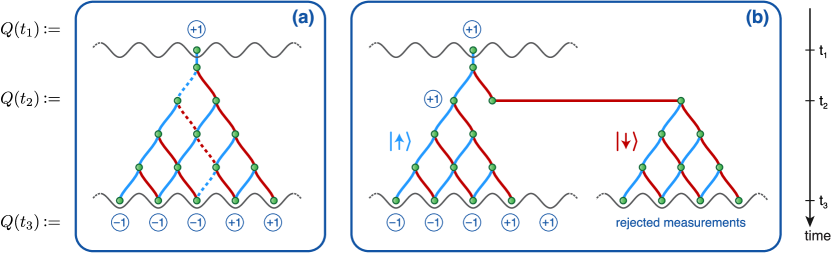
Figure 3: (From Robens et al. (2015)). (a) A Cs atom performs a $4$-step random walk on a $1$D lattice with spin-dependent shifts. (b) The intermediate measurement at $t_{2}$ is an ideal-negative-result measurement: if the atom is has spin down it interacts with the field, is displaced far away and the measurement discarded, otherwise it experiences no interaction.

The experiment worked as follows: a Cs atom with two addressable internal states, $|\!\!\uparrow\rangle$ and $|\!\!\downarrow\rangle$, is controlled via two independent optical lattices. The atom “experiences” only the field of one of the lattices, depending on whether it is in the state $|\!\uparrow\rangle$ or in the state $|\!\downarrow\rangle$.

Therefore, a coherent superposition $(|\!\!\uparrow\rangle+|\!\!\downarrow\rangle)/\sqrt{2}$ follows a quantum random walk, i.e., two independent paths simultaneously, according to a quantum description, whereas it follows a random walk according to a MR description. The atom is then let displace $4$ times, and measurements are performed at $t_{1}=\tau$, $t_{2}=2\tau$ and $t_{3}=4\tau$, where $\tau$ is approximately $26\mu s$; see Fig. 3(a). The LG test works as follows. At step $1$ the atom is just prepared in state $|\!\!\uparrow\rangle$ and at position $x=0$, with a deterministic assignment $\mathsf{Q}(t_{1})=1$. At the intermediate time $t_{2}$ a measurement is performed with an ideal-negative-result strategy: if the atom is in the state $|\!\!\downarrow\rangle$ it experiences one field that displaces it far away and the corresponding result is discarded. In contrast, the atom in the state $|\!\!\uparrow\rangle$ does not experience this shift and it is consequently kept and allowed to further evolve according to the quantum walk until the final measurement at $t_{3}$; see Fig. 3(b). From a macrorealist perspective, the atoms who interact with the field and are discarded are only those in the state $|\!\!\downarrow\rangle$, so the measurement of the state $|\!\!\uparrow\rangle$ is performed in a noninvasive way. The expression Robens et al. consider is

$$W:=\sum_{q_{3}q_{2}}q_{3}p(q_{3}q_{2})-\sum_{q_{3}}q_{3}p(q_{3})\leq 0,$$ (35)

obtained by a specific choice of some trivial measurements in the three-term LGI. Interestingly, this expression closely resembles the inequality version of the NSIT condition. In addition, the authors also estimate the quantum witness $|W|$ Li et al. (2012).

The authors evaluated the macroscopicity measure defined by Nimmrichter et al. in Nimmrichter and Hornberger (2013). Such a measure, called $\mu$, sets a lower limit for the time (expressed in logarithmic scale) during which an electron is delocalized over distances larger than a certain length scale $\ell$, which represents a phenomenological parameter. The value estimated in the experiment is $\mu=\log_{10}(T\hskip 2.0ptM^{2}_{a}/m_{\text{e}}^{2})\approx 6.8$, with $M_{a}$ and $m_{\text{e}}$ being the masses of the Cs atom and of an electron and $T$ being the total duration of the walk. The reference distance is thus set to $\ell=2\mu m$, which is the maximal distance along which the atom is displaced.

The measurement implemented here can indeed be called ideal negative result from a macrorealist perspective. However one needs to rely on the measurement model assumed by the experimenter, i.e., that the system interacts only with one of the two fields, depending on its internal state. Thus, the class of macrorealist theories ruled out by this experiment are those describing the interaction between the field and the atom as a classical version of the quantum one.

III.2.2 Single-photon excitation in macroscopically-separated crystals

A different approach was pursued by Zhou et al. in Ref. Zhou et al. (2015). Note that this experiment has been discussed also in the review Emary et al. (2014). However, since then, the experiment has been updated, and especially further control runs have been made to test the Markovianity assumption on the two basis states. There, an inequality similar to the original LG inequality was tested, which relied on two assumptions different from the traditional macrorealism assumptions. The first assumption is stationarity, meaning that the conditional probabilities of finding the system in state $i$ at time $t+\tau$, conditioned on it being in state $j$ at time $t$, only depends on $\tau$. Second assumption is Markovianity. The systems consists of a single-photon atomic excitation displaced over two spatially separated crystals, whose dynamical evolution is controlled with a polarization-dependent atomic-frequency comb (AFC). This system can be described as a qubit, using a collective Dicke state arising from the absorption of a photon. The two basis states are $|e\rangle=\sum_{j=1}^{N}c_{j}e^{-ikz_{j}}e^{i2\pi\delta_{j}t}|g_{1},\dots,e_{j},\dots,g_{N}\rangle$ and $|g\rangle=|g_{1},\dots,g_{j},\dots,g_{N}\rangle$, where $N$ is the total number of atoms in the comb, $|e_{j}\rangle$ and $|g_{j}\rangle$ are the excited and ground state of the atom in position $z_{j}$. The other parameters are the wave number $k$ of the input field, the detuning $\delta_{j}$ of the atom with respect to the light frequency, and the amplitudes $c_{j}$ which depend on the frequency and on the position of atom $j$.

In the experiment, the system evolves with an oscillatory dynamics between these two basis states. Measurement performed in the qubit basis provide evidence that both stationarity and Markovianity hold. In particular, the authors measured at different times the four conditional probabilities ${p(i,t+\tau|j,t)}$ with $i,j=\{g,e\}$ referring to the two different states, ground and excited, and the evolution is an oscillatory dynamics between them. They also estimated the trace distance between the two basis states as it evolves in time, seeing that it decreases monotonically over time as it should for a Markovian dynamics. Thus, in a sense they tested both assumptions with independent experiments. However, they still rely strongly on the assumption that only two basis states are involved in the dynamics. Then, they tested the inequality $\langle Q(0)Q(2t)\rangle\pm 2\langle Q(0)Q(t)\rangle\geq-1$ by measuring over time the correlations of the dichotomic observable given by $\mathsf{Q}=|g\rangle\langle g|-|e\rangle\langle e|$, observing a sensible violation that follows perfectly the predictions of the quantum mechanical model. Thus, given also the control tests performed, one could argue that the experiment disproves classical theories with two states. Macroscopicity, as quantified by the disconnectivity, is very low ($D=1$) in the experiment, although the excitation was displaced between two macroscopic crystals separated by a length of the millimeter scale.

Figure 4: (From Zhou et al. (2015)). A delocalized atomic excitation is created between two pieces of Nd³⁺:YVO₄ crystals which sandwich a $45^{\circ}$ half-wave plate (HWP). The evolution of the excitation is controlled with a polarization-dependent atomic-frequency comb (AFC). Photon pairs are generated in the PPKTP crystal and then spectrally filtered and separated by the polarization beam splitter (PBS). The H- and V-polarized photons are independently stored in the two pieces of crystals and acquire a different phase shift. After a programmable delay, the polarization of retrieved signal photons is analyzed with a quarter-wave plate (QWP), a HWP and a PBS. Single photon signals are detected with single-photon detectors (SPDs) and analyzed with time interval analyzers (TIA).

III.2.3 Neutrino oscillations

A similar test of LG combined with the assumption of stationarity was performed on neutrino flavor oscillation Formaggio et al. (2016). One additional motivation for this test was that neutrinos can maintain coherence in very large distances due to their low interaction with the environment. In fact, neutrino oscillations were detected after a distance of approximately $735$ km in the data analyzed in Formaggio et al. (2016) and taken from the MINOS collaboration Sousa (2015). In particular, violations of LG inequalities (with the assumption of stationarity) were detected in oscillations between muon and electron-flavored neutrinos, i.e., between the two states $|\nu_{\mu}\rangle$ and $|\nu_{e}\rangle$ treated as a qubit system. The assumption of stationarity as a substitute for noninvasivity was employed in order to sample identically prepared copies of the system rather than a single system evolving in time; technically, the authors analyzed the data at different frequencies, which correspond to different times. In fact, for the case of neutrino oscillations it is impossible to perform sequential measurement, so different assumptions, such as stationarity, are necessary.

III.2.4 Nuclear magnetic resonance

Over recent years, a number of macrorealism tests have been performed using nuclear spin systems, such as Nitrogen-Vacancy centers or Nuclear Magnetic Resonance spectrometers. In particular, two recent experiments appeared Katiyar et al. (2017); Majidy et al. (2019) which used a Bruker DRX $700$MHz spectrometer, where the NMR samples are given by ${}^{13}C$ nuclei of a chloroform molecule, representing the system qubits, probed by ${}^{1}H$ nuclei, playing the role of the ancillary qubits. A prototype dynamics for these experiments, as well as for other macrorealism tests, is given by a rotating spin, i.e., a system governed by the Hamiltonian $H_{S}=\Omega J_{x}$, where $J_{x}$ is the spin operator in a direction $x$ (not necessarily spin-$1/2$) and $\Omega$ is the rotation frequency (cf. Sec. II.1 and Fig. 2). The measurement is performed along the $\mathsf{Q}=J_{z}$ direction through the ancillary spins and in these systems it is typically employed the ideal-negative-result scheme of neglecting the rounds in which a system-ancilla interaction is detected, which is meant to address the clumsiness loophole. However, note that in liquid NMR samples another problem arises typically, which is the fact that the system is extremely noisy, with the preparation typically being $\varrho=\epsilon|0\rangle\langle 0|+(1-\epsilon)\mathbbm{1}$ for $\epsilon\sim 10^{-5}$ or even smaller. This raises the issue of a fair-sampling assumption, which has to be made in such systems; see also Sec. 6 in Ref. Emary et al. (2014) for a discussion about this point. In Katiyar et al. (2017) the experiment followed the idea of Budroni and Emary (2014) of testing macrorealism in multilevel systems and implemented the dynamics of a spin-$1$ system taken from the symmetric triplet subspace of two ${}^{13}C$ qubits. In Majidy et al. (2019) instead, they considered single qubits, but probed several versions of Leggett-Garg inequalities, especially regimes in which violation of macrorealism was detected with only subsets of them Halliwell (2016b). Moreover, they employed the approach of Halliwell (2016a), in which a time-continuous measurement was performed of the velocity $v(t)=\dot{\mathsf{Q}}=\Omega J_{y}$ (so-called waiting detector). With this measurement, they read-off the time integrated quantity $\int_{t_{i}}^{t_{j}}v(t){\mathrm{d}}t=\mathsf{Q}(t_{i})-\mathsf{Q}(t_{j})$ and could thus readily estimate the correlators from the second moments $\langle(\mathsf{Q}(t_{i})-\mathsf{Q}(t_{j}))^{2}\rangle$. As they point out, this measurement scheme allows to substitute the noninvasivity assumption with that of the observable making only one change of sign Halliwell (2016a); Majidy et al. (2019). In the experiment, this was also complemented by an independent set of experiments with the negative-result measurements, in order to provide further evidence of negligible classical disturbance.

III.2.5 Superconducting qubits

Several experiments have been also made with superconducting qubit systems. Knee et al. Knee et al. (2016) performed a macrorealism test that rules out classical models based on $2$-level systems. Concretely, they used a flux superconducting qubit and prepared it in an equal superposition of the two quantum states $|\psi\rangle=(|0\rangle+|1\rangle)/\sqrt{2}$ and afterwards made a projective measurement in the computational basis. Then they performed some runs of the experiment with an additional blind measurement in between (i.e., a measurement without outputs) and evaluated the quantum witness $W$. To exclude classical theories larger than just macrorealism, they performed control experiments calculating the disturbance of the blind measurement in each of the two states $\{|0\rangle,|1\rangle\}$ separately and subtracted from $W$ the value of the largest disturbance. As a result, all interpretations based on classical mixtures of the two computational basis states are excluded, thus ruling out essentially a classical $2$-state model for their intermediate operation.

After this, a number of experiments with superconducting qubits have been implemented using the IBM 5Q Quantum Experience Huffman and Mizel (2017); Ku et al. (2020); Santini and Vitale (2022), which is a system of five superconducting qubits that can be programmed via a publicly accessible website interface IBM . In particular, Huffman and Mizel  Huffman and Mizel (2017) implemented the protocol adroit-measurement protocol developed by Wilde and Mizel Wilde and Mizel (2012); see Fig. 5.

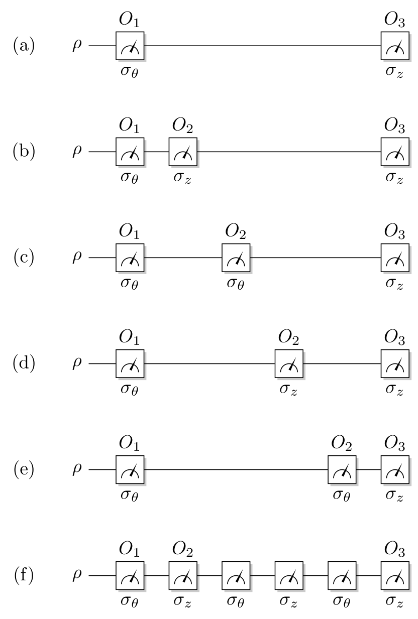
Figure 5: (From Huffman and Mizel (2017)). The target qubit is prepared in an eigenstate of $\sigma_{\theta}$ for $\theta=-3\pi/4$, which corresponds to operation $O_{1}$. Protocol (a) is implemented by performing a measurement in the $\sigma_{z}$ eigenbasis after the preparation $|1\rangle\langle 1|_{\theta}$; for protocols (b) and (d) the state is transferred to a different ancillary qubit with a CNOT gate and then the ancilla is measured in the $\sigma_{z}$ eigenbasis; protocols (c) and (e) work similarly, just with the measurement preceded by a rotation of the state so that $\theta$ will be aligned to $z$. Finally, in protocol (f) all the measurements are implemented by sending sequentially the state of the target qubit to the $4$ different ancillary qubits and making the measurements as in the corresponding protocol (b),(c),(d),(e).

Concretely, the test was performed on one of the qubits, using the others as ancillas for implementing the protocol fulfilling the limitations and constraints of the IBM platform. The protocols (b), (c), (d), and (e), as described in Fig. 5, were used to estimate the adroitness of each intermediate measurement as $\epsilon_{i}=|\langle O_{3}\rangle_{i}-\langle O_{3}\rangle_{a}|$ where $i=\{b,c,d,e\}$ is a label indicating that the average is computed from the corresponding protocol containing one intermediate measurement. The reasoning is then that a violation of the LG inequality $\mathcal{L}:=\langle O_{3}\rangle_{a}+\langle O_{2}\rangle_{f}+\langle O_{2}O_{3}\rangle_{f}+1\geq 0$ with the additional verification that $|\mathcal{L}|\geq\epsilon_{b}+\epsilon_{c}+\epsilon_{d}+\epsilon_{e}$ signals a violation of macrorealism or some sort of collusion between the measurement disturbances.

An upgraded version of the same platform was used by Ku et al. Ku et al. (2020) to perform a macrorealism test preparing at time $t_{1}$ an optical cat states $\cos\tfrac{\theta}{2}|0\rangle^{\otimes n}+\sin\tfrac{\theta}{2}|1\rangle^{\otimes n}$ of $n=2,3,4,6$ qubits and then evolving it to the state $|0\rangle^{\otimes n}$ at time $t_{2}$. The idea is that these states have increasing disconnectivity for increasing $n$. The authors test the violation of an inequality of the form $|W|\leq\mathcal{I}(q=1)$, where the quantum witness is obtained as in Eq. 35 with the measured observable being $\mathsf{Q}=|0\rangle\langle 0|^{\otimes n}$. Here, the additional quantity on the right-hand gives a measure of the invasivity and is given by $\mathcal{I}(q)=|1-p(q|q)|$, where $p(q_{2}|q_{1})$ is the probability that the measurement changes the value of the observable from $q_{1}$ to $q_{2}$. This quantity has been independently measured in order to ensure a non-clumsy violation of macrorealism. In their protocol, the outcome $q=1$ is ideally obtained at $t_{2}$ with certainty if there are no measurements at $t_{1}$. However, when a measurement is performed at $t_{1}$ the ideal probability of observing outcome $1$ becomes $\sum_{q_{1}}p(q_{2}=1,q_{1})=\cos^{4}\tfrac{\theta}{2}+\sin^{4}\tfrac{\theta}{2}$. It is worth noticing here that ideally a higher difference is obtained with the state $\tfrac{1}{\sqrt{2}^{n}}\left(|0\rangle+|1\rangle\right)^{\otimes n}$, which has minimal value of the disconnectivity (and in fact it is just a product state). With this, we emphasize once more the fact that a macroscopically entangled state is not stricly needed for the violation of macrorealism.

III.2.6 Heralded single photons

Finally, experiments were recently also conducted with heralded single photons. In the experiment discussed in Ref. Wang et al. (2018), the idea of Emary Emary (2017) was implemented, namely, that of making ambiguous negative-result measurements on a three-level system. This allows for a replacement of the assumption of NIM with that of EIM, as discussed Sec. III.1. Here, the three levels are encoded in different polarization/path states of one photon, and the measurements are performed to detect coincidences with a trigger photon, which is created in a pair with the target photon through parametric down-conversion. This also has a consequence that not all rounds are valid and thus a fair-sampling assumption has to be employed. In fact, notice that the “measurement” $\{\openone-|q\rangle\langle q|\}_{q}$ is not a POVM, so it must necessarily be implemented via some postprocessing operation, in which the undesired results, in this case a no-detection event, are discarded.

Joarder et al. Joarder et al. (2022) also use heralded single photons, but perform a more traditional LG test; see Fig. 6. This test has the merit of addressing very carefully the loopholes that arise from the detection of the events, in particular, problems such as the imperfect detection efficiency, the emission of multiple photons from the source or from different other sources, and the registration of coincidence events. The clumsiness loophole here is addressed by performing negative-result measurements, and additionally ensuring that all the two-time NSIT conditions like Eq. 27 are satisfied. Thus, in this case the violation of LG inequalities comes from the genuine violation of a three-time NSIT condition. This is the case of $2$-adroit measurements that violate a LGI for sequences of $3$; see also the discussion in Sec. III.1.4. Furthermore, the argument for making classical explanations of the distubance unlikely relies on the fact that measurements of the two different outcomes are performed in spatially well separated regions, which makes it an argument for the experiment to have a nontrivial degree of macroscopicity, in a similar sense as the experiment with neutrinos Formaggio et al. (2016). Note also that the particular case of macrorealism violation in interference experiments has been also discussed in more detail in other recent theoretical works Halliwell et al. (2021); Pan (2020). Similarly as other experiments involving detections of photons (e.g., Zhou et al. (2015)) or neutrinos Formaggio et al. (2016), it was not possible to perform an actual sequence of measurements, but only a single (coincidence) measurement was performed at the end. The different times are then associated to longer paths taken by the photons (cf. Fig. 6).

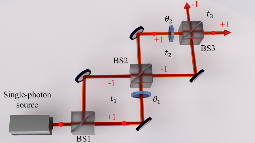
Figure 6: (From Joarder et al. (2022)). Schematic picture of the experimental setup of Joarder et al. (2022). The BS are beam splitters, while the $\theta$ are phase modulators. As indicated in the figure, the two different paths in the interferometers correspond to the two different outcomes and the three time instants correspond to the paths after each BS.

To conclude this section, we note that experimental tests of LGI have significantly improved over the years: an increasing attention has been devoted to the analysis of possible loopholes, with the development of more refined theoretical arguments and experimental implementations. These approaches still rely on some description of the experimental apparatus and the measurement process and some additional assumptions that substitute the strong hypothesis of NIM. Nevertheless, one must admit that there are fundamental limitations in performing a LG test completely removing any assumption on the invasivity of the measurement. These efforts in the design and implementation of more elaborated experiments addressing the loopholes in LG tests contribute to disproving a larger set of macrorealist models, thus providing increasingly stronger arguments against them.

IV Nonclassical temporal correlations beyond noninvasive measurements

IV.1 Operational relaxations of noninvasive measurability

Information processing tasks, classical or quantum, normally involve a series of steps where data is read from a memory, manipulated and written again. The sequentiality of such operations suggests that temporal correlations may play a role in explaining quantum advantages in information processing. However, Leggett-Garg NIM assumption imposes a strong restriction on which tasks can be analyzed: Any classical device with an internal memory that is updated sequentially would violate NIM. A similar drawback holds for the proposals that we have just analized to substitute the NIM assumption with an arguably weaker assumption on the measurement invasivity, which is then tested via control experiments.

In the light of this, a natural way to relax NIM assumption in a systematic way that is suitable for applications in information-theoretic tasks is to allow a bounded internal memory: The operations are allowed to be invasive, but they can modify an internal memory of at most $n$ bits; NIM is recovered for the special case $n=0$. This idea was first proposed by Żukowski Żukowski (2014) in the context of LGIs, and further explored in Budroni et al. (2019). This relaxation can be well formulated in information theoretic terms via a finite-state machine or automaton Paz (2003) a box that receives an input $s_{1}$, produces an output $q_{1}$, then receives another input $s_{2}$ and produces another output $q_{2}$, and so on. It is described in terms of a classical probability as

$$\begin{split}p({\bf q}_{\rm 1\rightarrow n}|{\bf s}_{\rm 1\rightarrow n})=\sum_{r_{0},\ldots,r_{n}}p_{0}(r_{0})p_{\rm T}(q_{1},r_{1},|r_{0},s_{1})\ldots\\ \ldots p_{\rm T}(q_{n},r_{n}|r_{n-1}s_{n}),\end{split}$$ (36)

where $\{r_{i}\}$ are the internal states of the machines, $p_{0}$ their initial distribution, and $p_{\rm T}(q_{i},r_{i},|r_{i-1},s_{i})$ is the probability of emitting the output $q_{i}$ and transition to the internal state $r_{i}$, given that the internal state was $r_{i-1}$ and the measurement setting was $s_{i}$. This model corresponds to a classical model in which the system evolves through a sequence of internal states that are not observed and updated after every measurement. The number of internal states, called also the dimension or the memory of the system, is considered to be finite. Finally, notice that the transition rule $p_{\rm T}(q_{i},r_{i},|r_{i-1},s_{i})$ is fixed throughout the process, i.e., we have time-independent operations.

Figure 7: A device-independent temporal sequence. Boxes are either classical or quantum operations with input $s_{i}$ and output $q_{i}$ that act on a finite amount of states. The initial input can be taken as the vector representing, e.g, the first level $\vec{p}_{0}=(1,\dots,0)$.

When the dimension $d$ is allowed to go to infinity, the set of probabilities generated by such a model can cover the whole AoT polytope Hoffmann et al. (2018), as it happens for quantum models. This is due to the fact that the extreme points of the AoT polytope are reached by deterministic strategies, as discussed in Sec. II.3.2. To implement such strategies, one needs sufficiently many states to store the whole past history at a given point in the sequence.

In contrast, when the number of states $d$ is kept constant, the extreme points of the AoT polytope, for given length and number of inputs and outputs, cannot in general be reached. Consequently, the sets of finite-dimensional quantum temporal correlations is strictly larger than the classical one. This fact can be explicitly witnessed by the violation of LG-type inequalities Budroni et al. (2019, 2021); Vieira and Budroni (2022). The memory resources needed to simulate the extreme points of the AoT polytope, i.e., the minimal number of internal states to reproduce the corresponding deterministic outcome-generation strategy via a classical model, were investigated by Spee et al. Spee et al. (2020a), who showed that it scales at least exponentially in the length $n$. In particular, a general criterion to compute such minimal dimension necessary to simulate the extreme points has been introduced in Spee et al. (2020a), based on the reuse of the internal states to generate an output sequence. It can be introduced via a basic example. Consider the sequence $010101$. It has length 6, no inputs, and two possible outputs. It is clear that it can be generated with probability $1$ by a model with two internal states. Intuitively, the state at each time step fixes (deterministically) the future sequence, so to the same internal state it must correspond the same future. It is clear that in this case there are only two possible futures: (a) generate an alternating sequence starting from $0$ and (b) generate an alternating sequence starting from $1$. The general criterion then counts the number of inequivalent futures associated with an input-output sequence. In the case $n=2$ one obtains that the minimal dimension to reproduce all extreme points of the AoT polytope is given by $d=S+1$ where $S$ is the total number of settings Spee et al. (2020a). This idea has been further developed into the notion of deterministic complexity Vieira and Budroni (2022) defined as the minimal number of internal states necessary to deterministically simulate a sequence $\mathbf{q}$ and denoted as ${\rm DC}(\mathbf{q})$. Differences between classical and quantum correlations, thus, arise for a sequence $\mathbf{q}$ only if $d<{\rm DC}(\mathbf{q})$. Moreover, DC can be efficiently computed in the case of sequences without input Vieira and Budroni (2022).

LG-type inequalities that bound classical and quantum models can then be derived by looking at AoT extreme points that cannot be reproduced deterministically. This was used in Hoffmann et al. (2018) to derive an inequality witnessing the quantum dimension. In Budroni et al. (2019), the case of different theories, i.e., classical, quantum, and generalized probability theories (GPTs) were investigated. For the two-input/two-output scenario one has

$$p(01|00)+p(10|10)+p(10|11)\leq\Omega_{2}^{C}<\Omega_{2}^{Q}<\Omega_{2}^{gbit}=3,$$ (37)

where the classical bound for a single bit $\Omega_{2}^{C}=9/4$ is strictly smaller than the bound for a single qubit $\Omega_{2}^{Q}\sim 2.35570$, and the gbit bound refers to a two-state GPT.

The assumption of a finite number of internal states has been used also in recent experiments Knee et al. (2016); Zhou et al. (2015) to substitute NIM with a weaker assumption. In fact, those are also experiments with two inputs (i.e., “measurement” or “no measurement” at a certain time instant) and two outputs. However, in those experiments the two operations corresponding to the two different inputs are concretely given and independent control experiments were needed to exclude classical theories of a given dimension for those concrete operations. Instead, inequalities like (37) are semi-device-independent Pawłowski and Brunner (2011), namely, they assume nothing about the device except the dimension of the physical system. As such, a violation of the classical bound $\Omega_{2}^{C}$ would imply that there is no possible model for a single bit that can account for the observed probabilities.

In contrast to the standard spatial scenario, in the temporal one classical and quantum correlations can be distinguished even in the case of no inputs (or equivalently, just one input), due to the constraints of time-independent operations. A family of inequalities, each valid for all classical automata of dimension $d$ is given by

$$p(0\dots 01)\leq\Omega^{C}_{d,n},$$ (38)

where the sequence consists of $n-1$ zeros and $1$ one at the end and the bound $\Omega^{C}_{d,n}$ depends on both $d$ and $n$. Here, upper bounds on the value $\Omega^{C}_{d,n}$ can be computed for sequences up to length $20$ and a quantum model that violates this bound can be explicitly constructed Budroni et al. (2021). Intuitively this sequence, called one-tick sequence in analogy with the problem of ticking clocks Erker et al. (2017), is the one requiring the higher dimension to be reproduced deterministically. In fact, the system must “count’ that $n-1$ steps passed, then emit the output $1$. Such a deterministic model requires $n$ states. On the other hand, any sequence of length $n$ can be reproduced deterministically by a machine with $n$ states.

This sequence seems to play a special role among all sequences, as investigated in Vieira and Budroni (2022). The numerical optimizations performed on all sequences with no input and two outputs up to length 10, suggest that the maximum probability for a sequence $\mathbf{q}$ for a model of dimension $d$ is upper bounded by the maximum probability, over models of the same dimension, of the one-tick sequence of length ${\rm DC}(\mathbf{q})$. In addition, the numerics also suggest the existence of a universal upper bound of $1/e$ for all sequences with no input and two outputs, whenever $d<{\rm DC}$. In contrast, even a simple quantum model with a single Kraus operator can reach the algebraic bound $p(0\dots 01)=1$ when $n={\rm DC}=d+1$ and we take the limit of both the length and the dimension going to infinity Vieira and Budroni (2022).

More generally, the idea of using some sort of memory complexity for quantifying the degree of nonclassicality of sequential protocols has appeared also in contexts independent from macrorealism. In particular, the concept of dimension witness, which has been first introduced in the context of Bell nonlocality Brunner et al. (2008), has been extended also to the temporal scenario. One of the first proposals involved a preparation and a (projective) measurement device Wehner et al. (2008), which has been extended in a number of ways, from a dimension witness based on the system’s dynamics Wolf and Perez-Garcia (2009), to prepare-and-measure scenarios Gallego et al. (2010); Bowles et al. (2015), contextuality Gühne et al. (2014) and sequential measurements Sohbi et al. (2021), which stimulated several experimental tests Ahrens et al. (2012); Hendrych et al. (2012); Ahrens et al. (2014); Spee et al. (2020b).

A notion of temporal correlations naturally arise in communication scenarios, such as quantum random access codes (QRACs) Wiesner (1983); Ambainis et al. (1999, 2002); Bowles et al. (2015); Aguilar et al. (2018); Miklin et al. (2020), communication complexity Brassard (2003); Buhrman et al. (2010), or communication cost for simulating Bell nonlocality Pironio (2003); Montina and Wolf (2016); Ringbauer and Chaves (2017). Within this framework, Brierly et al. Brierley et al. (2015) introduced a notion of nonclassical temporal correlations. According to their definition, a temporal correlation $p(\mathbf{q}|\mathbf{s})$ generated by transmitting a $d$-dimensional quantum system through several parties that perform local measurements is nonclassical if its classical simulation requires more than $\log(d)$ classical bits of communication. In other words, whenever a distribution can be generated by transmitting a $d$-dimensional quantum system, but not by transmitting a $d$-dimensional classical system, then such a correlation is nonclassical. To detect these nonclassical temporal correlations, the authors introduce a communication-complexity task called Sequential $n$-point modulo-$(m;d)$ problem. In this task, $n$ parties receive each some initial input, with a promise on the sum modulo $d$ of the inputs and they have to generate an output, with $m$ possible values, satisfying a condition on the total sum modulo $d$ of the outputs. They showed a gap in the amount of communication needed in the classical and quantum setup to solve the problem with probability $1$, thus, providing examples of nonclassical temporal correlations according to the definition given. Here the communication plays the role of the memory previously discussed: the message must be encoded in a classical or quantum memory that is then transmitted.

IV.2 Applications of temporal correlations

We discussed how temporal correlations can be a mean of witnessing the minimal number of internal states, or levels, of a physical system needed to describe a given experiment. This number can be interpreted as the memory, from a more information-theoretical perspective such as that of automata theory. The minimal amount of memory can be different for classical and quantum systems, giving rise to a notion of nonclassical temporal correlations and potential quantum advantages in sequential information processing tasks. A typical question is how much, in terms of classical memory, is the cost of a given task that need sequential operations? This was the motivation of some early works on the subject, including the more abstract introduction of the so-called ontological models Harrigan et al. (2007); Galvão (2009).

For quantum models, the question of the minimal Hilbert space dimension needed to explain some observed set of outcome probabilities $p(a|j,r)$, given preparation $r\in\{1,\dots,m\}$ and measurement input $j\in\{1,\dots,l\}$ was addressed first in Wehner et al. (2008) making a parallel with the QRAC. Note that a similar question was also addressed in Brunner et al. (2008) and subsequent works in the context of spatial correlations.

A different approach was followed in Wolf and Perez-Garcia (2009), where the authors considered a (discretized) temporal evolution of expectation values of observables $\langle A(t)\rangle$ and, under the assumptions of Markovianity and time-homogeneity they proved a lower bound on the Hilbert space dimension $d$ given (i) the number of conserved quantities $D$ under a given evolution and (ii) the number $V$ of linearly independent sequences $v_{t}:=(\langle A(t)\rangle,\langle A(t+1),\dots\rangle)$ for $t\in\mathbb{N}$ (called delayed vectors). Such a bound is given by $D+V\leq d^{2}+1$ and can be always attained by a quantum model. Remarkably, instead, a classical $d$-state model does not necessarily exists that saturates the bound.

Back to the static case, still in the prepare-and-measure scenario, classical and quantum dimension witness resembling the CHSH inequality were derived in Gallego et al. (2010) with bounds $\Omega^{C}_{d}<\Omega^{Q}_{d}$ for the two cases; see also Dall’Arno et al. (2012) for an analysis of their noise-robustness and  Hendrych et al. (2012); Ahrens et al. (2012, 2014) for an implementation in photonic experiments. Later, other dimension witnesses beyond the prepare-and-measure scenario were derived Spee et al. (2020c); Sohbi et al. (2021); Mao et al. (2022). Recently, it has been also observed that dimension witnesses provide also lower bounds on the purity of the pre- and post-measurement states Spee (2020). Another early observation Kleinmann et al. (2011) was that contextual models can be simulated via classical finite-state machines, having thus an associated memory cost. In particular, the case of the Peres-Mermin square Peres (1990); Mermin (1990) was analyzed in detail Kleinmann et al. (2011); Fagundes and Kleinmann (2017), showing a gap between the classical and quantum memory necessary to reproduce the temporal correlations. Moreover several noncontextuality tests involving sequential measurements were translated into proper dimension witnesses Gühne et al. (2014).

A classical ontological model was proposed for quantum computation with magic states (QCM), a model for universal quantum computation Zurel et al. (2020). The operations allowed in the model are the state preparation, including preparation of magic states, Clifford gates, and Pauli measurements. The model can be easily mapped into a model based only on Pauli measurements. The classical model, then, is simply the model for a sequence of Pauli measurements on an $n$-qubit state. The authors essentially find a classical finite-state machine representation for such measurement sequence, as it was to be expected from the result of Sec. II.3.2. Such a model, however, requires a classical state space with dimension scaling exponentially with respect to the number of qubits. It is possible that such a model can be improved, as no argument of optimality was provided.

Temporal correlations were shown to play a central role in the performance of time-keeping devices Erker et al. (2017); Budroni et al. (2021); Woods et al. (2022). Specifically, one can model a clock as a device that ticks at regular time intervals according to a distribution $p(t)$, i.e., the probability of ticking at a background time value $t$. In this model, a notion of accuracy can be given as $R=\mu^{2}/\sigma^{2}$ where $\mu:=\sum_{t=1}^{\infty}tp(t)$ is the mean and $\sigma^{2}:=\sum_{t=1}^{\infty}(t-\mu)^{2}p(t)$ is the variance. $R$ can be interpreted as the average number of ticks after which the clock uncertainty is greater than the interval between two ticks. It has been observed that $R$ is bounded by $O(d)$ and by $O(d^{2})$ for, respectively classical and quantum $d$-state models Budroni et al. (2021); Woods et al. (2022). Here we use a notation for a discrete-time clock, but the continuous limit has been also considered Budroni et al. (2021); Woods et al. (2022). Furthermore, optimal or close-to-optimal classical and quantum models have been investigated for this task, which also triggered subsequent investigations into dimension witnesses based on sequences without inputs Vieira and Budroni (2022). Note, in fact, that such a ticking-clock model can be seen as a machine that has no input (i.e., it is repeated equally at each time step) and two outputs (tick and no-tick).

V Outlook and challenges for the future

Let us conclude this perspective article by discussing the possible future directions of the research on Leggett-Garg macrorealism and temporal quantum correlations. We have seen that the notion of macrorealism arises as a hidden-variable model in the temporal scenario, in analogy with the early works of Bell and Kochen-Specker on local realism and contextuality. As such, many of the techniques developed for these fields, like the correlation polytope approach to the computation of Bell and noncontextuality inequalities, can be applied also to macrorealism. However, macrorealist models have a very peculiar property, namely the possibility of measuring directly the global probability distribution from which all possible observations should arise as marginals. As such, the problem can be straightforwardly solved by checking the NSIT conditions, unless additional limitations are imposed on the sequences of measurements that can be performed; see Sec. II. The question remains open of what the optimal tests are, not only with respect to MR models, but also with respect to quantum violations of LGIs and possibly additional figures of merit, such as quantitative estimates of measurement disturbance and more convoluted measurement procedures that appear when trying to close the loopholes. In particular, in future experiments it would make sense to consider measurements which are more general than projective, and potentially also with different state-transformation rules, and to make model-independent tests, which have the weakest possible assumptions.

Indeed, Leggett-Garg tests are subject to several loopholes, as it happens to Bell and contextuality tests. The hardest condition to verify experimentally is the fact that the measurement is noninvasive. Performing a LG test without the NIM assumption may indeed be fundamentally impossible. However, what can be done and what has been done in experiments is to substitute NIM with some weaker assumption that can be supported by additional experimental evidence. This approach may not provide a complete loophole-free experiment, but it can certainly disprove an increasingly large class of macrorealist models. Recent years have seen a considerable progress in this direction, both from the perspective of theoretical arguments and experimental implementations; see Sec. III.

A systematic approach to the relaxation of the NIM assumption is to use the notion of finite-state machines Hoffmann et al. (2018); Budroni et al. (2019); Spee et al. (2020a), i.e., automata with a finite number of internal states. This approach provides a hierarchical and mathematically well formulated set of conditions able to distinguish between classical and quantum correlations. With this notion, MR models are recovered as a machine with only $1$ internal state. A natural relaxation of this condition consists of models with an increasing number of internal states, which, in the limit of an infinite number of them, are able to simulate all possible temporal correlations; see Sec. IV. Some of the LG experiments already went in this direction, by disproving with extra control experiments a classical model with the same number of states as the quantum model, i.e., typically a classical model with two states was disproved with a qubit experiment. However, these experiments using control tests of invasivity only disprove a particular classical model, i.e., they are not model-independent. Future experiments may consider this direction for tightening the loopholes and disproving an increasing number of MR models.

Inequalities that are valid for all of either classical or quantum models with a certain number of states have been derived theoretically and also tested in some experiments with the purpose of witnessing the dimension of the state space, in a way that is independent of any macrorealist consideration. This kind of approach has also the advantage of finding more concrete applications in other quantum information tasks; see Sec. IV.2).

The problem of the characterization of temporal correlations and sequential quantum information processing tasks can be addressed in the more general framework of spatiotemporal correlations. For instance, spatiotemporal correlations can be described via the quantum comb formalism Chiribella et al. (2009), when events have a well-defined temporal order, or the process matrix formalism  Oreshkov et al. (2012); Chiribella et al. (2013) when they do not. These approaches try to capture a general notion of quantum process that involves a multi-partite and multi-time scenario, and in general can weaken the assumption of causality, intended as a definite time-ordering of the events. See also Costa et al. (2018) for an approach that tries to unify the notion of spatial and temporal quantum correlations within this framework. Similarly, macrorealist models can be generalized to more complex sets of causal relations, described by Bayesian networks Pearl (2009). Some recent research in this direction attempts to relax some of the LG assumptions and substitute them with some limitations on the causal influences between classical variables Ringbauer and Chaves (2017).

Furthermore, we mention that temporal correlations are intimately connected to the problem of non-Markovian dynamics. Several works explored these connections Chen et al. (2016); Milz et al. (2020) and assumptions of Markovianity play a role in experimental tests of macrorealism Zhou et al. (2015). Similar assumptions are also used in the context of dimension witnesses Wolf and Perez-Garcia (2009) . These results elucidate to some extent the connections between Markovianity, supplemented by stationarity (i.e., loosely speaking time-translation invariance) and the original LG formulation of macrorealism. Moreover, they can be similarly related to finite-state automata with just a single state. At the same time, the investigations around the notion of Markovianity are far wider Rivas et al. (2014); Breuer et al. (2016); Milz and Modi (2021) and the precise relation with macrorealism has not been explored in full detail, especially in the light of the latest developments in both fields. As a potential outlook, the concept of Markovianity can turn out to be crucial also for extending the notion of temporal hidden variable theories to the case of systems with an infinite number of internal state. Similarly, one can look at a definition of automata with an unlimited number of states. In other words, the notion of finite memory, in terms of a state space ($n$ states), could be substituted with the notion of a finite memory in terms of a time interval ($n$ time-steps). In this scenario, it is still an open challenge to make a meaningful and perhaps operational distinction between classical and quantum models for a sequential scenario.

Another important challenge is to explicitly characterize temporal correlations as resources for specific quantum information processing tasks, such as phase estimations, quantum computation or the classical simulation of a sequence of quantum operations. A natural question, for instance, is whether the classical model of Zurel et al. Zurel et al. (2020) can be optimized to further reduce the number of classical states necessary for the simulation of quantum computation and what is the minimal number. An answer to this question may have important consequences for our understanding of quantum advantages in computation.

Finally, these quantum information applications provide a further motivation for conducting increasingly elaborated LG tests. The finer control of quantum systems over many degrees of freedom, possibly even at some macroscopic level, and over sequences of operations, developed to address the loopholes in LG tests, may turn out to be crucial for the realization of sequential information processing tasks inspired by the study of temporal correlations. At the same time, efforts in that direction are also required to tackle further foundational questions, as well as for new technological developments, such as better sensors, communication networks or quantum computers.