Simulation-based Testing of Simulink Models with Test Sequence and Test Assessment Blocks

Abstract

Simulation-based software testing supports engineers in finding faults in Simulink^® models. It typically relies on search algorithms that iteratively generate test inputs used to exercise models in simulation to detect design errors. While simulation-based software testing techniques are effective in many practical scenarios, they are typically not fully integrated within the Simulink environment and require additional manual effort. Many techniques require engineers to specify requirements using logical languages that are neither intuitive nor fully supported by Simulink, thereby limiting their adoption in industry.

This work presents HECATE, a testing approach for Simulink models using Test Sequence and Test Assessment blocks from Simulink^® Test^TM. Unlike existing testing techniques, HECATE uses information from Simulink models to guide the search-based exploration. Specifically, HECATE relies on information provided by the Test Sequence and Test Assessment blocks to guide the search procedure. Across a benchmark of $16$ Simulink models from different domains and industries, our comparison of HECATE with the state-of-the-art testing tool S-Taliro indicates that HECATE is both more effective (more failure-revealing test cases) and efficient (less iterations and computational time) than S-Taliro for $\approx$94% and $\approx$81% of benchmark models respectively. Furthermore, HECATE successfully generated a failure-revealing test case for a representative case study from the automotive domain demonstrating its practical usefulness.

1 Introduction

Engineers often use Simulink^® [1] to design and demonstrate software behavior [2, 3]. It offers a graphical programming environment to simulate and generate code from graphical models. Simulink is used across industries including medical, avionics, and automotive [4, 5]. Techniques that support verification of Simulink models, a significant and widely recognized software engineering problem [6, 7], are of interest to academia and industry alike. There are many techniques to verify Simulink models including formal methods and simulation-based software testing [8].

Formal methods tools such as Simulink^® Design Verifier^TM [9], FRET [10], and QVtrace [11] support verification of Simulink models. For example, Simulink Design Verifier uses formal verification for detection of design errors (e.g., division-by-zero), identification of dead logic, generation of test cases to ensure some amount of test coverage, and exhaustive verification of properties capturing system requirements. Formal methods tools typically have constraints on the kinds of Simulink models that can be analyzed [12]. For example, Simulink Design Verifier runs a compatibility check before its execution [13] and cannot perform verification on incompatible models. In contrast, simulation-based software testing, the technique considered by this work, does not impose restrictions on the kinds of Simulink models that can be analyzed.

Simulation-Based Software Testing, a widely used technique to test Simulink models [8], relies on simulations to detect software failures. Simulation test cases are either manually specified by the user (e.g., [14, 15, 16]) or are automatically generated (e.g., [6, 17, 18, 19, 20, 21, 22, 23]).

Manual test case specification requires engineers to manually specify test inputs and assessment procedures to verify whether requirements are satisfied or violated. This approach is largely used in the industrial domain [24] and is mandated by safety standards [25]. Manual test case specification is supported in Simulink^® Test^TM [26] via the Test Sequence block that lets users construct complex test inputs [27], and the Test Assessment block that lets users specify the procedure to check the requirements of interest [28]. Manual test case specification builds on human capabilities (e.g., domain knowledge) to define test cases. However, the manual definition of test cases is a laborious task especially for large-scale industrial projects [22]. Therefore, there is a need for automated support to alleviate some of the manual effort.

Automated test case generation entails automatic generation of test cases [8]. For example, falsification-based testing tools for Simulink models iteratively explore the input space to detect failure-revealing test cases (e.g. [6, 17, 18, 19, 20]). Falsification-based testing tools for Simulink models include Aristeo [6], Breach [29], FalCAuN [30], falsify [31], FalStar [32], ForeSee [33], and S-Taliro [34]. However, these tools are not based on native Simulink Test blocks that are often used by industry practitioners. They also require engineers to specify requirements and input profiles using formal languages (e.g., Signal Temporal Logic [35])—a time-consuming and error-prone task, as widely recognized by the software engineering community [36, 37]. This limitation makes the application of falsification-based techniques laborious and hinders their use in industrial applications. For this reason, this paper proposes an automated test case generation technique that supports Test Sequence and Test Assessment blocks (together referred to as Test Blocks for brevity in the rest of the paper).

To summarize, the problem addressed by this work is to support automation of test case generation from manual test case specifications done using Simulink Test Sequence and Test Assessment blocks.

To address this problem, we present HECATE, a Test Sequence and Test Assessment driven Approach for Simulink models. HECATE bridges the gap between manual test case specification and automated test case generation. Specifically, HECATE is the first simulation-based software testing approach that supports Test Blocks. On the one hand, unlike existing automated test case generation techniques, HECATE leverages manual test case specification artifacts (Test Blocks) to guide the search-based exploration. On the other hand, unlike existing manual test case generation techniques, HECATE also systematically automates the generation of test cases.

HECATE requires engineers to extend their test sequences into Parameterized Test Sequences: test sequences augmented with a set of parameters and their domains. These Parameterized Test Sequences define the universe of test sequences to be considered during the search. HECATE automatically searches for parameters values that lead to test sequences that show a violation of the conditions specified by the Test Assessment block. To enable the search, HECATE provides a procedure that automatically converts Test Assessment blocks into fitness functions. HECATE is implemented as a plugin for S-Taliro [34], a widely known testing tool for Simulink models.

To evaluate effectiveness and efficiency of HECATE, we identify (a) a baseline tool, and (b) a benchmark for our comparison. For the baseline tool, we use S-Taliro. Unlike HECATE, S-Taliro requires Signal Temporal Logic (STL) [35] specifications and input profiles to describe the requirement to be considered and the search domain (together referred to STL artifacts in the rest of the paper). As part of the contribution of this work, we propose a new benchmark of $16$ Simulink models that includes both Test Blocks and STL artifacts. The benchmark includes models from an international competition on falsification-based testing tools [38], from the web ([39, 27, 40, 41, 42, 43]), and includes models developed by Toyota [44] and Lockheed Martin [45, 46]. Our results show that for our benchmark models, HECATE is more effective than S-Taliro in finding failure-revealing test cases for $\approx$94% of the models. HECATE was also more efficient than S-Taliro for $\approx$81% of the models. To evaluate the applicability of HECATE, we selected a large and representative automotive case study developed by MathWorks in the context of the EcoCAR Mobility Challenge [47], a competition they jointly organize with the U.S. Department of Energy and General Motors. We check whether HECATE could generate a failure-revealing test case. HECATE successfully returned a failure-revealing test case for our case study.

To summarize, our contributions are as follows:

• HECATE, a testing approach for Simulink models with Test Blocks (Section 3);

• the use of Parameterized Test Sequences (Section 4.1);

• compilation of Test Assessment blocks into fitness functions (Section 4.2);

• a benchmark of $16$ Simulink models that include both Test Blocks and STL artifacts (Section 6.1);

• effectiveness and efficiency assessment of HECATE by comparing it with S-Taliro (Section 6.2 and Section 6.3);

• applicability assessment of HECATE on a representative case study from the automotive industry (Section 6.4);

• and a complete replication package.

The structure of this paper is as follows: Section 2 introduces Test Sequence and Test Assessment blocks. Section 3 presents HECATE. Section 4 and 5 describe the two main phases of HECATE: the driver and the search phases. Section 6 evaluates our contribution. Section 7 discusses our results and threats to validity. Section 8 presents related work. Section 9 concludes summarizing our results.

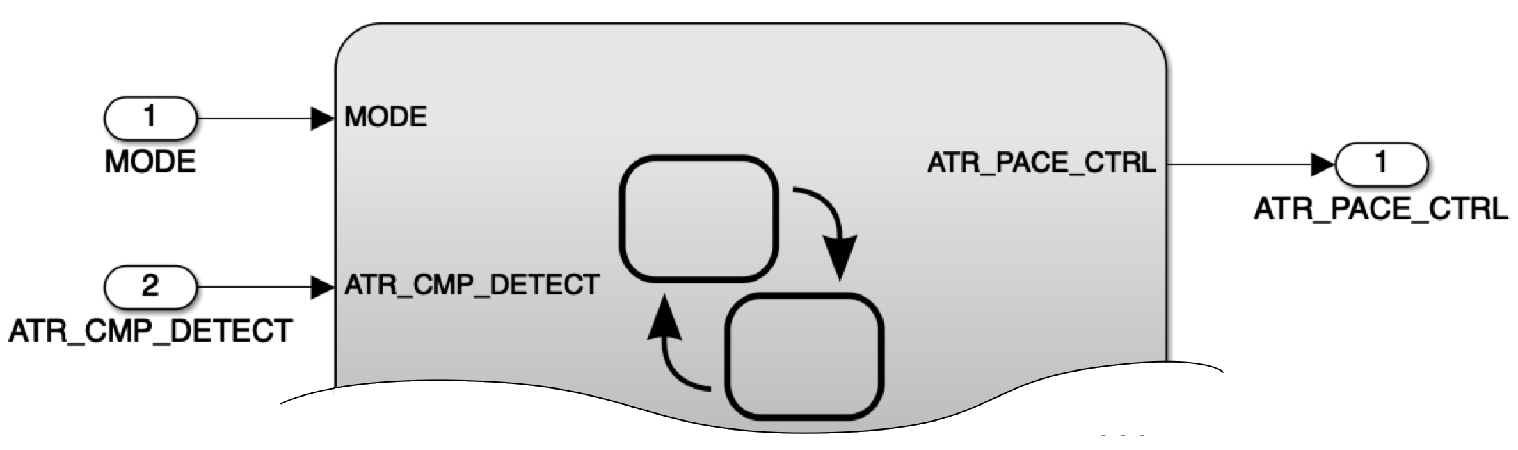
Figure 1: A portion of the Simulink^® model of a pacemaker controller.

2 Background and Running Example

This section describes an illustrative example of a pacemaker model [39] to informally introduce the syntax and semantics of Test Blocks.

A pacemaker is a medical device that regulates its user’s heart rate. Its control software can be designed using Simulink. Figure 1 depicts a portion of the controller model. The pacemaker is connected to the heart atrium and ventricle using sensors to check heart activity and actuators to deliver electrical signals for muscle activation. The portion of the Simulink subsystem (gray box) shown in Figure 1 includes input ports MODE and ATR_CMP_DETECT and an output port ATR_PACE_CTRL. Input signals from these input ports are the desired operational mode for the pacemaker and a signal that specifies how the atrial pulse from the heart is detected, respectively. The output signal to the output port indicates whether the atrium should be paced.

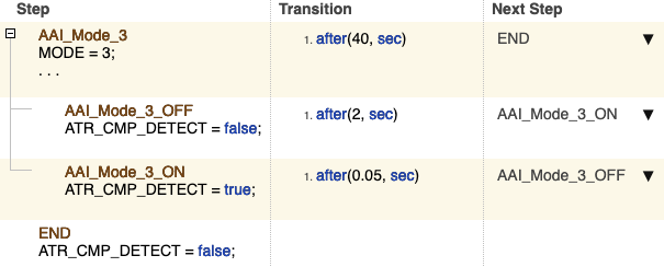
(a) Test Sequence

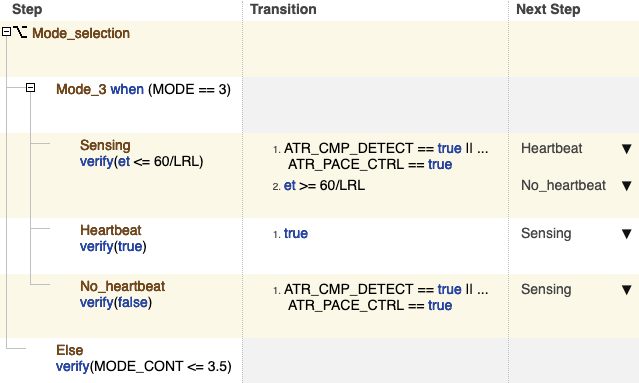
(b) Test Assessment

Figure 2: Simulink^® Test Sequence and Test Assessment blocks for the pacemaker example.

Figure 2 presents portions of Test Sequence and Test Assessment blocks for the pacemaker example that introduce the syntax and semantics of these two block types [48]. Test Blocks are comprised of test steps connected by transitions. The Test Sequence block in Figure 2a and the Test Assessment block in Figure 2b contains four (AAI_Mode_3, AAI_Mode_3_OFF, AAI_Mode_3_ON, END) and six (Mode_selection, Mode_3, Sensing, Heartbeat, No_heartbeat, Else) test steps respectively. Test steps are hierarchically organized. For example, the test step Sensing of Figure 2b is nested within the test step Mode_3. At each time instant, the Test Blocks are in exactly one ‘leaf’ test step and its ‘ancestors’ in the hierarchy. For example, if the Test Assessment in Figure 2b is in the leaf test step Sensing, it is also in all of its ancestors, namely Mode_3 and Mode_selection. Whenever a Test Block enters a ‘non-leaf’ test step, it also enters its first child test step. For example, if the Mode_3 test step of Figure 2b is entered, the test step Sensing is also entered.

Transitions define how a Test Block switches between test steps. For example, transitions of the Test Assessment block from Figure 2b specify how the Test Assessment switches between the test steps Mode_selection, Mode_3, Sensing, Heartbeat, No_heartbeat, and Else. Whenever a non-leaf test step is exited, so are all of its ‘descendants’. For example, if the Test Assessment of Figure 2b is in the test step Sensing and the value of the MODE changes to the value $2$, the Mode_3 test step is left and the test step Sensing is also left. Two precedence rules regulate the firing of transitions: First, if two transitions associated with test steps at the different levels of the hierarchy are active at the same time instant, the transition at the highest level of the hierarchy is fired. Second, if two transitions associated with the same test step become active, the first among the defined transitions is fired. Transitions are classified as standard transitions and when decompositions.

Standard transitions connect a source and a destination test step. They are labelled with a Boolean formula representing a condition for the transition to be fired. The formula is defined using transition operators, temporal operators, and relational operators summarized next (see [48] for additional information).

1. Transition operators return Boolean values and evaluate the occurrence of signal events. For example, the transition operator hasChanged(u) detects if signal u changed its value compared to the previous timestep.

2. Temporal operators return values providing timing information related to a Test Block. For example, the temporal operators after(n, TU) and et(TU) respectively evaluates if n units of time have elapsed since the beginning of the current test step, and retrieves the time elapsed from since a test step is entered.

3. Relational operators ($<,\leq,>,\geq,=$) compare the values of arithmetic expressions defined on the values assumed by signal inputs, parameters, or constants. Arithmetic expressions can be defined by using arithmetic and temporal operators.

As an example, the standard transition from the test step AAI_Mode_3 to the test step END in Figure 2a is associated with the condition after(40, sec) which becomes true after the system has been in the test step AAI_Mode_3 for $40$s.

When decomposition corresponds to switch statements from programming languages. For example, the when decomposition of the Test Assessment block in Figure 2b specifies that the Test Block is in the test step Mode_3 depending on whether the value assumed by the variable MODE is $3$.

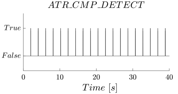
(a) Test Input

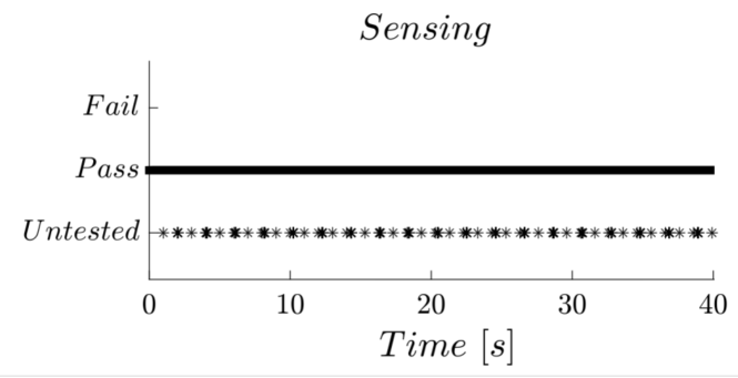
(b) Test Output

Figure 3: Input signal generated by the Test Sequence of Figure 2a and output signal of the Test Assessment of Figure 2b.

Test steps from Test Sequence and Test Assessment blocks differ in their purpose in the following manner. In Test Sequences, they define the values assumed by the input signals. For example, the test steps AAI_Mode_3_OFF and AAI_Mode_3_ON of the Test Sequence of Figure 2a assign the values false and true to the variable ATR_CMP_DETECT, respectively. In contrast, in Test Assessment, they contain verification statements, i.e., verify and assert, which check whether a logical expression evaluates to true or false. For example, the statement verify(et$<$60/LRL) of the test step Sensing in Figure 2b checks whether or not the pacemaker spends less than 60/LRL seconds sensing for a heartbeat. The lower rate limit LRL changes depending on the user activity, e.g., sleeping, running. Differently from the verify statement, the assert statement also stops the simulation if the logical expression evaluates to false.

A test case is made of a Test Sequence block and a Test Assessment block. For example, the Test Sequence and Test Assessment blocks in Figure 2 form a test case for the Simulink model of Figure 1.

The Test Sequence block generates a test input containing one input signal for each input port. For example, Figure 3a presents an input signal for the input port ATR_CMP_DETECT from the Test Sequence block in Figure 2a. The input signal ATR_CMP_DETECT of the test input reported in Figure 3a repeatedly changes its value between true and false following the specification of the Test Sequence block from Figure 2a. More specifically, the Test Sequence block switches from AAI_Mode_3_OFF to AAI_Mode_3_ON every $2$s, and vice versa every $0.05$s. Therefore, the value of the signal ATR_CMP_DETECT (Figure 3a) switches between false to true every $2$s, and vice versa every $0.05$s. The test input is then executed by simulating the model for the input signals associated with the Test Sequence.

Test Assessment block evaluates if the output signals of the model lead to a violation of the expressions of its verify and assert statements. It produces an output signal for each verify and assert statement. For example, Figure 3b presents the output signal produced by the verify statement of the Sensing test step from the Test Assessment block in Figure 2b. For each time instant, the value of the output signal is computed as follows. If the Test Assessment is not in the Sensing test step, the output signal is marked Untested. Otherwise it is assigned a value of Pass or Fail, depending on whether the logical expression contained within the verify statement is true or false. In our example, the value for this statement is always Pass since the Test Assessment either moves to the test step Heartbeat or No_heartbeat before the condition et$<$60/LRL evaluates to false. A verification statement (verify or assert) is violated if its logical expression evaluates to false at least once, i.e., the output signal is false for at least one simulation step. A test case (Test Sequence plus Test Assessment) is considered a failure-revealing test case for the model if it violates a verification statement.

Despite the large support provided by existing tools for testing Simulink models (see Section 1), none of them can automatically generate Simulink test cases from manual test case specifications defined using Test Sequence and Test Assessment blocks. This lack of support is a significant limitation for practical applications. In the next section, we present HECATE, a systematic framework that overcomes this limitation by using manual test case specification to automatically generate new failure-revealing test cases.

output = [coordinate]

[auto, block/.style =rectangle, draw=black, thick, fill=white!20, text width=5em,align=center, rounded corners, block1/.style =rectangle, draw=blue, thick, fill=blue!20, text width=5em,align=center, rounded corners, minimum height=2em, line/.style =draw, thick, -latex’,shorten ¿=2pt, cloud/.style =draw=red, thick, ellipse,fill=red!20, minimum height=1em]

(0,0) node[block] (Input) [baseline=(X.base)][draw=black,fill=white,thick,rectangle,inner sep=2pt, rounded corners=2pt](X)3; Input
Generation; [output, right of=Input,node distance=1.7cm] (InputMiddle) ; [block, below of=InputMiddle,node distance=0.3cm,text width=6.5cm,minimum height=2.1cm,dashed,draw opacity=1] (Search) ;

(0,0) node[block] (InputRef) [baseline=(X.base)][draw=black,fill=white,thick,rectangle,inner sep=2pt, rounded corners=2pt](X)3; Input
Generation;

[block, above of=InputMiddle,node distance=2.4cm,text width=6.5cm,minimum height=2.05cm,dashed] (Driver) ;

[block, right of=Input,node distance=3.5cm] (Fitness)[baseline=(X.base)][draw=black,fill=white,thick,rectangle,inner sep=2pt, rounded corners=2pt](X)4; Fitness
Assessment;

[output, right of=Fitness,node distance=2.5cm] (uoutput) ; [block, above of=Fitness,node distance=2.2cm,text width=2.2cm] (TestAssessment) [baseline=(X.base)][draw=black,fill=white,thick,rectangle,inner sep=2pt, rounded corners=2pt](X)2; Test Assessment to Fitness Function; [block, above of=Input,node distance=2.2cm,text width=2.2cm] (TestToInput) [baseline=(X.base)][draw=black,fill=white,thick,rectangle,inner sep=2pt, rounded corners=2pt](X)1;
Definition of the Search Space ; [output, above of=TestToInput,node distance=1.7cm] (testsequence) ; [output, above of=TestAssessment,node distance=1.7cm] (testassessment) ; [output, below of=Fitness,node distance=1cm] (loopa) ; [output, below of=Input,node distance=1cm] (loopb) ; (0,0) node [above of=Driver, node distance=0.8cm] (DriverText) Driver Phase; (0,0) node [below of=Search, node distance=0.9cm] (SearchText) Search Phase; [output, right of=Fitness,node distance=0.5cm] (modela) ;

[output, below of=modela,node distance=1.8cm] (model) ; [output, below of=modela,node distance=0.5cm] (modelb) ;

[-stealth] (model.east) – (modelb.south) node[ pos=0.2, right]M; [-stealth] (Input.east) – (Fitness.west) node[midway,above]$\textsc{TS}\_\textsc{c}$; [-stealth] (testsequence.south) – (TestToInput.north) node[near start,right]TS; [-stealth] (TestToInput.south) – (Input.north) node[midway,right]SP; [-stealth] (testassessment.south) – (TestAssessment.north) node[near start,right]TA; [-stealth] (TestAssessment.south) – (Fitness.north) node[midway,right]FF; [-] (Fitness.south) – (loopa.north) node[midway,right]; [-] (loopb.south) – (loopa.north) node[midway,above]$\langle\textsc{TS}_{1},\textsc{f}_{1}\rangle$,$\langle\textsc{TS}_{2},\textsc{f}_{2}\rangle$, …; [-stealth] (loopb.north) – (Input.south) node[midway,right]; [-stealth] (Fitness.east) – (uoutput.west) node[midway,above]TC/NFF;

Figure 4: Overview of HECATE.

3 Test Sequence and Assessment Driven Testing

Figure 4 presents an overview of HECATE. The inputs are the Test Sequence (TS) and Test Assessment (TA) blocks and the Simulink model under test (M). The output is either a failure-revealing test case (TC) or the value NFF (No Fault Found) indicating that HECATE could not detect a failure-revealing test case within the allotted time budget. HECATE is composed of a driver phase and a search phase.

The driver phase compiles the Test Blocks into artifacts that drive the simulation-based search in two steps. Step [baseline=(X.base)][draw=black,fill=white,thick,rectangle,inner sep=2pt, rounded corners=2pt](X)1; defines the search space (SP) associated with the Test Sequence block. Step [baseline=(X.base)][draw=black,fill=white,thick,rectangle,inner sep=2pt, rounded corners=2pt](X)2; translates the Test Assessment block into a fitness function (FF) that guides the search.

The search phase implements the iterative testing procedure of the simulation-based software testing framework in two steps. Step [baseline=(X.base)][draw=black,fill=white,thick,rectangle,inner sep=2pt, rounded corners=2pt](X)3; iteratively generates new candidate Test Sequences ($\textsc{TS}\_\textsc{c}$) using the search space definition (SP). Step [baseline=(X.base)][draw=black,fill=white,thick,rectangle,inner sep=2pt, rounded corners=2pt](X)4; executes the model (M) for the test inputs specified by the candidate Test Sequence. It checks using the fitness function (FF) whether the Test Assessment is satisfied or violated.

The tool stops either by returning the failure-revealing test case (TC) if a violation is detected, or if the computation exceeds its allotted time budget (NFF). Otherwise, it proceeds with a new iteration and step [baseline=(X.base)][draw=black,fill=white,thick,rectangle,inner sep=2pt, rounded corners=2pt](X)3; uses the previously generated test sequences and their fitness values (i.e., $\langle\textsc{TS}_{1},\textsc{f}_{1}\rangle$,$\langle\textsc{TS}_{2},\textsc{f}_{2}\rangle$) to generate a new candidate Test Sequence ($\textsc{TS}\_\textsc{c}$).

Driver and Search Phases are detailed in Sections 4 and 5.

4 Driver Phase

This section describes the two steps of the driver phase: Definition of the Search Space (Section 4.2) and Test Assessment to Fitness Function Conversion (Section 4.1).

4.1 Definition of the Search Space

In step [baseline=(X.base)][draw=black,fill=white,thick,rectangle,inner sep=2pt, rounded corners=2pt](X)1; users amend the Test Sequence to define the search space, i.e., the universe of test sequences to be considered by HECATE for test case generation. Specifically, HECATE requires engineers to (a) create a Parameterized Test Sequence, and (b) define domains for the parameters.

Creating a Parameterized Test Sequence. To create a Parameterized Test Sequence engineers extend a Test Sequence by manually introducing search parameters. Search parameters are variables named with identifiers starting with the string “Hecate” that can be used as Simulink variables. For example, Figure 5a reports a Parameterized Test Sequence with search parameters Hecate_HEARTFAIL, Hecate_DELAYON and Hecate_DELAYOFF for the Test Sequence from Figure 2a.

Definition of parameter domains. Software engineers define parameter domains by providing lower and upper bound values. For example, Figure 5b sets the values $20$ and $60$ as lower and upper bounds for the parameter Hecate_HEARTFAIL.

Parameterized Test Sequences and parameter domains define the search space (SP) of the testing algorithm and are provided as input to the search phase.

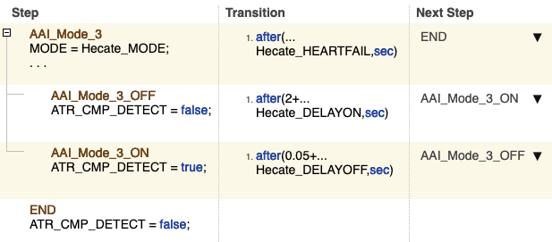
(a) Parameterized Test Sequence

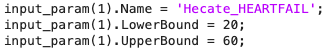
(b) Parameter Domain

Figure 5: Parameterized Test Sequence (Figure 5a) and parameter domain (Figure 5b) for the Test Sequence from Figure 2a.

4.2 Test Assessment to Fitness Function Conversion

Step [baseline=(X.base)][draw=black,fill=white,thick,rectangle,inner sep=2pt, rounded corners=2pt](X)2; converts the Test Assessment into a fitness function (FF) that guides the search procedure. The fitness function needs to ensure the following: (i) a negative fitness value indicates that the property is violated; (ii) a positive fitness value indicates that the property is satisfied; (iii) the higher the positive fitness value is, the farther the system is from violating the property; and (iv) the lower the negative value, the farther the system is from satisfying the property.

The function TA2FF (Test Assessment to fitness function) from Figure 6 implements Step [baseline=(X.base)][draw=black,fill=white,thick,rectangle,inner sep=2pt, rounded corners=2pt](X)2;. It takes a Test Assessment block (TA) as input and returns a Simulink subsystem (FF) representing the fitness function. For example, Figure 7 presents the fitness function generated for the Test Assessment block from Figure 2b. The TA2FF algorithm proceeds as follows. Line 2 creates the FitnessFunction (FF) subsystem (Figure 7a). Line 4 creates its two subsystems: the FITNESS_CONVERTER (FC) and the AGGREGATOR (AG). The FITNESS_CONVERTER has the same input ports as the Test Assessment block, and one output port for each verification statement (verify and assert). Each output port returns the fitness value associated to the corresponding verification statement. For example, the subsystem FITNESS_CONVERTER in Figure 7a has four output ports, one for each of the verification statements from Figure 2b. The output port FIT_SENSING is associated to the statement verify(et$<$60/LRL). The AGGREGATOR subsystem computes a single fitness value from the fitness values of the output ports of the FITNESS_CONVERTER subsystem.

1:  function TA2FF (TA)

2:        FF=createFitnessFunction();

3:        [FC,AG]=initialize(FF);

4:        FC.createStateflow();

5:        FC.createStates(TA);

6:        FC.createTransitions(TA);

7:        FC.addFitnessComputation(TA);

8:        AG.addMinCalculation(SS);

9:        AG.addFeedback(SS);

10:       return FF;

11:  end

Figure 6: The TA2FF algorithm.

To generate the FITNESS_CONVERTER (Figure 7b) Algorithm 6 creates a Stateflow^® chart [49] that mimics the behaviors of the test steps. Line 4 creates an empty Stateflow chart. Line 5 creates the states of the Stateflow chart: one for each test step of the TA nested according to the test steps as necessary. For example, the state No_heartbeat of the Stateflow chart in Figure 7b corresponds to the test step No_heartbeat from Figure 2b and is nested within the state Mode_3 as the test step of the Test Assessment block is nested within the test step Mode_3. Line 6 adds the transitions to the FITNESS_CONVERTER chart by analyzing each transition of the Test Assessment block. If the transition is a standard transition, the algorithm adds a transition to the Stateflow chart of the FITNESS_CONVERTER with the same condition that connects the Stateflow states associated with the source and destination test steps of the transition of the Test Assessment. For example, the transition of the Test Assessment in Figure 2b connecting the test step No_heartbeat to Sensing translates into the transition of the Stateflow chart from Figure 7b connecting the state No_heartbeat to Sensing. If a transition is a when decomposition, the algorithm adds to the Stateflow chart a junction node and two transitions for each when statement: one transition connecting the junction node to the Stateflow state corresponding to the test step of the Test Sequence that is the target of the when statement, and another transition with the opposite source and destination states. The first transition is guarded with the condition of the when statement. The second is associated with the negation of that condition or the satisfaction of the when statement of any of the previous states. Lastly, Line 7 translates the arithmetic expression within each verification statement into a fitness metric. We use the robustness [50] fitness metric since it is widely used for search-based testing (e.g., [17, 19, 6]).

To generate the AGGREGATOR subsystem (Figure 7c) Algorithm 6 proceeds as follows. Line 8 adds a min Simulink block to the AGGREGATOR subsystem that computes the minimum value assumed by the signals of its input ports. For example, the Min block of the AGGREGATOR subsystem (Figure 7c) generated for the Test Assessment from Figure 2b is connected to the input ports FIT_HRTBT, FIT_NOHRTBT, FIT_MODE, and FIT_SENSING. Finally, Line 9 creates a feedback loop with a delay block (to capture the minimum value at the previous time) to compute the minimum fitness value over the entire simulation.

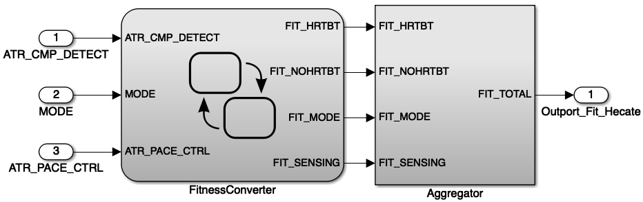
(a) Model of the FITNESS_FUNCTION subsystem (FF).

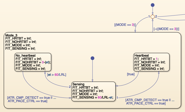
(b) FITNESS_CONVERTER subsystem (FF).

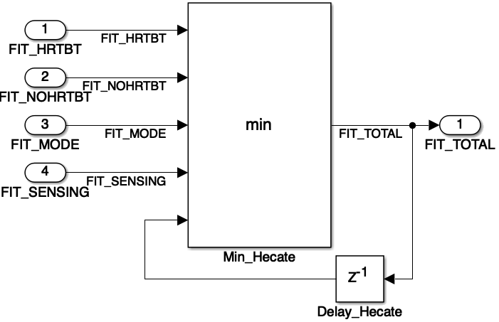
(c) AGGREGATOR subsystem (AG).

Figure 7: Fitness Function generated for the Test Assessment block from Figure 2b.

5 Search Phase

This section describes the two steps of the search phase: Input Generation (Section 5.1) and Fitness Assessment (Section 5.2).

5.1 Input Generation

Input Generation (step [baseline=(X.base)][draw=black,fill=white,thick,rectangle,inner sep=2pt, rounded corners=2pt](X)3;) takes as inputs the search space definition (SP) as well as the Test Sequences previously generated by HECATE ($\textsc{TS}_{1}$, $\textsc{TS}_{2}$, …) and their fitness values (f₁, f₂, …). It generates a new candidate Test Sequence ($\textsc{TS}\_\textsc{c}$) by assigning values to the parameters of the Parameterized Test Sequence within their domains. For example, the Test Sequence from Figure 2a is obtained by assigning the value 0 to all its parameters from the Parameterized Test Sequence from Figure 5a.

HECATE reuses S-Taliro [34] to generate parameters values. We selected S-Taliro since it offers a set of search algorithms, such as Simulated Annealing [51], Monte Carlo [52], and gradient descent methods [53]. HECATE assigns parameters values computed by S-Taliro to the Parameterized Test Sequence. For example, the Test Sequence presented in Figure 2a is a possible Test Sequence returned by HECATE.

5.2 Fitness Assessment

The Fitness Assessment (step [baseline=(X.base)][draw=black,fill=white,thick,rectangle,inner sep=2pt, rounded corners=2pt](X)4;) computes the fitness value for a Test Sequence. This step executes the Simulink model augmented with the FITNESS_FUNCTION subsystem by invoking the sim command [54]. It then extracts the fitness value for the Test Sequence as the last value assumed by the output signal FIT_TOTAL.

6 Evaluation

This section empirically evaluates HECATE by answering the following research questions:

• How effective is HECATE in generating failure-revealing test cases? (Section 6.2)

• How efficient is HECATE in generating failure-revealing test cases? (Section 6.3)

• How useful is HECATE in generating failure-revealing test cases for a large automotive model? (Section 6.4)

To answer RQ1 and RQ2, we compared HECATE with a baseline framework from the literature. Since we are not aware of any other testing techniques that consider Test Blocks, we had to select a testing framework that does not support them. We considered a framework that supports STL artifacts, i.e., input profiles and STL specifications (see [6] for a detailed description), since they are widely used by existing testing frameworks and considered by international tool competitions [38, 55]. Among the available tools, our baseline is S-Taliro since it was classified as ready for industrial development [8], and already used in several domains (e.g., [56]). To enable our comparison, we had to define a new benchmark since we are not aware of any existing benchmark containing Simulink models with both Test Blocks and STL artifacts. Our benchmark (see Section 6.1) is one of the contributions of this work. We compared the effectiveness and efficiency of HECATE and S-Taliro in finding failure-revealing test cases for our benchmark models. Notice that a failure-revealing test case for HECATE consists of a Test Sequence and a Test Assessment block, whereas for S-Taliro it consists of an input profile and an STL specification.

To answer RQ3, we assessed whether HECATE could find failure-revealing test cases for a large representative automotive case study.

Implementation. HECATE is a plugin for S-Taliro. A complete replication package containing our models, data, and the HECATE tool is publicly available [57]. The EKF model is protected by an non-disclosure agreement and can not be shared publicly.

TABLE I: Identifier (MID), description, number of blocks (#Blk), input ports (#In), output ports (#Out), simulation time in seconds (Ts), percentage of failure-revealing runs for HECATE and S-Taliro (RQ1), and time and number of iterations — within parentheses — for HECATE and S-Taliro (RQ2) for our benchmark models.

						RQ1		RQ2
MID	Description	#Blk	#In	#Out	Ts	HECATE	S-Taliro	HECATE	S-Taliro
AFC	Controller for the air-to-fuel ration in an engine.	309	2	1	$50$	100 %	60 %	1503.6 (52.8)	5255.6 (134.8)
AT	Car automatic transmission with gears.	79	2	3	$20$	100 %	4 %	29.9 (33.4)	588.1 (276.0)
CC	Controller for a system formed by five cars.	26	2	5	$100$	70 %	74 %	265.9 (134.9)	317.5 (130.4)
NN	Neural Network controller for a magnet.	139	1	2	$5$	100 %	56 %	13.3 (27.4)	160.0 (154.5)
SC	Dynamic model of steam condenser.	184	1	4	$35$	100 %	18 %	29.1 (34.3)	355.8 (219.4)
WT	Wind turbine considering wind speed.	177	1	6	$630$	100 %	90 %	127.1 (30.7)	269.8 (51.0)
AT2	Different version of the AT model.	80	2	2	$45$	100 %	74 %	4.1 (7.6)	74.4 (122.5)
EKF	Car battery with an Extended Kalman Filter.	263	1	1	$9000$	100 %	90 %	9.1 (6.6)	151.2 (46.2)
FS	Damping system for wing oscillations.	440	2	2	$15.01$	100 %	98 %	66.2 (19.4)	222.3 (68.5)
HPS	Heat pump controlling the room temperature.	54	2	5	$300$	100 %	30 %	3.7 (6.9)	2.1 (3.4)
PM	Controller for a Pacemaker.	62	2	4	$60$	100 %	88 %	27.2 (25.9)	4306.1 (69.0)
ST	Signal tracker with 3 available tracking modes.	30	2	3	$30$	100 %	100 %	34.7 (25.9)	26.3 (24.6)
TL	Traffic model of a crossroad.	84	2	2	$1000$	100 %	92 %	203.3 (15.6)	840.9 (67.2)
TUI	Tustin Integrator for flight control.	74	2	1	$20$	100 %	100 %	17.9 (4.2)	121.5 (31.3)
NNP	Neural Network Predictor with hidden layers.	714	2	1	$100$	100 %	96 %	30.0 (19.7)	141.9 (83.7)
EU	Computes the Rotation matrix of Euler angles.	174	6	3	$10$	100 %	82 %	15.4 (9.8)	232.2 (115.2)

6.1 Definition of our Benchmark

Our benchmark contains $16$ Simulink models: six models are from the ARCH competition [38] (AFC, AT, CC, NN, SC, WT), seven are from the web (AT2 [27], EKF [58], FS [42], HPS [40], PM [39], ST [41], TL [43]), and three are from a benchmark developed by Lockheed Martin (EU, NNP, TUI) [45, 46]. These models either come only with STL artifacts (AFC, AT, CC, NN, SC, WT), or only Test Blocks (AT2, FS, HPS, PM, ST, TL), or neither (EKF, EU, NNP, TUI). For each model, we considered one testing scenario (Test Blocks and STL artifact). For example, for each model of the ARCH competition we considered one STL artifact, i.e., a combination made by an STL specification and an input profile (AT-1 for AT, AFC29 for AFC, NNX for NN, WT2 for WT, CC1 for CC, SC for SC — see [38] for further details). To ensure that each model comes with both Test Blocks and STL artifact, we manually designed Test Blocks for the STL artifact and vice versa. For models in which neither the STL artifact nor the Test Blocks were available, we defined both the Test Blocks and the STL artifact by consulting their online documentation. We introduced a fault in the models that did not violate their requirements. Models, Test Blocks, and STL artifacts are included in our replication package.

We tested whether the Test Assessments and oracles generated from the STL specifications returned the same verdict for the same test inputs. Specifically, for each model, we generated test inputs by reusing the procedure offered by S-Taliro and using a uniform distribution to generate the values of the control points inside their ranges, and pchip or piecewise-constant as the interpolation function depending on the model (see [34] for further details on input generation). We considered 300 test inputs (as mandated by the ARCH competition), simulated the model, and compared the verdicts from the Test Assessment and the test oracle generated from the STL specification. If they returned the same verdict, we considered the next model. Otherwise, we identified and fixed the problem, and repeated the testing process by considering the 300 test inputs previously generated together and an additional set of 300 test inputs. In total, we ran 6000 test inputs that enabled us to detect two problems: one caused by bugs in our translation (Section 4.2), and one caused by mismatch between the STL specification and the Test Assessment block. After fixing these problems, the verdicts were consistent for all the test inputs.

We did not compare Parameterized Test Sequences and input profiles since their goal is different. A Parameterized Test Sequence contains parameters representing uncertainties on the values assumed by some variables of the Test Sequence. Therefore, a Parameterized Test Sequence does not represent the entire domain of the input signals, but rather captures “small” perturbations of a Test Sequence. Unlike Parameterized Test Sequences, input profiles represent the entire domain of the input signals. RQ1 and RQ2 empirically assess the impact of the usage of Parameterized Test Sequences and input profiles on the effectiveness and efficiency of the testing framework.

6.2 Effectiveness (RQ1)

To answer RQ1, we compared HECATE and S-Taliro by considering simulated annealing as the search algorithm for both since it is the default algorithm for S-Taliro. We ran HECATE and S-Taliro for each benchmark model by setting the maximum number of search iterations to 300. Every run was repeated $50$ times to account for the stochastic nature of the algorithm, as done in similar works (e.g., [6]) and mandated by the ARCH competition. We executed experiments on a large computing platform. For each tool, we recorded which of the $50$ runs returned a failure-revealing test case.

Results. We ran all the experiments for approximately 15 days worth of total computational time, which completed in two days thanks to the parallelization facilities of our computing platform.

Table I (column RQ1) reports the percentage of failure-revealing runs (over $50$ runs) for each benchmark model for HECATE and S-Taliro. For example, for the model AT, HECATE and S-Taliro respectively returned a failure-revealing test case for $100\%$ and $4\%$ of the runs. Cells with green, yellow, and red background in Table I respectively refer to cases in which the percentage of failure-revealing runs of HECATE is higher than, equal to, and lower than that of S-Taliro. The percentage of failure-revealing runs of HECATE compared to that of S-Taliro is respectively higher for $81\%$ of the models ($13$ out of $16$), equal for $\approx 13\%$ of the models (2 out of $16$), and lower for $\approx 6\%$ of the models (1 out of $16$). Based on these results, HECATE would be preferred over S-Taliro for $15$ ($13+2$) or $\approx$94% ($81\%+13\%$) of the benchmark models where the percentage of failure-revealing runs of HECATE is higher than or equal to that of S-Taliro.

On average (across the different models) HECATE and S-Taliro returned a failure-revealing test case for 98.1% (min=70.0%, max=100.0%, StdDev=7.5%) and 72.0% (min=4.0%, max=100.0%, StdDev=30.5%) of the runs. Therefore, on average HECATE generated 26.1% ($98.1\%-72.0\%$) more failure-revealing test cases than S-Taliro. Only for CC S-Taliro returned failure revealing test cases for more runs than HECATE. Wilcoxon rank sum test confirms that our results are statistically significant ($\alpha$=$0.05$, p=$1.67\cdot 10^{-5}$).

Therefore, HECATE effectively guided search-based exploration. Notice that, we designed the Test Sequences to target critical areas of the input domain as commonly done in software testing and our parameterization focuses the search around these areas. This is a threat to the validity of our results (see Section 7). However, the effectiveness of HECATE is likely to increase if the model developers are knowledgeable about the problem domains and thus able to better engineer Parameterized Test Sequences for their models.

HECATE is more effective than S-Taliro in finding failure-revealing test cases for $\approx$94% of our benchmark models. It generated on average 26.1% more failure-revealing test cases than S-Taliro.

6.3 Efficiency (RQ2)

To answer RQ2, we compared the efficiency of HECATE and S-Taliro in generating failure-revealing test cases. For each tool, we considered the runs from RQ1 that returned a failure-revealing test case and analyzed the computational time and number of iterations required to detect the failure-revealing test case.

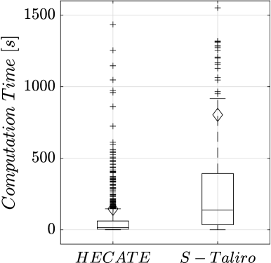
(a) Time (s)

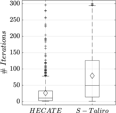
(b) Number of iterations

Figure 8: Time and number of iterations required by HECATE and S-Taliro to detect failure-revealing test cases. Diamonds depict the average.

Results. The box plots in Figure 8 report the time and number of iterations for HECATE and S-Taliro. HECATE and S-Taliro required on average 148.8s (min=3.7s, max=1503.6s, StdDev=369.2s). and 816.6s (min=2.1s, max=5255.6s, StdDev=1571.4s) to generate the failure-revealing test cases respectively. They performed on average 28.4 iterations (min=4.2, max=134.9, StdDev=31.2) and 99.9 iterations (min=3.4, max=276.0, StdDev=72.8). Therefore, HECATE is on average more efficient than S-Taliro. It required on average 667.8s ($816.6s-148.8s$) seconds less than S-Taliro. HECATE also required on average 71.5 ($99.9-28.4$) less iterations than S-Taliro. Table I (column RQ2) reports the average time in seconds and in parenthesis the average number of iterations for each model. Cells with green background refer to cases in which both the time and the number of iterations of HECATE is lower than the one of S-Taliro. Otherwise, cells have a red background. By considering each model separately, the average time and number of iterations required of HECATE are both lower than the one of S-Taliro for $\approx$81% of the models ($13$ out of $16$). Wilcoxon rank sum test ($\alpha$=$0.05$, p=$2.22\cdot 10^{-3}$) confirms that HECATE is more efficient than S-Taliro.

HECATE on average required 667.8s less seconds and 71.5 less iterations than S-Taliro to generate failure-revealing test cases. It was more efficient than S-Taliro for $\approx$81% of our benchmark models.

6.4 Usefulness (RQ3)

To answer RQ3, we considered a representative case study from the automotive domain. Our case study is a Simulink model of a hybrid-electric vehicle (HEV) developed by MathWorks for the EcoCAR Mobility Challenge [47]. The HEV model has $4641$ blocks, one input port, and one output port, and has simulation time set to $400$s. The HEV model converts electrical energy into mechanical energy. The model consists of different subsystems, including regenerative brake blending, battery management, power management, and software controller. These subsystems also use Simscape^®, Simscape^® Electrical^TM, and Simscape^® Driveline^TM blocks [59, 60, 61]. The controller is modeled as a Stateflow chart and adjusts the vehicle speed depending on the speed demand. The HEV comes with five driving scenarios, out of which we picked the scenario Urban Cycle 3 for our experiments.

Methodology. The speed demand of Urban Cycle 3 changes within the range $[0,90]$kph. We created a Test Sequence representing perturbations to be applied to the speed demand. It has four test steps, each describing the perturbation to be applied to the demanded speed within a $100$s time interval. We added four test parameters, one for each test step. We set their domain to $[0,4]$kph to ensure that our perturbations are lower than 5% of the maximum speed demand of the original driving scenario.

We designed a Test Assessment block that checks whether the delta speed, i.e., the absolute difference between the desired speed and the vehicle speed, is lower than a threshold value. For the original speed demand of Urban Cycle 3, the delta speed was always lower than $0.5$kph. We defined a Test Assessment block that tolerates a larger difference to account for the perturbations applied to the speed demand by the Test Sequence block. The Test Assessment block contains three test steps. The Test Sequence block starts applying perturbation at time instants $0$, $100$, $200$, and $300$. The first Test Assessment step is active in the time intervals $[0,1]$, $[100,101]$, $[200,201]$, $[300,301]$. It does not contain any verify or assert statements to enable the controller to adjust the vehicle speed to the changes in the speed demand. The second Test Assessment step is active within the time intervals $[1,10]$, $[101,110]$, $[201,210]$, $[301,310]$ and verifies whether the delta speed is lower than $1.5$kph. The third Test Assessment step is active within the time intervals $[10,100]$, $[110,200]$, $[210,300]$, $[310,400]$, and checks whether the delta speed is lower than the threshold value $1$kph. To summarize, after each perturbation to the speed demand, our Test Assessment provides $1$s and $10$s to enable the delta speed to become lower than the threshold values $1.5$kph and $1$kph.

For this evaluation, HECATE is set to run for a maximum $300$ iterations.

Results. HECATE returned a failure-revealing test case in $13$ iterations requiring $257$s ($\approx$4min). The values assigned to the four parameters of the Parameterized Test Sequence by the returned Test Sequence are $3.81$, $1.49$, $1.90$, and $3.66$. For this Test Sequence, the vehicle speed of the car ranges from $3.81$kph to $93.66$kph, while the delta speed ranges from $0$kph to $4$kph. The failure-revealing test case reveals the following problem. The controller needs more than one second to reduce the value of the delta speed below the $1.5$kph threshold for the perturbation applied to the vehicle speed by the first test step of the Test Sequence block. We analyzed the controller behavior to detect the problem. The controller has two modes: Start_mode, which is entered at the beginning of the simulation, and Normal_mode, which regulates the engine speed. The controller moves from Start_mode to Normal_mode when the engine speed exceeds a threshold of $800$rpm. The original speed demand for Urban Cycle 3 was $0$kph for the first $10$s. Our Test Sequence applied a small perturbation to this value for its first test step ($3.81$kph). Due to this perturbation, the engine speed takes more than $1$s to reach $800$rpm and to bring the controller to its Normal_mode. This leads to the violation of the condition specified by the test assessment, i.e., the controller needs more than one second to reduce the value of the delta speed below the $1.5$kph.

HECATE computed a failure-revealing test case for our automotive case study within $5$min by performing $13$ iterations. The failure-revealing test case shows that with a small perturbation in demanded speed, it takes the engine speed more than $1$s to reach $800$rpm and to bring the controller to its Normal_mode.

7 Discussion and Threats to Validity

This section reflects on our solution and results (Section 7.1) and elicits threats to validity (Section 7.2).

7.1 Reflections

Automatically generating failure-revealing test cases is a widely recognized software engineering problem [62, 63]. Providing support for Test Sequence and Test Assessment blocks is a significant problem since these blocks are widely used by practitioners [64, 65] and support standard compliance [66, 22]. There is no approach that solves this problem: HECATE is the first solution addressing the problem. Therefore, HECATE will significantly impact software engineering practices by enabling the automatic generation of test cases from manually specified Test Blocks.

Our solution is novel: search-based testing was never used with Test Sequence and Test Assessment blocks. The novelty concerns the development of a new testing solution addressing a relevant software engineering problem. We reused and adapted existing solutions to solve our problem, a recommended software engineering practice. We implemented our solution as a plugin for S-Taliro. The reuse of a mature tool (S-Taliro) for the development of HECATE makes our solution easily testable, maintainable, and extensible.

We answered RQ1 and RQ2 by comparing HECATE with S-Taliro. Assessing the effectiveness and efficiency of a solution by comparing it with a baseline is a sound technique widely used in the research literature (e.g., [6, 7]) also encouraged by international competitions (e.g., ARCH). Statistical tests confirmed the significance and soundness of our results. We answered RQ3 by assessing its applicability on a large case study. This is a sound technique largely used in the literature (e.g., [6]). Finally, RQ3 assesses whether HECATE can detect failure-revealing test cases for a large case study. Therefore, a comparison between HECATE and S-Taliro is not performed since it is not the objective of RQ3.

Our results are verifiable and transparent: our models, data, and tool are available for independent verification.

7.2 Threats to Validity

External Validity. The selection of the benchmark models for RQ1 and RQ2 and the case study model for RQ3 could threaten the external validity of our results. To mitigate this threat, we selected our benchmark models by including models extensively used in the literature (e.g., [38, 67, 44, 6, 17, 68]), from different domains (automotive, ML, electrical, and aerospace), from industry (AFC [44] is from Toyota, TUI, NNP, EU [45, 46] are from Lockheed Martin), and with a variable number of blocks (avg=$\approx 177.3$, min=$26$, max=$714$, StdDev=$\approx 182.9$). The number, size, and type of models considered in this work is consistent with similar works from this domain (e.g., [6]). We remark that (a) software companies do not usually share their Simulink models, and (b) we made our benchmark publicly available, enabling experiment replication. For RQ3, we selected a representative case study: it was developed by MathWorks for the EcoCAR Mobility Challenge [47].

The selection and definition of the Test Blocks and STL artifacts could threaten the external validity of our results since it influences the effectiveness and efficiency of HECATE and S-Taliro. To mitigate this threat we proceeded as follows. For RQ1 and RQ2, we considered Test Blocks and STL artifacts defined by (a) including models that already included STL artifacts and manually defining Test Blocks, (b) including models that already included Test Blocks and manually defining STL artifacts, (c) including models that did not include neither Test Blocks nor STL artifacts, and (d) testing the equivalence of the oracle generated from the STL specification and the Test Assessment blocks. For RQ3, we considered the model documentation for defining the Test Blocks.

Our results depend on Parameterized Test Sequence, its parameter domain, and Test Assessment blocks. Defining criteria to automatically define the Parameterized Test Sequence, its parameter domain, and Test Assessment blocks is out of the scope of this work and is left for future work.

Finally, the results for RQ1, RQ2, and RQ3 are likely to improve if the designers of Test Blocks are knowledgeable about the domain and have engineered the Simulink models.

Internal Validity. The selection of the values of the configuration parameters of HECATE and S-Taliro could threaten the internal validity of our results. To mitigate this threat, we selected the same values for the common configuration parameters of the two tools. Therefore, our configuration does not favor any of the tools.

8 Related Work

This section presents related testing frameworks that (a) support Simulink models, (b) support Test Blocks, and (c) start from manually specified test cases.

Simulink Models. There are two main categories of testing techniques for Simulink models: the ones that rely on simulation-based software testing (e.g., [29, 34, 6, 69, 68, 7, 70, 71, 72, 73, 74, 75, 15, 22, 76]), and the ones that need to access the internal structure of the models to generate test cases. The techniques from the first category do not support Test Blocks (see Section 1). HECATE extends these techniques by supporting Test Blocks and uses one of these techniques as baseline for our comparison (see Section 6). The techniques from the second category (e.g., Simulink Design Verifier [9] and Reactis[77]) need to access the internal structure of the models to generate test cases and usually attempt to satisfy some coverage metric. In addition, they do not support variable-step solvers or continuous time blocks, such as the Integrator, Derivative, or Transfer Function blocks. Therefore, we could not use these techniques as baseline for our experiment since they do not apply to a large set of models of our benchmark.

Simulink Test Blocks. A few approaches from the literature propose testing formalisms that are similar to Simulink Test Blocks [78, 79, 80, 81]. However, these works do not automatically generate test cases. Only a few approaches from the literature target Simulink Test Blocks (e.g., [82, 73, 83]). Unlike HECATE, these approaches (a) do not aim to generate a failure-revealing test case, but rather aim to satisfy coverage criteria [82, 73], or to identify performance-driven metamorphic relations [83]. Lastly, some approaches target formalisms named ‘test sequences’ [84, 85, 86, 87, 88] that are not related to Simulink and are significantly different from Simulink Test Sequences.

Manually Specified Test Cases. Several testing techniques generate new test cases from already existing, including manually defined test cases (see surveys [62, 63, 89, 90]). However, these approaches do not target Simulink models.

9 Conclusion

This work presented HECATE, a testing approach for Simulink models. Unlike existing approaches, HECATE uses the Test Sequence and Test Assessment blocks in Simulink Test to guide the search-based exploration. HECATE relies on Parameterized Test Sequences and on a procedure that compiles Test Assessment blocks into fitness functions. We implemented HECATE as a plugin for S-Taliro. We evaluated HECATE by comparing it with a baseline. Our results show that HECATE is more effective and efficient than our baseline. We also evaluated the applicability of HECATE on a representative automotive case study. HECATE successfully generated a failure-revealing test case for our case study.

Data Availability

A complete replication package containing our models, evaluation data, and tool is publicly available [57]. The EKF model is protected by an non-disclosure agreement and can not be shared publicly.

References

- [1] Math, “Simulink®,” Release R2022a, March 2022.
- [2] F. Elberzhager, A. Rosbach, and T. Bauer, “Analysis and testing of Matlab Simulink models: a systematic mapping study,” in International Workshop on Joining AcadeMiA and Industry Contributions to Testing Automation, 2013, pp. 29–34.
- [3] G. Liebel, N. Marko, M. Tichy, A. Leitner, and J. Hansson, “Model-based engineering in the embedded systems domain: an industrial survey on the state-of-practice,” Software and Systems Modeling, vol. 17, no. 1, pp. 91–113, 2018.
- [4] Y. Dajsuren, M. G. Van Den Brand, A. Serebrenik, and S. Roubtsov, “Simulink models are also software: Modularity assessment,” in International conference on Quality of software architectures. ACM, 2013, pp. 99–106.
- [5] A. Boll, F. Brokhausen, T. Amorim, T. Kehrer, and A. Vogelsang, “Characteristics, potentials, and limitations of open-source simulink projects for empirical research,” Software and Systems Modeling, vol. 20, no. 6, pp. 2111–2130, 2021.
- [6] C. Menghi, S. Nejati, L. Briand, and Y. I. Parache, “Approximation-refinement testing of compute-intensive cyber-physical models: An approach based on system identification,” in International Conference on Software Engineering. IEEE/ACM, 2020, pp. 372–384.
- [7] C. Menghi, S. Nejati, K. Gaaloul, and L. C. Briand, “Generating automated and online test oracles for simulink models with continuous and uncertain behaviors,” in European Software Engineering Conference and Symposium on the Foundations of Software Engineering (ESEC/FSE). ACM, 2019, pp. 27–38.
- [8] J. Kapinski, J. V. Deshmukh, X. Jin, H. Ito, and K. Butts, “Simulation-based approaches for verification of embedded control systems: An overview of traditional and advanced modeling, testing, and verification techniques,” IEEE Control Systems Magazine, vol. 36, no. 6, pp. 45–64, 2016.
- [9] MathWorks, “Simulink® Design VerifierTM,” Release R2022a, March 2022.
- [10] D. Giannakopoulou, T. Pressburger, A. Mavridou, and J. Schumann, “Generation of formal requirements from structured natural language,” in International working conference on requirements engineering: Foundation for software quality. Springer, 2020, pp. 19–35.
- [11] J. Kyriakidis and E. Vaz, “Informal fannal design verification: Experience from the industrial trenches,” in Digital Avionics Systems Conference (DASC). IEEE/AIAA, 2018, pp. 1–10.
- [12] S. Nejati, K. Gaaloul, C. Menghi, L. C. Briand, S. Foster, and D. Wolfe, “Evaluating model testing and model checking for finding requirements violations in simulink models,” in European Software Engineering Conference and Symposium on the Foundations of Software Engineering, ser. ESEC/FSE. ACM, 2019, p. 1015–1025.
- [13] “Prove Properties in a Model,” http://www.mathworks.com/help/sldv/ug/prove-properties-in-a-model.html#bq96vu4, 2022.
- [14] A. Arrieta Marcos, J. A. Agirre Bastegieta, and G. Sagardui Mendieta, “Seeding strategies for multi-objective test case selection: An application on simulation-based testing,” in Genetic and Evolutionary Computation Conference. ACM, 2020.
- [15] A. Schmidt, U. Durak, and T. Pawletta, “Model-based testing methodology using system entity structures for MATLAB/Simulink models,” Simulation, vol. 92, no. 8, pp. 729–746, 2016.
- [16] A. Rajhans, A. Mavrommati, P. J. Mosterman, and R. G. Valenti, “Specification and runtime verification of temporal assessments in simulink,” in International Conference on Runtime Verification. Springer, 2021, pp. 288–296.
- [17] G. Fainekos, B. Hoxha, and S. Sankaranarayanan, “Robustness of specifications and its applications to falsification, parameter mining, and runtime monitoring with s-taliro,” in International Conference on Runtime Verification. Springer, 2019, pp. 27–47.
- [18] A. Arrieta, J. A. Agirre, and G. Sagardui, “A tool for the automatic generation of test cases and oracles for simulation models based on functional requirements,” in International Conference on Software Testing, Verification and Validation Workshops. ACM/IEEE, 2020, pp. 1–5.
- [19] Z. Zhang, D. Lyu, P. Arcaini, L. Ma, I. Hasuo, and J. Zhao, “Effective hybrid system falsification using monte carlo tree search guided by qb-robustness,” in Computer Aided Verification. Springer, 2021, pp. 595–618.
- [20] ——, “On the effectiveness of signal rescaling in hybrid system falsification,” in NASA Formal Methods. Springer, 2021, pp. 392–399.
- [21] R. Matinnejad, S. Nejati, L. C. Briand, and T. Bruckmann, “Test generation and test prioritization for simulink models with dynamic behavior,” IEEE Transactions on Software Engineering, vol. 45, no. 9, pp. 919–944, 2018.
- [22] T. Schmidt, S. Jin, J. Rogalli, T. Rogier, H. Pohlheim, and I. Stürmer, “Efficient testing framework for simulink models with mtcd and automated test assessments in the context of iso 26262,” SAE International Journal of Passenger Cars-Electronic and Electrical Systems, vol. 7, no. 2014-01-0306, pp. 166–177, 2014.
- [23] “Reactis Testing Tools for Simulink and C Code,” http://www.reactive-systems.com/products.msp, 2022.
- [24] K. Juhnke, M. Tichy, and F. Houdek, “Challenges concerning test case specifications in automotive software testing: assessment of frequency and criticality,” Software Quality Journal, vol. 29, no. 1, pp. 39–100, 2021.
- [25] “ISO 26262,” http://www.iso.org/standard/43464.html, 2022.
- [26] MathWorks, “Simulink® TestTM,” Release R2022a, March 2022.
-
[27]
——, “Test Sequence,” Release R2022a.
https://www.mathworks.com/help/sltest/ref/testsequence.html, 2022. -
[28]
——, “Test Assessment,” Release R2022a.
https://www.mathworks.com/help/sltest/ref/testassessment.html, 2022. - [29] A. Donzé, “Breach, a toolbox for verification and parameter synthesis of hybrid systems,” in Computer Aided Verification. Springer, 2010, pp. 167–170.
- [30] M. Waga, “Falsification of cyber-physical systems with robustness-guided black-box checking,” in International Conference on Hybrid Systems: Computation and Control. ACM, 2020, pp. 11:1–11:13.
- [31] Y. Yamagata, S. Liu, T. Akazaki, Y. Duan, and J. Hao, “Falsification of cyber-physical systems using deep reinforcement learning,” IEEE Transactions on Software Engineering, vol. 47, no. 12, pp. 2823–2840, 2021.
- [32] G. Ernst, S. Sedwards, Z. Zhang, and I. Hasuo, “Fast falsification of hybrid systems using probabilistically adaptive input,” in International Conference on Quantitative Evaluation of Systems. Springer, 2018, pp. 165–181.
- [33] Z. Zhang, D. Lyu, P. Arcaini, L. Ma, I. Hasuo, and J. Zhao, “Effective hybrid system falsification using Monte Carlo Tree Search guided by QB-robustness,” in Computer Aided Verification. Springer, 2021, pp. 1–24.
- [34] Y. Annpureddy, C. Liu, G. Fainekos, and S. Sankaranarayanan, “S-TaLiRo: A Tool for Temporal Logic Falsification for Hybrid Systems,” in Tools and Algorithms for the Construction and Analysis of Systems. Springer, 2011, pp. 254–257.
- [35] O. Maler and D. Nickovic, “Monitoring temporal properties of continuous signals,” in Formal Techniques, Modelling and Analysis of Timed and Fault-Tolerant Systems. Springer, 2004, pp. 152–166.
- [36] C. Czepa, A. Amiri, E. Ntentos, and U. Zdun, “Modeling compliance specifications in linear temporal logic, event processing language and property specification patterns: a controlled experiment on understandability,” Software and Systems Modeling, vol. 18, no. 6, pp. 3331–3371, 2019.
- [37] C. Czepa and U. Zdun, “On the understandability of temporal properties formalized in linear temporal logic, property specification patterns and event processing language,” IEEE Transactions on Software Engineering, vol. 46, no. 1, pp. 100–112, 2018.
- [38] G. Ernst, P. Arcaini, I. Bennani, A. Chandratre, A. Donzé, G. Fainekos, G. Frehse, K. Gaaloul, J. Inoue, T. Khandait, L. Mathesen, C. Menghi, G. Pedrielli, M. Pouzet, M. Waga, S. Yaghoubi, Y. Yamagata, and Z. Zhang, “ARCH-COMP category report: Falsification with validation of results,” in Workshop on Applied Verification of Continuous and Hybrid Systems, vol. 80. EasyChair, 2021, pp. 133–152.
- [39] M. Ayesh, N. Mehan, E. Dhanraj, A. El-Rahwan, S. E. Opalka, T. Fan, A. Hamilton, A. M. Jacob, R. A. Sundarrajan, B. Widjaja, and C. Menghi, “Two simulink models with requirements for a simple controller of a pacemaker device,” in Proceedings of 9th International Workshop on Applied Verification of Continuous and Hybrid Systems (ARCH22), ser. EPiC Series in Computing, vol. 90. EasyChair, 2022, pp. 18–25.
- [40] “Use Test Sequence Scenarios in the Test Sequence Editor and Test Manager,” http://www.mathworks.com/help/sltest/ug/define-test-sequence-scenarios-in-test-sequence-editor.html, 2022.
- [41] “Assess a Model by Using When Decomposition,” http://www.mathworks.com/help/sltest/ug/using-when-decomposition-to-write-tests.html, 2022.
- [42] “Assess the Damping Ratio of a Flutter Suppression System,” http://www.mathworks.com/help/sltest/ug/assess-damping-ratio-of-flutter-suppression-system.html, 2022.
- [43] “Test Traffic Light Control by Using Logical and Temporal Assessments,” http://www.mathworks.com/help/sltest/ug/test-traffic-light-using-logical-and-temporal-assessments.html, 2022.
- [44] X. Jin, J. V. Deshmukh, J. Kapinski, K. Ueda, and K. Butts, “Powertrain control verification benchmark,” in International conference on Hybrid systems: computation and control. ACM, 2014, pp. 253–262.
- [45] A. Mavridou, H. Bourbouh, D. Giannakopoulou, T. Pressburger, M. Hejase, P.-L. Garoche, and J. Schumann, “The ten lockheed martin cyber-physical challenges: formalized, analyzed, and explained,” in International Requirements Engineering Conference. IEEE, 2020, pp. 300–310.
- [46] C. Elliott, “On example models and challenges ahead for the evaluation of complex cyber-physical systems with state of the art formal methods V&V, Lockheed Martin Skunk Works,” in Safe & Secure Systems and Software Symposium, 2015, pp. 9–11.
- [47] “The EcoCAR Mobility Challenge ,” http://www.mathworks.com/ academia/student-competitions/ecocar.html, 2022.
- [48] “Test Sequence and Assessment Syntax,” https://www.mathworks.com /help/sltest/ug/syntax-for-test-sequences-and-assessments.html, 2022.
- [49] MathWorks, “Stateflow®,” Release R2022a, March 2022.
- [50] G. E. Fainekos and G. J. Pappas, “Robustness of temporal logic specifications,” in Formal Approaches to Software Testing and Runtime Verification. Springer, 2006, pp. 178–192.
- [51] H. Abbas, B. Hoxha, G. Fainekos, and K. Ueda, “Robustness-guided temporal logic testing and verification for stochastic cyber-physical systems,” in International Conference on Cyber Technology in Automation, Control and Intelligent. IEEE, 2014, pp. 1–6.
- [52] T. Nghiem, S. Sankaranarayanan, G. Fainekos, F. Ivancić, A. Gupta, and G. J. Pappas, “Monte-carlo techniques for falsification of temporal properties of non-linear hybrid systems,” in International conference on Hybrid systems: computation and control. ACM, 2010, pp. 211–220.
- [53] H. Abbas, A. Winn, G. Fainekos, and A. A. Julius, “Functional gradient descent method for metric temporal logic specifications,” in American Control Conference. IEEE, 2014, pp. 2312–2317.
- [54] “Simulate a Simulink model,” http://www.mathworks.com/help/ simulink/ slref/sim.html, 2022.
- [55] “International Competition on Verifying Continuous and Hybrid Systems (ARCH),” http://cps-vo.org/group/ARCH/FriendlyCompetition, 2022.
- [56] C. E. Tuncali, B. Hoxha, G. Ding, G. Fainekos, and S. Sankaranarayanan, “Experience report: Application of falsification methods on the uxas system,” in NASA Formal Methods. Springer, 2018, pp. 452–459.
- [57] “HECATE,” https://github.com/Hecate-SBST/Hecate, 2022.
- [58] J. Duque, P. J. Kollmeyer, M. Naguib, and A. Emadi, “Battery dual extended kalman filter state of charge and health estimation strategy for traction applications,” in Transportation Electrification Conference & Expo. IEEE, 2022, pp. 975–980.
- [59] MathWorks, “Simscape®,” Release R2022a, March 2022.
- [60] ——, “Simscape® ElectricalTM,” Release R2022a, March 2022.
- [61] ——, “Simscape® DrivelineTM,” Release R2022a, March 2022.
- [62] M. Papadakis, M. Kintis, J. Zhang, Y. Jia, Y. Le Traon, and M. Harman, “Mutation testing advances: an analysis and survey,” in Advances in Computers. Elsevier, 2019, vol. 112, pp. 275–378.
- [63] S. Ali, L. C. Briand, H. Hemmati, and R. K. Panesar-Walawege, “A systematic review of the application and empirical investigation of search-based test case generation,” IEEE Transactions on Software Engineering, vol. 36, no. 6, pp. 742–762, 2010.
- [64] S. W. Dalton, F. Wagner, A. Bergmann, and B. Bock, “Using MATLAB V&V-Toolbox for Target-Specific Model-Based Design,” in International Conference on Engineering Science and Innovative Technology. IEEE, 2018, pp. 1–5.
- [65] F. Wagner, S. W. Dalton, and A. Bergmann, “Benefits and drawbacks of target specific model-based testing,” in International Conference on Research and Education in Mechatronics. IEEE, 2017, pp. 1–5.
- [66] D. Hoadley, “Using Model-Based Design in an IEC 62304-Compliant Software Development Process.” in MBEES, 2010, pp. 129–131.
- [67] A. Fehnker and F. Ivančić, “Benchmarks for hybrid systems verification,” in International Workshop on Hybrid Systems: Computation and Control. Springer, 2004, pp. 326–341.
- [68] A. Donzé and O. Maler, “Robust satisfaction of temporal logic over real-valued signals,” in Formal Modeling and Analysis of Timed Systems. Springer, 2010, pp. 92–106.
- [69] M. Waga, “Falsification of cyber-physical systems with robustness-guided black-box checking,” in International Conference on Hybrid Systems: Computation and Control. ACM, 2020.
- [70] R. Matinnejad, S. Nejati, L. C. Briand, and T. Bruckmann, “Automated test suite generation for time-continuous Simulink models,” in International Conference on Software Engineering. ACM/IEEE, 2016, pp. 595–606.
- [71] ——, “Automated test suite generation for time-continuous Simulink models,” in International Conference on Software Engineering. ACM, 2016, pp. 595–606.
- [72] R. Matinnejad, S. Nejati, L. Briand, and T. Brcukmann, “MiL Testing of Highly Configurable Continuous Controllers: Scalable Search Using Surrogate Models,” in International Conference on Automated Software Engineering. ACM/IEEE, 2014, p. 163–174.
- [73] P. Peranandam, S. Raviram, M. Satpathy, A. Yeolekar, A. Gadkari, and S. Ramesh, “An integrated test generation tool for enhanced coverage of simulink/stateflow models,” in Design, Automation & Test in Europe Conference & Exhibition. IEEE, 2012, pp. 308–311.
- [74] F. Lindlar, A. Windisch, and J. Wegener, “Integrating model-based testing with evolutionary functional testing,” in International conference on software testing, verification, and validation workshops. IEEE, 2010, pp. 163–172.
- [75] A. Arrieta, U. Markiegi, and L. Etxeberria, “Towards Mutation Testing of Configurable Simulink Models: a Product Line Engineering Perspective,” Jornadas de Ingeniera del So ware y Bases de Datos, 2017.
- [76] I. Pill, I. Rubil, F. Wotawa, and M. Nica, “Simultate: A toolset for fault injection and mutation testing of simulink models,” in International Conference on Software Testing, Verification and Validation Workshops. IEEE, 2016, pp. 168–173.
- [77] “Reactis,” http://www.reactive-systems.com/doc/reactis-for-simulink/, 2022.
- [78] E. Bringmann and A. Krämer, “Systematic testing of the continuous behavior of automotive systems,” in Workshop on Software engineering for automotive systems. ACM, 2006, pp. 13–20.
- [79] E. Bringmann, “Testing the continuous behavior of embedded systems,” in Workshop on System Testing and Validation, 2007.
- [80] P. R. Srivastava et al., “Automatic test sequence generation for state transition testing via ant colony optimization,” in Evolutionary Computation and Optimization Algorithms in Software Engineering: Applications and Techniques. IGI Global, 2010, pp. 161–183.
- [81] P. R. Srivastava and K. Baby, “Automated software testing using metahurestic technique based on an ant colony optimization,” in Symposium on electronic system design. IEEE, 2010, pp. 235–240.
- [82] J. Ferrer, P. M. Kruse, F. Chicano, and E. Alba, “Search based algorithms for test sequence generation in functional testing,” Information and Software Technology, vol. 58, pp. 419–432, 2015.
- [83] J. Ayerdi, P. Valle, S. Segura, A. Arrieta, G. Sagardui, and M. Arratibel, “Performance-driven metamorphic testing of cyber-physical systems,” IEEE Transactions on Reliability, 2022.
- [84] A. Bombarda and A. Gargantini, “An automata-based generation method for combinatorial sequence testing of finite state machines,” in International conference on software testing, verification and validation workshops. IEEE, 2020, pp. 157–166.
- [85] S. Hallé and R. Khoury, “SealTest: a simple library for test sequence generation,” in International Symposium on Software Testing and Analysis. ACM SIGSOFT, 2017, pp. 392–395.
- [86] Y. Sheng, S. Jiang, and C. Wei, “Constructing test suites for real-time embedded systems under input timing constraints,” IEEE Access, vol. 7, pp. 20 920–20 937, 2019.
- [87] S. Hallé and R. Khoury, “Test sequence generation with cayley graphs,” in International Conference on Software Testing, Verification and Validation Workshops. IEEE, 2021, pp. 182–191.
- [88] Y. Sheng, C. Sun, S. Jiang, and C. Wei, “Extended covering arrays for sequence coverage,” Symmetry, vol. 10, no. 5, p. 146, 2018.
- [89] M. Khari and P. Kumar, “An extensive evaluation of search-based software testing: a review,” Soft computing, vol. 23, no. 6, pp. 1933–1946, 2019.
- [90] M. Harman, Y. Jia, and Y. Zhang, “Achievements, open problems and challenges for search based software testing,” in Conference on Software Testing, Verification and Validation. IEEE, 2015, pp. 1–12.