Analysis of a $\operatorname{sinc}$-Galerkin Method for the Fractional Laplacian

Abstract.

We provide the convergence analysis for a $\operatorname{sinc}$-Galerkin method to solve the fractional Dirichlet problem. This can be understood as a follow-up of [5], where the authors presented a $\operatorname{sinc}$-function based method to solve fractional PDEs. While the original method was formulated as a collocation method, we show that the same method can be interpreted as a nonconforming Galerkin method, giving access to abstract error estimates. Optimal order of convergence is shown without any unrealistic regularity assumptions on the solution.

1. Introduction

Motivated by a number of applications, we aim to solve the fractional Dirichlet problem, i.e., find $u$ in an appropriate space such that

$$(-\Delta)^{s}u=f\text{ in }\Omega,\quad u\equiv 0\text{ in }\mathbb{R}^{d}\setminus\Omega.$$ (1.1)

We are dealing with the integral definition of the fractional Laplacian which – in terms of the Fourier transformation – can be defined as

$$\operatorname{\mathcal{F}}\left((-\Delta)^{s}u\right)(\omega)=|\omega|^{2s}\hat{u}(\omega),$$ (1.2)

where $\hat{u}(\omega)=\left(\operatorname{\mathcal{F}}u\right)(\omega)$ is the Fourier transformation of $u$. If defined on the whole ${\mathbb{R}^{d}}$, at least ten different, but equivalent definitions of the fractional Laplacian exist [27]. One of the definitions that we want to mention here is the integral definition which reads [14]

$$(-\Delta)^{s}u=C(d,s)\text{P.V.}\int_{\mathbb{R}^{d}}\frac{u(x)-u(y)}{\left|{x-y}\right|^{d+2s}}\mathop{\mathrm{d}y}$$ (1.3)

and exposes the nonlocal character of the fractional Laplacian: to evaluate $(-\Delta)^{s}u(x)$ at one point $x\in{\mathbb{R}^{d}}$, a singular integral over the whole ${\mathbb{R}^{d}}$ has to be evaluated. This makes numerical approximations of eq. 1.1 challenging. A proof for the equivalence of eq. 1.2 and eq. 1.3, as well as the exact value of the constant $C(d,s)$, can be found – among others – in [14].

Various approaches to solve such problems have been proposed in the last years. The article [2], provides the analysis and implementation of a finite element Galerkin method for the fractional ($s$)-Poisson problem on Lipschitz domains. For $\mathbb{P}_{1}$-finite elements, this leads to a conforming finite element method assuming $s\in(0,1)$. Further studies on finite element methods for the fractional Dirichlet problem can be found for example in [3, 4, 7, 8]. Some further examples of approximations of nonlocal problems can be found in [17, 26].

Finite difference methods have been proposed in, e.g., [25]. Such finite-difference formulations of fractional PDE on Cartesian grids lead to linear systems with matrices that can be efficiently applied to vectors using fast Fourier transformation (FFT) based algorithms. Examples of algorithms of this type can be found in [28] or in [16] and, of course, our aforementioned work. However, the analysis for such algorithms typically needs strong regularity assumptions or is limited to rectangular domains.

In [5], we proposed a collocation method to solve eq. 1.1 where we used a $\operatorname{sinc}$-basis to solve the equation pointwise on a grid. More concretely, we find a function

$$u_{h}(x)=\sum\limits_{k\in{\mathbb{Z}^{d}}}u_{k}\varphi^{N}_{k}(x),\quad u_{k}\in\mathbb{R}$$ (1.4)

satisfying

$$(-\Delta)^{s}u_{h}(x_{k}) =f_{k} \text{ if }x_{k}=hk\in\Omega$$ (1.5)

$$u_{h}(x_{k}) =0 \text{ if }x_{k}=hk\not\in\Omega\,.$$

The functions $\varphi^{N}_{k}(x)$ are $\operatorname{sinc}$-functions which we scale by a parameter $N$ and shift by $k$ gridpoints. The natural number $N>0$ is the number of grid points we use in each spatial direction and $h\coloneqq 1/N$ is the grid spacing. We will interchangeably use $N$ or $h=1/N$ depending on the context. The equation $u_{h}(x_{k})=0$ if $x_{k}\not\in\Omega$ is equivalent to $u_{k}=0$ if $x_{k}\not\in\Omega$ as the basis functions fulfill the Kronecker-delta property $\varphi^{N}_{k}(x_{j})=\delta_{k,j}$. We detail this in section 2.1, as well as we briefly recall the $\operatorname{sinc}$-collocation method and its efficient implementation we presented in the aforementioned paper.

Our approach to solve the fractional Dirichlet problem, formulated as a collocation method, can be viewed also as a finite difference method. For the case $d=1$, this has been established in [25]. As we pointed out in [5], our approach for solving eq. 1.1 in more than one dimension can be seen as a multi-dimensional generalization of this. Other works in this direction can be found e.g. in the work [24] by the same authors as [25] where a finite difference scheme based on quadrature of the singular integrals is defined; in [21] where a similar technique as in [24] is used to obtain a discretization of the operator on unstructured grids.

Another approach that is related to ours is [22]. They define a discrete convolution operator whose coefficients are obtained via cubature in Fourier space. This approach can be extended to non-rectangular domains using the fictious domain method.

As we detail in the following, our method can also be seen as a Galerkin method using a $\operatorname{sinc}$-basis consisting of $C^{\infty}$-functions with unbounded support. In stark contrast to, e.g., [2], this leads to a nonconforming Galerkin method. Nevertheless, similarly to [2], no additional regularity of the solution is assumed other than what has been shown in the literature for such problems.

In our aforementioned work, we could demonstrate the effectiveness of our method on a benchmark problem where $\Omega$ is a ball in ${\mathbb{R}^{d}}$ and $f\equiv 1$ in $\Omega$. We also used it to solve problems with high spatial resolution, with a minimal computational expense. Indeed, our method has quasi-linear complexity, which is also visible in our computational results. For example, solving eq. 1.1 with $s=1/2$ and about $6\cdot 10^{6}$ grid points in $\mathbb{R}^{3}$ takes approximately $12$ minutes wall clock time on a standard office work station. This includes the setup of the operator (approx. $10$ minutes) and the solve of the system (approx. $2$ minutes), which we improved in comparison to the implementation presented in [5], with the use of a simple periodic fractional Laplacian as a preconditioner.

However, a numerical analysis of the method presented in [5] was still pending. This paper aims to close this gap. We want to emphasize at this point that all the implementation details as well as the pseudo-code that we already provided in [5] may remain unchanged. We show quasi-optimal rates of convergence in terms of the energy norm which are in agreement with the results that we obtained in numerical experiments. Briefly, our main result is that for $f\in C^{\frac{1}{2}}(\overline{\Omega})$ and under suitable assumptions on the domain $\Omega$, the solution $u_{h}$ we obtain via eq. 1.5, taking $f_{k}=f(x_{k})$ for $x_{k}\in\Omega$, fulfills the estimate

$$\left\|{u-u_{h}}\right\|_{H^{s}({\mathbb{R}^{d}})}\leq C(d,s,\Omega)\,\left\|{f}\right\|_{C^{\frac{1}{2}}(\overline{\Omega})}\,\left|{\log{h}}\right|h^{1/2}$$ (1.6)

where $u$ is the exact solution to the problem and $h$ is the grid spacing. We show this in theorem 5.2. In our analysis, we need to assume that there exists a Hölder continuous extension of $f$ to a domain that is slightly larger than $\Omega$. Thus, we require $f\in C^{\beta}(\overline{\Omega})$ for an appropriate $\beta$. When $\beta\geq\frac{1}{2}$, the above result applies directly as then the result of an extension-and-mollification procedure applied to $f$ agrees sufficiently well with the original function. In cases where $f$ has more limited regularity, we need to replace the discrete right-hand side $f_{k}$ by an evaluation of a suitable extended-and-mollified right hand side. For this approximation, we show that eq. 1.6 holds in theorem 5.1. In our proofs, we make substantial use of the regularity of the solutions shown in [2, 11, 30]. The only additional assumptions we have to make concern the domain and the right-hand side. We assume that one can slightly enlarge the domain and, when considering eq. 1.1 on the enlarged domain, have similar regularity of solutions as for the problem on the original domain. Details are given in section 4.3.

To establish the rates of convergence, we show how the collocation method can be equivalently written as a Galerkin method. As the resulting method is nonconforming, we must apply a Strang type lemma, see e.g. [12], and bound the resulting error terms appropriately. This reduces to showing that the chosen $\operatorname{sinc}$-basis can approximate the elements of the fractional Sobolev space $\widetilde{H}^{s}(\Omega)$ as well as the elements of its dual.

The remainder of this paper is structured as follows. In section 2, we summarize results of related work that this article is based on. This includes a brief overview of the $\operatorname{sinc}$-collocation method we presented in [5] as well as the weak formulation of eq. 1.1 and results from regularity theory that we need.

In section 3, we provide the formulation of the $\operatorname{sinc}$-Galerkin method. This includes the definitions of the grid-dependent discrete spaces as well as some properties of them, such as for example a Poincaré inequality, and inverse-estimate type result and properties of the norms on the spaces. Further, we present the abstract error estimate that we use here.

In section 4, we compute the approximation errors in the discrete spaces which, using the abstract error estimate, immediately yields the optimal rate of convergence for our numerical method in fractional Sobolev norms. For this, we must make some additional assumptions on the regularity of the domain.

Finally, section 5, contains our main theorems.

2. Notation and Preliminary Results

We briefly recapitulate known results that will be useful for the present work. In particular, we discuss the $\operatorname{sinc}$-basis collocation method, as well as regularity theory.

2.1. The $\operatorname{sinc}$-collocation method

In [5], we proposed to approximate eq. 1.1 in a $\operatorname{sinc}$-basis. Using the $d$-fold Cartesian product of $\operatorname{sinc}$-functions, we defined a basis function

$$\varphi(x)\coloneqq\prod\limits_{i=1}^{d}\operatorname{sinc}(x_{i}),\quad\operatorname{sinc}(x)\coloneqq\frac{\sin(\pi x)}{\pi x},\quad x=(x_{1}\cdots x_{d})^{T}\in{\mathbb{R}^{d}},$$ (2.1)

and its dilated and shifted versions,

$$\varphi^{N}_{k}(x)=\varphi(Nx-k),\quad k=(k_{1}\cdots k_{d})^{T}\in\mathbb{Z}^{d},$$ (2.2)

which span our discrete space. Throughout this work, we use the conventions

$$\operatorname{\mathcal{F}}u(\omega)=(2\pi)^{-d}\int_{\mathbb{R}^{d}}u(x)\mathrm{e}^{-i\omega x}\mathop{\mathrm{d}x},\qquad\operatorname{\mathcal{F}^{-1}}\hat{u}(x)=\int_{\mathbb{R}^{d}}\hat{u}(\omega)\mathrm{e}^{\mathrm{i}\omega x}\mbox{d}\omega.$$ (2.3)

For this specific scaling of the Fourier transformation, we have the Plancherel identity

$$(v,w)_{L^{2}({\mathbb{R}^{d}})}=(2\pi)^{d}(\hat{v},\hat{w})_{L^{2}({\mathbb{R}^{d}})}.$$ (2.4)

A well-known result (see, e.g., [31]) is that

$$\operatorname{sinc}(x)=\frac{1}{2\pi}\int_{[-\pi,\pi]}\mathrm{e}^{\mathrm{i}\omega x}\mathop{\mathrm{d}\omega}=\frac{1}{2\pi}\operatorname{\mathcal{F}^{-1}}\chi_{[-\pi,\pi]}(\omega),$$ (2.5)

so that $\operatorname{\mathcal{F}}\varphi(\omega)=\frac{1}{(2\pi)^{d}}\chi_{[-\pi,\pi]^{d}}(\omega)$ and, using the Fourier shift and scaling theorems,

$$\widehat{\varphi^{N}_{k}}(\omega)=N^{-d}\mathrm{e}^{-\mathrm{i}\omega k/N}\hat{\varphi}(\omega/N)=(2N\pi)^{-d}\mathrm{e}^{-\mathrm{i}\omega k/N}\chi_{D_{N}}(\omega),\quad D_{N}\coloneqq[-N\pi,N\pi]^{d}.$$ (2.6)

In order to solve eq. 1.1, we proposed in [5] to solve the problem pointwise on the grid $h\mathbb{Z}^{d}$, $h\coloneqq 1/N$, in the sense of a collocation method. As presented in eq. 1.5 this formulation leads to the linear system

$$S_{\Omega}\Phi^{N}S_{\Omega}^{T}\vec{u}=\vec{f},$$ (2.7)

and we provided efficient strategies to assemble the system matrix $\Phi^{N}$ and to solve the resulting system. In eq. 2.7, $\vec{u}=(u_{k})$ is the sought-after coefficient vector of the solution $u_{h}$ and $\vec{f}=(f_{k})_{k/N\in\Omega}$ is the discrete right-hand side which we obtained as pointwise evaluations of $f$ within $\Omega$ for the numerical experiments in [5]. $S_{\Omega}$ is a linear operator which leaves the coefficients within the domain unchanged and sets the others to zero, thus restricting the domain of computation. When we numerically solve this system, this approach is the projected conjugate gradient method, alternatively our method can be viewed as a constrained quadratic optimization problem which we solve using a null-space approach.

The application of the system matrix to a coefficient vector $\vec{u}$ is essentially the discrete convolution with the fractional Laplacian of the basis function $\varphi$ above, namely

$$(\Phi^{N}\vec{u})_{j}=\sum\limits_{k\in\{0\ldots N-1\}^{d}}u_{k}\Phi^{N}(j-k),\quad\Phi^{N}(j-k)=N^{2s}(-\Delta)^{s}\varphi(j-k).$$ (2.8)

This convolution can be computed efficiently using the discrete Fourier transformation, leading to a numerical complexity of $\mathcal{O}(N^{d}\cdot\log(N^{d}))$.

2.2. Weak formulation of the boundary value problem

The weak formulation of eq. 1.1 reads as follows [30, 2, 8]. Find $u\in\mathbb{V}$ such that

$$a(u,v)=F(v)\quad\text{for all $v\in\mathbb{V}$}$$ (2.9)

where $\mathbb{V}$ is the space

$$\mathbb{V}\coloneqq\widetilde{H}^{s}(\Omega)=\{v\in H^{s}({\mathbb{R}^{d}})\,|\,v=0\ {\rm in}\ \mathbb{R}^{d}\setminus\Omega\}$$ (2.10)

and $H^{s}({\mathbb{R}^{d}})$ is a fractional Sobolev space [14]. The bilinear form $a:\mathbb{V}\times\mathbb{V}\longrightarrow\mathbb{R}$ reads

$$a(u,v)=\int\limits_{\mathbb{R}^{d}}(-\Delta)^{\frac{s}{2}}u\cdot(-\Delta)^{\frac{s}{2}}v\mathop{\mathrm{d}x},$$ (2.11)

and the linear form $F(\cdot)$ is given by

$$F(v)=\int_{\Omega}fv\mathop{\mathrm{d}x}$$ (2.12)

for $f\in L^{2}(\Omega)$. Using the Plancherel identity, the bilinear form can be evaluated in the Fourier domain, which yields

$$a(u,v)=(2\pi)^{d}\int\limits_{\mathbb{R}^{d}}|\omega|^{2s}\hat{u}{\hat{v}}^{*}\mathop{\mathrm{d}\omega}$$ (2.13)

where the asterisk denotes the complex conjugate. The fractional Sobolev seminorm for $u\in H^{s}({\mathbb{R}^{d}})$ is defined as

$$\left|{u}\right|_{H^{s}(\mathbb{R}^{d})}\coloneqq a(u,u)^{1/2}=\left((2\pi)^{d/2}\int_{\mathbb{R}^{d}}\left|{\omega}\right|^{2s}\left|{\hat{u}}\right|^{2}\right)^{1/2}.$$ (2.14)

Given a suitable finite dimensional subspace $V_{h}\subset\mathbb{V}$, an abstract Galerkin method can be formulated as follows. Find $u_{h}\in V_{h}$ such that

$$a(u_{h},v_{h})=F(v_{h})\quad\text{for all $v_{h}\in V_{h}$}.$$ (2.15)

This Galerkin formulation can be used as to derive a finite element method (see, e.g., [2]); a non-conforming version thereof also forms the basis of our convergence analysis.

2.3. Summary of results from the literature

For our analysis, we require certain regularity and decay properties of solutions to eq. 1.1 and some mathematical key tools. In particular, we require [30, Lemma 2.7], which we repeat here for the reader’s convenience.

Theorem 2.1 (Lemma 2.7 in [30]).

Let $\Omega$ be a bounded domain satisfying the exterior ball condition and let $f\in L^{\infty}(\Omega)$. Let $u$ be the solution of eq. 1.1. Then,

$$\left|{u(x)}\right|\leq C\left\|{f}\right\|_{L^{\infty}(\Omega)}\operatorname{dist}(x,\Omega^{c})^{s}$$ (2.16)

where $C=C(\Omega,s)$ is a constant depending only on $\Omega$ and $s$.

Acosta and Borthagaray [11, 2] use global Hölder regularity of solutions (also proved in [30]) to derive estimates for $u$ in fractional Sobolev norms. Again, we repeat the result here for the reader’s convenience.

Theorem 2.2 (Proposition 2.4 in [11]).

Let $\Omega$ be a Lipschitz domain satisfying the exterior ball condition and consider $\beta=1/2-s$ if $s<1/2$ or $\beta>0$ if $s\geq 1/2$. Then, if $f\in C^{\beta}(\Omega)$, the solution $u$ of eq. 1.1 belongs to $\widetilde{H}^{s+1/2-\theta}(\Omega)$ with

$$\left\|{u}\right\|_{\widetilde{H}^{s+1/2-\theta}(\Omega)}\leq\frac{C(\Omega,s,d)}{\theta}\left\|{f}\right\|_{C^{\beta}(\Omega)}$$ (2.17)

for any $\theta>0$.

If $\Omega$ is smooth, no Hölder-regularity of $f$ is needed in order to have Sobolev-regularity of the solution $u$. In fact, in that case, we have the following theorem.

Theorem 2.3 (Proposition 2.7 in [11]).

Let $\Omega$ be a smooth domain, $f\in H^{r}(\Omega)$ for $r\geq-s$ and $u\in\widetilde{H}^{s}(\Omega)$ be the solution of the Dirichlet problem eq. 1.1. Then, the following regularity estimate holds

$$\left|{u}\right|_{H^{s+\alpha}({\mathbb{R}^{d}})}\leq C(d,\alpha)\left\|{f}\right\|_{H^{r}(\Omega)}.$$

Here, $\alpha=s+r$ if $s+r<\frac{1}{2}$ and $\alpha=\frac{1}{2}-\theta$ if $s+r\geq\frac{1}{2}$, with $\theta>0$ arbitrarly small.

Remark 2.1.

In the following, approximation errors depend on the decay of the solution to the boundary in the sense of Theorem 2.1 and on the $\left|{\,\cdot\,}\right|_{H^{t}({\mathbb{R}^{d}})}$-seminorm of the solution $u$ for some $t>s$ in the sense of Theorems 2.2 and 2.3. To simplify the statements, we write

$$u(x)\leq C_{\text{Bndry.}}(\Omega,f,s)\operatorname{dist}(x,\Omega^{c})^{s}$$

and

$$\left\|{u}\right\|_{H^{t}({\mathbb{R}^{d}})}\leq C_{\text{Sob.}}(\Omega,f,s)$$

for the solution $u$ to the exterior value problem on a suitable domain $\Omega$ and a given right-hand side $f$. The constant $C_{\text{Sob.}}(\Omega,f,s)$ has to be chosen appropriately, depending on the given domain and right-hand side, in the sense of Theorems 2.2 and 2.3. We note that other results regarding Sobolev regularity, as, e.g., in [1], may be used to obtain our convegence rates as well. This could lead to different requirements on the domain regularity.

Another key ingredient for our proofs is the Poisson summation formula (PSF) that can be stated as follows

Theorem 2.4 (Poisson summation formula).

Suppose that $u,\hat{u}\in L^{1}({\mathbb{R}^{d}})$ satisfy

$$\left|{u(x)}\right|+\left|{\hat{u}(x)}\right|\leq C\left(1+\left|{x}\right|\right)^{-d-\delta}$$ (2.18)

for some $C,\delta>0$. Then $u$ and $\hat{u}$ are both continuous and for all $x\in{\mathbb{R}^{d}}$ we have

$$\frac{1}{(2N\pi)^{d}}\sum\limits_{k\in{\mathbb{Z}^{d}}}u(k/N)\mathrm{e}^{-\mathrm{i}k/N}=\sum\limits_{k\in{\mathbb{Z}^{d}}}\hat{u}(2N\pi k+\omega)$$ (2.19)

For a proof, see Theorem 3.1.17 in [20] after appropriately rescaling to match the conventions of the Fourier transformations used there and exchanging the roles of $\operatorname{\mathcal{F}}$ and $\operatorname{\mathcal{F}^{-1}}$ or [29].

3. Formulation of the $\operatorname{sinc}$-Galerkin method

We now formulate a Galerkin method on the space of $\operatorname{sinc}$-functions, which yields the same solutions as the $\operatorname{sinc}$-collocation method introduced earlier.

3.1. Discrete Function Spaces

As a first discrete space, we define

$$\mathbb{V}_{h}({\mathbb{R}^{d}})=\left\{v_{h}\Big{|}v_{h}=\sum\limits_{k\in{\mathbb{Z}^{d}}}v_{k}\varphi^{N}_{k}(x),\,k\in{\mathbb{Z}^{d}}\right\}\cap H^{s}({\mathbb{R}^{d}})$$ (3.1)

using scaled and shifted $\operatorname{sinc}$-functions $\varphi^{N}_{k}(x)$ as our basis. To actually implement the method, we need a finite-dimensional subspace of $\mathbb{V}_{h}({\mathbb{R}^{d}})$. We take

$$\mathbb{V}_{h}(\Omega)=\left\{v_{h}=\sum\limits_{k\in\Omega_{h}}v_{k}\varphi^{N}_{k}(x)\right\},\quad\Omega_{h}=\left\{k\in{\mathbb{Z}^{d}}\text{ s.t. }k/N\in\Omega\right\}.$$ (3.2)

Denoting grid points by $x_{k}\coloneqq k/N$, we mention that for $k,l\in{\mathbb{Z}^{d}}$ we have $\varphi^{N}_{k}(x_{k})=1$ and $\varphi^{N}_{k}(x_{l})=0$ if $k\neq l$. We implicitly extend functions $v\in\mathbb{V}_{h}(\Omega)$ to functions in $\mathbb{V}_{h}({\mathbb{R}^{d}})$ by setting the coefficients in $h{\mathbb{Z}^{d}}\setminus\Omega_{h}$ to $0$.

Complementary to the extension, we define a discrete restriction operator ${\cdot}\big{|}_{\Omega_{h}}:\mathbb{V}_{h}({\mathbb{R}^{d}})\rightarrow\mathbb{V}_{h}(\Omega)$ via

$${v_{h}}\big{|}_{\Omega_{h}}(x)=\sum\limits_{k\in\Omega_{h}}v_{k}\varphi^{N}_{k}(x).$$ (3.3)

We emphasize that the restriction operator ${\cdot}\big{|}_{\Omega_{h}}$ does not actually restrict the support of the continuous function $v_{h}$ to $\Omega$, but only the sum of the coefficients to the coefficients with index $k\in\Omega_{h}$.

3.1.1. Orthogonality properties of the discrete spaces

We first note that the basis functions $\varphi^{N}_{k},k\in{\mathbb{Z}^{d}}$ form an $L^{2}$-orthogonal system. Indeed, we have, for $k,j\in{\mathbb{Z}^{d}}$,

$$\left(\varphi^{N}_{k},\varphi^{N}_{j}\right)_{L^{2}({\mathbb{R}^{d}})} =(2\pi)^{d}\int_{{\mathbb{R}^{d}}}\hat{\varphi}^{N}_{k}(\omega){\hat{\varphi}^{N}_{j}(\omega)}^{*}\mathop{\mathrm{d}\omega}=(2\pi)^{d}(2N\pi)^{-2d}\int_{D_{N}}\mathrm{e}^{-i\omega k/N}\cdot\mathrm{e}^{i\omega j/N}\mathop{\mathrm{d}\omega}$$

$$=N^{-d}\int_{[-1/2,1/2]^{d}}\mathrm{e}^{-i2\pi\omega(k-j)}\mathop{\mathrm{d}\omega}=N^{-d}\delta_{j,k},$$ (3.4)

where $\delta_{j,k}$ is a Kronecker delta on ${\mathbb{Z}^{d}}$ and, as before, the asterisk denotes the complex conjugate. As a useful consequence, the $L^{2}$-inner product of elements $v_{h},w_{h}\in\mathbb{V}_{h}({\mathbb{R}^{d}})$ is the $\ell^{2}$-inner product of their coefficient vectors appropriately scaled. Namely, for $v_{h},w_{h}\in\mathbb{V}_{h}({\mathbb{R}^{d}})$,

$$(v_{h},w_{h})_{L^{2}({\mathbb{R}^{d}})}=N^{-d}\sum\limits_{k\in{\mathbb{Z}^{d}}}v_{k}w_{k}.$$ (3.5)

The $L^{2}$-norm of $v_{h}$ can thus be written as

$$\left\|{v_{h}}\right\|_{L^{2}(\mathbb{R}^{d})}=\Big{(}N^{-d}\sum\limits_{k\in{\mathbb{Z}^{d}}}v_{k}^{2}\Big{)}^{1/2}.$$ (3.6)

For a function $v_{h}\in\mathbb{V}_{h}({\mathbb{R}^{d}})$, we denote by $\vec{v}$ its coefficient vector $(v_{k})_{k\in{\mathbb{Z}^{d}}}$, which we can use to express eq. 3.6 as

$$\left\|{v_{h}}\right\|_{L^{2}(\mathbb{R}^{d})}=N^{-d/2}\left\|{\vec{v}}\right\|_{\ell^{2}}$$ (3.7)

where $\left\|{\cdot}\right\|$ is the standard $\ell^{2}$-norm.

3.1.2. Interpolation Operator

We define an interpolation operator $\operatorname{\Pi_{N}}$ via

$$\operatorname{\Pi_{N}}:C^{\infty}({\mathbb{R}^{d}})\cap L^{2}({\mathbb{R}^{d}})\longrightarrow\mathbb{V}_{h}({\mathbb{R}^{d}}),\quad\big{(}\operatorname{\Pi_{N}}v\big{)}(x)=\sum\limits_{k\in{\mathbb{Z}^{d}}}v(k/N)\varphi^{N}_{k}(x).$$ (3.8)

If $\operatorname{supp}\hat{v}\subseteq D_{N}$, then we have the pointwise equality

$$\big{(}\operatorname{\Pi_{N}}v\big{)}(x)=v(x),$$ (3.9)

and if $\hat{v}$ decays exponentially, then the $\operatorname{sinc}$-interpolation converges exponentially to the function in the $L^{\infty}$-norm, see [31]. We provide error estimates in fractional Sobolev norms in sections 4.1 and 4.2.

Remark 3.1.

It is worth noting here that the discrete operator $\Phi^{N}$ is the exact fractional Laplacian on the space $\mathbb{V}_{h}({\mathbb{R}^{d}})$ in the sense that for $v_{h}\in\mathbb{V}_{h}({\mathbb{R}^{d}})$

$$\overrightarrow{(-\Delta)^{s}v_{h}}=\Phi^{N}\vec{v}.$$ (3.10)

One can see this by first noting that if $\operatorname{supp}\hat{v}_{h}\subseteq D_{N}$, then also $\operatorname{supp}\widehat{(-\Delta)^{s}v_{h}}\subseteq D_{N}$. Therefore, $(-\Delta)^{s}v_{h}$ can be reconstructed exactly using the $\operatorname{sinc}$-interpolation operator in the sense of eqs. 3.8 and 3.9, and the coefficients are given by

$$(-\Delta)^{s}v_{h}(x_{j})=\left(\Phi^{N}\vec{v}\right)_{j}$$ (3.11)

where $\Phi^{N}$ is the operator defined in eq. 2.8. The useful identity

$$N^{-d}(\Phi^{N}\vec{v},\vec{w})_{\ell^{2}}=((-\Delta)^{s}v_{h},w_{h})_{L^{2}({\mathbb{R}^{d}})}\quad\forall w_{h}\in\mathbb{V}_{h}({\mathbb{R}^{d}})$$ (3.12)

follows immediately. As a special case, we obtain that

$$N^{-d}(\vec{f},\vec{w})_{\ell^{2}}=(f_{h},w_{h})_{L^{2}(R^{d})}=((-\Delta)^{s}u_{h},w_{h})_{L^{2}(R^{d})}=N^{-d}(\Phi^{N}\vec{u},\vec{w})_{\ell^{2}}\quad\forall w_{h}\in\mathbb{V}_{h}({\mathbb{R}^{d}})$$ (3.13)

where $\vec{u}$ is the solution to the discrete system of equations eq. 2.7, $u_{h}$ is the $\operatorname{sinc}$-function with coefficient vector $\vec{u}$ and $f_{h}$ is a $\operatorname{sinc}$-function whose values at the grid points within $\Omega$ are precisely the entries of the right-hand vector $\vec{f}$ in the linear system.

Different from [5], we consider the operator $\Phi^{N}$ here as an operator on the infinite dimensional space $\mathbb{V}_{h}({\mathbb{R}^{d}})$ to simplify our notation. The idea is that for any element $v_{h}\in\mathbb{V}_{h}({\mathbb{R}^{d}})$, the definition

$$(\Phi^{N}\vec{v})_{j}=\sum\limits_{k\in{\mathbb{Z}^{d}}}v_{k}\Phi^{N}(j-k)$$ (3.14)

is reasonable. For an implementation it is of course necessary that only finitely many of the $v_{k}$ are non-zero, for example due to a truncation in the sense of eq. 2.7.

To be able to reuse our implementations from [5], we assume in the following $\Omega\subset[0,1)^{d}$, but point out that the method can be implemented on other cubes or rectangles as well.

3.1.3. Poincaré inequality and inverse estimates

On the finite dimensional discrete space $\mathbb{V}_{h}(\Omega)$, we can establish a Poincaré inequality, thus ensuring that the bilinear form $a(\cdot,\cdot)$ is coercive on $\mathbb{V}_{h}(\Omega)$.

Lemma 3.1 (Poincaré inequality).

Let $\Omega\subset{\mathbb{R}^{d}}$ a bounded open set. Then, there exists a constant $0<C\in\mathbb{R}$ such that for all $v_{h}\in\mathbb{V}_{h}(\Omega)$,

$$\left\|{v_{h}}\right\|_{L^{2}(\mathbb{R}^{d})}\leq C\left|{v_{h}}\right|_{H^{s}(\mathbb{R}^{d})}$$ (3.15)

where $C=C(\Omega,d,s)$ depends on $\Omega,d$ and $s$, but not on $N$.

Proof.

Let $\Omega_{h}\coloneqq\{k\in{\mathbb{Z}^{d}}:k/N\in\Omega\}$. As $\Omega$ is bounded, there exists a constant $C_{\Omega}>0$ such that

$$\left|\{k\in{\mathbb{Z}^{d}}:k/N\in\Omega\}\right|=\#\text{Elements in }\Omega_{h}\leq C_{\Omega}N^{d}.$$

Let $v_{h}=\sum\limits_{k\in\Omega_{h}}v_{k}\varphi^{N}_{k}\in\mathbb{V}_{h}(\Omega)$. For $\omega\in D_{N}$, we compute

$$\left|{\hat{v}_{h}(\omega)}\right|^{2} =\Big{|}(2N\pi)^{-d}\sum\limits_{k\in\Omega_{h}}v_{k}\cdot\mathrm{e}^{-\mathrm{i}\omega k/N}\Big{|}^{2}$$

$$\leq(2N\pi)^{-2d}\cdot\Big{(}\sum\limits_{k\in\Omega_{h}}\underbrace{\mathrm{e}^{-\mathrm{i}\omega k/N}\cdot\mathrm{e}^{\mathrm{i}\omega k/N}}_{=1}\Big{)}\Big{(}\sum\limits_{k\in\Omega_{h}}v_{k}^{2}\Big{)}$$

$$\leq(2\pi)^{-2d}N^{-d}\left(C_{\Omega}\cdot N^{d}\right)\cdot N^{-d}\sum\limits_{k\in\Omega_{h}}v_{k}^{2}$$

$$=\frac{C_{\Omega}}{(2\pi)^{2d}}\left\|{v_{h}}\right\|_{L^{2}(\mathbb{R}^{d})}^{2}$$ (3.16)

where Cauchy-Schwarz inequality was used in the second line and eq. 3.6 for the last line. With this, proceed exactly as in the first proof the authors provide for [13, Theorem 3.7]: For $\varepsilon>0$, we have

$$\frac{1}{(2\pi)^{d}}\left\|{v_{h}}\right\|_{L^{2}(\mathbb{R}^{d})}^{2} =\int_{B_{\varepsilon}}\left|{\hat{v_{h}}(\omega)}\right|^{2}\mathop{\mathrm{d}\omega}+\int_{B_{\varepsilon}^{c}}\left|{\hat{v_{h}}(\omega)}\right|^{2}\mathop{\mathrm{d}\omega}$$ (3.17)

$$\leq\varepsilon^{d}\left|{B_{1}(0)}\right|\frac{C_{\Omega}}{(2\pi)^{2d}}\left\|{v_{h}}\right\|_{L^{2}(\mathbb{R}^{d})}^{2}+\varepsilon^{-2s}\left|{v_{h}}\right|_{H^{s}(\mathbb{R}^{d})}^{2}.$$ (3.18)

Rearranging and choosing an appropriate $\varepsilon$ yields the desired result. ∎

Besides the Poincaré inequality, we also have the following inverse estimate.

Lemma 3.2.

Let $v_{h}\in\mathbb{V}_{h}({\mathbb{R}^{d}})$, then there is a constant $C>0$ independent of $h$, such that

$$\left|{v_{h}}\right|_{H^{s}(\mathbb{R}^{d})}\leq CN^{s}\left\|{v_{h}}\right\|_{L^{2}(\mathbb{R}^{d})}.$$ (3.19)

Proof.

This is a direct consequence of the fact the Fourier transformations of the functions in $\mathbb{V}_{h}$ have bounded support, noting

$$\left|{v_{h}}\right|_{H^{s}(\mathbb{R}^{d})}^{2} =(2\pi)^{d}\int_{D_{N}}\left|{\omega}\right|^{2s}\left|{\hat{v}_{h}}\right|^{2}\mathop{\mathrm{d}\omega}$$

$$\leq(2\pi)^{d}\sup\limits_{\omega\in D_{N}}\left|{\omega}\right|^{2s}\cdot\int_{D_{N}}\left|{\hat{v}_{h}}\right|^{2}\mathop{\mathrm{d}\omega}=(2\pi)^{d}\left(\sqrt{d}N\pi\right)^{2s}\left\|{v_{h}}\right\|_{L^{2}(\mathbb{R}^{d})}^{2}.$$ (3.20)

Taking the square-root on both sides gives the desired result. ∎

3.2. $\operatorname{sinc}$-Galerkin method

As in section 2.2, we can define a Galerkin method on the space $\mathbb{V}_{h}$ and aim to find a solution $u_{h}\in\mathbb{V}_{h}(\Omega)$ which fulfills

$$a(u_{h},v_{h})=F_{h}(v_{h})\quad\forall v_{h}\in\mathbb{V}_{h}.$$ (3.21)

The bilinear form $a(\cdot,\cdot)$ is defined as in eq. 2.13 for the elements of $\mathbb{V}$. If we assemble the system matrix for the $\operatorname{sinc}$-Galerkin method, we see that for two basis functions $\varphi^{N}_{k},\varphi^{N}_{j}$, we have

$$a(\varphi^{N}_{k},\varphi^{N}_{j}) =\int\limits_{\mathbb{R}^{d}}\operatorname{(-\Delta)^{s/2}}\varphi^{N}_{k}\cdot\operatorname{(-\Delta)^{s/2}}\varphi^{N}_{j}\mathop{\mathrm{d}x}$$

$$=(2\pi)^{d}\int_{\mathbb{R}^{d}}|\omega|^{2s}\hat{\varphi}^{N}_{k}(\omega)\left(\hat{\varphi}^{N}_{j}(\omega)\right)^{*}\mathop{\mathrm{d}\omega}$$

$$=(2\pi)^{d}(2\pi N)^{-d}(2\pi N)^{-d}\int_{D_{N}}|\omega|^{2s}\mathrm{e}^{-\mathrm{i}\omega(k-j)/N}\mathop{\mathrm{d}\omega}$$

$$=N^{-d}\Phi^{N}(k-j)$$ (3.22)

and note that – up to scaling – these are exactly the entries of the discrete operator $\Phi^{N}$ the authors obtained in [5] for the discrete operator $\Phi^{N}$. In other words, we can formulate the Galerkin method equivalently to the collocation method in the sense that we obtain the same system matrix up to a scaling factor $N^{-d}$. As a consequence, we can use the techniques shown in [5] to assemble the system matrix and solve the resulting system efficiently.

The linear form $F_{h}$ requires some further discussion. Problem eq. 1.1 is posed on a bounded domain $\Omega\subset{\mathbb{R}^{d}}$ and extended with Dirichlet boundary conditions on $\Omega^{c}$. To be able to use Fourier methods, one would however need to treat it as a problem on the entire ${\mathbb{R}^{d}}$. In principle, the best choice of the right hand side would be given as follows. For the solution $u$ of eq. 1.1 we take $\hat{f}$ as the Fourier transformation of its fractional Laplacian, i.e.,

$$\hat{f}(\omega)\coloneqq|\omega|^{2s}\hat{u}(\omega).$$ (3.23)

Then, we set the right hand side in eq. 3.21 to

$$F_{h}(\varphi^{N}_{k})=(f,\varphi^{N}_{k})_{L^{2}({\mathbb{R}^{d}})}=N^{-d}\int_{D_{N}}\hat{f}\mathrm{e}^{\mathrm{i}\omega k/N}\mathop{\mathrm{d}\omega}.$$ (3.24)

This is in principle well defined, but not computable. To implement eq. 3.24, we would need to know the analytical solution $u$, as otherwise we only know the values of the inverse Fourier transform of $\hat{f}$ inside of $\Omega$ through the given right hand side $f$.

Defining the right-hand side this way is in line with extending $f$ with the nonlocal derivative of $u$ outside of $\Omega$, defined as

$$\operatorname{\mathcal{N}_{s}}u(x)=C(d,s)\int_{\Omega}\frac{u(x)-u(y)}{\left|{x-y}\right|^{d+2s}}\mathop{\mathrm{d}y}=-C(d,s)\int_{\Omega}\frac{u(y)}{\left|{x-y}\right|^{d+2s}}\mathop{\mathrm{d}y},\quad\text{for }x\in\mathbb{R}^{d}\setminus\bar{\Omega},u\in\widetilde{H}^{s}(\Omega)$$ (3.25)

where $C(d,s)$ is the constant from eq. 1.3. As we are solving the Dirichlet problem, with $u$ necessarily vanishing outside of $\Omega$ for our approximation to be valid, i.e., for $u\in\widetilde{H}^{s}(\Omega)$, the term $\operatorname{\mathcal{N}_{s}}u$ is simply the fractional Laplacian of $u$ evaluated outside of $\Omega$. For $u\in\widetilde{H}^{s}(\Omega),v\in H^{s}({\mathbb{R}^{d}})$, the bilinear form $a(\cdot,\cdot)$ can be written as

$$a(u,v)=\frac{C(d,s)}{2}\iint\limits_{({\mathbb{R}^{d}}\times{\mathbb{R}^{d}})\setminus(\Omega^{c}\times\Omega^{c})}\frac{(u(x)-u(y))\,(v(x)-v(y))}{\left|{x-y}\right|^{d+2s}}\mathop{\mathrm{d}x}\mathop{\mathrm{d}y},$$ (3.26)

which, using the integration by parts formula [15], can be written as

$$a(u,v)=\int_{\Omega}v(x)(-\Delta)^{s}u(x)\mathop{\mathrm{d}x}+\int_{\Omega^{c}}v(x)\operatorname{\mathcal{N}_{s}}u(x)\mathop{\mathrm{d}x}=\int_{{\mathbb{R}^{d}}}v(x)(-\Delta)^{s}u(x)\mathop{\mathrm{d}x},$$ (3.27)

Since $f$ is defined in $\Omega$, an extension of $f$ to outside $\Omega$ is given by $\mathcal{N}_{s}u(x)$.

Notice that, if the right-hand side $\hat{f}$ defined in eq. 3.23 were to decay sufficiently fast, i.e., if

$$\bar{f}(x)\coloneqq\operatorname{\mathcal{F}^{-1}}\hat{f}=\begin{cases}f(x)&\text{if }x\in\Omega\\ \operatorname{\mathcal{N}_{s}}u(x)&\text{otherwise}\end{cases}$$ (3.28)

was globally sufficiently smooth, the approximation

$$(\hat{f},\hat{\varphi}^{N}_{k})_{L^{2}}=N^{-d}\int_{D_{N}}\hat{f}(\omega)\mathrm{e}^{\mathrm{i}\omega k/N}\mathop{\mathrm{d}\omega}\approx N^{-d}\int_{{\mathbb{R}^{d}}}\hat{f}(\omega)\mathrm{e}^{\mathrm{i}\omega k/N}\mathop{\mathrm{d}\omega}=N^{-d}f(k/N),$$ (3.29)

which requires only the known values of $f$ inside of $\Omega$, is valid. However, we can not expect such global smoothness of $\bar{f}$.

The above remark shows that some more effort is required to obtain a usable Galerkin method for our fractional PDE. We need to obtain a suitable approximation $f_{h}\in\mathbb{V}_{h}({\mathbb{R}^{d}})$ of $\bar{f}$, so that we can define the linear form $F_{h}$ through

$$F_{h}(\varphi^{N}_{k})=(f_{h},\varphi^{N}_{k})_{L^{2}({\mathbb{R}^{d}})}.$$ (3.30)

This can be computed with no additional effort once the coefficients $f_{j},j\in\mathbb{Z}^{d}$ of $f_{h}=\sum_{j\in{\mathbb{Z}^{d}}}f_{j}\varphi^{N}_{j}(x)$ are known, since

$$F_{h}(\varphi^{N}_{k})=(f_{h},\varphi^{N}_{k})_{L^{2}({\mathbb{R}^{d}})}=\left(\sum_{j\in{\mathbb{Z}^{d}}}f_{j}\varphi^{N}_{j}(x),\varphi^{N}_{k}\right)_{L^{2}({\mathbb{R}^{d}})}=\sum\limits_{j\in\mathbb{Z}^{d}}f_{j}\cdot\underbrace{\left(\varphi^{N}_{k},\varphi^{N}_{j}\right)_{L^{2}({\mathbb{R}^{d}})}}_{=N^{-d}\delta_{j,k}}=N^{-d}f_{k}.$$ (3.31)

In section 4.2 we show how a suitable discrete right-hand side $f_{h}\in\mathbb{V}_{h}({\mathbb{R}^{d}})$ can be computed.

3.3. Abstract error estimate

Notice that $\mathbb{V}_{h}(\Omega)\not\subset\mathbb{V}$ and even $\mathbb{V}_{h}(\Omega)\cap\mathbb{V}=\{0\}$ because the elements of $\mathbb{V}_{h}$ have unbounded support in contrast to the elements of $\mathbb{V}$ whose support is in $\overline{\Omega}$. Therefore, Céa’s theorem is not applicable and we follow [12, Chapter 10] to obtain an abstract error estimate of Strang type.

Theorem 3.1 ([12, Lemma 10.1.1]).

Let $V$ and $V_{h}$ be subspaces of a Hilbert space $H$. Assume that $a(\cdot,\cdot)$ is a continuous bilinear form on $H$ which is coercive on $V_{h}$, with continuity and coercivity constants $C$ and $\gamma$, respectively. Let $u\in V$ and $u_{h}\in V_{h}$ solve

$$a(u,v)=F(v)\quad\forall v\in V$$ (3.32)

and

$$a(u_{h},v_{h})=F_{h}(v_{h})\quad\forall v\in V_{h}.$$ (3.33)

Then

$$\left\|{u-u_{h}}\right\|_{H}\leq\left(1+\frac{C}{\gamma}\right)\inf\limits_{v_{h}\in V_{h}}\left\|{u-v_{h}}\right\|_{H}+\frac{1}{\gamma}\sup\limits_{w_{h}\in V_{h}\setminus\{0\}}\frac{\left|{a(u-u_{h},w_{h})}\right|}{\left\|{w_{h}}\right\|_{H}}.$$ (3.34)

Proofs can be found, e.g., in [18, Lemma 27.15] or [12, Lemma 10.1.1]. As usual, we refer to the first term on the right hand side as the approximation error and to the second term as the consistency error. As the underlying Hilbert space $H$, we choose $H\coloneqq H^{s}({\mathbb{R}^{d}})$. The spaces $V$ and $V_{h}$ are as defined above, namely $V=\mathbb{V}$ and $V_{h}=\mathbb{V}_{h}(\Omega)$. The bilinear form $a(\cdot,\cdot)$ is obviously continuous on $\mathbb{V}$ and coercive on $\mathbb{V}_{h}(\Omega)$ as a direct consequence of Lemma 3.1.

Using that $a(u-u_{h},v)=((-\Delta)^{s}(u-u_{h}),v)_{L^{2}({\mathbb{R}^{d}})}$, $(-\Delta)^{s}u=\bar{f}$ on ${\mathbb{R}^{d}}$, see eqs. 3.28 and 3.33, it immediately follows that the numerator of the consistency term can be written as

$$a(u-u_{h},w_{h})=(\bar{f}-f_{h},w_{h})_{L^{2}({\mathbb{R}^{d}})}.$$ (3.35)

As $w_{h}\in\mathbb{V}_{h}(\Omega)$, $(\varphi^{N}_{j},w_{h})_{L^{2}({\mathbb{R}^{d}})}=0$ if $j/N\not\in\Omega$. Therefore, it is sufficient that the coefficients of the approximation $f_{h}$ match the coefficients of the right-hand side of our linear system of equations in $\Omega$ and the coefficients outside of $\Omega$ are immaterial. Given such a $\operatorname{sinc}$-approximation $f_{h}$ of $\bar{f}$ (which is yet to be constructed) we continue the above computation via

$$a(u-u_{h},w_{h})=\langle\overline{f}-f_{h},w_{h}\rangle_{H^{-s}(\mathbb{R}^{d})\times H^{s}(\mathbb{R}^{d})}\leq\|\overline{f}-f_{h}\|_{H^{-s}(\mathbb{R}^{d})}\|w_{h}\|_{H^{s}(\mathbb{R}^{d})}.$$ (3.36)

with $\left\|{\bar{f}}\right\|_{H^{-s}({\mathbb{R}^{d}})}=\left\|{(1+\left|{\omega}\right|)^{-s/2})\hat{f}}\right\|_{L^{2}({\mathbb{R}^{d}})}$ see [14]. With this, bounding the consistency error reduces to finding a $\operatorname{sinc}$-function $f_{h}$ which approximates $\bar{f}$ in the $\left\|{\,\cdot\,}\right\|_{H^{-s}(\mathbb{R}^{d})}$-norm and whose coefficients we can actually compute for $k\in\Omega_{h}$.

In summary, finding the error reduces to

• showing that the true solution can actually be approximated in the discrete space and

• finding an approximation of the right-hand side in the $\operatorname{sinc}$-basis.

4. Error bounds

In this section, we bound the individual terms in eq. 3.34 to obtain optimal rates of convergence in the energy norm.

4.1. $\operatorname{sinc}$-Interpolation in $\widetilde{H}^{s}(\Omega)$

We need to find a function $v_{h}\in\mathbb{V}_{h}(\Omega)$ that suitably approximates $u$ solving eq. 1.1 in $\left\|{\,\cdot\,}\right\|_{H^{s}(\mathbb{R}^{d})}$. We use this element to bound the approximation error in Theorem 3.1. Our overall strategy is be as follows. We compute a smooth approximation of $u$ via mollification, interpolate this smooth approximation using the interpolation operator $\operatorname{\Pi_{N}}$ defined in (3.8) and restrict the thus obtained element of $\mathbb{V}_{h}({\mathbb{R}^{d}})$ to an element of $\mathbb{V}_{h}(\Omega)$ via the restriction operator defined in eq. 3.3. Subsequently, we establish the optimal rate of convergence.

For a standard mollifier $\eta(x)$, with $\operatorname{supp}\eta\subset B_{1}(0)$, let $\eta_{\varepsilon}(x)\coloneqq\varepsilon^{-d}\eta(x/\varepsilon)$ and define the smoothing operation through convolution, i.e., for a solution $u$ of eq. 1.1, we set $u_{\varepsilon}\coloneqq\eta_{\varepsilon}*u$ and immediately have $\operatorname{\mathcal{F}}\left\{\eta_{\varepsilon}*u\right\}=\hat{\eta}_{\varepsilon}\hat{u}$ where $\hat{\eta}_{\varepsilon}(\omega)=\hat{\eta}(\varepsilon\omega)$.

Given the results in section 2.3, we may assume that $u$ has some additional regularity above $H^{s}(\mathbb{R}^{d})$ so take $u\in\widetilde{H}^{t}(\Omega)\subset\widetilde{H}^{s}(\Omega)$ for some $t>s$. Additionally, we may assume $\left|{u(x)}\right|\leq C_{\text{Bndry.}}\operatorname{dist}(x,\partial\Omega)^{s}$ near the boundary $\partial\Omega$ of $\Omega$. See especially Remark 2.1.

Lemma 4.1.

Let $u\in\widetilde{H}^{t}(\Omega)$ for $t>s$. Then

1. For $\varepsilon>0$ and $t-s<2$, we have

   $$\left|{u-u_{\varepsilon}}\right|_{H^{s}(\mathbb{R}^{d})}\leq{C_{\text{(i)}}}\varepsilon^{t-s}|{u}|_{H^{t}(\mathbb{R}^{d})}$$

2. Choose $\varepsilon=1/N$, then

   $$\left|{u_{\varepsilon}-\operatorname{\Pi_{N}}{u_{\varepsilon}}}\right|_{H^{s}(\mathbb{R}^{d})}\leq{C_{\text{(ii)}}}\varepsilon^{t-s}|{u}|_{H^{t}(\mathbb{R}^{d})}.$$

Where ${C_{\text{(i)}},C_{\text{(ii)}}}$ are constants that depend only on $d,s$ and $\eta$, but not on $\Omega$.

Proof.

(i) The same result, but with different arguments, can be found in [23, Theorem 2]. For the readers convenience, we include a simple proof here. A direct computations shows that

$$\left|{u-u_{\varepsilon}}\right|_{H^{s}(\mathbb{R}^{d})}^{2} =\int_{\mathbb{R}^{d}}\left|{\omega}\right|^{2s}(1-\hat{\eta}(\varepsilon\omega))^{2s}\left|{\hat{u}(\omega)}\right|^{2}d\omega=\varepsilon^{2t-2s}\int_{\mathbb{R}^{d}}\left|{\varepsilon\omega}\right|^{2s-2t}(1-\hat{\eta}(\varepsilon\omega))^{2s}\left|{\omega}\right|^{2t}\left|{\hat{u}(\omega)}\right|^{2}d\omega$$

$$\leq\varepsilon^{2t-2s}\left(\sup_{\omega}\left|{\varepsilon\omega}\right|^{2s-2t}(1-\hat{\eta}(\varepsilon\omega))^{2s}\right)\int_{\mathbb{R}^{d}}\left|{\omega}\right|^{2t}\left|{\hat{u}(\omega)}\right|^{2}d\omega$$

$$=C_{(i)}\varepsilon^{2t-2s}|u|_{H^{t}(\mathbb{R}^{d})}^{2},$$

taking the square root on both sides yields the desired result provided that the constant $C_{\text{(i)}}$ is finite. For $\left|{\omega}\right|\longrightarrow\infty$, this is clear when $t>s$, so we only need to show that this is also the case near $0$. This holds true under the assumption that $t-s<2$. Indeed, as $\eta$ is a smooth and symmetric mollifier, $\hat{\eta}$ is smooth and real and, thus, has a Taylor expansion

$$\hat{\eta}(\omega)=\hat{\eta}(0)+\nabla_{\omega}\hat{\eta}(0)\cdot\omega+\mathcal{O}(\left|{\omega}\right|^{2})$$ (4.1)

around $0$. The partial derivatives of $\hat{\eta}$ are given by

$$\frac{\partial}{\partial\omega_{j}}\hat{\eta}(\omega)=-\mathrm{i}\int_{\mathbb{R}^{d}}x_{j}\eta(x)\mathrm{e}^{-\mathrm{i}\omega x}\mathop{\mathrm{d}x}\overset{\omega=0}{=}-\mathrm{i}\int_{\mathbb{R}^{d}}x_{j}\eta(x)\mathop{\mathrm{d}x}=0.$$ (4.2)

The last equality holds because $\eta$ symmetric, thus $\hat{\eta}$ is symmetric. As this holds for $j=1,\ldots,d$, we have $\nabla_{\omega}\hat{\eta}(0)\cdot\omega=0\;\forall\omega$. This, along with $\hat{\eta}(0)=\int_{\mathbb{R}^{d}}\eta(x)\mathop{\mathrm{d}x}=1$ allows us to show that

$$1-\hat{\eta}(\omega)=1-\big{(}\hat{\eta}(0)+\nabla_{\omega}\hat{\eta}(0)\cdot\omega+\mathcal{O}(\left|{\omega}\right|^{2})\big{)}=\mathcal{O}(\left|{\omega}\right|^{2}),$$ (4.3)

and we obtain

$$|\omega|^{2s-2t}(1-\hat{\eta}(\omega))^{2}\leq C|\omega|^{2s-2t}\left|{\omega}\right|^{4}<\infty\;\Leftrightarrow\;t-s<2$$ (4.4)

around $\omega=0$.

(ii) Next, using $\operatorname{\Pi_{N}}u_{\varepsilon}\in\mathbb{V}_{h}({\mathbb{R}^{d}})\Rightarrow\operatorname{supp}{\widehat{\operatorname{\Pi_{N}}u_{\varepsilon}}}\subseteq D_{N}$, we obtain

$$\left|{u_{\varepsilon}-\operatorname{\Pi_{N}}u_{\varepsilon}}\right|_{H^{s}(\mathbb{R}^{d})}^{2}=\underbrace{\int_{D_{N}}|\omega|^{2s}|\hat{u}_{\varepsilon}-\widehat{\operatorname{\Pi_{N}}{u_{\varepsilon}}}|^{2}\mathop{\mathrm{d}\omega}}_{\text{(I)}}+\underbrace{\int_{D_{N}^{c}}|\omega|^{2s}|\hat{u}_{\varepsilon}|^{2}\mathop{\mathrm{d}\omega}}_{\text{(II)}}.$$ (4.5)

We begin with the second-term and obtain

$$\text{(II)}=\int_{D_{N}^{c}}|\omega|^{2s}|\hat{u}_{\varepsilon}|^{2}\mathop{\mathrm{d}\omega} \leq\int_{D_{N}^{c}}|\omega|^{2s}\left|{\hat{\eta}(\varepsilon\omega)}\right|^{2}\left|{\hat{u}}\right|^{2}\mathop{\mathrm{d}\omega}$$

$$\leq\underbrace{\sup\limits_{\omega\in D_{N}^{c}}\left|{\hat{\eta}(\varepsilon\omega)}\right|^{2}}_{\leq 1}\cdot\int_{D_{N}^{c}}|\omega|^{2s}\left|{\hat{u}}\right|^{2}\mathop{\mathrm{d}\omega},$$ (4.6)

where we have used the fact that $\sup_{\omega\in{\mathbb{R}^{d}}}\hat{\eta}(\omega)=1$ is attained for $\omega=0$ . Using $\hat{\varphi}^{N}_{k}(\omega)=(2N\pi)^{-d}\mathrm{e}^{-\mathrm{i}\omega k/N}$ in $D_{N}$, which is just the definition of the basis functions, and the Poisson summation formula, we obtain

$$\hat{u}_{\varepsilon}(\omega)-\widehat{\operatorname{\Pi_{N}}{u}_{\varepsilon}}=\hat{u}_{\varepsilon}(\omega)-\frac{1}{(2N\pi)^{d}}\sum\limits_{k\in{\mathbb{Z}^{d}}}u_{\varepsilon}(k/N)\mathrm{e}^{-\mathrm{i}\omega k/N}=-\sum\limits_{k\in{\mathbb{Z}^{d}}\setminus\{0\}}\hat{u}_{\varepsilon}(2N\pi k+\omega)$$ (4.7)

for $\omega\in D_{N}$. We plug this into (4.5) and obtain

$$\text{(I)}=\int_{D_{N}}|\omega|^{2s}|\hat{u}_{\varepsilon}-\widehat{\operatorname{\Pi_{N}}{u_{\varepsilon}}}|^{2}\mathop{\mathrm{d}\omega} =\int_{D_{N}}|\omega|^{2s}\bigg{|}\sum\limits_{k\in{\mathbb{Z}^{d}}\setminus\{0\}}\hat{u}_{\varepsilon}(2N\pi k+\omega)\bigg{|}^{2}\mathop{\mathrm{d}\omega}$$ (4.8)

$$=(2N\pi)^{d+2s}\int\limits_{[-1/2,1,2]^{d}}|\omega|^{2s}\bigg{|}\sum\limits_{k\neq 0}\hat{u}_{\varepsilon}(2N\pi(k+\omega))\bigg{|}^{2}\mathop{\mathrm{d}\omega}$$ (4.9)

where the second equality is obtained by a linear integral transformation. To verify that the Poisson summation formula is applicable to $u_{\varepsilon}$, we have to verify that both, $u_{\varepsilon}$ and $\hat{u}_{\varepsilon}$ fulfill the decay condition required in theorem 2.4. For $u_{\varepsilon}$, this is clear as $u_{\varepsilon}$ is smooth and has compact support. For $\hat{u}_{\varepsilon}=\hat{u}\cdot\hat{\eta}_{\varepsilon}$, this holds as $u\in L^{1}({\mathbb{R}^{d}})$, thus as a consequence of the Lemma of Riemann-Lebesgue, $\hat{u}$ is continuous and $\hat{u}(\omega)\rightarrow 0$ for $\left|{\omega}\right|\rightarrow\infty$. Further, $\eta_{\varepsilon}$ is smooth, thus $\hat{\eta}_{\varepsilon}$ decays exponentially. Combining the two arguments, the required decay of $\hat{u}_{\varepsilon}$ follows.

We continue, using the Cauchy-Schwarz inequality,

$$\bigg{|}\sum\limits_{k\neq 0}\hat{u}_{\varepsilon}(2N\pi(k+\omega))\bigg{|}^{2}=\bigg{|}\sum\limits_{k\neq 0}\hat{u}(2N\pi(k+\omega))\cdot\hat{\eta}(\varepsilon 2N\pi(k+\omega))\cdot\frac{(2N\pi(k+\omega))^{s}}{(2N\pi(k+\omega))^{s}}\bigg{|}^{2}$$ (4.10)

$$\qquad\leq\sum\limits_{k\neq 0}\hat{\eta}(2\pi(k+\omega))^{2}(2N\pi(k+\omega))^{-2s}\cdot\sum\limits_{k\neq 0}\left|{\hat{u}(2N\pi(k+\omega))}\right|^{2}(2N\pi(k+\omega))^{2s}$$ (4.11)

$$\qquad=(2N\pi)^{-2s}\underbrace{\sum\limits_{k\neq 0}\hat{\eta}(2\pi(k+\omega))^{2}((k+\omega))^{-2s}}_{\leq c_{\eta}^{2}}\cdot\sum\limits_{k\neq 0}\left|{\hat{u}(2N\pi(k+\omega))}\right|^{2}(2N\pi(k+\omega))^{2s}.$$ (4.12)

In the second line, we have used $\varepsilon=1/N$. The constant $c_{\eta}$ defined by

$$c_{\eta}^{2}\coloneqq\sup\limits_{\omega\in[-1/2,1/2]^{d}}\sum\limits_{k\neq 0}\hat{\eta}^{2}(2\pi(k+\omega))|(k+\omega)|^{-2s}$$ (4.13)

is finite as $\hat{\eta}$ decays exponentially and does not depend on $N$. By plugging this result into eq. 4.9, we obtain

(I) $$\leq c_{\eta}^{2}\cdot(2N\pi)^{d}\int\limits_{[-1/2,1,2]^{d}}\underbrace{|\omega|^{2s}}_{\leq(\sqrt{d}/2)^{2s}}\sum\limits_{k\neq 0}\left|{\hat{u}(2N\pi(k+\omega))}\right|^{2}(2N\pi(k+\omega))^{2s}\mathop{\mathrm{d}\omega}$$ (4.14)

$$\leq c_{\eta}^{2}(\sqrt{d}/2)^{2s}\cdot\int\limits_{[-N\pi,N\pi]^{d}}\sum\limits_{k\neq 0}\left|{\hat{u}(2N\pi k+\omega)}\right|^{2}|2N\pi k+\omega|^{2s}\mathop{\mathrm{d}\omega}$$ (4.15)

$$=c_{\eta}^{2}\cdot(\sqrt{d}/2)^{2s}\cdot\int\limits_{D_{N}^{c}}|\omega|^{2s}\left|{\hat{u}(\omega)}\right|^{2}\mathop{\mathrm{d}\omega},$$ (4.16)

where the exchange of summation and integration in the last equation is justified using the monotone convergence theorem. Now, combining eq. 4.6, eq. 4.16 and eq. 4.5 we obtain

$$\left|{u_{\varepsilon}-\operatorname{\Pi_{N}}u_{\varepsilon}}\right|_{H^{s}(\mathbb{R}^{d})}^{2}\leq\text{(I)}+\text{(II)}\leq(c_{\eta}^{2}\cdot(\sqrt{d}/2)^{2s}+1)\int\limits_{D_{N}^{c}}|\omega|^{2s}{\hat{u}}^{2}(\omega)\mathop{\mathrm{d}\omega}.$$ (4.17)

By our assumption that $u\in H^{t}({\mathbb{R}^{d}})$, we obtain an error decay rate, viz

$$\int_{D_{N}^{c}}|\omega|^{2s}{\hat{u}}^{2}(\omega)\mathop{\mathrm{d}\omega}\leq(d(\pi N)^{2})^{s-t}\int\limits_{D_{N}^{c}}|\omega|^{2t}{\hat{u}}^{2}(\omega)\mathop{\mathrm{d}\omega}\leq(d\pi^{2})^{s-t}\cdot N^{2(s-t)}\cdot|{u}|_{H^{t}(\mathbb{R}^{d})}^{2},$$ (4.18)

which, substituted into eq. 4.17, yields

$$\left|{u_{\varepsilon}-\operatorname{\Pi_{N}}u_{\varepsilon}}\right|_{H^{s}(\mathbb{R}^{d})}\leq\underbrace{\left((1+c_{\eta}^{2}(\sqrt{d}/2)^{2s})(d\pi^{2})^{s-t}\right)^{1/2}}_{\eqqcolon C_{\text{(ii)}}}\cdot N^{s-t}\cdot|{u}|_{H^{t}(\mathbb{R}^{d})},$$ (4.19)

as promised.

The change of the sum and the integral in eq. 4.16 needs further justification. We want to use the monotone convergence theorem to show that

$$\int\limits_{D_{N}}\sum\limits_{k\neq 0}\left|{\hat{u}(2N\pi k+\omega)}\right|^{2}|2N\pi k+\omega|^{2s}\mathop{\mathrm{d}\omega}=\int\limits_{D_{N}^{c}}|\omega|^{2s}\left|{\hat{u}(\omega)}\right|^{2}\mathop{\mathrm{d}\omega}.$$ (4.20)

For $m\geq 1$, we denote $mD_{N}=[-mN\pi,mN\pi]^{d}$. Let further denote ${\mathcal{I}_{m}=\{-m,\ldots,m\}^{d}}$. Then

$$\int\limits_{D_{N}^{c}}|\omega|^{2s}\left|{\hat{u}(\omega)}\right|^{2}\mathop{\mathrm{d}\omega} =\int\limits_{m\cdot D_{N}\setminus D_{N}}|\omega|^{2s}\left|{\hat{u}(\omega)}\right|^{2}\mathop{\mathrm{d}\omega}+\underbrace{\int\limits_{(m\cdot D_{N})^{c}}|\omega|^{2s}\left|{\hat{u}(\omega)}\right|^{2}\mathop{\mathrm{d}\omega}}_{\coloneqq R(m)}$$ (4.21)

$$=\sum\limits_{k\in\mathcal{I}_{m}\setminus\{0\}}\int\limits_{D_{N}}|\omega+2mN\pi|^{2s}\left|{\hat{u}(\omega+2mN\pi)}\right|^{2}\mathop{\mathrm{d}\omega}+\;R(m)$$ (4.22)

$$=\int\limits_{D_{N}}\sum\limits_{k\in\mathcal{I}_{m}\setminus\{0\}}|\omega+2mN\pi|^{2s}\left|{\hat{u}(\omega+2mN\pi)}\right|^{2}\mathop{\mathrm{d}\omega}+\;R(m).$$ (4.23)

The sequence of functions $(F_{m})_{m\in\mathbb{N}}$ given by

$$F_{m}(\omega)=\sum\limits_{k\in\mathcal{I}_{m}\setminus\{0\}}|\omega+2mN\pi|^{2s}\left|{\hat{u}(\omega+2mN\pi)}\right|^{2}$$ (4.24)

is pointwise monotonous increasing as $\left|{\hat{u}(\xi)}\right|^{2}|\xi|^{2s}\geq 0$. The integral of the $F_{m}$ is bounded because

$$\int\limits_{D_{N}}F_{m}\mathop{\mathrm{d}\omega}=\int\limits_{D_{N}}\sum\limits_{k\in\mathcal{I}_{m}\setminus\{0\}}|\omega+2mN\pi|^{2s}\left|{\hat{u}(\omega+2mN\pi)}\right|^{2}\mathop{\mathrm{d}\omega}<\int\limits_{D_{N}^{c}}\left|{\hat{u}(\omega)}\right|^{2}|\omega|^{2s}\mathop{\mathrm{d}\omega}<\infty.$$ (4.25)

Therefore, we can apply the monotone convergence theorem and the proof is complete. ∎

Remark 4.1.

The above lemma holds for fractional exponent $0$ as well. By considering the $\left\|{\,\cdot\,}\right\|_{L^{2}(\mathbb{R}^{d})}$-norm as the $\left|{\,\cdot\,}\right|_{H^{0}({\mathbb{R}^{d}})}$-seminorm, we obtain estimates with respect to $\left\|{\,\cdot\,}\right\|_{H^{s}(\mathbb{R}^{d})}$, i.e.,

$$\left\|{u-u_{\varepsilon}}\right\|_{H^{s}(\mathbb{R}^{d})}^{2}=\left\|{u-u_{\varepsilon}}\right\|_{L^{2}(\mathbb{R}^{d})}^{2}+\left|{u-u_{\varepsilon}}\right|_{H^{s}(\mathbb{R}^{d})}^{2}\leq N^{-t}+CN^{s-t}\leq CN^{s-t}$$ (4.26)

and

$$\left\|{u_{\varepsilon}-\operatorname{\Pi_{N}}u_{\varepsilon}}\right\|_{H^{s}(\mathbb{R}^{d})}^{2}=\left\|{u_{\varepsilon}-\operatorname{\Pi_{N}}u_{\varepsilon}}\right\|_{L^{2}(\mathbb{R}^{d})}^{2}+\left|{u_{\varepsilon}-\operatorname{\Pi_{N}}u_{\varepsilon}}\right|_{H^{s}(\mathbb{R}^{d})}^{2}\leq N^{-t}+CN^{s-t}\leq CN^{s-t}.$$ (4.27)

The problem with the above approximation procedure is that the smoothing operation enlarges the support of the function, thus, in general, ${\operatorname{\Pi_{N}}u_{\varepsilon}\not\in\mathbb{V}_{h}(\Omega)}$. However, using the fact that the growth of solutions to eq. 1.1 is bounded by a power of the distance to the boundary of $\Omega$, see eq. 2.16, we can prove the following lemma.

Lemma 4.2.

Let $u\in\widetilde{H}^{s}(\Omega)$ be such that $\left|{u(x)}\right|\leq C_{\text{Bndry.}}\operatorname{dist}(x,\partial\Omega)^{s}$ for a positive constant $C_{\text{Bndry.}}$. For $x\in{\mathbb{R}^{d}}$, let $B_{h}(x)$ be the ball around $x$ with radius $h$. Assume that $\Omega$ is such that only $\mathcal{O}(N^{d-1})$-many points of the grid $h\mathbb{Z}^{d}$ are located within the strip of width $h$ around $\Omega$, namely

$$\left|{\{((\Omega+B_{h})\setminus\Omega)\cap h{\mathbb{Z}^{d}}\}}\right|\leq D\cdot N^{d-1}$$ (4.28)

where $\Omega+B_{h}\coloneqq\left\{x+y\,\big{|}\,x\in\Omega,y\in B_{h}(0)\right\}$ and $D=D(\Omega)$ is a positive constant that does not depend on $h$. Then, for $\varepsilon=h=1/N$,

$$\left\|{\operatorname{\Pi_{N}}u_{\varepsilon}-{\operatorname{\Pi_{N}}u_{\varepsilon}}\big{|}_{\Omega_{h}}}\right\|_{H^{s}(\mathbb{R}^{d})}\leq C_{\text{(iii)}}\cdot C_{\text{Bndry.}}\cdot h^{1/2}$$ (4.29)

where $C_{\text{(iii)}}$ is a positive constant that depends on $D(\Omega)$, $s$ and $d$.

Proof.

Let $x_{k}\coloneqq k/N\in(\Omega+B_{h})\setminus\Omega$. As for $x\in\Omega\cap B_{h}(x_{k})\neq\emptyset$, it holds that

$$\operatorname{dist}(x,\partial\Omega)\leq\left|{x_{k}-x}\right|\leq h$$ (4.30)

and it follows that

$$\sup\limits_{x\in\Omega\cap B_{h}(x_{k})}\left|{u(x)}\right|\leq C_{\text{Bndry.}}\operatorname{dist}(x,\partial\Omega)^{s}\leq C_{\text{Bndry.}}h^{s}.$$ (4.31)

Therefore

$$u_{\varepsilon}(x_{k}) =\int_{B_{\varepsilon}(x_{k})}\eta_{\varepsilon}(x-x_{k})u(x)\mathop{\mathrm{d}x}$$

$$\leq\sup\limits_{x\in B_{\varepsilon}(x_{k})}u(x)\cdot\underbrace{\int_{B_{\varepsilon}(x_{k})}\eta_{\varepsilon}(x-x_{k})\mathop{\mathrm{d}x}}_{=1}\leq C_{\text{Bndry.}}\,\varepsilon^{s}=C_{\text{Bndry.}}\,h^{s},$$ (4.32)

noting that we chose $h=\varepsilon$. Now, let $v_{h}\coloneqq\operatorname{\Pi_{N}}{u_{\varepsilon}}$ and $v_{h}^{\Omega}\coloneqq{\operatorname{\Pi_{N}}{u_{\varepsilon}}}\big{|}_{\Omega_{h}}$. Recall that ${\cdot}\big{|}_{\Omega_{h}}$ does not actually restrict the support of the function, but only the index set in the sum as defined and explained in eq. 3.3. Using this, first, we compute the desired bound in the $L^{2}({\mathbb{R}^{d}})$-norm, i.e.,

$$\left\|{v_{h}^{\Omega}-v_{h}}\right\|_{L^{2}(\mathbb{R}^{d})}^{2} =N^{-d}\sum\limits_{k\in{\mathbb{Z}^{d}}}(v_{h}(k/N)-v_{h}^{\Omega}(k/N))^{2}=N^{-d}\sum\limits_{k\in{\mathbb{Z}^{d}}\setminus\Omega_{h}}v_{h}(k/N)^{2}$$

$$\leq N^{-d}\underbrace{\Big{(}\text{\#gridpoints in }(\Omega+B_{h})\setminus\Omega\Big{)}}_{\leq DN^{d-1}}\cdot\underbrace{\max_{k\in{\mathbb{Z}^{d}}\setminus\Omega_{h}}\left(v_{h}(k/N)\right)^{2}}_{\leq C_{\text{Bndry.}}^{2}h^{2s}}$$

$$=C_{\text{Bndry.}}^{2}\cdot DN^{-1}\cdot h^{2s}=C_{\text{Bndry.}}^{2}\cdot D\cdot h^{1+2s}$$ (4.33)

Using Lemma 3.2 and the above estimate, we obtain that

$$\left\|{v_{h}^{\Omega}-v_{h}}\right\|_{H^{s}(\mathbb{R}^{d})}^{2} =\left\|{v_{h}^{\Omega}-v_{h}}\right\|_{L^{2}(\mathbb{R}^{d})}^{2}+\left|{v_{h}^{\Omega}-v_{h}}\right|_{H^{s}(\mathbb{R}^{d})}^{2}$$

$$\leq(1+C\cdot N^{2s})\left\|{v_{h}^{\Omega}-v_{h}}\right\|_{L^{2}(\mathbb{R}^{d})}^{2}$$

$$\leq(1+C\cdot N^{2s})\cdot C_{\text{Bndry.}}^{2}\cdot D\cdot h^{1+2s}$$

$$\leq C_{\text{(iii)}}^{2}\cdot C_{\text{Bndry.}}^{2}\cdot h$$ (4.34)

where in the second line, $C=C(d,s)$ is the constant from lemma 3.2. The proof is complete. ∎

Combining Lemmas 4.1 and 4.2, we can show the following bound on the approximation error.

Proposition 4.1.

Let $\Omega$ be a bounded Lipschitz domain that fulfills the exterior ball condition and $f$ as in Theorem 2.2. Then, there exists a constant $C_{\text{Approx.}}(\Omega,f)>0$ such that

$$\inf\limits_{v_{h}\in\mathbb{V}_{h}(\Omega)}\left\|{u-v_{h}}\right\|_{H^{s}(\mathbb{R}^{d})}\leq\frac{C_{\text{Approx.}}(\Omega,f)}{\theta}h^{1/2-\theta},\quad\text{for all $\theta>0$}.$$ (4.35)

Proof.

We first note that (4.28) is satisfied for any bounded Lipschitz domain. To see this, one may use a covering of $(\Omega+B_{h})\setminus\Omega$ by balls of radius $5h$ centered on $\partial\Omega$ and observe that no more than $\frac{C}{h^{d-1}}$ such balls are necessary, where $C$ depends on the Lipschitz constant of the domain and the perimeter of $\partial\Omega$. The number of points on $h\mathbb{Z}^{d}$ contained in each such ball is uniformly bounded. Now, by using $t=s+1/2-\theta$ in Lemmas 4.1 and 4.2 and Theorem 2.2, we obtain

$$\inf\limits_{v_{h}\in\mathbb{V}_{h}(\Omega)}\left|{u-v_{h}}\right|_{H^{s}(\mathbb{R}^{d})} \leq\left|{u-{\operatorname{\Pi_{N}}{u_{\varepsilon}}}\big{|}_{\Omega_{h}}}\right|_{H^{s}(\mathbb{R}^{d})}$$

$$\leq\left|{u-u_{\varepsilon}}\right|_{H^{s}(\mathbb{R}^{d})}+\left|{u_{\varepsilon}-\operatorname{\Pi_{N}}u_{\varepsilon}}\right|_{H^{s}(\mathbb{R}^{d})}+\left|{\operatorname{\Pi_{N}}u_{\varepsilon}-{\operatorname{\Pi_{N}}{u_{\varepsilon}}}\big{|}_{\Omega_{h}}}\right|_{H^{s}(\mathbb{R}^{d})}$$

$$\leq(C_{\text{(i)}}+C_{\text{(ii)}})h^{t-s}|{u}|_{H^{t}(\mathbb{R}^{d})}+C_{\text{(iii)}}\cdot C_{\text{Bndry.}}\cdot h^{1/2}$$

$$\leq(C_{\text{(i)}}+C_{\text{(ii)}})h^{1/2-\theta}\frac{C_{\text{Sob.}}(\Omega,f)}{\theta}+C_{\text{(iii)}}\cdot C_{\text{Bndry.}}\cdot h^{1/2}$$ (4.36)

which shows the desired result. ∎

If $f$ is less reguar but $\Omega$ is smooth, we can derive the following estimate using Theorem 2.3.

Proposition 4.2.

Let $\Omega$ be a smooth domain that fulfills the exterior ball condition and let $f\in L^{\infty}(\Omega)$. Then, there exists a constant $C_{\text{Approx.}}(\Omega,f,d,s)>0$ such that

$$\inf\limits_{v_{h}\in\mathbb{V}_{h}(\Omega)}\left\|{u-v_{h}}\right\|_{H^{s}(\mathbb{R}^{d})}\leq C_{\text{Approx.}}(\Omega,f,d,\alpha)h^{\alpha}$$ (4.37)

where $\alpha=\min(s,\frac{1}{2}-\theta)$ for $\theta$ arbitrarly small.

Proof.

As $\Omega$ is bounded, $f\in L^{\infty}(\Omega)$ implies $f\in L^{2}(\Omega)$. Setting $r=0$ in Theorem 2.3, we know that

$$|{u}|_{H^{t}(\mathbb{R}^{d})}\leq C(d,t)\left\|{f}\right\|_{L^{2}(\Omega)}$$

where

$$t=\begin{cases}2s&\text{if }s<1/2\\ s+1/2-\theta&\text{otherwise}\end{cases}$$

for all $\theta>0$. With this, the proof is the same as in Proposition 4.1. ∎

4.2. Approximation of the right-hand side

This section is devoted to the question how one can bound the consistency term in the abstract error estimate that is Theorem 3.1. Connected to this question, we discuss how the right hand side of the discrete equation, see eq. 1.5, has to be chosen.

Since we will – in the following – need to enlarge our domain $\Omega$ to be able to mollify the right hand side $f$ before evaluation on grid points, we require the regularity theorems to hold uniformly on such enlarged domains (i.e., $C_{\text{Bndry.}}$ and $C_{\text{Sob.}}$ defined in section 2.3 should remain bounded for slightly enlarged domains). This leads to the following assumption.

Assumption 4.1.

There is a Lipschitz constant $L>0$ and radii $r>0$, $R>0$ so that $\Omega+B_{\rho}$ are Lipschitz domains with Lipschitz constant no larger than $L$ and satisfy an exterior ball condition for balls of radius $r$, uniformly for $0\leq\rho<R$.

It is easy to check that for typical domains like convex polygons or domains with smooth boundary satisfy this assumption. Further, see Theorem 1.1 in [6] and the remark after the theorem to note that if $\Omega$ is Lipschitz and convex, then so is $\Omega+B_{\rho}$.

We first consider the case when $f\in L^{\infty}(\Omega)$. It is clear that a simple interpolation of $f$ will not be possible in this case. We proceed in two steps.

Step 1.:

Assuming we knew $\bar{f}$ from eq. 3.28 (i.e., the fractional Laplacian applied to the solution $u$ on the entire $\mathbb{R}^{d}$), we bound the error that is made by sinc-interpolating a mollified $\bar{f}$.

Step 2.:

We show that the difference between $\bar{f}$ and the original $f$ continued onto a slightly enlarged domain can also be bounded. On this enlarged domain, the smoothing operation can be computed on the grid points in the original domain $\Omega$.

Afterwards, we discuss in which cases one can omit the onerous extension-and-mollification steps and directly interpolate a given right hand side $f$.

Step 1 above is treated by the following lemma.

Lemma 4.3.

Let $|\omega|^{2s}\hat{u}=\hat{f}=\operatorname{\mathcal{F}}\bar{f}$, and $u\in\widetilde{H}^{t}(\Omega)$, $t>s$, as before. For an appropriately chosen mollifier $\eta_{\varepsilon}$ (see proof), set $\bar{f}_{\varepsilon}\coloneqq\eta_{\varepsilon}*\bar{f}$. Then,

1. For $\varepsilon>0$, we have

   $$\left\|{\bar{f}-\bar{f}_{\varepsilon}}\right\|_{H^{-s}(\mathbb{R}^{d})}\leq\varepsilon^{t-s}|{u}|_{H^{t}(\mathbb{R}^{d})}\,.$$ (4.38)

2. For $\varepsilon=1/N$, we have

   $$\left\|{f_{\varepsilon}-\operatorname{\Pi_{N}}{f_{\varepsilon}}}\right\|_{H^{-s}(\mathbb{R}^{d})}\leq\varepsilon^{t-s}|{u}|_{H^{t}(\mathbb{R}^{d})}\,.$$ (4.39)

Proof.

(i) Using $\hat{f}=\left|{\omega}\right|^{2s}\hat{u}$ and $w(\omega)^{-s}\coloneqq\big{(}1+\left|{\omega}\right|^{2}\big{)}^{-s}\leq\left|{\omega}\right|^{-2s}$, the same proof as for part (i) in Lemma 4.1 applies.

(ii) Similarly as in the proof of the interpolation errors of the solution in Lemma 4.1(ii), see Lemma 4.1, we compute

$$\left|{f_{\varepsilon}-\operatorname{\Pi_{N}}f_{\varepsilon}}\right|_{H^{s}(\mathbb{R}^{d})}^{2}=\underbrace{\int_{D_{N}}w(\omega)^{-s}|\hat{f_{\varepsilon}}-\widehat{\operatorname{\Pi_{N}}{f_{\varepsilon}}}|^{2}\mathop{\mathrm{d}\omega}}_{\text{I}}+\underbrace{\int_{D_{N}^{c}}w(\omega)^{-s}|\hat{f_{\varepsilon}}|^{2}\mathop{\mathrm{d}\omega}}_{\text{II}}.$$ (4.40)

For the second term, as before, we obtain

$$\int_{D_{N}^{c}}w(\omega)^{-s}|\hat{f_{\varepsilon}}|^{2}\mathop{\mathrm{d}\omega} =\int_{D_{N}^{c}}\frac{\left|{\omega}\right|^{2s}}{(1+\left|{\omega}\right|^{2})^{s}}\left|{\hat{\eta}(\varepsilon\omega)}\right|^{2}\left|{\hat{u}}\right|^{2}\mathop{\mathrm{d}\omega}\leq\int_{D_{N}^{c}}|\omega|^{2s}\left|{\hat{u}}\right|^{2}\mathop{\mathrm{d}\omega}.$$ (4.41)

For the first term, we follow the derivation of eq. 4.12. The difference $f_{\varepsilon}-\operatorname{\Pi_{N}}f_{\varepsilon}$ is transformed into a sum of $\hat{f}$ over a grid using the Poisson summation formula. Again, the Poisson summation formula is applicable to $f_{\varepsilon}$ due to the following considerations. For $\hat{f}_{\varepsilon}$, the decay condition holds true using essentially the same argument as for $\hat{u}_{\varepsilon}$. As $\left|{\hat{u}}\right|$ decays and $\hat{\eta}_{\varepsilon}$ decays exponentially, $f_{\varepsilon}=\left|{\omega}\right|^{2s}\hat{\eta}_{\varepsilon}\hat{u}$ satisfies the decay condition required in theorem 2.4. Further, $f_{\varepsilon}$ is smooth, thus we only have to verify that $\left|{f_{\varepsilon}}\right|(x)$ decays fast enough when $\left|{x}\right|\rightarrow\infty$. To verify this, note that $f_{\varepsilon}(x)=(-\Delta)^{s}u_{\varepsilon}(x)$ and for $x\not\in\operatorname{supp}u_{\varepsilon}$,

$$\left|{(-\Delta)^{s}u_{\varepsilon}(x)}\right| =C(d,s)\left|\int_{\operatorname{supp}u_{\varepsilon}}\frac{u_{\varepsilon}(y)}{\left|{x-y}\right|^{d+2s}}\mathop{\mathrm{d}y}\right|\leq C(d,s)\left\|{u}\right\|_{L^{1}({\mathbb{R}^{d}})}\sup\limits_{y\in\operatorname{supp}u_{\varepsilon}}\left|{x-y}\right|^{-d-2s}$$

$$\leq C\left\|{u}\right\|_{L^{1}({\mathbb{R}^{d}})}\left|{x}\right|^{-d-2s}$$

for $\left|{x}\right|$ large enough, from which we obtain the required condition.

The square of this sum, then, is transformed into a product of two sums using the Cauchy-Schwarz inequality after multiplying each summand with an appropriately written unity. Viz, with $w(\omega)\coloneqq(1+\left|{\omega}\right|^{2})$,

$$\int_{D_{N}}w(\omega)^{-s}\Big{(}\sum\limits_{k\neq 0}\hat{f}_{\varepsilon}(2N\pi k+\omega)\Big{)}^{2}\mathop{\mathrm{d}\omega}$$

$$\leq(2N\pi)^{d}\int\limits_{[-1/2,1/2]^{d}}w(2N\pi\omega)^{-s}\sum\limits_{k\neq 0}\hat{\eta}(\varepsilon 2N\pi(k+\omega))^{2}|2N\pi(k+\omega)|^{2s}$$

$$\hskip 164.77771pt\cdot\;\sum\limits_{k\neq 0}\hat{f}(2N\pi(k+\omega))^{2}|2N\pi(k+\omega)|^{-2s}\mathop{\mathrm{d}\omega}$$

$$\leq\sup\limits_{\omega\in[-1/2,1/2]^{d}}\frac{(2N\pi)^{2s}}{w(2N\pi\omega)^{s}}\sum\limits_{k\neq 0}\hat{\eta}(2\pi\underbrace{\varepsilon N}_{=1}(k+\omega))^{2}|(k+\omega)|^{2s}\cdot$$

$$\hskip 130.08731pt(2N\pi)^{d}\int\limits_{[-1/2,1/2]^{d}}\sum\limits_{k\neq 0}\hat{f}(2N\pi(k+\omega))^{2}|2N\pi(k+\omega)|^{-2s}\mathop{\mathrm{d}\omega}$$

$$\leq C\int\limits_{D_{N}^{c}}|\hat{f}|^{2}\left|{\omega}\right|^{-2s}\mathop{\mathrm{d}\omega}=C\int\limits_{D_{N}^{c}}\left|{\omega}\right|^{2s}\left|{\hat{u}}\right|^{2}\mathop{\mathrm{d}\omega}$$ (4.42)

The integral-factor can be bounded exactly as before and has the desired rate of $N^{s-t}$, see the proof of Lemma 4.1 again. The $\sup$-factor $C$ reads

$$C=\sup\limits_{\omega\in[-1/2,1/2]^{d}}\frac{(2N\pi)^{2s}}{w(2N\pi\omega)^{s}}\sum\limits_{k\neq 0}\hat{\eta}\left(2\pi(k+\omega)\right)^{2}|(k+\omega)|^{2s}.$$ (4.43)

For a general mollifier, this unfortunately diverges at the rate $N^{2s}$. However, if we construct a mollifier in a way that the sum in eq. 4.43 is sufficiently small in a neighborhood of ${\omega=0}$, the factor is bounded. In Appendix A we show how appropriate mollifiers, with support $[-\varepsilon,\varepsilon]^{d}\subset B_{\sqrt{d}\varepsilon}(0)$ can be constructed, thus completing the proof. ∎

We proceed with Step 2. One can not in all cases compute $(\eta_{\varepsilon}*f)(x_{k})$ for $x_{k}\in\Omega$, depending on the domain. Problems arise in particular if $\operatorname{supp}\eta_{\varepsilon}(\cdot-x_{k})\not\subset\Omega$. For an illustration, see Figure 1.

We first consider the trivial case. If $\Omega$ is a one-dimensional interval, the problem can be scaled to the domain $\Omega=(0,1)$. Then, for $k=1,\ldots,N-1$, we see that $(\frac{k-1}{N},\frac{k+1}{N})\subset\Omega$ and the smoothing operation can easily be computed. The case of $\Omega=(0,1)^{d},d>1$, works in a similar fashion.

For a more general domain $\Omega$, we set $\rho=\sqrt{d}h$ and define an enlarged $\Omega_{\rho}=B_{\rho}(0)+\Omega$ (in the sense of a Minkowski sum) such that $B_{\rho}(k/N)\subset\Omega_{\rho}$ for all $k/N\in\Omega$. We then choose an appropriate right-hand side $f_{\rho}$ on $\Omega_{\rho}$. The exact choice of $f_{\rho}$ is discussed in Section 4.3.

Once this is done, we define the solution $u_{\rho}\in\widetilde{H}^{s}(\Omega_{\rho})$ as the solution to

$$(-\Delta)^{s}u_{\rho}=f_{\rho}\text{ in }\Omega_{\rho},\quad u_{\rho}\equiv 0\text{ in }\Omega_{\rho}^{c}$$ (4.44)

and set

$$\bar{f}_{\rho}(x)=(-\Delta)^{s}u_{\rho}(x)\text{ on }\mathbb{R}^{d}.$$ (4.45)

Given this extension, we obtain our right-hand-side as the $\operatorname{sinc}$-interpolation of the smooth approximation of the enlarged right-hand side, namely

$$f_{h}\coloneqq\operatorname{\Pi_{N}}\left(\eta_{\varepsilon}*\bar{f}_{\rho}\right)=\operatorname{\Pi_{N}}\bar{f}_{\rho,\varepsilon}.$$ (4.46)

With this in mind, the numerator of the consistency error can be expressed as

$$a(u-u_{h},w_{h}) =a(u-u_{\rho}+u_{\rho}-u_{\rho,\varepsilon}+u_{\rho,\varepsilon}-u_{h},w_{h})$$

$$\leq\bigg{(}\underbrace{\left|{u-u_{\rho}}\right|_{H^{s}(\mathbb{R}^{d})}}_{\eqqcolon\text{I}}+\underbrace{\left|{u_{\rho}-u_{\rho,\varepsilon}}\right|_{H^{s}(\mathbb{R}^{d})}}_{\eqqcolon\text{II}}\bigg{)}\cdot\left|{w_{h}}\right|_{H^{s}(\mathbb{R}^{d})}$$

$$\qquad\qquad\qquad\qquad\qquad+\underbrace{\left\|{\bar{f}_{\rho,\varepsilon}-\operatorname{\Pi_{N}}\bar{f}_{\rho,\varepsilon}}\right\|_{H^{-s}(\mathbb{R}^{d})}}_{\eqqcolon\text{III}}\cdot\left\|{w_{h}}\right\|_{H^{s}({\mathbb{R}^{d}})}.$$ (4.47)

Altogether, we have three terms that we need to bound with appropriate rates. Both of the terms (II) and (III) can be bounded in terms of the $H^{t}$-seminorm of $u_{\rho}$ with the rate $h^{t-s}$ using Lemmas 4.1 and 4.3 and setting $\varepsilon=h$. What is still open is the term (I), whose bound we discuss in the following section 4.3.

4.3. Domain Enlargement

We have to choose $f_{\rho}$ such that if $u$ and $u_{\rho}$ solve

$$(-\Delta)^{s}u=f\text{ in }\Omega,\quad u\equiv 0\text{ in }\Omega^{c}$$

and

$$(-\Delta)^{s}u_{\rho}=f_{\rho}\text{ in }\Omega_{\rho},\quad u\equiv 0\text{ in }\Omega^{c},$$

then

$$\left|{u-u_{\rho}}\right|_{H^{s}(\mathbb{R}^{d})}\leq C\rho^{1/2}.$$ (4.48)

As we assumed that $f\in C^{\beta}(\overline{\Omega})$ and $\Omega$ Lipschitz, we know that there exists $f_{\rho}\in C^{\beta}(\Omega_{\rho})$ such that $f=f_{\rho}$ in $\Omega$, see [19, Lemma 6.37]. For this $f_{\rho}$, we obtain $\bar{f}_{\rho}$ on ${\mathbb{R}^{d}}$ as described in eqs. 4.44 and 4.45. For the estimate of $\left|{u-u_{\rho}}\right|_{H^{s}(\mathbb{R}^{d})}$, we want to prove the following Theorem.

Theorem 4.1.

Let $\Omega_{\rho}$ be the extended domain and $f_{\rho}\in L^{\infty}(\Omega_{\rho})$ a Hölder continuous extension of the given right-hand side $f$ to the domain $\Omega_{\rho}$ as discussed before . Let $u_{\rho}$ solve the exterior value problem

$$(-\Delta)^{s}u_{\rho}=f_{\rho}\text{ in }\Omega_{\rho},\quad u_{\rho}=0\text{ in }\Omega^{c}$$ (4.49)

and $u$ the solution to eq. 1.1. Then,

$$\left|{u-u_{\rho}}\right|_{H^{s}(\mathbb{R}^{d})}\leq Ch^{1/2},$$ (4.50)

where $C$ is a constant that depends on $f_{\rho},\Omega\text{ and }d$.

In order to prove this, we first prove the following lemma.

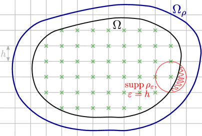
Figure 1. In more than one dimension, it may happen that the support of the smoothing kernel exceeds the boundary of $\Omega$.

Lemma 4.4.

Let $u$ solve eq. 1.1 on a bounded Lipschitz domain that fulfills the exterior ball condition and $f\in L^{\infty}(\Omega)$. For $x\in\Omega^{c}$, let

$$\bar{f}(x)=\operatorname{\mathcal{N}_{s}}u(x)=-C(d,s)\int_{\Omega}\frac{u(y)}{\left|{x-y}\right|^{d+2s}}\mathop{\mathrm{d}y}.$$ (4.51)

Then,

$$\left|{\bar{f}(x)}\right|\leq C_{\text{Bndry.}}(\Omega,s)\cdot\delta(x)^{-s},\quad\delta(x)=\operatorname{dist}(x,\partial\Omega)$$ (4.52)

where $C_{\text{Bndry.}}(\Omega,s)$ is the constant from Theorem 2.1.

Proof.

We know that for $y\in\Omega$ (see eq. 2.16)

$$u(y)\leq C(\Omega,s)\left\|{f}\right\|_{L^{\infty}(\Omega)}\operatorname{dist}(y,\partial\Omega)^{s}.$$ (4.53)

Further, as $x\not\in\Omega$,

$$\operatorname{dist}(y,\partial\Omega)=\inf\limits_{z\in\partial\Omega}\left|{y-z}\right|\leq\left|{y-x}\right|,$$ (4.54)

thus

$$\frac{u(y)}{\left|{x-y}\right|^{d+2s}}\leq C\frac{\operatorname{dist}(y,\partial\Omega)^{s}}{\left|{x-y}\right|^{d+2s}}\leq C\frac{\left|{x-y}\right|^{s}}{\left|{x-y}\right|^{d+2s}}=C\frac{1}{\left|{x-y}\right|^{d+s}}.$$ (4.55)

We plug this into eq. 4.51 to obtain

$$\left|{\bar{f}(x)}\right|\leq C\int_{\Omega}\frac{1}{\left|{x-y}\right|^{d+s}}\mathop{\mathrm{d}y}.$$ (4.56)

To compute this integral, assume w.l.o.g $x=0\not\in\overline{\Omega}$ and choose $R>0$ large enough such that $\Omega\subset B_{R}(0)$, then

$$\int_{\Omega}\frac{1}{\left|{x-y}\right|^{d+s}}\mathop{\mathrm{d}y}=\int_{B_{R}}{\left|{y}\right|^{-(d+s)}}\chi_{\Omega}(y)\mathop{\mathrm{d}y} =\int_{0}^{R}\int_{\mathbb{S}^{d-1}}{\left|{r\xi}\right|^{-(d+s)}}\chi_{\Omega}(r\xi)\mathop{\mathrm{d}o}(\xi)r^{d-1}\mathop{\mathrm{d}r}$$

$$=\int_{0}^{R}r^{-1-s}\int_{\mathbb{S}^{d-1}}\underbrace{\chi_{\Omega}(r\xi)}_{=0\text{ if }r<\delta(x)}\mathop{\mathrm{d}o}(\xi)\mathop{\mathrm{d}r}$$

$$\leq\left|{\mathbb{S}^{d-1}}\right|\frac{1}{-s}\left(R^{-s}-\delta(x)^{-s}\right)\leq\frac{\left|{\mathbb{S}^{d-1}}\right|}{s}\cdot\delta(x)^{-s}.$$ (4.57)

∎

We are ready to prove Theorem 4.1 now.

Proof (of Theorem 4.1).

We split the error into two integrals:

$$\left|{u-u_{\rho}}\right|_{H^{s}(\mathbb{R}^{d})}^{2} \leq\int_{\mathbb{R}^{d}}\underbrace{|(-\Delta)^{s}(u-u_{\rho})|}_{=0\text{ in }\Omega}\cdot\underbrace{|u-u_{\rho}|}_{=0\text{ in }\Omega_{\rho}^{c}}\mathop{\mathrm{d}x}$$

$$=\int_{\Omega_{\rho}\setminus\Omega}\big{|}(-\Delta)^{s}u-\underbrace{(-\Delta)^{s}u_{\rho}}_{=f_{\rho}}\big{|}\cdot|\underbrace{u}_{=0}-u_{\rho}|\mathop{\mathrm{d}x}$$

$$\leq\int_{\Omega_{\rho}\setminus\Omega}|f_{\rho}|\cdot|u_{\rho}|\mathop{\mathrm{d}x}+\int_{\Omega_{\rho}\setminus\Omega}|(-\Delta)^{s}u|\cdot|u_{\rho}|\mathop{\mathrm{d}x}.$$ (4.58)

We bound the integrals individually and obtain for the first integral

$$\int_{\Omega_{\rho}\setminus\Omega}|f_{\rho}|\cdot\left|{u_{\rho}}\right| \leq\left\|{f_{\rho}}\right\|_{L^{\infty}(\Omega_{\rho})}\cdot\int_{\Omega_{\rho}\setminus\Omega}\left|{u_{\rho}}\right|\mathop{\mathrm{d}x}$$

$$\leq\left\|{f_{\rho}}\right\|_{L^{\infty}(\Omega_{\rho})}\cdot C_{\text{Bndry.}}(\Omega_{\rho},f_{\rho})\sup\limits_{x\in\Omega_{\rho}}\underbrace{\operatorname{dist}(x,\partial\Omega_{\rho})^{s}}_{\leq h^{s}}\int_{\Omega_{\rho}\setminus\Omega}1\mathop{\mathrm{d}x}$$

$$\leq\left\|{f_{\rho}}\right\|_{L^{\infty}(\Omega_{\rho})}\cdot C_{\text{Bndry.}}(\Omega_{\rho},f_{\rho})\cdot h^{s}\cdot C(\Omega)h$$ (4.59)

because, with

$$\Omega_{\rho}\setminus\Omega=\bigcup\limits_{t\in(0,h)}\Gamma_{t},\quad\Gamma_{t}\coloneqq\left\{x\in\Omega_{\rho}\setminus\Omega\,|\,\operatorname{dist}(x,\partial\Omega)=t\right\},$$ (4.60)

we have

$$\int_{\Omega_{\rho}\setminus\Omega}1\mathop{\mathrm{d}x}=\int_{0}^{h}\int_{\Gamma_{t}}1\mathop{\mathrm{d}x}\mathop{\mathrm{d}t}\leq\int_{0}^{h}\left|{\Gamma_{h}}\right|h\mathop{\mathrm{d}t}\leq C(\Omega)\cdot h,$$ (4.61)

where $C(\Omega)$ is a constant that depends only on $\Omega$. We reparameterize the second integral using the same parameterization of $\Omega_{\rho}\setminus\Omega$ and Lemma 4.4 to obtain

$$\int_{\Omega_{\rho}\setminus\bar{\Omega}}\left|{(-\Delta)^{s}u}\right|\cdot\left|{u_{\rho}}\right|\mathop{\mathrm{d}x} =\int\limits_{0}^{h}\int_{\Gamma_{t}}\left|{(-\Delta)^{s}u}\right|\cdot\left|{u_{\rho}}\right|\mathop{\mathrm{d}x}\mathop{\mathrm{d}t}\leq C_{\text{Bndry.}}(\Omega_{\rho},f_{\rho})\cdot h^{s}\int\limits_{0}^{h}\int_{\Gamma_{t}}t^{-s}\mathop{\mathrm{d}x}\mathop{\mathrm{d}t}$$

$$=C_{\text{Bndry.}}(\Omega_{\rho},f_{\rho})\cdot h^{s}\int\limits_{0}^{h}\left|{\Gamma_{t}}\right|t^{-s}\mathop{\mathrm{d}t}$$

$$\leq C_{\text{Bndry.}}(\Omega_{\rho},f_{\rho})\cdot h^{s}C(\Omega)h^{1-s}=C_{\text{Bndry.}}(\Omega_{\rho},f_{\rho})C(\Omega)h$$ (4.62)

We plug eqs. 4.59 and 4.62 into eq. 4.58 to obtain

$$\left|{u-u_{\rho}}\right|_{H^{s}(\mathbb{R}^{d})}^{2} \leq C(\Omega)\cdot C_{\text{Bndry.}}(\Omega,f_{\rho})\cdot h^{s+1}+C(\Omega)\cdot C_{\text{Bndry.}}(\Omega,f_{\rho})\cdot h$$

$$\leq 2\,C(\Omega)\cdot C_{\text{Bndry.}}(\Omega,f_{\rho})\cdot h$$ (4.63)

where we used 4.1 which ensures that $C_{\text{Bndry.}}(\Omega_{\rho},f\rho)\leq C\cdot C_{\text{Bndry.}}(\Omega,f\rho)$. This completes the proof.

∎

5. Main theorems

Using the results proven so far, we are finally ready to prove our main theorems.

Theorem 5.1.

Let $\Omega$ be a bounded Lipschitz domain that fulfills Assumption 4.1. Let $f$ be given as in Theorem 2.2 and $u$ solve the exterior value problem eq. 1.1 on $\Omega$. Let $u_{h}\in\mathbb{V}_{h}(\Omega)$ solve the discrete problem, see eq. 1.5, where the right-hand side is chosen as

$$f_{k}=\bar{f}_{\rho,\varepsilon}(x_{k})$$

for $k/N\in\Omega$. Let $\rho=\sqrt{d}h$ and $\Omega_{\rho}$, $f_{\rho}$, $u_{\rho}$ and $\bar{f}_{\rho}$ as described in Section 4.3 and $\bar{f}_{\rho,\varepsilon}$ is obtained as a mollification of $\bar{f}_{\rho}$, see eq. 3.28, with the mollifier constructed in appendix A. Then, with $\theta=1/\left|{\log(h)}\right|$ as in [2],

$$\left\|{u-u_{h}}\right\|_{H^{s}({\mathbb{R}^{d}})} \leq C\cdot\Big{(}C_{\text{Sob.}}(\Omega,f)+C_{\text{Bndry.}}(\Omega,f)+C_{\text{Sob.}}(\Omega_{\rho},f_{\rho})+C_{\text{Bndry.}}(\Omega_{\rho},f_{\rho})\Big{)}\cdot\frac{h^{1/2-\theta}}{\theta}$$

$$=C\cdot\Big{(}C_{\text{Sob.}}(\Omega,f)+C_{\text{Bndry.}}(\Omega,f)+C_{\text{Sob.}}(\Omega_{\rho},f_{\rho})+C_{\text{Bndry.}}(\Omega_{\rho},f_{\rho})\Big{)}\left|{\log(h)}\right|h^{1/2}$$

where $C$ depends on $\Omega,s$ and $d$.

Proof.

This is a direct consequence of the results proven so far. Using the abstract error estimate, see Theorem 3.1, we obtain that

$$\left\|{u-u_{h}}\right\|_{H^{s}({\mathbb{R}^{d}})}\leq\left(1+\frac{C}{\gamma}\right)\inf\limits_{v_{h}\in\mathbb{V}_{h}(\Omega)}\left\|{u-v_{h}}\right\|_{H^{s}({\mathbb{R}^{d}})}+\frac{1}{\gamma}\sup\limits_{w_{h}\in\mathbb{V}_{h}(\Omega)\setminus\{0\}}\frac{\left|{a(u-u_{h},w_{h})}\right|}{\left\|{w_{h}}\right\|_{H^{s}({\mathbb{R}^{d}})}}$$ (5.1)

The bound for the first term is a direct consequence of Proposition 4.1. The numerator of the second term can be bounded after adding appropriate zeros and using the triangle inequality by

$$\left|{a(u-u_{h},w_{h})}\right|\leq\left(\left|{u-u_{\rho}}\right|_{H^{s}(\mathbb{R}^{d})}+\left\|{\bar{f}_{\rho}-\bar{f}_{\rho,\varepsilon}}\right\|_{H^{-s}(\mathbb{R}^{d})}+\left\|{\bar{f}_{\rho,\varepsilon}-\operatorname{\Pi_{N}}f_{\rho,\varepsilon}}\right\|_{H^{-s}(\mathbb{R}^{d})}\right)\cdot\left\|{w_{h}}\right\|_{H^{s}({\mathbb{R}^{d}})}$$ (5.2)

Now, the desired bound follows by applying Theorem 4.1 to the first term of the sum and Lemma 4.3 to the second and third term, and further noticing that we set $\rho=\sqrt{d}h$. ∎

We acknowledge that although, in principle, theorem 5.1 gives an appropriate error bound, actually obtaining a right-hand side with the extension-and-mollification approach may be challenging in practice. However, if we assume that $f$ has some more regularity in $\Omega$, we can enhance the previous result and show that we can indeed obtain the right-hand side of the discrete system by simple direct sampling, i.e., setting $f_{k}=f(k/N)$ for $k/N\in\Omega$.

Theorem 5.2.

Let the setting be as in Theorem 5.1 and let, additionally, $f\in C^{1/2}(\overline{\Omega})$. Let the entries of the right-hand side in eq. 1.5 be chosen as

$$f_{k}=f(k/N)$$

for $k/N\in\Omega$. Then,

$$\left\|{u-u_{h}}\right\|_{H^{s}({\mathbb{R}^{d}})} \leq C\cdot\Big{(}C_{\text{Sob.}}(\Omega,f)+C_{\text{Bndry.}}(\Omega,f)+C_{\text{Sob.}}(\Omega_{\rho},f_{\rho})+C_{\text{Bndry.}}(\Omega_{\rho},f_{\rho})\Big{)}\cdot\frac{h^{1/2-\theta}}{\theta}$$

$$=C\cdot\Big{(}C_{\text{Sob.}}(\Omega,f)+C_{\text{Bndry.}}(\Omega,f)+C_{\text{Sob.}}(\Omega_{\rho},f_{\rho})+C_{\text{Bndry.}}(\Omega_{\rho},f_{\rho})\Big{)}\left|{\log(h)}\right|h^{1/2}$$

where $C$ depends on $\Omega,s$ and $d$.

Proof.

The arguments are in essence the same as in the proof of Theorem 5.1. The additional term we have to bound in the consistency term is

$$(\operatorname{\Pi_{N}}f_{\rho}-\operatorname{\Pi_{N}}f_{\rho,\varepsilon},w_{h})_{L^{2}({\mathbb{R}^{d}})}\leq\left(N^{-d}\sum\limits_{k/N\in\Omega}(f_{\rho}(x_{k})-f_{\rho,\varepsilon}(x_{k}))^{2}\right)^{1/2}\cdot\left\|{w_{h}}\right\|_{L^{2}(\mathbb{R}^{d})}$$ (5.3)

First, note that we extend $f$ to $f_{\rho}\in C^{1/2}(\Omega_{\rho})$ as before. Then, for $x_{k}\in\Omega$,

$$\left|{f_{\rho,\varepsilon}(k/N)-f_{\rho}(k/N)}\right| =\left|\int_{B_{\varepsilon}(x)}\eta_{\varepsilon}(x-y)(f_{\rho}(x)-f_{\rho}(y))\mathop{\mathrm{d}y}\right|$$

$$\leq\int_{B_{\varepsilon}(x)}\eta_{\varepsilon}(x-y)\mathop{\mathrm{d}y}\sup\limits_{y\in B_{\varepsilon}(x)}|f_{\rho}(x)-f_{\rho}(y)|$$

$$\leq C\left|{x-y}\right|^{1/2}\leq C\varepsilon^{1/2}.$$

Plugging this into eq. 5.3 and setting $\varepsilon=h$ gives the desired result. ∎

If the domain has not only a Lipschitz boundary but a smooth boundary, we can obtain error boundaries also without the assumption that $f$ is Hölder continuous.

Theorem 5.3.

Let $\Omega$ be a smooth domain that fulfills Assumption 4.1 and let $f\in L^{\infty}(\Omega)$. Let $u$ solve the exterior value problem eq. 1.1 on $\Omega$. Let $u_{h}\in\mathbb{V}_{h}(\Omega)$ solve the discrete problem, see eq. 1.5, where the right-hand side is chosen as

$$f_{k}=\bar{f}_{\rho,\varepsilon}(x_{k}).$$

Then,

$$\left\|{u-u_{h}}\right\|_{H^{s}({\mathbb{R}^{d}})}\leq C\cdot\Big{(}C_{\text{Sob.}}(\Omega,f)+C_{\text{Bndry.}}(\Omega,f)+C_{\text{Sob.}}(\Omega_{\rho},f_{\rho})+C_{\text{Bndry.}}(\Omega_{\rho},f_{\rho})\Big{)}\cdot\frac{1}{\theta}h^{\alpha}.$$

In case $s<\frac{1}{2}$, we have $\alpha=s$ and $C$ is a constant that depends on $\Omega,d$ and $s$.

In case $s\geq\frac{1}{2}$, we have $\alpha=\frac{1}{2}-\theta$ for all $\theta>0$ and $C$ is a constant that depends on $\Omega,d,s$ and $\alpha$.

Proof.

The proof is essentially the same as for Theorems 5.1 and 5.2 using Proposition 4.2 and that we can extend $f\in L^{\infty}(\Omega)$ to $f_{\rho}\in L^{\infty}(\Omega_{\rho})$. ∎

Remark 5.1.

The main ingredients to prove the theorems above are Sobolev regularity and decay near the boundary of solutions $u$. Thus it is easily possible to derive similar results for specific cases where regularity and decay estimates are also available, with sub-error decay rates depending on regularity and boundary decay rate. A possible application are convergence results on (not necessarily smooth) Lipschitz domains that fulfill the exterior ball condition for $f\in L^{\infty}(\Omega)\subset L^{2}(\Omega)$ using the results shown in [9, 10]

Appendix A Construction of appropriate mollifiers

The above estimates for the approximation of the right-hand side only give us the desired rate if we can bound the constant $C$ in eq. 4.43 appropriately. This is achieved if the sum

$$\sum_{k\neq 0}\hat{\eta}\left(2\pi(k+\omega)\right)^{2}|(k+\omega)|^{2s}$$ (A.1)

(i) is finite and (ii) sufficiently small around ${\omega=0}$. We achieve this as follows. We want to have a mollifier $\eta(x)$ such that

$$\hat{\eta}(\omega)=\hat{\psi}(\omega)\cdot S(\omega)$$ (A.2)

where

$$S(\omega)=\prod\limits_{i=1}^{d}\operatorname{sinc}(\omega_{i}/(2\pi))$$ (A.3)

and $\hat{\psi}(\omega)\rightarrow 0$ as $\left|{\omega}\right|\rightarrow\infty$ fast enough to ensure that the sum in eq. A.1 remains bounded. Precisely, the mollifier $\eta$ is obtained as the convolution of $\psi$ and $\check{S}\coloneqq\operatorname{\mathcal{F}^{-1}}S$, which gives the structure of the mollifier, see eq. A.2, through the convolution theorem for the Fourier transformation. Set

$$\check{S}=\chi_{(-1/2,1/2)^{d}}(x)=\begin{cases}1&\text{if }x\in(-1/2,1/2)^{d}\\ 0&\text{otherwise}\end{cases},$$ (A.4)

the indicator function on the cube from $-1/2$ to $1/2$ in each spatial direction. Note that for this definition, $S=\operatorname{\mathcal{F}}{\check{S}}$ is exactly fulfilled. It is clear that $\operatorname{supp}{\check{S}}\subset B_{\sqrt{d}/2}$. Thus clearly, if we choose $\psi$ to be a smooth mollifier and scale its support to a circle of radius $\sqrt{d}/4$, we have $\operatorname{supp}{\check{S}*\psi}\subset B_{\sqrt{d}}$. Further, we have to normalize $\psi$ such that $\int_{\mathbb{R}^{d}}\left(\psi*\check{S}\right)\mathop{\mathrm{d}x}=1$. As we assume $\psi\subset C_{c}^{\infty}({\mathbb{R}^{d}})$, we can assume $\hat{\psi}(\omega)\leq C\exp(-\omega)$. The so constructed mollifier in $d=2$ is shown in fig. 2.

The second factor in eq. A.2 ensures that the sum in eq. 4.43 is $0$ if $\omega=0$, the first ensures that it remains bounded. To show this, note that for the mollifier as defined in equations eqs. A.2 and A.3, it holds that

$$\sum\limits_{k\neq 0}\hat{\eta}(2\pi(k+\omega))^{2}|k+\omega|^{2s} =\sum\limits_{k\neq 0}\left(S(2\pi(k+\omega))\hat{\psi}(2\pi(k+\omega))\right)^{2}|k+\omega|^{2s}$$

$$=\sum\limits_{k\neq 0}\left(\prod\limits_{i=1}^{d}\frac{\sin(\pi(k_{i}+\omega_{i}))}{\pi(k_{i}+\omega_{i})}\right)^{2}\hat{\psi}^{2}(2\pi(k+\omega))|k+\omega|^{2s}$$

$$=\prod\limits_{i=1}^{d}\left(\frac{\sin(\pi\omega_{i})}{\pi}\right)^{2}\sum\limits_{k\neq 0}\prod\limits_{i=1}^{d}\frac{1}{(k_{i}+\omega_{i})^{2}}\hat{\psi}^{2}(2\pi(k+\omega))|k+\omega|^{2s}$$

$$\leq C\prod\limits_{i=1}^{d}\left(\frac{\sin(\pi\omega_{i})}{\pi}\right)^{2}\sum\limits_{k\neq 0}\frac{\exp(-4\pi\left|{k+\omega}\right|)\cdot|k+\omega|^{2s}}{\prod_{i=1}^{d}(k_{i}+\omega_{i})^{2}}$$

$$\leq C\prod\limits_{i=1}^{d}\omega_{i}^{2}\underbrace{\sum\limits_{k\neq 0}\frac{\exp(-4\pi\left|{k+\omega}\right|)\cdot|k+\omega|^{2s}}{\prod_{i=1}^{d}(k_{i}+\omega_{i})^{2}}}_{\leq\text{const.}}$$

$$\leq C\prod\limits_{i=1}^{d}\omega_{i}^{2}\leq C\left|{\omega}\right|^{2d}$$ (A.5)

where $C$ is a varying constant that depends on the decay of $\hat{\psi}$, $s$ and $d$. For the last inequality, we used the generalized mean inequalities. We plug this into eq. 4.43 and obtain

$$\frac{(2N\pi)^{2s}}{w(2N\pi\omega)^{s}}\sum\limits_{k\neq 0}\hat{\eta}\left(2\pi(k+\omega)\right)^{2}|(k+\omega)|^{2s}\leq C\frac{1}{\left(1/(2N\pi)^{2}+\left|{\omega}\right|^{2}\right)^{s}}\left|{\omega}\right|^{2d}\leq\left|{\omega}\right|^{2d-2s}<\infty$$ (A.6)

if $s<d$.

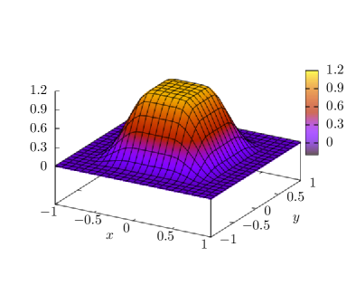
Figure 2. The mollifier constructed as $\eta(x)=(S*\psi)(x)$ and normalized s.t. $\int_{\mathbb{R}^{d}}\eta\mathop{\mathrm{d}x}=0$ in $d=2$.

References

- [1] Helmut Abels and Gerd Grubb. Fractional-order operators on nonsmooth domains. Journal of the London Mathematical Society, 107(4):1297–1350, January 2023.
- [2] Gabriel Acosta and Juan Pablo Borthagaray. A fractional Laplace equation: Regularity of solutions and finite element approximations. SIAM Journal on Numerical Analysis, 55(2):472–495, Jan 2017.
- [3] Mark Ainsworth and Christian Glusa. Aspects of an adaptive finite element method for the fractional Laplacian: A priori and a posteriori error estimates, efficient implementation and multigrid solver. Computer Methods in Applied Mechanics and Engineering, 327:4–35, 2017. Advances in Computational Mechanics and Scientific Computation—the Cutting Edge.
- [4] Mark Ainsworth and Christian Glusa. Towards an efficient finite element method for the integral fractional Laplacian on polygonal domains. In Josef Dick, Frances Y. Kuo, and Henryk Woźniakowski, editors, Contemporary Computational Mathematics - A Celebration of the 80th Birthday of Ian Sloan, pages 17–57. Springer International Publishing, Cham, 2018.
- [5] Harbir Antil, Patrick Dondl, and Ludwig Striet. Approximation of integral fractional Laplacian and fractional PDEs via sinc-basis. SIAM Journal on Scientific Computing, 43(4):A2897–A2922, 2021.
- [6] Igor Belegradek and Zixin Jiang. Smoothness of minkowski sum and generic rotations. Journal of Mathematical Analysis and Applications, 450(2):1229–1244, 2017.
- [7] Andrea Bonito, Juan Pablo Borthagaray, Ricardo H. Nochetto, Enrique Otárola, and Abner J. Salgado. Numerical methods for fractional diffusion. Computing and Visualization in Science, 19(5-6):19–46, mar 2018.
- [8] Andrea Bonito, Wenyu Lei, and Joseph E. Pasciak. Numerical approximation of the integral fractional Laplacian. Numerische Mathematik, 142(2):235–278, February 2019.
- [9] Juan Pablo Borthagaray, Dmitriy Leykekhman, and Ricardo H. Nochetto. Local energy estimates for the fractional Laplacian. SIAM Journal on Numerical Analysis, 59(4):1918–1947, 2021.
- [10] Juan Pablo Borthagaray and Ricardo H. Nochetto. Besov regularity for the Dirichlet integral fractional Laplacian in Lipschitz domains, 2021.
- [11] Juan Pablo Borthagaray, Leandro M. Del Pezzo, and Sandra Martinez. Finite element approximation for the fractional eigenvalue problem. Journal of Scientific Computing, 77(1):308–329, April 2018.
- [12] S. Brenner and R. Scott. The Mathematical Theory of Finite Element Methods. Texts in Applied Mathematics. Springer New York, 2007.
- [13] Giovanni Covi, Keijo Mönkkönen, and Jesse Railo. Unique continuation property and Poincaré inequality for higher order fractional Laplacians with applications in inverse problems. arXiv e-prints, page arXiv:2001.06210, January 2020.
- [14] Eleonora Di Nezza, Giampiero Palatucci, and Enrico Valdinoci. Hitchhikers guide to the fractional sobolev spaces. Bulletin des Sciences Mathématiques, 136(5):521–573, 2012.
- [15] Serena Dipierro, Xavier Ros-Oton, and Enrico Valdinoci. Nonlocal problems with Neumann boundary conditions. Revista Matematica Iberoamericana, 33:377+, Jun 2017. 2.
- [16] Siwei Duo and Yanzhi Zhang. Accurate numerical methods for two and three dimensional integral fractional Laplacian with applications. Computer Methods in Applied Mechanics and Engineering, 355:639 – 662, 2019.
- [17] Marta D’Elia and Max Gunzburger. The fractional laplacian operator on bounded domains as a special case of the nonlocal diffusion operator. Computers & Mathematics with Applications, 66(7):1245–1260, 2013.
- [18] Alexandre Ern and Jean-Luc Guermond. Finite Elements II. Springer International Publishing, 2021.
- [19] David Gilbarg and Neil S. Trudinger. Elliptic Partial Differential Equations of Second Order. Springer Berlin Heidelberg, 2001.
- [20] Loukas Grafakos. Classical Fourier Analysis. Graduate Texts in Mathematics. Springer, New York, NY, October 2010.
- [21] Rubing Han and Shuonan Wu. A monotone discretization for integral fractional laplacian on bounded lipschitz domains: Pointwise error estimates under hölder regularity. SIAM Journal on Numerical Analysis, 60(6):3052–3077, 2022.
- [22] Zhaopeng Hao, Zhongqiang Zhang, and Rui Du. Fractional centered difference scheme for high-dimensional integral fractional laplacian. Journal of Computational Physics, 424:109851, 2021.
- [23] Luca Heltai and Wenyu Lei. A priori error estimates of regularized elliptic problems. Numerische Mathematik, 146(3):571–596, September 2020.
- [24] Yanghong Huang and Adam Oberman. Numerical methods for the fractional laplacian: A finite difference-quadrature approach. SIAM Journal on Numerical Analysis, 52(6):3056–3084, 2014.
- [25] Yanghong Huang and Adam Oberman. Finite difference methods for fractional Laplacians. arXiv e-prints, page arXiv:1611.00164, November 2016.
- [26] Michael Karkulik and Jens Markus Melenk. $\mathscrh$-matrix approximability of inverses of discretizations of the fractional laplacian. Advances in Computational Mathematics, 45(5-6):2893–2919, November 2019.
- [27] Mateusz Kwaśnicki. Ten equivalent definitions of the fractional Laplace operator. Fractional Calculus and Applied Analysis, 20, 07 2015.
- [28] Victor Minden and Lexing Ying. A simple solver for the fractional Laplacian in multiple dimensions. SIAM Journal on Scientific Computing, 42(2):A878–A900, 2020.
- [29] Ha Q Nguyen, Michael Unser, and John Paul Ward. Generalized poisson summation formulas for continuous functions of polynomial growth. Journal of Fourier Analysis and Applications, 23:442–461, 2017.
- [30] Xavier Ros-Oton and Joaquim Serra. The Dirichlet problem for the fractional Laplacian: Regularity up to the boundary. Journal de Mathématiques Pures et Appliquées, 101(3):275 – 302, 2014.
- [31] F. Stenger. Handbook of Sinc Numerical Methods. Chapman & Hall/CRC Numerical Analysis and Scientific Computing Series. CRC Press, 2011.