Numerical approximations of thin structure deformations
Abstract.
We review different (reduced) models for thin structures using bending as principal mechanism to undergo large deformations. Each model consists in the minimization of a fourth order energy, potentially subject to a nonconvex constraint. Equilibrium deformations are approximated using local discontinuous Galerkin (LDG) finite elements. The design of the discrete energies relies on a discrete Hessian operator defined on discontinuous functions with better approximation properties than the piecewise Hessian. Discrete gradient flows are put in place to drive the minimization process. They are chosen for their robustness and ability to preserve the nonconvex constraint. Several numerical experiments are presented to showcase the large variety of shapes that can be achieved with these models.
Key words and phrases:
Keywords: Nonlinear elasticity; plate deformation; folding; prestrain metric; discontinuous Galerkin; reconstructed Hessian; numerical simulations1991 Mathematics Subject Classification:
AMS Subject Classification: 65N12, 65N30, 74K20, 74G651. Introduction
Deformations of thin materials are widely observed in nature, from the snapping of the venus flytrap [29, 62] to the natural growth of soft tissues in leaves and flowers [35, 69, 13, 47]. They also appear in a variety of man-made applications [41, 42]. Some thin structures, called bilayers, are made of two thin layers of different materials that react differently to external stimuli (changes in temperature or humidity, electrical or chemical stimuli, etc.). Examples include the bimetal strips in thermostats, microactuators [38, 11], and plywood panels in climate-responsive architectures [52] inspired from the morphology of conifer cones. Bending of thin sheets can also occur when folding is present; examples of this include origami and flexible structures [63, 49]. We refer to the review paper [47] for additional examples.
All the phenomena listed above can be modelled as thin limits of hyperelastic materials. A thin structure of thickness endowed with a hyperelastic energy is approximated by its two dimensional midplane endowed with a limiting energy as the thickness vanishes. A hierarchy of reduced models for elastic deformations is described in [33], in which the type of the model depends on the scaling of the elastic energy with the thickness of the plate. The scaling corresponds to stretching, the scaling corresponds to bending, and the scaling corresponds to the von Kármán theory of plate bending. Each of these reduced energies are the -limit of . We refer to [46] for the membrane theory, to [34, 32, 30] for the bending theory, and to [31, 33] for the von Kármán theory. In particular, cluster points of sequences of minimizers of are minimizers of the -limit.
In this work, we are mainly interested in the bending regime, namely when the hyperelastic three dimensional energy
| (1) |
scales like the cube of the thickness of the plate . Here, is the midplane of the thin structure, is a deformation of the plate, is a prescribed Riemannian metric (deformations satisfying the target metric are stress-free), and is some energy density function satisfying [32]
-
•
, in a neighborhood of ;
-
•
is frame indifferent: for all and all ;
-
•
for all and if ,
where denotes the special orthogonal group of rotations in . In this work, we restrict our considerations to the St. Venant-Kirchhoff stored energy, see (8).
The prestrain metric characterizes the material. From the third property of the energy density, we see that when is the identity matrix, the minimum of the hyperelastic energy (1) (without boundary conditions or external forces) is zero and is achieved by rigid motions. That is, at equilibrium, the plate is stress free and flat. When the Riemannian curvature tensor of is not identically zero, then the minimum of the hyperelastic energy is strictly positive [48]. In this case, there is no stress-free configuration. The plate is then said to be non-Euclidean or prestrained and generally exhibits more complex equilibrium shapes.
In 1850, Kirchhoff [40] obtained a reduced energy that can be formally obtained assuming that the material deformation reads
| (2) |
where is the normal to the deformed midplane . This assumption, used by Love [50], is usually referred to as (nonlinear) Kirchhoff-Love ansatz in the literature, although it is not due to Kirchhoff [32]. When the thickness of the plate is small, it is convenient to derive reduced models for the deformation of the midplane . In [28], see also [13], the Kirchhoff-Love assumption (2) is made for prestrained plates. The resulting model consists of the sum of a stretching and a bending component multiplied by different powers of the plate thickness . We derive a similar energy referred to as the preasymptotic energy to express that it is obtained upon assuming that is small but not vanishing. To do this, we follow [48] and assume that
| (3) |
i.e. is uniform within the thickness and no stretching occurs in the direction orthogonal to the plane. The function is assumed to be symmetric and uniformly positive definite.
The vanishing thickness limit of prestrained materials has been studied in several works. When is the identity matrix, as mentioned above, a reduced energy was obtained formally by Kirchhoff [40]. Much later, an ansatz-free derivation was obtained via -convergence in the seminal work [32]. The limiting energy involves the second fundamental form of the midplane deformation and is finite only for isometric immersions.
For the derivation in the general case, namely when is not the identity matrix, we refer to [48, 13, 14, 51, 15]. The first -convergence results for prestrained plates were obtained in [48] for target metrics as in (3), and later extended to more general metrics in [14]. In both cases, the metric is assumed to be independent of the thickness and uniform throughout the thickness. For the particular metric given in (3), the limiting energy involves the second fundamental form of the midplane deformation and is finite only for isometric immersion of the two dimensional target metric . In [17] a formal derivation based on a modified Kirchhoff-Love assumption (2) of the reduced model is provided.
Bilayer materials are composed of two thin layers of materials with different properties. External (thermal, electrical or chemical) stimuli correspond to a prestrain metric
| (4) |
where the product describes the lattice mismatch between the layers, and encodes the inhomogeneity and anisotropy of the bilayer. When actuated, the material deforms to relax its internal stress and can typically undergo large deformations even with relatively small stimuli. The reduced model for bilayer plates was derived via -convergence in [64] and formally explained in [7] for a metric of the form (4). The limiting energy penalizes deviations of the second fundamental form of the midplane from a spontaneous curvature which depends on the mismatch between the two layers (i.e. on and ). In this model, as in the others when , the energy is finite only when the deformations are isometries.
The ability of the plate to fold along creases was incorporated in [6]. It considers hyperelastic materials with assumed to be weakened in a neighborhood of a curve modelling a crease. Assuming an asymptotic behavior of the defect width and strength (see (28)), the limiting model reduces to the original model without the crease, except that jumps on the deformations gradients are allowed across the crease without suffering any energetic penalty. Note that in principle, any plate - with an isometry constraint or prestrain, a single layer or a bilayer - can have folding. However, only the case of a single layer plate with isometry has been derived rigorously so far.
Motivations and Novelties.
One of the goals of this paper is to review different models for the deformation of plates, including single layer and bilayer plates, plates with an isometry constraint as well as general prestrain metric constraints, and plates with folding along some curves inside the domain. Although emphasis is made on the pure bending of plates, the preasymptotic regime, in which both the bending and the stretching/shearing of the plate are considered, is also analyzed. To give an intuitive derivation, the reduced two dimensional energies are obtained formally using a (modified) Kirchhoff-Love assumption for the deformation of the three dimensional plate. However, as mentioned above, ansatz-free limiting energies have been obtained via -convergence for most cases.
A second goal is to collect in one place the numerical methods proposed recently by the authors and collaborators for the approximation of near minimizers of the discrete energies. These methods are based on a local discontinuous Galerkin (LDG) approach for the space discretization and a gradient flow for the minimization of the discrete energy. This methodology has already been successfully applied to a wide range of problems, see for instance [17, 22, 6]. Moreover, the -convergence as the mesh size goes to zero of the discrete energies obtained using LDG is analyzed in [16], [18], [22], and [6] for the preasymptotic, prestrain, bilayer, and folding case, respectively. Note that other discretizations are also possible. We refer to [20, 21, 8] for approaches using the symmetric interior penalty discontinuous Galerkin method, and to [4, 7, 9, 5] for a method based on Kirchhoff elements.
This work also offers several novel contributions. We present a recently developed algorithm for the preasymptotic model, extend the existing algorithms to time-dependent input data, present a uniform treatment of folding effects, and introduce an accelerated algorithm that drastically improves the performance of the unconstrained discrete gradient flows. We perform new and challenging simulations highlighting the various types of deformations that can be achieved with the models, as well as the versatility of the code.
Outline.
The rest of this paper is organized as follows. In Section 2, we formally derive the various two dimensional models for the deformation of thin structures and discuss how to incorporate forcing and boundary conditions into these models. In Section 3, we present the spatial discretization of the two dimensional energies based on the LDG method, including the introduction of a discrete Hessian operator - the key component of the method. The discrete gradient flows put forward to minimize the discrete energies are described in Section 4, which also includes strategies to produce good initial deformations and to potentially improve the convergence rate of the iterative processes. Section 5 is devoted to numerical experiments demonstrating the variety of deformations that can be achieved.
Notation.
In what follows, we will denote by the identity matrix in . Moreover, for a multivariate function, we write the partial derivative with respect to the variable. Uppercase letters and bold lowercase letters will be used for matrix-valued and vector-valued functions, respectively, and subindices will denote their components. For instance, the component of will be denoted , and , while the component of will be denoted , . Furthermore, for , will denote the row of , . For , the divergence operator is applied row-wise, namely for . Finally, we use the notation to denote the Euclidean scalar product between two tensors and for the corresponding Frobenius norm. For the particular case of vectors, the Euclidean scalar product between is instead denoted by .
2. Mathematical Models
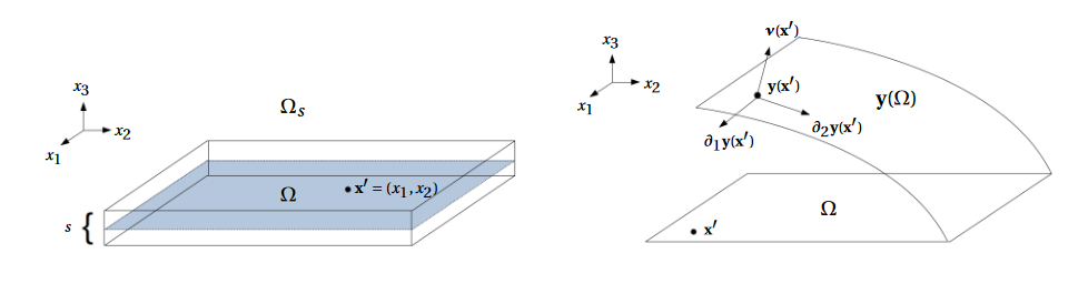
In this section, we provide a formal but intuitive derivation of two dimensional models for three dimensional thin hyperelastic structures. References to rigorous derivations of the bending model with isometry and prestrain constraint and of the bilayer model via -convergence can be found in Sections 2.2, 2.3, and 2.4, respectively. The thin structure is denoted , where stands for the thickness of the structure and is a open, bounded domain with Lipschitz boundary which represents the midplane (see the diagram on the left of Figure 1). A deformation of the plate is denoted by while its restriction to the midplane is denoted (see the diagram on the right of Figure 1). For later use, we also introduce the unit normal vector to the surface at the point
and the first and second fundamental forms of the surface
| (5) |
Here denotes the gradient with respect to the variable .
In all the models presented below, the structure is endowed with an energy favoring deformations with Cauchy-Green strain tensor matching a given target metric (symmetric and positive definite), i.e. for which the strain tensor
| (6) |
is as close to zero as possible. Note that signifies that the first fundamental form of the deformed surface is and that is an isometric immersion of . Whether a given dimensional Riemannian manifold has an isometric immersion into is a long standing problem in differential geometry, see for instance [37, 25]. By the Nash-Kuiper embedding theorem [56, 43, 44], there always exists an isometric immersion of in . However, the deformation cannot be orientation preserving unless the Riemannian curvature tensor of is identically zero, see [47] and the references therein.
2.1. Bending of Isotropic Thin Structures
We start by considering thin structures endowed with the isotropic hyperelastic energy
| (7) |
where is the St. Venant-Kirchhoff stored energy density function defined by
| (8) |
Here is the deformation gradient assumed to satisfy the orientation condition , is the Green-Lagrange strain tensor corresponding to in (6), and and are the Lamé constants. As we shall see below, deformations for which scales like correspond to a stretching of the midplane (membrane theory), while bending occurs when scales like (bending theory).
Note that in absence of other constraints such as boundary conditions or external forcing, energy (7) is minimized on , i.e. when the deformations are isometries:
2.2. Limiting Model and Modified Kirchhoff Assumption
Two dimensional models for hyperelastic thin structures are derived in [32]. It is shown that when bending is the chief mechanism of deformations, the energy must scale like and
where for
| (9) |
Part of the -convergence argument provided in [32] is based on the construction of a recovery sequence given for and by
| (10) |
for a midplane deformation with finite energy . This indicates that the two dimensional model (9) requires that the fibers orthogonal to the midplane are not stretched homogeneously on . This differentiates the theory in [32] from the standard Cosserat (or Kirchhoff-Love) theory based on the ansatz
and leading to the same two dimensional energy improperly scaled with coefficient instead of in front of the trace term [34, 32].
2.2.1. Preasymptotic
We follow [17] and provide a formal derivation of the preasymptotic energy for thin structures with non-vanishing but small thickness under assumption (10) on the deformations. We are interested in deformations where bending is the chief mechanism and thus also fix and assume that
| (11) |
for a constant independent of . We recall that stands for the gradient with respect to so that
Because for and , we have
and thus
We rewrite the above expression using the first and second fundamental forms (5) of the deformed midplane . In addition, we take advantage of the symmetry of the second fundamental form to obtain
| (12) |
where
Using this relation in the energy density (8) with , we obtain
Note that the terms with odd power of vanish when integrating on to derive an expression of the energy (7). Thus, we get
The terms with and are of higher order. Indeed, thanks to the scaling assumption (11), we have
where is independent of . A similar argument holds for the trace terms. As a consequence, in view of the definitions of and in (12), the expression (5) for the first and second fundamental forms, and the definition of in (10), we arrive at the final expression for the three dimensional energy per unit volume :
| (13) |
where
denote the stretching and bending energies, respectively.
2.2.2. Limiting Bending Model
We are now interested in taking the limit when . We recall that we are assuming (11), which, as we shall see, implies that the limiting plate deformation can not stretch nor shear the midplane but can bend it to reduce its energy.
The starting point to derive the limiting energy as the thickness vanishes is the preasymptotic expression (13) for the energy. The bending regime condition (11) implies that and
| (14) |
Note that when ,
i.e. is an isometry and in particular . Furthermore, for isometries the following relations for the second fundamental form hold (see for instance [4]):
| (15) |
This allows to rewrite the limiting energy as
| (16) |
when is an isometry, i.e. , and where .
2.3. Single Layer with a General Metric Constraint
Without additional constraints such as boundary conditions, the minimum of energy (7) with density (8) is achieved by the identity deformation , which is an isometry. In particular, the reference flat configuration is stress-free. We now consider prestrained materials characterized by the presence of internal stresses in the flat configuration. Examples are nematic glasses [53, 54], natural growth of soft tissues [35, 69], and manufactured polymer gels [39, 41, 68].
We follow [48, 14] (see also [17]) and modify the energy (7) to read
| (17) |
where is a given symmetric positive definite target metric and denotes the positive definite symmetric square root of the inverse of . Note that the previous case is recovered when . Furthermore, when is a metric immersion, i.e. there exists a deformation such that
| (18) |
we have
and thus is a minimizer of with .
Following [28, 48], we further assume that has the form
| (19) |
where is symmetric and uniformly positive definite. In other words, the metric is independent of the variable , is uniform throughout the thickness, and no stretching is allowed in the vertical direction.
The -convergence of this model towards the two dimensional energy given below is obtained in [48, 14]. Proceeding as in Section 2.2.1, an intuitive derivation of the two dimensional -limit can be obtained, using again assumption (10). Indeed, when , neglecting the terms the three dimensional prestrain energy, (17) satisfies
| (20) |
where
| (21) |
and
| (22) |
Note that we slightly abuse the notation by using to refer to both the three dimensional and two dimensional prestrain energy. Which energy is referring to will be clear from the context.
For the limit to be finite as the thickness goes to zero, the two dimensional deformation must satisfy the metric constraint
| (23) |
and in that case
| (24) |
Remark 1.
Nash’s theorem guarantees that there exists an isometric immersion of into [36], but whether or not there exists an isometric immersion into depends on . We refer to [37] for a discussion of positive and negative results for metrics with specific properties. Note that the existence of satisfying (23) is equivalent to the boundedness condition (11) on . We refer to [48] for the case where has the form (19) and to [45] for a general Riemannian metric.
Comparing the limiting energy (24) with (14), we find that the isometry case is recovered for . However, in the case of isometries, the energy is further reduced to (16) thanks to (15). When , the second fundamental form of in (24) cannot be substituted by the Hessian of . Nevertheless, Proposition 1 in [17] and Proposition A.1 in [18] guarantee that for and , up to an additive term only depending on , the limiting energy (24) is equal to
where is the component of . In addition, in view of the metric constraint (23) we have . As a consequence, the equilibrium deformations of the thin limit of prestrained materials are deformations satisfying and minimizing
| (25) |
2.4. Bilayer Plates
We now discuss an anisotropic model where the three dimensional hyperelastic structure is a compound of two thin layers with different mechanical properties. Each material exhibits a different response under external stimuli, generating a material mismatch compensated by the bending of the structure. Temperature, humidity, pH, and electric current are typical external stimuli. We refer for instance to [65, 38, 1, 3] for devices actuated by electric current and to [52, 67] for humidity controlled materials.
From a mathematical point of view, this corresponds to a prestrain tensor of the form
| (26) |
where the inhomogeneity and anisotropy of the bilayer material is encoded in the tensor
with uniformly symmetric, , and . Note that the expression (26) does not reduce to the previous setting with target metric (18).
The limiting model is derived in [64] via -convergence when and can again be formally recovered using a modified Kirchhoff-Love assumption, namely
with
Proceeding as in the previous section, the limiting energy as the thickness goes to zero is
provided that is an isometry, where the constant depends on , , , and , but not on the deformation . We refer to [7] for more details in the case and .
In what follows, we consider an equivalent limiting two dimensional energy
for and with . Note that acts as an intrinsic spontaneous curvature tensor favoring deformations with principal curvatures matching the eigenvalues of . Now recall that the entries of the second fundamental form are given by
and is thus nonlinear in . Taking advantage of relation (15) valid for isometries, we have
which allows us to write
Deformations of bilayer materials are thus deformations satisfying and minimizing
| (27) |
2.5. Folding
We incorporate the capability for the plates to fold along a given crease. In particular, we make structural assumptions leading to a limiting model for which folding does not require any energy. We restrict our description to single layer plates with isometry constraint (i.e. ). The derivation of the folding model described here was originally proposed in [6]. Extensions to other models, although feasible, have not been treated in the existing literature. However, numerical simulation are available in [22] for the bending of a bilayer plate with folding.
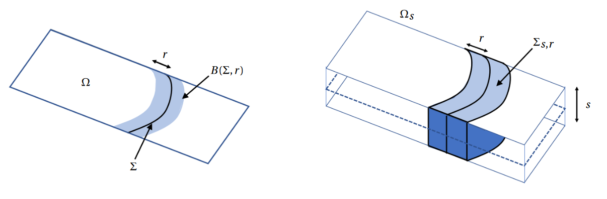
Folding models are obtained by assuming that the thin structure has a material defect in a cylindrical neighborhood of a curve (the crease) splitting in two parts and intersecting the boundary transversely. Let be as above and let be the location of the defect. Here, for to be determined, (see Figure 2).
The hyperelastic energy (7) in presence of a defect reads
where defined by
is away from and in for . Here is the characteristic function of .
We assume the following asymptotic behaviors of and :
| (28) |
They guarantee that the limiting deformations are globally Lipschitz and that folding is performed at no energy cost. The -limit of under assumptions (28) and in the bending regime , is
provided is an isometry and where is defined as in (16); see [6]. In particular, reduces to in (16) when no creases are present.
Although not rigorously justified, in the numerical section below we provide experiments with multiple folding arcs not necessarily intersecting the boundary. Also, we assume that the prestrain and bilayer energies can be modified similarly to account for possible folding along a crease . Without modifying the notation but with the understanding that in the original cases (25) and (27), we redefine for
| (29) |
and
| (30) |
2.6. Forcing Term and Boundary Conditions
To complete the model, it remains to discuss how to incorporate external forces and boundary conditions.
In the presence of an external force , the hyperelastic energy (7) must be modified to read
In view of (11), the force applied to the three dimensional thin structure must satisfy
This allows us to define which yields
when using the modified Kirchhoff-Love ansatz (10) on the three dimensional deformation .
Therefore, when external forces are present, the term
| (31) |
must be subtracted from the energies , , and (scaled by for the preasymptotic energy).
Different types of boundary conditions can be incorporated into the system. We say that Dirichlet boundary conditions are imposed on when
| (32) |
where and are sufficiently smooth, and with satisfying the compatibility condition a.e. in . In the case where and , the boundary conditions (32) are referred to as clamped boundary conditions. Mixed boundary condition occurs when only the value of the deformation on is specified, that is
| (33) |
for some smooth function .
All the energy models are defined on and thus also on continuous functions . This means that pointwise boundary conditions can be enforced on the deformations as well. Given a collection of points lying on and corresponding values , we set
The free boundary case refers to the case where .
3. Space Discretization
We now describe numerical methods based on finite element methods to approximate minimizers of the preasymptotic energy in (20) and the limiting energies in (29) and in (30). We point out two difficulties addressed below: (i) all the energies are defined on a subspace of (recall that when no creases are present) and thus conforming discretizations can only be achieved by globally elements which are also on ; (ii) all but the preasymptotic energy require the deformations to satisfy the metric constraint (23). The latter is too rigid to be satisfied a.e. in when using piecewise polynomial approximations.
Discontinuous Galerkin finite elements are put forward to circumvent the conformity requirement. In essence, discrete energies are designed by substituting the Hessian of the deformation by a suitable discrete Hessian. It is worth pointing out that discontinuous Galerkin elements are also preferred for their flexibility; in particular, they are more efficient for the approximation of the metric constraint [20, 21].
We first set up the notation related to discontinuous Galerkin finite element methods in Section 3.1. Then, in Section 3.2, we introduce a discrete Hessian operator, the crucial ingredient in all the numerical schemes discussed in Section 3.3.
To simplify the notation, from now on we will write instead of , and accordingly for the differential operators (e.g. will be denoted ). Moreover, the variable of integration will no longer be indicated.
3.1. Discontinuous Galerkin Finite Elements
For the description of the method we assume that the midplane is a polygonal domain, but extensions to general domains can be performed using standard techniques. Let be a sequence of shape-regular but possibly graded partitions of made of elements , either triangles or quadrilaterals, of diameter at most . Hanging nodes are thus allowed, and we assume that all the elements within each domain of influence have comparable diameters [19]. Let denote the set of edges, where stands for the set of interior edges and for the set of boundary edges. We also define to be the set of Dirichlet boundary edges and to be the set of mixed boundary edges.
In the presence of a crease , we assume that the crease is well approximated by the subdivision in the spirit of [6]. That is, the folding curve is approximated by the piecewise linear curve
| (34) |
where is a collection of interior edges such that the endpoints of each edge belong to .
It will be convenient later to group all the active edges into two sets: for the deformations and for the gradient of the deformations. These sets contain all the edges over which averages and jumps will be computed. Notice that in the presence of a crease, the crease edges are not included in the active edge set for the gradients to allow for discontinuous gradients. As we shall see, this is the only difference between the schemes with and without folding.
We define the diameter function on (recall that are the locations where pointwise boundary conditions are prescribed) by
where . The minimum mesh size is .
We assume that the boundary regions and , where Dirichlet and mixed boundary conditions are enforced, are exactly captured by all the subdivisions. This means that for all we have
for some . We also assume that the locations , where pointwise boundary conditions are prescribed, are vertices of all the subdivisions. To keep a uniform notation, we introduce various skeletons of the mesh
For an integer , let and denote polynomials of total degree at most and degree at most in each variable, respectively. We then define the finite element space
| (35) |
where is replaced by if the subdivision is made of quadrilaterals. Here is the map from the reference element (unit simplex for triangulation and unit square for subdivisions made of quadrilaterals) to the physical element . In what follows, the deformation of the plate will be approximated by a discrete function with .
The broken (elementwise) gradient of a scalar function is denoted . We use a similar notation for other differential operators, for instance denotes the broken Hessian. Moreover, these operators are applied componentwise for vector-valued functions.
Let us now introduce the jump and average operators instrumental for discontinuous Galerkin methods to relax conformity conditions. For each let be a unit normal to (the orientation is arbitrary but fixed once for all). With this notation, we set for and
where for any . Note that if with , then
with the outward unit normal to , . For edges on the boundary , is the outward unit normal vector to and . The jumps and averages of non-scalar functions are computed componentwise.
We introduce the mesh-dependent bilinear form defined for any by
| (36) | |||||
and we set
These definitions are extended componentwise to vector-valued functions.
3.2. Discrete Hessian
All the energies considered in this work involve the Hessian of the deformation. Conforming approximations come at the price of using costly and rigid finite element methods. Instead, we describe an LDG approach, which retains the simplicity of the discrete problem while not requiring elements.
The proposed LDG methods consist of replacing the continuous Hessian by a suitable discrete (aka reconstructed) Hessian that we introduce now. The discrete Hessian described here was originally proposed in [17] following ideas from, for example, [27, 26] but modified to possibly account for subdivision containing non-affine elements.
For , we recall that is the piecewise Hessian of . Because does not belong to , a better approximation of the Hessian must account for the jumps of and across elements. To achieve this, we use (local) lifting operators [10, 2, 23] and to construct representations of these jumps in . Given , , they are defined for by
and
Note that the support of the liftings and is the union of the two elements sharing as an edge (which reduces to a single element if is a boundary edge).
With these lifting operators, we can now define the discrete Hessian of a function as
| (37) | |||||
This definition is naturally extended to vector-valued functions in by componentwise application. For the remainder of this work, we set .
To motivate definition (37) of the discrete Hessian, we briefly sketch an argument showing a (weak) convergence property of . Let and let be a sequence such that for some constant independent of and such that in as for some . On the one hand, notice that thanks to the regularity of and the convergence of to , using two integrations by parts we have
On the other hand, using again two integrations by parts, we have for any
Therefore, summing over the elements and using the fact that is smooth, namely that and similarly for , we get
If were an admissible test function for the lifting operators, then the right hand side of the last relation would be and we would conclude that for all
i.e. converges weakly to in . Because does not belong to in general, it remains to show that for the Lagrange interpolant we have
and
as . This fact follows from the uniform boundedness assumptions and standard interpolation estimates. We refer to Lemma 2.4 in [18] for additional details when (see Appendix B for a proof in the free boundary case and Appendix C for the Dirichlet boundary conditions case). The case is derived similarly. Strong convergence properties are also available, for example, in [18].
We now turn our attention to the boundary conditions and start by noting that the Dirichlet/mixed boundary edges are incorporated in the definition of the discrete Hessian. They do not influence the weak convergence property sketched above (because is compactly supported). However, the value of the deformation and its gradient imposed on must be added separately for strong consistency [60]. To this end, we introduce the lifting of the boundary conditions (32) and (33)
where we recall that stands for the row of , . The discrete Hessian operator accounting for the boundary condition is then chosen to be
| (38) |
with the usual extension for vector-valued functions.
3.3. Discrete Energies
We are now in a position to describe the approximation of the different energies (preasymptotic), (prestrain), and (bilayer).
3.3.1. Preasymptotic Energy
We start with the preasymptotic energy
and approximate the stretching and bending components separately. For the stretching part, we simply replace the derivatives appearing in (21) by their piecewiese counterparts and define for
| (39) |
For the bending part, we first replace as in [13] the second fundamental form in by the Hessian. This step is not justified but taken for computational convenience. We then take advantage of the discrete Hessian (38) and set for
| (40) |
compare with (22). In the preasymptotic case but for later use, we still define the approximation of the bending energy and subsequent quantities using .
At this point neither nor enforce weak continuity condition nor are the boundary conditions (when ) imposed properly. This is the purpose of the stabilization term defined for by
| (41) |
where are stabilization parameters. Note that a particularity of the LDG method is that these parameters are not required to be sufficiently large.
It remains to incorporate possible external forces - see (31) - to arrive at the following approximation of
The discrete problem is thus to seek such that
| (42) |
The -convergence of to as is proved in [16] when using continuous (rather than discontinuous) piecewise polynomial approximations of the deformations and when (i.e. without folding).
3.3.2. Prestrain Energy
The approximation of the prestrain energy in (25) directly follows from the above discussion since . Accounting for the potential external forces and boundary conditions, we thus set
| (43) |
However, unlike the preasymptotic model, the deformations are required to satisfy the metric constraint (23). We have already pointed out that when using polynomial approximations, the metric cannot be satisfied everywhere in . We thus consider the following relaxation of the constraint
| (44) |
for some sufficiently small. This leads to the definition of the discrete admissible sets
| (45) |
With these notation, the discrete preastrained minimization problem originally proposed in [17, 18] is to find such that
| (46) |
The -convergence of to as is proved in [18] for the case (i.e. without folding). Moreover, the case is considered in [6] for the bending problem with isometry constraint (i.e. ) assuming that in (34) is an exact representation of the folding curve . Finally, it is worth mentioning that extension to approximate curves obtained using isoparametric finite elements of degree is investigated [8] for the linear bending problem, namely for the bending problem without the isometry constraint which is suitable for small displacements.
3.3.3. Bilayer Energy
The bilayer energy (27) is composed of two terms: the bending term (with ) approximated by and the nonlinear term
Note that both terms are fourth order terms, requiring the nonlinearity to be discretized with care. To motivate the proposed scheme, we first note that
| (47) |
which is bounded for deformations satisfying the isometry constraint (and thus ). In particular, the control on the nonlinear term is only possible thanks to the isometry constraint.
The relaxation (44) of the metric constraint does not provide enough control. Instead, we introduce an alternate discrete admissible set which guarantees a pointwise control at all the barycenter of the elements in the subdivision :
| (48) |
for sufficiently small; compare with (44). This leads to the definition of the discrete admissible set
| (49) |
The approximate constraint (48) implies (see [22])
so that is uniformly bounded for all . Whence, in order to obtain a discrete version of (47), we approximate the nonlinear term using a -point quadrature with quadrature points localized at the barycenter of each element
In addition, it would be tempting to replace the second derivatives by the discrete hessian . However, estimates on the quadrature error would require regularity of beyond . To circumvent this issue, we introduce the projection of onto the piecewise constant tensors and set
The discrete bilayer minimization problem is to seek such that
| (50) |
where for ,
| (51) |
Note that the discrete minimization problem (50) was introduced in [22] following ideas from [7, 9]. Moreover, the proof that -converges to as can be found in [22].
4. Energy Minimization: Discrete Gradient Flows
Now that we have established the discrete minimization problems, it remains to discuss numerical procedures to construct approximate minimizers to each problem.
We recall that the considered energies are nonconvex and/or the minimization problem is subject to a nonconvex constraint. Hence, we use a gradient flow for its robustness and ability to approximately satisfy the type of nonconvex constraints encountered in our context. These benefits come at the expense of slow convergence towards minimizers.
Gradient flows require an initial condition, and their efficiency depends on both the energy of the initial condition and, for constrained problems, how well the initial condition satisfies the constraint. After introducing the (main) discrete gradient flow, we discuss preprocessing algorithms to construct suitable initial deformations. A bi-harmonic problem is advocated to enforce the boundary conditions (recall that the boundary conditions are part of the energies) while an unconstrained gradient flow is put forward for reducing the metric defect of the initial deformation.
For the unconstrained preasymptotic minimization problem and in the metric preprocessing algorithm, an accelerated (Nesterov-type) algorithm considerably improves the number of iterations required to achieve a near minimum. This is the topic of the last part of this section.
4.1. Main Discrete Gradient Flows
Discrete gradient flows are used to minimize the discrete energies introduced in Section 3.3. Note that we have two types of minimization problems, namely an unconstrained minimization problem of the form
for the preasymptotic case and a constrained minimization problem of the form
for all the other cases.
Gradient flows are chosen to minimize the different energies because of their robustness (energy decreasing property). In all the cases, we advocate an gradient flow based on the mesh-dependent inner product defined for any by
| (52) |
where is given by (36). Here if and otherwise to ensure that (52) is indeed an inner product on when no Dirichlet boundary conditions are imposed. The gradient flow metric is thus
We detail below the discrete gradient flows for the different energies. In order to simplify the discussion, we do not include the possible contribution from external forces (in other words we assume that ).
4.1.1. Preasymptotic Energy
We start with the unconstrained minimization problem (42) and recall that without external forces
A minimizing movements procedure is adopted to determine successive approximations reducing . The minimization process requires a pseudo time-step and an initial guess . Ideally, each iteration of the algorithm would read: given , find a deformation minimizing
over . Note that the Euler-Lagrange equation associated with the above minimization problem is nonlinear, and solving it would entail using an iterative method. Instead, we consider the following linearization
Here is the Gâteau derivative of (see (40)) at in the direction , is the following linearization at of the Gâteau derivative of (see (39)) at in the direction
where
and is the Gâteau derivative of (see (41)) at in the direction .
4.1.2. Prestrain Energy
The prestrain energy appears simpler to reduce because it does not include the problematic non-quadratic stretching energy . However, the metric condition appears as a constraint on the deformations, which have to belong to the admissible set (see (45)) for a prescribed .
Note that the metric constraint is relaxed in and only needs to be satisfied approximately. To achieve this, we compute increments in a (pseudo-)tangent space of the constraint and rely on the metric of the gradient flow to guarantee that all the deformations generated by the gradient flow indeed belong to for a specific choice of .
Given a deformation , we define the (pseudo-)tangent space at as follows:
Now, given a pseudo time-step and an initial guess , the discrete gradient flow algorithm for the constrained minimization problem (46) consists in computing successively such that and
where
In practice, the linear constraint encoded in is enforced using piecewise constant Lagrange multipliers with .
The resulting sequence of deformations is again energy decreasing, i.e.
| (54) |
irrespective of the choice of the pseudo timestep . Furthermore, because , we can show that the metric defect defined in (44) is uniformly controlled, namely
| (55) |
where the constant depends only on the constants in Poincaré-Friedrichs-type inequalities and depends on the input data (namely , , , and ) as well as the stabilization parameters . We refer to [18] for more details when .
The control on the metric defect (55) implies that upon setting , for all . In particular, the recursive algorithm produces a sequence of deformation in with decreasing energy as desired.
4.1.3. Bilayer Energy
It remains to discuss the constrained minimization problem (50) associated with the bilayer energy
see (51) (recall that ). This case contains the two difficulties encountered above: the Gâteau derivative is not bilinear due to the cubic term and the minimization is subject to an approximate isometry constraint. Note that the latter is enforced at the cells’ barycenters rather than in average, see (49).
Nevertheless, the algorithm considered in [22], which in turn is inspired from [9], combines the ideas of the previous two cases. We define for the set
and seek such that and
| (56) |
for all . Here
so that (56) corresponds to an explicit treatment of the cubic term . As in the prestrain case, the linear constraint encoded in is enforced using piecewise constant Lagrange multipliers with .
As it turns out, except for the mild requirement , the explicit treatment of does not affect the convergence property (in [7] its treatment was implicit thereby requiring a fixed-point iteration at each step). In particular, the energy decay property (54) holds for with a factor instead of in front of the metric term and the isometry defect satisfies
| (57) |
where similarly to (55), the constant depends only on the constants in Poincaré-Friedrichs-type inequalities while depends on the input data (in this case , , and ) as well as the stabilization parameters . Refer to [22] for additional details in the case . Again, this implies that all the iterations of the algorithms belong to provided that .
4.2. Preprocessing Step
In this section we introduce a preprocessing strategy which can be used to construct the initial deformation required by the gradient flows detailed in Section 4. The estimates (55) and (57) for the metric defect satisfied by the constraint minimization problem suggest that the initial condition should satisfy approximately the boundary conditions (to reduce the energy) and have a small metric defect. Therefore, the preprocessing strategy consists of two main modules dedicated to each aspect. Note that in some cases, a suitable initial deformation is known a priori, as in the case of clamped boundary conditions and isometry constraint , which are satisfied by the identity map . However, in general, the initial deformation is not accessible.
Boundary Conditions Preprocessing.
The BC preprocessing consists in solving a bi-Lapacian problem to obtain a deformation satisfying (approximately) the prescribed boundary conditions. We seek an approximation of the solution to the bi-Laplacian problem
| (58) |
supplemented with the following natural boundary conditions
| (59) |
for . Note that is a fictitious forcing term. Its value is irrelevant but can be employed to obtain a non-planar deformation, namely a deformation with , in particular when . This happens to be critical because the main discrete gradient flow preserves planar configurations (when ) and can therefore not reach non-planar minimizers.
The approximation of is obtained using an LDG approach, that is
where is given by (43) with , , and . In particular, the solution is obtained upon solving the associated Euler-Lagrange equation.
Metric Constraint Preprocessing.
The metric preprocessing aims at minimizing the metric defect , . It consists of minimizing the simplified stretching energy
| (60) |
over . The stretching energy is not quadratic, but its reduction can be performed using an discrete gradient flow coupled with a linearization similar to the one for . Setting , the deformation obtained by the BC preprocessing algorithm, recursively computes as the solution to
| (61) |
where is a given (sufficiently small) pseudo time-step and where for
The gradient flow produces iterates with decreasing energy provided that is sufficiently small compared to and , see [18]. Similar to the main discrete gradient flow, one drawback of the metric constraint preprocessing is that planar configurations are local minimizers of (60) regardless of the target metric , see [17]. A non-planar deformation can nevertheless be obtained using a non-planar initial deformation . Such an initial deformation can be generated, for instance, by solving (58)-(59) with . Moreover, the metric constraint preprocessing does not necessarily construct a deformation with finite energy . If needed, a bending term could be added to the energy (60) to generate iterates with a uniformly bounded semi-norm, see [18].
4.3. Accelerated Algorithm
It is well-documented that gradient flows exhibit slow convergence towards minimizers. Several accelerated algorithms have been introduced to improve the convergence rate of the standard gradient descent algorithm, but they are mainly available for convex problems.
Below we design an accelerated algorithm suited for the minimization of the preasymptotic energy and the stretching energy used in the preprocessing process. The proposed algorithm is inspired by Nesterov’s original accelerated gradient method [57], see also [58, 59].
Typical results for the minimization of functions is an convergence in when is a convex function with Lipschitz gradient. Here denotes the number of iterations. This is a significant improvement over the standard gradient method for which the convergence rate is only .
The Fast Iterative Shrinkage/Thresholding Algorithm (FISTA) is an extension to when is the sum of two convex and lower-semicontinuous functions, one of class with Lipschitz gradient and the other potentially non-smooth. The convergence of the FISTA algorithm is also quadratic in the number of iterations, see [12] and [24].
Inspired by the FISTA algorithm (case ), but adapted to the functional setting, our accelerated algorithm for the minimization of the preasymptotic energy and the stretching energy used in the metric constraint preprocessing reads: Given , set . Then for do
- a)
-
b)
Set , where and satisfies
As in the case of the main gradient flow, a linearization is performed at to avoid a nonlinear system at each iteration.
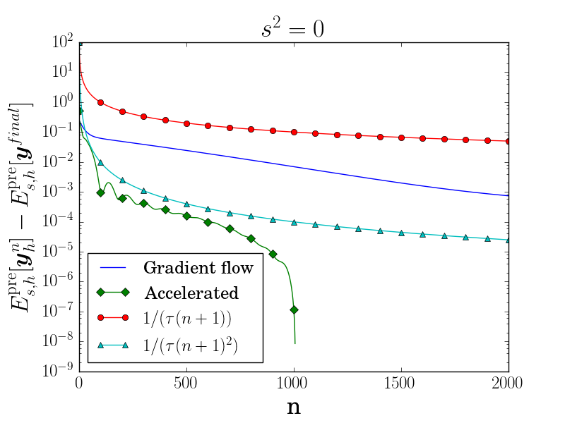
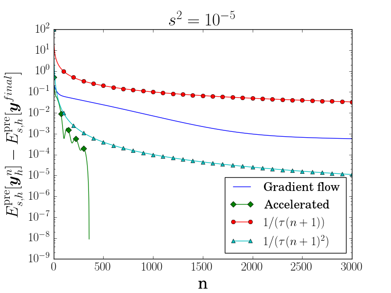
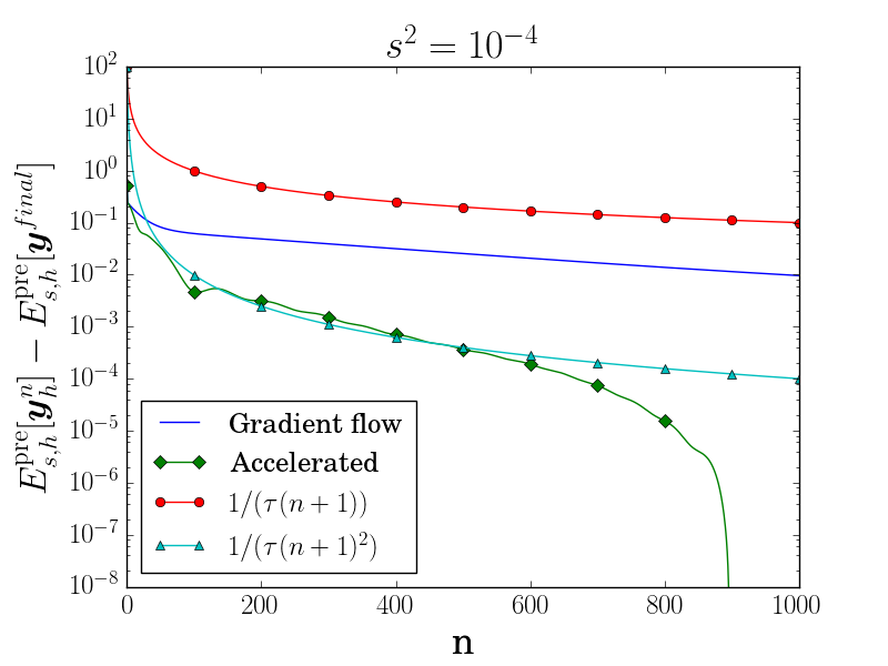
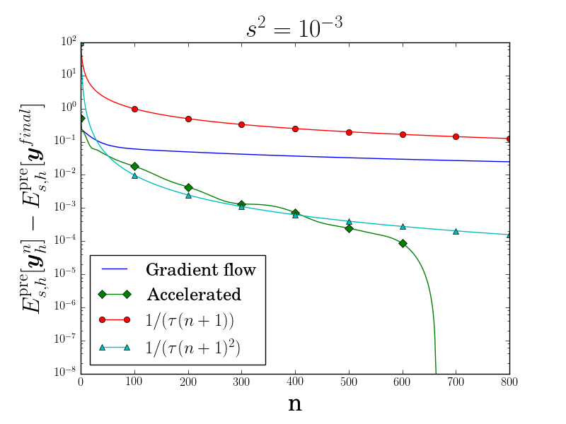
Note that the accelerating algorithm does not have the energy decreasing property that the gradient descent algorithm does. This can be observed experimentally, see Figure 4 below. However, the algorithm does appear to converge when the appropriate step size is chosen.
Finding analytic estimates for the convergence rate of the proposed algorithm remains an open problem. In Section 5.1.2 we observe at least an convergence rate and illustrate the significant gain when the accelerated version of the algorithm is used.
4.4. Dynamics: Time Discretization
Several numerical experiments presented in Section 5 are dynamical in the sense that the data (boundary conditions and external forces) vary over the time interval . The minimizers of the different energies are thus time dependent as well.
For a positive integer , we let be the physical time-step (as opposed to the pseudo-time step used in the gradient flows) and consider the points for . We assume that the elastic relaxation is faster than the time relaxation, i.e. at each time step, the thin elastic structures have minimal energies. In particular, the deformations at each time are discrete minimizers of the discrete energy defined using the input data evaluated at .
The dynamic algorithm reads:
Initialization (): Obtain using the BC preprocessing algorithm with the prescribed conditions evaluated at ; Set ;
Dynamics (): for , do
-
i)
Obtain using the BC preprocessing algorithm with the increment boundary conditions
-
ii)
Starting from , obtain using the metric preprocessing algorithm to satisfy approximately the metric constraint;
-
iii)
Starting from , obtain using the (main) gradient flow to minimize the discrete energy with the data evaluated at .
It is important to point out that the BC preprocessing procedure embedded in the dynamic algorithm above determines the increment (rather than the preprocessed deformation directly) by solving (58)-(59) with incremental boundary conditions. This is done to take advantage of the previous step and, in particular, to avoid using a costly metric preprocessing algorithm starting from scratch at each time step.
5. Numerical Experiments
In this section, we illustrate the performance of the different algorithms. All the simulations are performed with and (note that and yield the factor 1/2 for the bilayer case) and without any external force (i.e. ) except for the experiment in Section 5.3. The polynomial degree used for the approximated deformations is chosen to be , and, unless specified otherwise, we take and for the stabilization parameters. The main gradient flow ends when
for a prescribed tolerance specified for each numerical experiment below. For the metric preprocessing we stop when
for some tolerances and specified below. Finally, for the experiments in Sections 5.1 and 5.3, where the domain consists of the unit disc, we use a quadratic mapping in (35) to better approximate the domain.
5.1. Preasymptotic
We first consider two experiments using the preasymptotic model. The first experiment illustrates the effect of the thickness of the plate on the final configuration, while the second demonstrates the advantages of the Nesterov-type acceleration discussed in Section 4.3. In both experiments the computational domain is a disc of radius one, and we use for the gradient flow pseudo time-step.
5.1.1. Disc with Oscillating Boundary
Our first experiment is inspired by [42, 47], in which a hydrogel disc of negative Gaussian curvature is observed to develop more oscillations along the boundary as its thickness is reduced. The material is prestrained according to the metric
where is the Jacobian matrix for the change of variables from polar to Cartesian coordinates and is the first fundamental form of the following deformation
| (62) |
This deformation corresponds to a disk with six wrinkles.
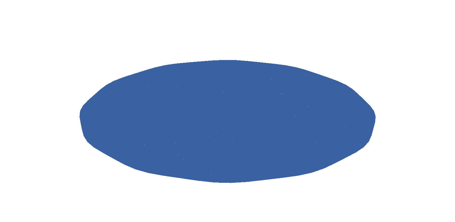
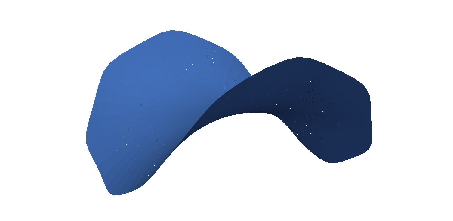
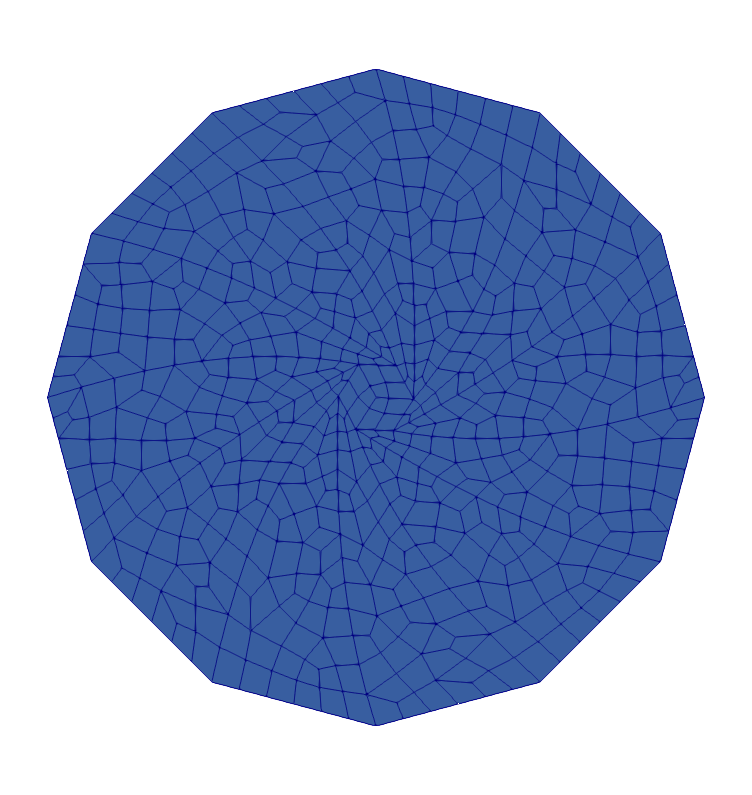
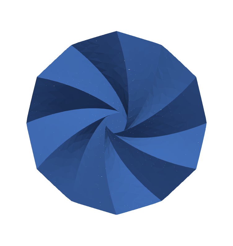
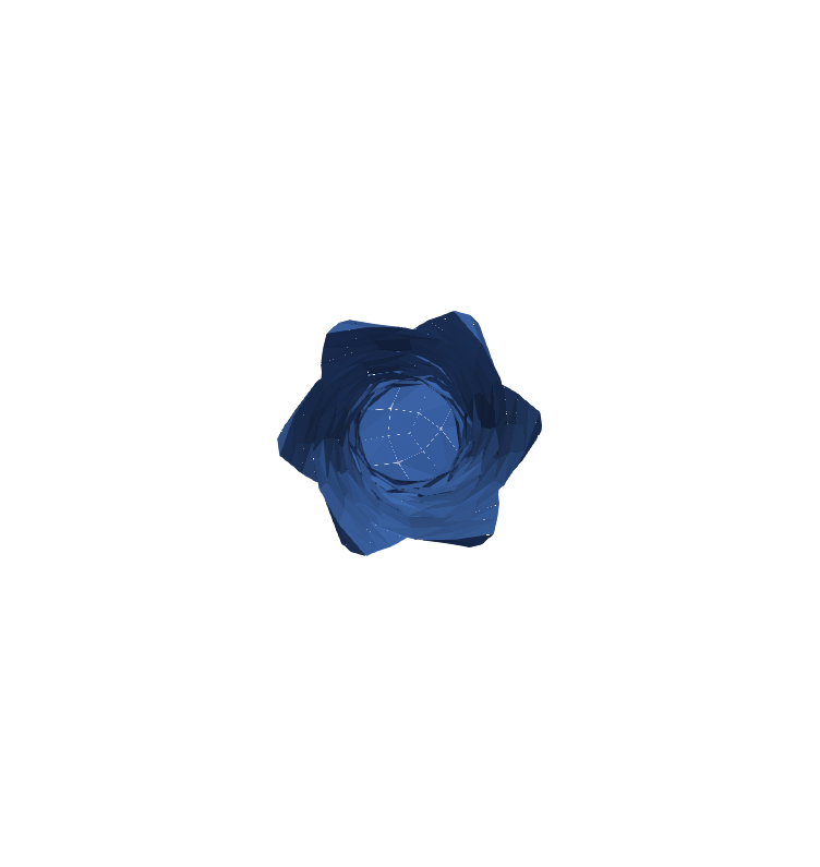
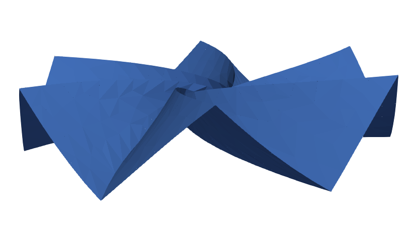
For the discretization, our subdivision consists of 1280 quadrilaterals and a total of degrees of freedom. The initial deformation is taken to be the continuous Lagrange interpolant of (62). We set for the stopping criterion and run the experiment for , , , and .
The computed deformations minimizing the preasymptotic energy are provided in Figure 3. In accordance with the laboratory experiments [42, 47], the number of wrinkles increases from 0 to 6 as decreases.
5.1.2. Accelerated Algorithm
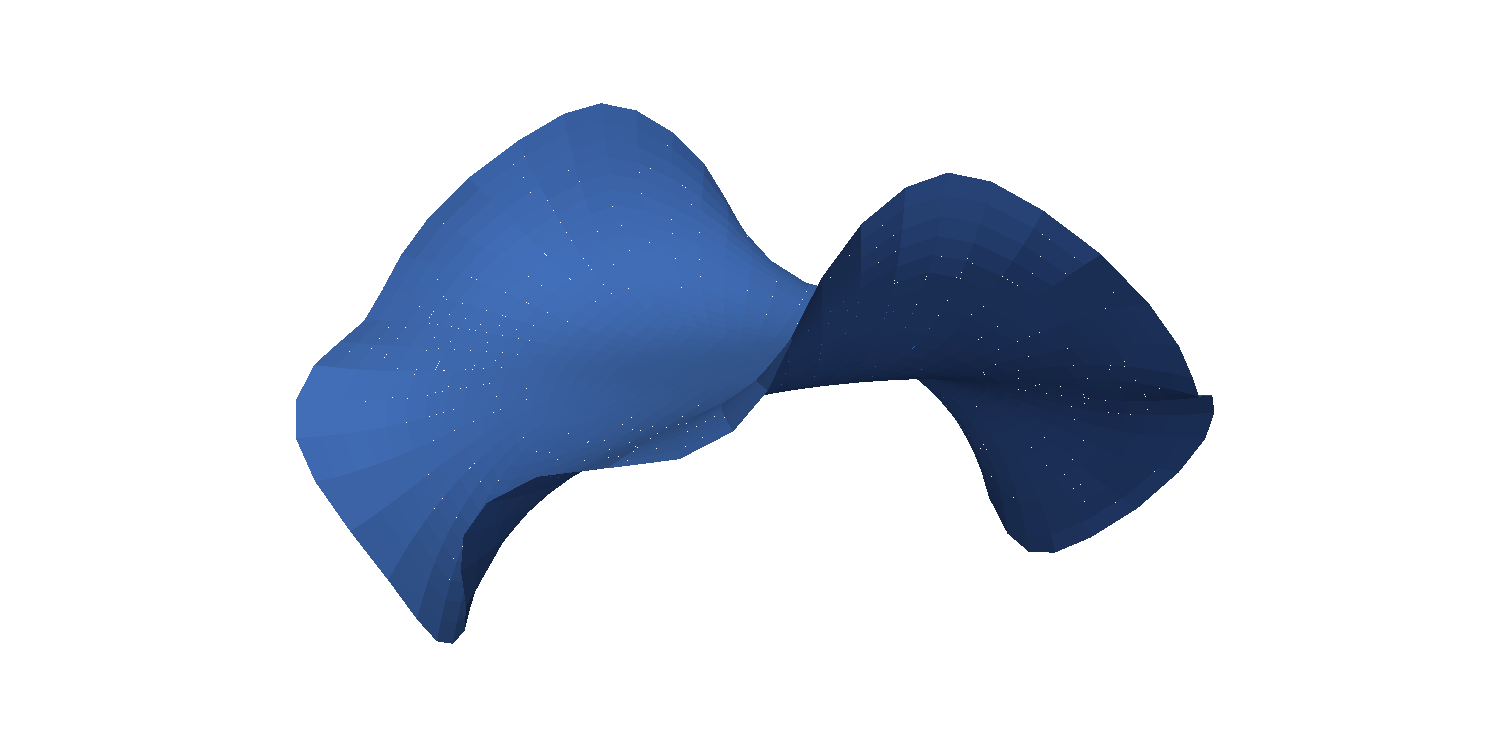
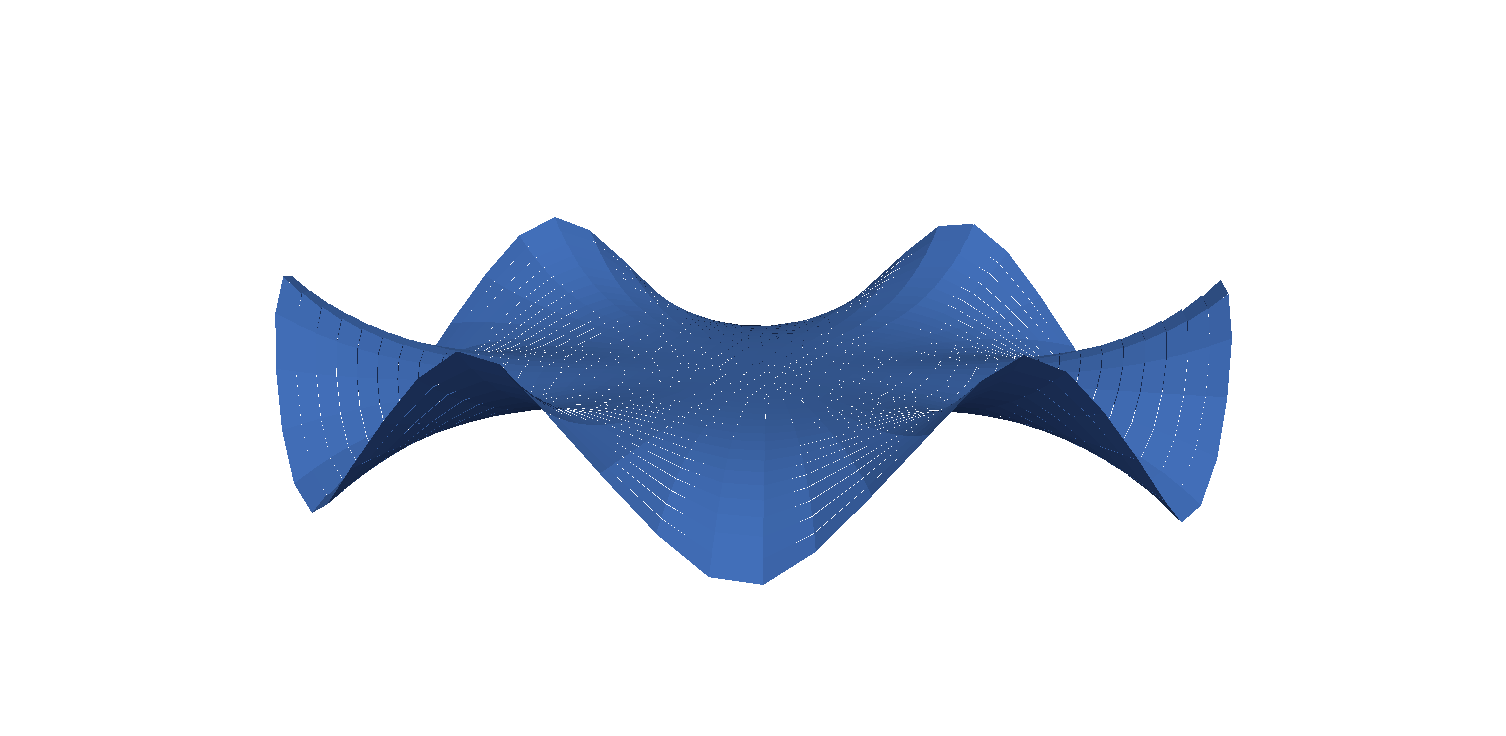
This example illustrates the benefits of using the accelerated algorithm introduced in Section 4.3 over our original gradient flow. This time the material is characterized by a “bubble” metric with positive Gaussian curvature, namely
with and .
The mesh for this experiment consists of 320 quadrilaterals and a total of degrees of freedom. The initial deformation is taken to be the continuous Lagrange interpolant of the shallow paraboloid . This gives a slight initial bending that allows the simulation to find a non-flat minimizer. (Recall from Section 4.2 that the flat configuration is a local minimizer of the preasymptotic energy.) For the thickness of the material, we use the values , , , and and we set as stopping criterion.
The discrete stretching energy and bending energy along with the number of iterations needed to reach the tolerance are reported in Table 1 when using the standard gradient flow and the accelerated algorithm. We observe that the accelerated algorithm finishes in much fewer iterations for all values of the thickness . The approximate preasymptotic energy versus the algorithm iteration number is depicted in Figure 4 for the different values of considered. When using a standard gradient flow, we observe numerically that the energy decay is like , while the accelerated algorithm exhibits a decay similar to . The latter is the expected convergence rate when using Nesterov-type accelerations.
| Discrete Gradient Flow | Accelerated Gradient Flow | |||||
|---|---|---|---|---|---|---|
| Iterations | Iterations | |||||
| 0 | 2.390e-4 | 0 | 17746 | 8.098e-6 | 0 | 1007 |
| 1.525e-4 | 2.685e-4 | 26784 | 2.694e-4 | 3.990e-4 | 359 | |
| 4.479e-5 | 5.951e-4 | 37799 | 6.350e-6 | 4.095e-4 | 896 | |
| 5.595e-5 | 2.843e-3 | 39533 | 3.920e-5 | 2.741e-3 | 664 | |
5.2. Bilayer and Folding
We consider here two experiments taken from [66], referred to as diamond and bird in the following. They illustrate the rigidity, robustness, and great variety of shapes achievable with this technology. In these examples, the computational domain consists of a collection of subdomains delimited by creases where folding is allowed. The bilayer material is designed to yield a piecewise constant spontaneous curvature tensor on each subdomain with .
In both experiments we set for the gradient flow pseudo time-step and for the stopping criterion.
5.2.1. Diamond
The diamond computational domain is provided in Figure 5 (left). It consists of the square rotated counter-clockwise by an angle of . The two dashed red curves represent the creases. They are quadratic Bézier curves with the origin as control point. The point is at distance from on the segment from to , and similarly for the three other points. We denote by the spontaneous curvature associated with each subdomain and set
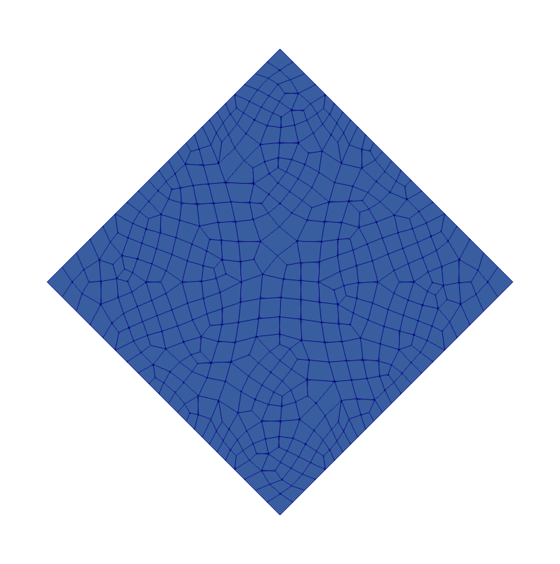
The subdivision is depicted in Figure 5 (right). It consists of quadrilaterals with maximal mesh size (total of degrees of freedom, for the deformation and for the Lagrange multipliers used to enforce the linearized isometry constraint). Moreover, the initial deformation is taken to be the identity map for which and . The deformations obtained at several steps of the gradient flow are provided in Figure 6, including the final (equilibrium) deformation reached in iterations. For the final deformation, the energy and isometry defect are and , respectively.


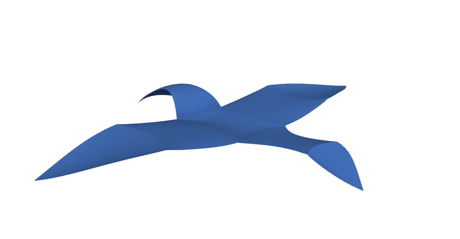
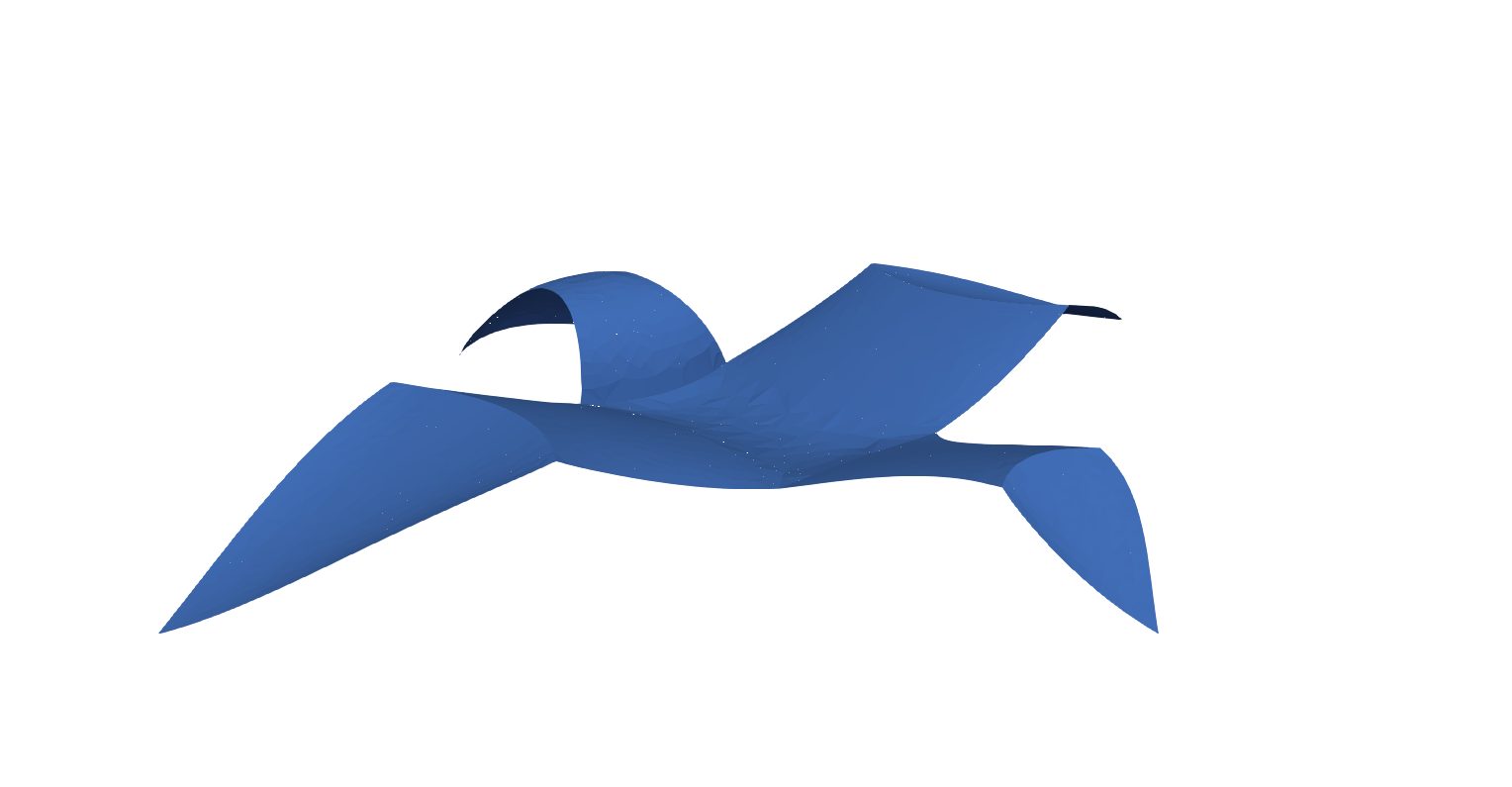
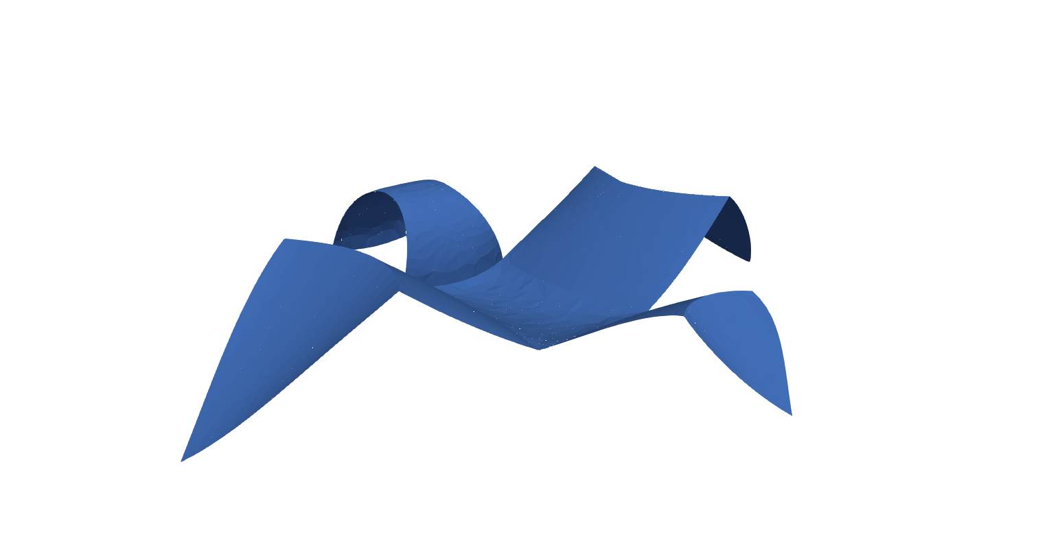
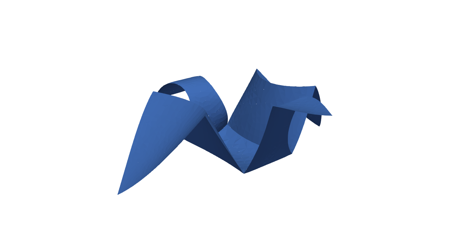
5.2.2. Bird
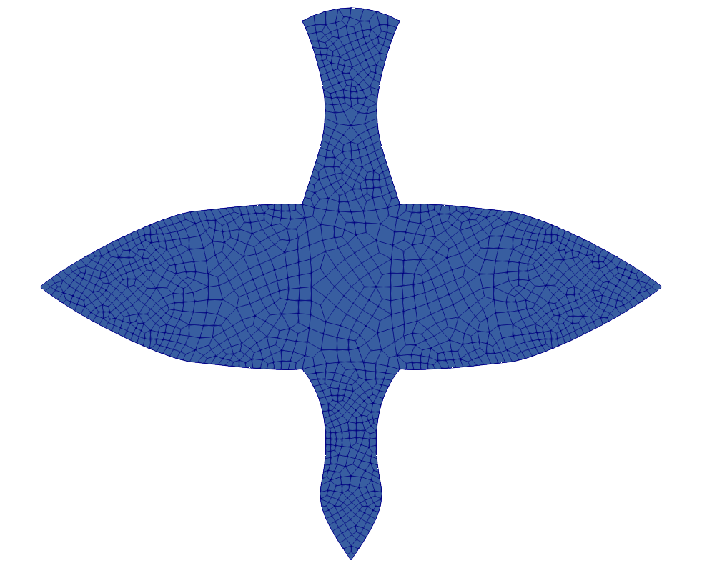
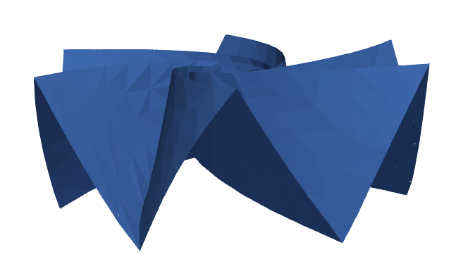
The bird geometry is depicted in Figure 7. It consists of 26 curves: 17 for the boundary of (black plain curves), 7 creases (red dashed curves), and 1 extra curve on the tail (black dotted curve) which is only used for the construction of the subdivision (i.e. no folding is possible across this curve). All the curves are quadratic or cubic Bézier curves, i.e. obtained using one or two control points. The latter are chosen so that we obtain a geometry similar to [66]. In this example, the piecewise constant spontaneous curvature tensors are given on each subdomain by
The mesh is constituted of quadrilaterals with maximal mesh size (total of degrees of freedom, for the deformation and for the Lagrange multipliers used to enforce the linearized isometry constraint), see Figure 8.
The initial deformation is again taken to be the identity map for which and . The deformation obtained after , , and (final) iterations are given in Figure 9. For the latter the energy is while the isometry defect is .
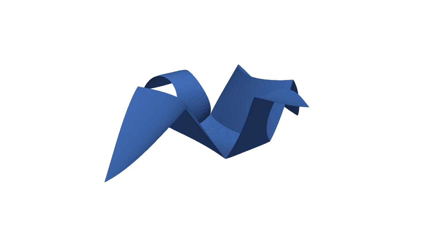
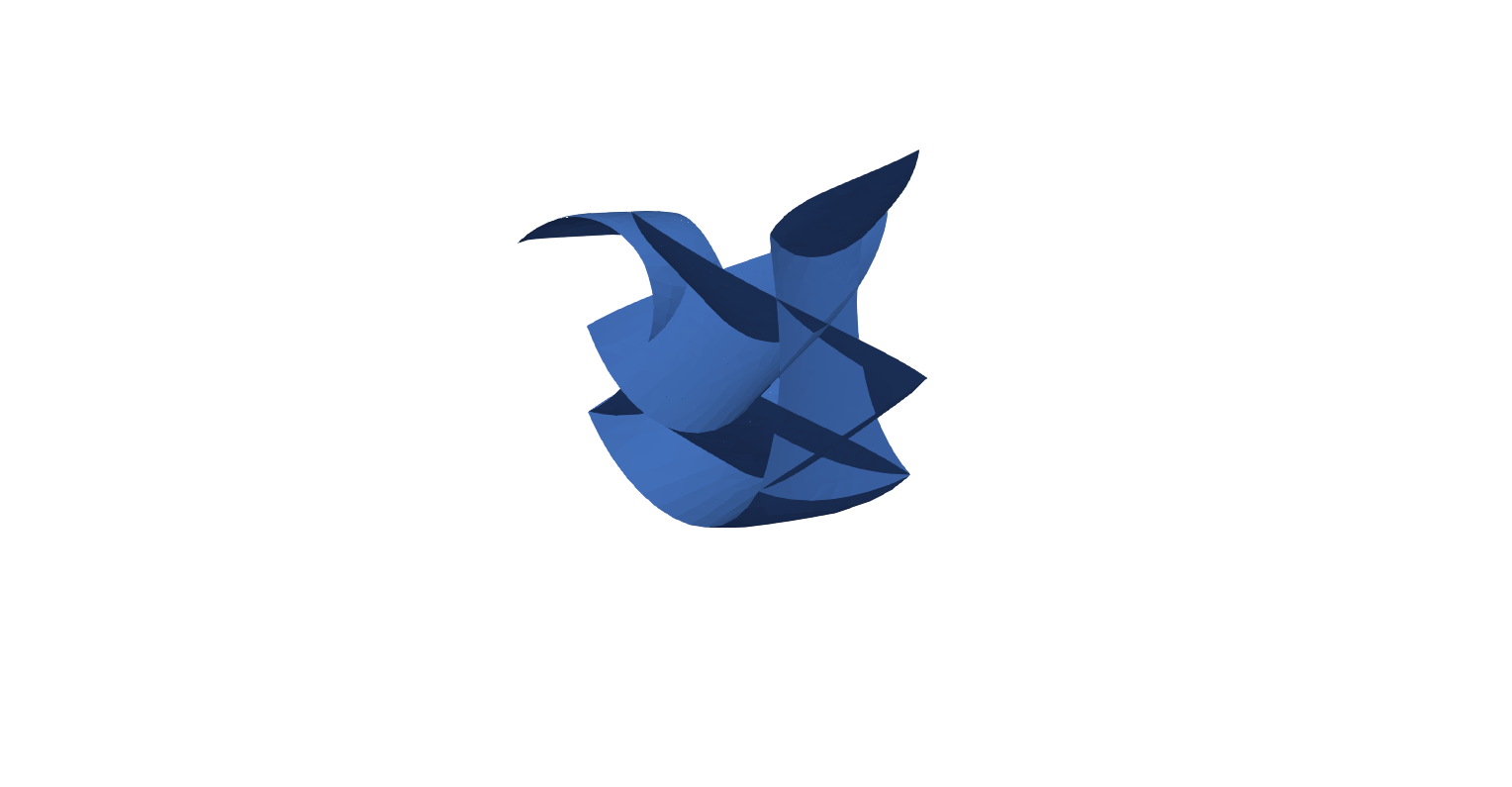
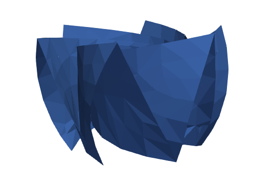
It is worth pointing out that the equilibrium shape obtained is rather sensitive to the value of the spontaneous curvature tensors. To illustrate this, a coefficient instead of in and leads to an equilibrium deformation reported in Figure 10. After iteration of the gradient flow, the deformation is similar to the one obtained in Figure 9 (bottom-right), but the final deformation reached in iterations is quite different.
5.3. Single Layer with Time-Dependent Force
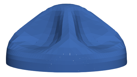
In this experiment, the domain is the unit disc endowed with a prestrain metric corresponding to a half-sphere, namely with
| (63) |
where the small parameter is introduced to avoid singularities at the boundary . We study the effect of a uniform axial force directed towards the center of the sphere. When the external force is sufficiently strong, we expect the sphere to crush like when the pressure inside a thin spherical reservoir is significantly smaller than the atmospheric pressure.
In this experiment, the external force is given by
| (64) |
where is the structure outward pointing normal and denote the time. We prescribe a mixed boundary condition with deformation given by on , which is compatible with (63).
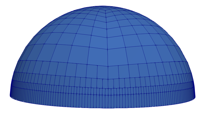
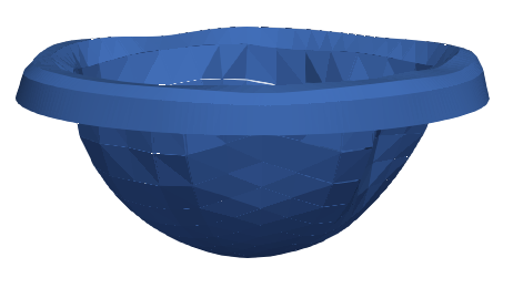
The subdivision of consists of 992 quadrilaterals with hanging nodes and of maximal mesh size (total of 29760 degrees of freedom, for the deformation and for the Lagrange multipliers used to enforce the linearized metric constraint). It is finer near the boundary where more stretching is expected. The initial deformation is taken to be the continuous Lagrange interpolant of in (63), see Figure 11, for which and . The other numerical parameters are , , and so that .
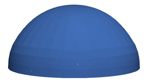
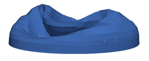
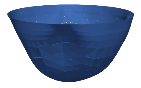
For , the equilibrium deformation is similar to the initial one given in Figure 11. The number of gradient flow iterations are 1594 for and between 8 to 101 for . When , and the object cannot sustain the corresponding force anymore. It collapses and deforms all the way to a half-sphere in the opposite direction. In particular, the range of values for the third component of the deformation is at the first iteration and at the last iteration of the gradient flow (81484). We refer to Figure 12 for the deformation obtained at different steps of the gradient flow and to Table 2 for the corresponding energy metric defect.
| 0 | 738.520 | 0.206666 |
| 400 | 711.633 | 0.245251 |
| 800 | 597.757 | 0.351605 |
| 1200 | 313.706 | 0.524551 |
| 81484 | 49.763 | 0.528641 |
5.4. Starshade Experiment
The starshade technology was developed as part of the NASA exoplanet exploration program. Starshades are occulters external to a telescope that shade the light from stars when imaging planets [55]. They fold to minimize the space they occupy when transported in rockets and are easily deployable when arrived at destination.
The mathematical model corresponds to the single layer case with isometry constraint and time-dependent boundary conditions mimicking compression (closing) and decompression (opening). The geometry is taken from [61] and consists of a dodecagon, see Figure 13.
Inside the computational domain, there are 12 cubic Bézier curves as well as 6 straight lines (hexagon) across which folding is possible. The red dashed curves correspond to valley folds while the blue ones are mountain folds. The nodes of the dodecagon are given by
with , while the nodes of the hexagon are given by
with . For the curves, we use the following control points ():
and
The first valley curve is obtained using , , and , the first mountain curve uses , , and , the second valley curve uses , , and , and so on.
For the boundary conditions, we compress the 6 valley points , . More precisely, we consider a dynamical setting by prescribing for the following time-dependent pointwise boundary condition for the deformation
| (65) |
where is a compression ratio. Using the strategy described in Section 4.4, we compute an approximate equilibrium deformation at time , . Recall that this entails running the BC preprocessing for the variation imposing the pointwise conditions
Note that at , and in particular, the BC preprocessing with the above boundary conditions results in a flat deformation which is conserved by the metric preprocessing and gradient flow. In order to generate an out of plane deformation, the boundary conditions for the initialization step (see case in Section 4.4) are modified to be (65) for the valley points and for the 6 mountain points , .
The time-step for the time discretization is , and steps are performed. The gradient flow parameters are and while , , and are chosen for the metric preprocessing. The computational domain subdivision consists of quadrilaterals of maximum mesh size (total of degrees of freedom, for the deformation and for the Lagrange multipliers used to enforce the linearized isometry constraint), see Figure 14. The penalty parameters are .
The equilibrium deformations obtained for several time are reported in Figure 15, see Figure 16 for corresponding side views.


References
- [1] Silas Alben, Bavani Balakrisnan, and Elisabeth Smela. Edge effects determine the direction of bilayer bending. Nano Lett., 11(6):2280–2285, 2011.
- [2] Douglas N. Arnold, Franco Brezzi, Bernardo Cockburn, and L. Donatella Marini. Unified analysis of discontinuous Galerkin methods for elliptic problems. SIAM J. Numer. Anal., 39(5):1749–1779, 2002.
- [3] Bavani Balakrisnan, Alek Nacev, and Elisabeth Smela. Design of bending multi-layer electroactive polymer actuators. Smart Mater. Struct., 24(4):045032, 2015.
- [4] Sören Bartels. Finite element approximation of large bending isometries. Numer. Math., 124(3):415–440, 2013.
- [5] Sören Bartels. Finite element simulation of nonlinear bending models for thin elastic rods and plates. In Handbook of Numerical Analysis, volume 21, pages 221–273. Elsevier, 2020.
- [6] Sören Bartels, Andrea Bonito, and Peter Hornung. Modeling and simulation of thin sheet folding. Interfaces Free Bound., 24(4):459–485, 2022.
- [7] Sören Bartels, Andrea Bonito, and Ricardo H. Nochetto. Bilayer plates: Model reduction, ‐convergent finite element approximation, and discrete gradient flow. Comm. Pure Appl. Math., 70(3):547–589, 2017.
- [8] Sören Bartels, Andrea Bonito, and Philipp Tscherner. Error estimates for a linear folding model. IMA J. Numer. Anal., 2023.
- [9] Sören Bartels and Christian Palus. Stable gradient flow discretizations for simulating bilayer plate bending with isometry and obstacle constraints. IMA J. Numer. Anal., 42(3):1903–1928, 2021.
- [10] Francesco Bassi and Stefano Rebay. A high-order accurate discontinuous finite element method for the numerical solution of the compressible Navier–Stokes equations. J. Comput. Phys., 131(2):267–279, 1997.
- [11] Noy Bassik, Beza Abebe, Kate Laflin, and David Gracias. Photolithographically patterned smart hydrogel based bilayer actuators. Polymer, 51(26):6093–6098, 2010.
- [12] Amir Beck and Marc Teboulle. A fast iterative shrinkage-thresholding algorithm for linear inverse problems. SIAM J. Imaging Sci., 2(1):183–202, 2009.
- [13] Peter Bella and Robert Kohn. Metric-induced wrinkling of a thin elastic sheet. J. Nonlinear Sci., 24:1147–1176, 2014.
- [14] Kaushik Bhattacharya, Marta Lewicka, and Mathia Schäffner. Plates with incompatible prestrain. Arch. Rational Mech. Anal., 221(1):143–181, 2016.
- [15] Klaus Böhnlein, Stefan Neukamm, David Padilla-Garza, and Oliver Sander. A homogenized bending theory for prestrained plates. J. Nonlinear Sci., 33(22):1–90, 2022.
- [16] Andrea Bonito, Diane Guignard, and Angelique Morvant. A note on the numerical approximation of thin structures. In preparation, 2023.
- [17] Andrea Bonito, Diane Guignard, Ricardo H. Nochetto, and Shuo Yang. LDG approximation of large deformations of prestrained plates. J. Comput. Phys., 448:110719, 2022.
- [18] Andrea Bonito, Diane Guignard, Ricardo H. Nochetto, and Shuo Yang. Numerical analysis of the LDG method for large deformations of prestrained plates. IMA J. Numer. Anal., 43:627–662, 2023.
- [19] Andrea Bonito and Ricardo H. Nochetto. Quasi-optimal convergence rate of an adaptive discontinuous Galerkin method. SIAM J. Numer. Anal., 48(2):734–771, 2010.
- [20] Andrea Bonito, Ricardo H. Nochetto, and Dimitris Ntogkas. Discontinuous Galerkin approach to large bending deformation of a bilayer plate with isometry constraint. J. Comput. Phys., 423:109785, 2020.
- [21] Andrea Bonito, Ricardo H. Nochetto, and Dimitris Ntogkas. DG approach to large bending deformations with isometry constraint. Math. Models Methods Appl. Sci., 31(01):133–175, 2021.
- [22] Andrea Bonito, Ricardo H. Nochetto, and Shuo Yang. -convergent LDG method for large bending deformations of bilayer plates. arXiv preprint arXiv:2301.03151 [math.NA], 2023.
- [23] Franco Brezzi, Gianmarco Manzini, Donatella Marini, Paola Pietra, and Alessandro Russo. Discontinuous Galerkin approximations for elliptic problems. Numer. Methods Partial Differential Equations, 16(4):365–378, 2000.
- [24] Antoine Chambolle and Charles H. Dossal. On the convergence of the iterates of “Fast Iterative Shrinkage/Thresholding algorithm”. J. Optim. Theory Appl., 166(3):25, 2015.
- [25] Camillo De Lellis and László Székelyhidi Jr. High dimensionality and -principle in PDE. Bull. Am. Math. Soc., 54:247–282, 2017.
- [26] Daniele A. Di Pietro and Alexandre Ern. Discrete functional analysis tools for discontinuous Galerkin methods with application to the incompressible Navier–Stokes equations. Math. Comp., 79(271):1303–1330, 2010.
- [27] Daniele A. Di Pietro and Alexandre Ern. Mathematical Aspects of Discontinuous Galerkin Methods. Mathématiques et Applications. Springer Berlin Heidelberg, 2011.
- [28] Efi Efrati, Eran Sharon, and Raz Kupferman. Elastic theory of unconstrained non-Euclidean plates. J. Mech. Phys. Solids, 57(4):762–775, 2009.
- [29] Yoël Forterre, Jan Skotheim, Jacques Dumais, and L. Mahadevan. How the Venus flytrap snaps. Nature, 433:421–425, 2005.
- [30] Gero Friesecke, Richard D. James, Maria G. Mora, and Stefan Müller. Derivation of nonlinear bending theory for shells from three dimensional nonlinear elasticity by Gamma-convergence. C.R. Math., 336(8):697–702, 2003.
- [31] Gero Friesecke, Richard D. James, and Stefan Müller. The föppl-von kármán plate theory as a low energy -limit of nonlinear elasticity. C.R. Math., 335(2):201–206, 2002.
- [32] Gero Friesecke, Richard D. James, and Stefan Müller. A theorem on geometric rigidity and the derivation of nonlinear plate theory from three‐dimensional elasticity. C.R. Math., 55(11):1461–1506, 2002.
- [33] Gero Friesecke, Richard D. James, and Stefan Müller. A hierarchy of plate models derived from nonlinear elasticity by Gamma-convergence. Arch. Rational Mech. Anal., 180(2):183–236, 2006.
- [34] Gero Friesecke, Stefan Müller, and Richard D. James. Rigorous derivation of nonlinear plate theory and geometric rigidity. C.R. Math., 334(2):173–178, 2002.
- [35] Alain Goriely and Martine Ben Amar. Differential growth and instability in elastic shells. Phys. Rev. Lett., 94(19):198103, 2005.
- [36] Mikhael Gromov. Partial Differential Relations, volume 13. Springer-Verlag, Berlin-Heidelberg, 1986.
- [37] Qing Han and Jia-Xing Hong. Isometric embedding of Riemannian manifolds in Euclidean spaces, volume 13. American Mathematical Soc., 2006.
- [38] Edwin Jager, Elisabeth Smela, and Olle Inganäs. Microfabricating conjugated polymer actuators. Science, 290(5496):1540–1545, 2000.
- [39] Jungwook Kim, James A. Hanna, Ryan C. Hayward, and Christian D. Santangelo. Thermally responsive rolling of thin gel strips with discrete variations in swelling. Soft Matter, 8(8):2375–2381, 2012.
- [40] Gustav Kirchhoff. über das Gleichgewicht und die Bewegung einer elastischen Scheibe. J. für Reine Angew. Math., 1850(40):51–88, 1850.
- [41] Yael Klein, Efi Efrati, and Eran Sharon. Shaping of elastic sheets by prescription of non-Euclidean metrics. Science, 315(5815):1116–1120, 2007.
- [42] Yael Klein, Shankar Venkataramani, and Eran Sharon. An experimental study of shape transitions and energy scaling in thin non-Euclidean plates. Phys. Rev. Lett., 106(11):118303–118306, 2011.
- [43] Nicolaas H. Kuiper. On -isometric imbeddings. i. Indag. Math. (Proceedings), 58:545–556, 1955.
- [44] Nicolaas H. Kuiper. On -isometric imbeddings. ii. Indag. Math. (Proceedings), 58:683–689, 1955.
- [45] Raz Kupferman and Jack P. Solomon. A Riemannian approach to reduced plate, shell, and rod theories. J. Funct. Anal., 266:2989–3039, 2014.
- [46] Hervé Le Dret and Annie Raoult. The nonlinear membrane model as a variational limit of nonlinear three-dimensional elasticity. J. Math. Pures Appl., 73:549–578, 1995.
- [47] Marta Lewicka and L. Mahadevan. Geometry, analysis, and morphogenesis: Problems and prospects. Bull. Am. Math. Soc., 59(3):331–369, 2021.
- [48] Marta Lewicka and Mohammad Reza Pakzad. Scaling laws for non-Euclidean plates and the isometric immersions of Riemannian metrics. ESAIM: Contr. Optim. C.A., 17(4):1158–1173, 2011.
- [49] Huan Liu, Paul Plucinsky, Fan Feng, and Richard D. James. Origami and materials science. Philos. Trans. Royal Soc., 379(2201):20200113, 2021.
- [50] August E.H. Love. A treatise on the mathematical theory of elasticity (2nd edition). Cambridge University Press, 1906.
- [51] Cy Maor and Asaf Shachar. On the role of curvature in the elastic energy of non-Euclidean thin bodies. J. Elast., 134:149–173, 2019.
- [52] Achim Menges and Steffen Reichert. Performative wood: Physically programming the responsive architecture of the HygroScope and HygroSkin projects. Archit. Des., 85(5):66–73, 2015.
- [53] Carl D. Modes, Kaushik Bhattacharya, and Mark Warner. Disclination-mediated thermo-optical response in nematic glass sheets. Phys. Rev. E, 81(6):060701, 2010.
- [54] Carl D. Modes, Kaushik Bhattacharya, and Mark Warner. Gaussian curvature from flat elastica sheets. Proc. Royal Soc., 467(2128):1121–1140, 2010.
- [55] NASA. Starshade technology development. https://exoplanets.nasa.gov/exep/technology/starshade/, accessed December 15, 2022.
- [56] John Nash. isometric imbeddings. Ann. Math., 60(3):383–396, 1954.
- [57] Yurii Nesterov. A method for solving the convex programming problem with convergence rate . Dokl. Akad. Nauk SSSR, 269(9):543–547, 1983.
- [58] Yurii Nesterov. Introductory Lectures on Convex Optimization: A Basic Course. Applied Optimization. Springer, 2004.
- [59] Yurii Nesterov. Lectures on convex optimization, volume 137 of Springer Optimization and Its Applications. Springer, 2018.
- [60] Joachim Nitsche. Über ein Variationsprinzip zur Lösung von Dirichlet-Problemen bei Verwendung von Teilräumen, die keinen Randbedingungen unterworfen sind. Abh. Math. Semin. Univ. Hambg., 36:9–15, 1971.
- [61] Jet Propulsion Laboratory California Institute of Technology. Space origami: Make your own starshade. https://www.jpl.nasa.gov/edu/learn/project/space-origami-make-your-own-starshade, accessed September 8, 2021.
- [62] Renate Sachse, Anna Westermeier, Max Mylo, Joey Nadasdi, Manfred Bischoff, Thomas Speck, and Simon Poppinga. Snapping mechanics of the Venus flytrap (Dionaea muscipula). Proc. Natl. Acad. Sci., 117(27):16035–16042, 2020.
- [63] Simon Schleicher, Julian Lienhard, Simon Poppinga, Thomas Speck, and Jan Knippers. A methodology for tranferring principles of plant movements to elastic systems in architecture. Comput. Aided Des., 60:105–117, 2015.
- [64] Bernd Schmidt. Minimal energy configurations of strained multi-layers. Calc. Var. Partial Differential Equations, 30(4):477–497, 2007.
- [65] Elisabeth Smela, Olle Inganäs, Qibing Pei, and Ingemar Lundström. Electrochemical muscles: Micromachining fingers and corkscrews. Adv. Mater. Lett., 5(9):630–632, 1993.
- [66] Yasaman Tahouni, Tiffany Cheng, Dylan Wood, Renate Sachse, Rebecca Thierer, Manfred Bischoff, and Achim Menges. Self-shaping curved folding: A 4D-printing method for fabrication of self-folding curved crease structures. In Symposium on Computational Fabrication, number 5 in SCF ’20, pages 1–11. Association for Computing Machinery, 2020.
- [67] Dylan Wood, Chiara Vailati, Achim Menges, and Markus Rüggeberg. Hygroscopically actuated wood elements for weather responsive and self-forming building parts - facilitating upscaling and complex shape changes. Constr. Build. Mater., 165:782–791, 2018.
- [68] Zi L. Wu, Michael Moshe, Jesse Greener, Heloise Therien-Aubin, Zhihong Nie, Eran Sharon, and Eugenia Kumacheva. Three-dimensional shape transformations of hydrogel sheets induced by small-scale modulation of internal stresses. Nat. Commun., 4:1586, 2013.
- [69] Arash Yavari. A geometric theory of growth mechanics. J. Nonlinear Sci., 20(6):781–830, 2010.