FETA: Flow-Enhanced Transportation for Anomaly Detection

Abstract

Resonant anomaly detection is a promising framework for model-independent searches for new particles. Weakly supervised resonant anomaly detection methods compare data with a potential signal against a template of the Standard Model (SM) background inferred from sideband regions. We propose a means to generate this background template that uses a flow-based model to create a mapping between high-fidelity SM simulations and the data. The flow is trained in sideband regions with the signal region blinded, and the flow is conditioned on the resonant feature (mass) such that it can be interpolated into the signal region. To illustrate this approach, we use simulated collisions from the Large Hadron Collider (LHC) Olympics Dataset. We find that our flow-constructed background method has competitive sensitivity with other recent proposals and can therefore provide complementary information to improve future searches.

I Introduction

While the Large Hadron Collider (LHC) has been operational for over a decade, no targeted search for physics beyond the Standard Model has found significant evidence for new particles or forces of nature. As a result, there has recently been a growing interest in model-agnostic searches: in such studies, the goal is to find anomalies while making few assumptions about the underlying physics model that could have produced them. This mode of analysis is highly general, and it has gained momentum from recent advances for modeling, classifying, and finding anomalies in data. For a broad review of the role of modern machine learning (ML) methods in searches for new physics, see Karagiorgi et al. (2022); for performance summaries of ML-inspired methods on LHC-like data, see the LHC Olympics Kasieczka et al. (2021) and Dark Machines Anomaly Score Challenge Aarrestad et al. (2022) reports.

One class of anomaly detection searches is for resonant anomalies. In this case, we assume that the beyond-the-Standard Model (BSM) physics signature would be resonant in at least one feature, typically some sort of mass. Such a signal might correspond to the production of a new on-shell particle. These “bump hunts” search for an excess in the mass feature above the known Standard Model (SM) background in a well-defined signal region. However, such searches require the existence of accurate SM background templates within the signal region. While particle generators for SM physics exist, the resulting simulated data (even with detector effects added) is not accurate enough to be used as a background for bump hunts in hadronic final states: hard process generators carry out perturbative calculations only to NLO, showering simulators make use of heuristic nonperturbative models, and detector simulators make necessary simplifying assumptions about particle-detector interactions in order to speed up runtime.

In response to this problem of subaccurate particle generators, a number of studies have focused on constructing SM background templates for LHC-like detected data within a signal region. Broadly, methods can be categorized on two qualities:

1. Simulation-assisted vs. data-driven. For simulation assisted methods, the background template construction is informed by a set of simulated LHC-like collider data representing SM processes; for data-driven methods, data from sidebands mass regions is used, where the sidebands are far enough from the resonant process such that the data can be treated as a proxy for SM background.

2. Likelihood learning vs. feature morphing. For the former, methods learn the likelihood of a SM-only dataset (such as simulation, or detected data in sidebands) where there are no signal events. This learned likelihood is then interpolated into the signal region to act as a SM background template above which signal events might be detected. Alternatively, methods can physically morph features from the SM-only dataset to the detected, signal-containing dataset.

A number of previous methods for SM background construction are classified visually in Table 1. This two-axis scheme is not meant to be all-encompassing, as there exist many methods for anomaly detection that cannot be so neatly classified (see Benkendorfer et al. (2021); Amram and Suarez (2021); Choi et al. (2020); CMS (2022) for examples of such methods in practice).

	Simulation-assisted	Data-driven
Likelihood learning	Salad Andreassen et al. (2020)	Overdensity searches Stein et al. (2020), Anode Nachman and Shih (2020), (La)Cathode Hallin et al. (2022a, b)
Feature morphing	Feta (this work)	Curtains Raine et al. (2022)

Table 1: Broadly speaking, many methods for constructing SM background templates for resonant anomaly detection can be classified on two axes. In this study, we introduce the Feta method.

In this paper, we propose the “Flow-Enhanced Transportation for Anomaly Detection” (Feta) method to model SM-like background at the LHC. Feta is simulation-assisted and relies on feature morphing, therefore filling the previously empty section of Table 1.

In Feta, we train a normalizing flow Tabak and Turner (2013) to learn a mapping between simulation and data in sidebands regions. We then apply the learned mapping to signal region simulation to create a simulation-informed template for signal region SM background. Feta benefits from being simulation-assisted since it can use simulated SM data as a physically-informed prior for the background template; the method further benefits from using feature morphing since it is robust to mapping between feature spaces with non-overlapping support.

The structure of this paper is as follows. In Sec. II, we provide a concise background of normalizing flows and outline how they will be applied to physics-specific datasets. In Sec. III, we illustrate the effectiveness of flow-based models for creating context-dependent mappings with a toy example of triangular datasets. In Sec. IV, we exchange the toy models for LHC-like data and use Feta to create a model for LHC-like detected SM data. In Sec. V, we test the performance of Feta in a series of realistic anomaly detection tasks. In Sec. VI, we conclude and suggest avenues for further study.

II Methodology

II.1 Normalizing flows as morphing functions

Normalizing flows are constructed from invertible neural networks between sets of variables sampled from different probability densities. Given a random variable $X$ sampled from a reference distribution $p_{R}$, one can define a transformation $T$ that produces another random variable $Z$, i.e. $Z=T(X)$. The density of $Z$ is then given by $p_{Z}(Z)=p_{R}(X)|\textrm{det}\frac{\partial T}{\partial X}|^{-1}$. By chaining together a number of transformations $T_{i}$, one can produce an arbitrarily complex mapping between the initial reference density $p_{R}$ and a target distribution $p_{T}$. Typically, the target density is taken to be a standard normal distribution. (Hence the name “normalizing” flow.)

In this work, we use the normalizing flow both for its density estimation power and its ability to construct morphing functions between nontrivial reference $X_{R}\sim p_{R}$ and target $X_{T}\sim p_{T}$ distributions. Our reference density is derived from Standard Model simulation ($X_{\mathrm{SIM}}\sim p_{\mathrm{SIM}}$), and our target dataset is derived from detected data ($X_{\mathrm{DAT}}\sim p_{\mathrm{DAT}}$).

More explicitly, we define a set of $N$ event observables such that events in the reference and target are $N$-dimensional vectors $X_{\mathrm{SIM}}$ and $X_{\mathrm{DAT}}$, which respectively are sampled from the $N$-dimensional feature densities $p_{\mathrm{SIM}}$ and $p_{\mathrm{DAT}}$. We then train a flow to learn the mapping $T$ between $p_{\mathrm{SIM}}$ and $p_{\mathrm{DAT}}$. In training the flow, we must ensure that the learned mapping is between simulated Standard-Model background and LHC-detected background. For resonant anomalies, we assume that the signal will be localized in one feature $m_{res}$. This allows us to define sidebands (SB) and a signal region (SR) in $m_{res}$, where data from the former regions is assumed to follow the SM distribution. We then train the flow only on data from SB, using the resonant feature to condition the mapping $T(\cdot|m_{res})$. The learned flow is then applied to simulation in the SR to produce an approximation of $X_{\textrm{DAT}}$: $X^{*}_{\textrm{SIM}}=T(X_{\textrm{SIM}}|m_{res})$ for LHC-detected background in the SR. A schematic of this method is shown in Fig. 1.

Figure 1: A schematic of the Feta method. We train a flow to learn the mapping between simulation and data in sidebands regions, which are expected to be background-only. We then apply the learned flow to simulation in a signal region to produce an approximation for background in that region.

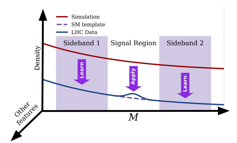
There are several advantages to using a flow-based architecture over other architectures such as GANs or VAEs. Normalizing flows are known to be more stable and achieve convergence during training faster, especially in higher dimensions. This property allows for the freedom to choose a larger feature space $X$, which may be desirable for a model-agnostic study. For GANs specifically, attempting to learn conditional mappings between datasets is not an easily done task. In addition, the density estimating power of the normalizing flow allows us to oversample from the reference distribution and reduce statistical uncertainties (explored in more detail in App. A). This is not possible with VAEs, which require the definition of explicit pairs to train the encoder-decoder architecture.

II.2 Flow construction

All flows were constructed using the nflows package Durkan et al. (2020) and were trained using PyTorch Paszke et al. (2019).

As an important procedural note: to learn a flow that maps between two nontrivial densities, we use a two-step procedure. We first train a Base Density normalizing flow to learn the mapping between a normal distribution and the reference density $p_{R}$ across all mass bands (i.e. using reference data from both the SB and SR). We then train a Transport flow to learn the mapping between the Base Density distribution and the target density $p_{T}$, this time only using data from the SB. This specific method, which allows for the use of flows to map between nontrivial distributions, was proposed and implemented in the Curtains background construction method (and is further explored in Klein et al. (2022)). It is thus more accurate to simply call Feta a flow-based method, rather than a normalizing flow-based one.

III Testing the Feta method with a toy model

To concretely illustrate the Feta method, we train a flow to map between two toy triangular datasets. Both datasets contain 100,000 samples in a two-dimensional feature space, with a feature $X$ that is conditionally dependent on a feature $M$. This conditioning feature can be interpreted as a mass-like feature, or one in which we expect an anomaly to be resonant.

III.1 Toy model datasets

To construct each dataset, we first generate samples of the conditioning (resonant) feature $M$, which we take to be uniformly distributed between (0, 1). On this feature, we define the signal region SR $\sim$ (0.34, 0.66). We also define two sidebands, SB1 $\sim$ (0.0, 0.34) on the low mass side of the SR, and SB2 $\sim$ (0.66, 1.0) on the high mass side.

For the corresponding nonresonant feature, we draw samples from a triangular dataset with endpoints at (0, 1). In order to condition this feature $X$ on the mass, for each sample we define the midpoints $m_{R}$, $m_{T}$ of the triangular distributions for reference and target to be linear functions of $M$, $m_{\textrm{R}}=0.4995M$ and $m_{\textrm{T}}=0.4995M+0.5005$. Then the toy reference dataset $X_{R}$ consists of left-triangular dataset samples in the range (0, 1), and the toy target dataset $X_{T}$ consists of right-triangular samples. We further shift all the samples $X_{T}$ of the target dataset by 0.5 such that the reference and the target sets have nonidentical support. Samples from the two datasets are shown in Fig. 2.

Figure 2: Toy datasets $X_{\textrm{R}}$ and $X_{\textrm{T}}$. The feature $X$ is a function of the conditioning feature $M$.

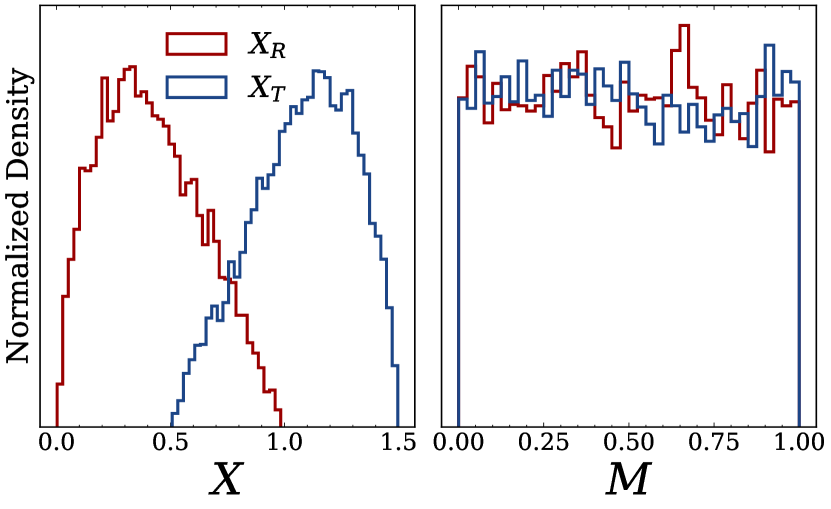
The flow architecture and hyperparameters are given in Table 2. All settings were optimized via manual tuning and were chosen to give the best possible performance on the SB regions (as quantified by the ROC AUC, which is defined in Sec. III.2). Flow training is optimized with AdamW Kingma and Ba (2014), and the learning rate is annealed to zero following a cosine schedule Loshchilov and Hutter (2016). Before training, all features are minmaxscaled to the range (-3, 3), which was found to be optimal with respect to the flow training; further, the samples are split into training (80%) and validation (20%) sets. The model from the epoch with the lowest validation loss is used for evaluation.

Parameter	Base density flow	Transport flow
Flow type	Autoregressive Huang et al. (2018)	Coupling
Spline	Piecewise RQ	Piecewise RQ
Num. MADE blocks	8	8
Num. layers	2	2
Num. hidden features	16	16
Epochs	20	20
Batch size	128	256
Learning rate	3$\times 10^{-4}$	3$\times 10^{-4}$
Weight Decay	1$\times 10^{-4}$	1$\times 10^{-5}$

Table 2: (RQ = rational quadratic; MADE = Masked Autoencoder for Distribution Estimation Germain et al. (2015).) Flow architecture and training hyperparameters used for the toy (triangular) dataset. Both the Base Density and Transport flow parameters were optimized through manual tuning.

III.2 Toy model results

Plots of the reference $X_{R}$, transformed reference $X^{*}_{R}$ as found by the Feta method, and target $X_{T}$ distributions are shown in Fig. 3. We compare the distributions separately in SB1, SR, and SB2 (recall that the flow is trained only on data from SB1 and SB2 and is applied to the blinded SR data). Qualitatively, there is excellent agreement between the distributions for $X^{*}_{R}$ and $X_{T}$ in SB1 and SB2 and good agreement in the SR. We conclude that the flow has learned to map between the reference and the target data.

In Fig. 3, we also plot the reweighted reference $X^{W}_{R}$ as found through the Salad method. For this method, we train a binary classifier to discriminate between $X_{R}$ and $X_{T}$. Such a classifier will learn the likelihood ratio between the reference and the target distributions. This likelihood ratio can then be interpolated into the SR and used to reweight $X_{R}$. Note that for this toy model, feature reweighting is expected to fail due to the fact that there are regions of non-overlapping support between the reference and target.

Figure 3: Probability distributions for $X_{R}$, $X^{*}_{R}$, and $X_{T}$ for the toy model. The $X^{*}_{R}$ samples represent the trained flow acting upon $X_{R}$. The good agreement between $X^{*}_{R}$ and $X_{T}$ indicates that the flow has successfully learned to map between the two datasets. We also provide the distribution for reweighted reference $X^{W}_{R}$ to illustrate its failure to provide an accurate model for $X_{T}$, as the reference and target datasets have different regions of support.

We can quantify the performance of the learned morphing function by training a 5-fold binary classifier neural network to discriminate between $X^{*}_{R}$ and $X_{T}$. Each classifier is a fully connected (dense) network, with linear layers of sizes (5, 64, 32, 1) and a dropout of 0.1 between each layer. Each classifier is trained for up to 100 epochs with a batch size of 128, learning rate of 10^-3, and patience of 5 epochs. We evaluate all test data on the classifier from the fold with the best (lowest) validation loss.

As our scoring metric, we use the area under the receiver operating characteristic (ROC) curve. These AUC scores for this classifier are shown in Table 3. An ideal morphing function would result in the transformed reference and target datasets being indistinguishable from each other, which would correspond to a AUC close to 0.50. Indeed, the AUCs hit this performance benchmark, and they are also far lower than those for a classifier trained to discriminate between untransformed $X_{R}$ and $X_{T}$.

Band	AUC for $X^{*}_{R}$ vs $X_{T}$	AUC for $X_{R}$ vs $X_{T}$
SB1	0.5144 $\pm$ 0.0095	0.9830 $\pm$ 0.0009
SR	0.5117 $\pm$ 0.0040	0.9806 $\pm$ 0.0000
SB2	0.5086 $\pm$ 0.0082	0.9813 $\pm$ 0.0009

Table 3: ROC AUCs for a binary classifier trained to discriminate the transformed reference $X^{*}_{R}$ from the target dataset $X_{T}$. For comparison, we also provide the AUCs for a binary classifier trained to discriminate the untransformed reference $X_{R}$ from the target. Uncertainties are the 1$\sigma$ bounds from retraining the binary classifier 20 times, each with a different random seed.

IV Applying Feta to LHC-like data

We now move to a realistic example: training a flow to learn the morphing function between Standard Model simulation and detected data. For an ideal application of Feta, the reference dataset would consist of simulated Standard Model-like data ($X_{R}$ = $X_{\mathrm{SIM}}$), and the target dataset would consist of LHC-detected Standard Model data $X_{T}$ = $X_{\mathrm{DAT}}$). However, we do not have access to LHC data. Therefore in this study we use two distinct sets of simulated data for the reference and target datasets.

IV.1 LHCO datasets

We focus on the LHC 2020 Olympics R&D dataset Kasieczka et al. (2019, 2021). The full dataset consists of 1,000,000 background dijet events (Standard Model Quantum Chromodynamic (QCD) dijets) and 100,000 signal dijet events. The signal comes from the process $Z^{\prime}\rightarrow X(\rightarrow q\overline{q})Y(\rightarrow q\overline{q})$, with three new resonances $Z^{\prime}$ ($3.5$ TeV), $X$ (500 GeV), and $Y$ (100 GeV). Events are required to have at least one large-radius jet ($R=1$) trigger with a $p_{T}$ threshold of $1.2$ TeV. The events are generated with Herwig++Bähr et al. (2008), Pythia 8.219 Sjostrand et al. (2006); Sjöstrand et al. (2015), and Delphes 3.4.1 de Favereau et al. (2014). Each event contains up to 700 particles with three degrees of freedom (DoF) $p_{T}$, $\eta$, $\phi$.

For this study, we choose a feature space of six dijet observables $m_{J_{1}}$, $\Delta m_{JJ}$, $\tau^{21}_{J_{1}}$, $\tau^{21}_{J_{2}}$, $\Delta R_{JJ}$, and $m_{JJ}$. Following the example of the Curtains analysis, we include the $\Delta R_{JJ}$ dijet observable as a feature that is highly correlated with $m_{JJ}$.

As with many anomaly detection searches, we assume that the anomaly is resonant in one feature, $m_{JJ}$. This would correspond to a new resonant particle that would produce the two jets. The assumption of resonance allows us to define a signal region (SR) in $m_{JJ}$-space, as well as two sidebands (SB1 and SB2) on the low- and high-mass ends of the SR. The region edges are defined in Table 4. While we have chosen to focus on one SR / SB setup, one could in practice perform a sliding bump hunt and scan the SR across a wide range of resonant masses.

Band	GeV Bounds	Herwig++ events	Pythia events
SB1	(2900, 3300)	210767	212115
SR	(3300, 3700)	121978	121339
SB2	(3700, 4100)	68609	66646
SB1 $\cup$ SB2	–	279376	278761

Table 4: Band edge definitions in $m_{JJ}$-space for the LHC Olympics datasets and corresponding event counts.

The LHC Olympics dataset does not contain any LHC-detected data that would be the obvious choice for $X_{\mathrm{SIM}}$. Therefore we take the LHC Olympics Herwig++ data as our simulation dataset $X_{\mathrm{SIM}}$ and the Pythia data as our target dataset $X_{\mathrm{DAT}}$. Histograms of the six dijet observables for $X_{\mathrm{SIM}}$ and $X_{\mathrm{DAT}}$ are shown in Fig. 4.

Figure 4: Feature distributions for the six dijet observables used in the LHC Olympics analysis. SIM represents Herwig++ simulation, and DAT represents Pythia simulation. The last feature, $m_{JJ}$, is the feature in which we expect the anomaly to be resonant and conditions the flow mapping.

IV.2 Training Method

The method for training a flow on the LHC data is the same as for the toy dataset. However, the flow architectures used for LHC-like data are significantly more expressive. Architectures and hyperparameters are outlined in Table 5. Notably, the Base Density flow parameters were derived from the main architecture from Cathode (which relies on faithful density estimation of detected collider data in SB), and they were confirmed to give the best performance through manual tuning. Data is minmaxscaled to the range (-3, 3) before flow training, and a training-validation split of 80%-20% is used. All settings were manually optimized to give the best-performing flow possible, as quantified by the ROC AUCs in SB1 and SB2.

Parameter	Base Density flow	Transport flow
Flow type	Autoregressive	Coupling
Spline	Piecewise RQ	Piecewise RQ
Num. MADE blocks	15	8
Num. layers	1	2
Num. hidden features	128	32
Epochs	100	50
Batch size	128	256
Learning rate	1$\times 10^{-4}$	5$\times 10^{-4}$
Weight Decay	1$\times 10^{-4}$	1$\times 10^{-5}$

Table 5: Flow architecture and training hyperparameters used for SM background construction for the LHC Olympics dataset. The Base Density flow parameters were derived from the main architecture from Cathode, but were confirmed to give the best performance through manual tuning. The Transport flow parameters were optimized through manual tuning.

IV.3 LHCO results

In Figs. 5(a) and 5(b), we plot the distributions for $X_{\textrm{SIM}}$, $X^{*}_{\textrm{SIM}}$, and $X_{\textrm{DAT}}$ for the LHC-like data in SB1 and SB2. For each band, we also plot the ratio of untransformed and transformed simulation distributions to the target distribution. For all features, the transformed simulation $X^{*}_{\textrm{SIM}}$ is visually much closer to the target $X_{\textrm{DAT}}$ than the untransformed simulation.

(a) SB1 (low-mass sideband) distributions

(b) SB2 (high-mass sideband) distributions

(c) SR (signal region) distributions. Note that the flow was not explicitly been trained to map from $X_{\mathrm{SIM}}$ to $X_{\mathrm{DAT}}$ in this mass band, but was interpolated after training on SB1 and SB2.

Figure 5: Probability distributions and ratios for $X_{\mathrm{SIM}}$, $X^{*}_{\mathrm{SIM}}$, and $X_{\mathrm{DAT}}$ for the LHC Olympics model. The $X^{*}_{\mathrm{SIM}}$ samples represent the data that results from the trained flow acting upon $X_{\mathrm{SIM}}$. The good agreement between $X^{*}_{\mathrm{SIM}}$ and $X_{\mathrm{DAT}}$ indicates that the flow has successfully learned to map between the two datasets.

In Fig. 5(c), we provide the same distributions for $X_{\textrm{SIM}}$, $X^{*}_{\textrm{SIM}}$, and $X_{\textrm{DAT}}$ in SR. For these plots, we once again see good qualitative agreement between $X^{*}_{\textrm{SIM}}$ and $X_{\textrm{DAT}}$, despite the fact that the flow was not explicitly trained to morph between SR datasets.

In Table 6, we quantify the performance of the flow through the ROC AUC of a binary classifier (with the same architecture as in Sec. III.2) trained to discriminate $X^{*}_{\textrm{SIM}}$ from $X_{\textrm{DAT}}$ in each band. In all bands, the AUC is consistent with below 0.51, so our benchmark for indistinguishability of transformed simulation from the target is achieved.

Band	AUC for $X^{*}_{\textrm{SIM}}$ vs $X_{\textrm{DAT}}$	AUC for $X_{\textrm{SIM}}$ vs $X_{\textrm{DAT}}$
SB1	0.5128 $\pm$ 0.0032	0.5970 $\pm$ 0.0022
SR	0.5034 $\pm$ 0.0010	0.5706 $\pm$ 0.0006
SB2	0.5153 $\pm$ 0.0054	0.5938 $\pm$ 0.0031

Table 6: ROC AUCs for a binary classifier trained to discriminate the transformed simulation $X^{*}_{\textrm{SIM}}$ from the target dataset $X_{\textrm{DAT}}$. For comparison, we also provide the AUCs for a binary classifier trained to discriminate the untransformed simulation $X_{\textrm{SIM}}$ from the target.

V Using Feta for anomaly detection

For a well-trained flow, $X^{*}_{\textrm{SIM}}$ should faithfully model the SM background as would be detected at the LHC. However, if the LHC-detected data did contain some anomalous events, this would cause $X^{*}_{\textrm{SIM}}$ to differ from $X_{\textrm{DAT}}$. In this case, an avenue for resonant anomaly detection emerges. We can train a binary classifier to discriminate $X^{*}_{\textrm{SIM}}$ in the SR from data in the SR, and a significant deviation found between the distributions might provide evidence of anomalous events in the detected data. This method for anomaly detection relies on the fact that a binary classifier trained to discriminate between two mixed samples (such as a background-only SM template and a detected mixture of SM background and resonant signal) is in fact the optimal classifier for distinguishing pure signal from pure background Metodiev et al. (2017); Collins et al. (2019, 2018).

V.1 Signal injection procedure

To explore the capability of Feta for anomaly detection, we repeat the flow training method as outlined in Sec. IV.2. We inject a known number of signal events into the $X_{\textrm{DAT}}$ (Pythia) dataset. Since our chosen SR extends across the $m_{JJ}$ range [3300, 3700] GeV, this allows for possible detection of the $Z^{\prime}$ resonance centered at 3500 GeV. We test a range of signal injections, scanning over $n_{S}\in[300,500,750,1000,1200,1500,2000,2500,3000]$ (corresponding to $S/B\approx[0.30\%,\allowbreak 0.49\%,\allowbreak 0.74\%,\allowbreak 0.99\%,\allowbreak 1.18\%,1.48\%,\allowbreak 1.97\%,2.47\%,2.96\%]$). As a word of caution: despite the relatively wide SR window chosen, about 20% of the injected events go into the SB regions.

For each signal injection, we rerun the full Feta pipeline and train a flow to learn the mapping between simulation and data with the injected signal. (This retraining is necessary due to the signal contamination in the sidebands.) We then train a binary classifier (with the same architecture as in Sec. III.2) to discriminate transformed simulation from data.

We compare the results of the Feta method with those from the Cathode, Curtains, and Salad methods. For each alternative method, we use the architecture cited in the respective paper. To place all methods on an equal footing, we use the same set of training and validation dijet events for all methods. Such event breakdowns are given in Table 7. Note that all methods use the validation loss to select the best-performing model to be used for further analysis. The Feta, Cathode, and Curtains methods all make use of oversampling of the SM background template to achieve better performance, which is a mechanism that allows for the reduction of statistical uncertainties. We investigate the effects of oversampling on the Feta method performance in App. A.

Method	Train	Validation (Model Selection)	Template Samples (Evaluation)	Oversampling Factor
Feta	224k SB simulation 186k SB data	56k SB simulation 47k SB data	720k SR	$\times$6
Cathode	186k SB data	47k SB data	400k SR	$\times$3
Curtains	186k SB data	47k SB data	1120k SR	$\times$4
Salad	224k SB simulation 186k SB data	56k SB simulation 47k SB data	120k SR	N/A

Table 7: Number of dijet events used in training and validation, as well as number of events taken as the SR background template for each SM background template construction method. For the Curtains method, SR template samples are generated from transporting both the training and the validation SB samples into the SR. Note that oversampling (the reduction of statistical uncertainties by drawing more SM samples) is not possible with the Salad method, which does not use a generative model for the reference dataset. The oversampling factor is the number of SM background template samples generated over the number of dijet events used to construct the SM background template samples.

(a) Significant improvement characteristic (SIC)

(b) Rejection

(c) SIC against rejection

Figure 6: Various performance metrics for a binary classifier trained to discriminate a constructed SM background template from detected SR data. We retrain the binary classifier 20 times, each with a different random seed. Curves illustrate the median of these classifier runs, and bands represent the spread across the (16, 84) percentiles. “Full. Sup.” corresponds to a fully supervised classifier trained on pure signal and pure background.

All methods are evaluated by training a binary classifier to discriminate the SM background template samples from a set of 100k dijet data events from the SR. All classifiers are tested on the same set of 20k signal and 20k background SR dijet events, which were not used at any point during the training or validation procedures.

V.2 Anomaly detection performance summary

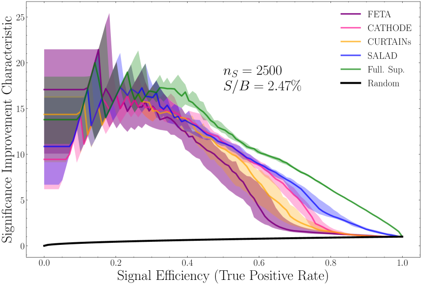
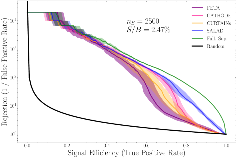
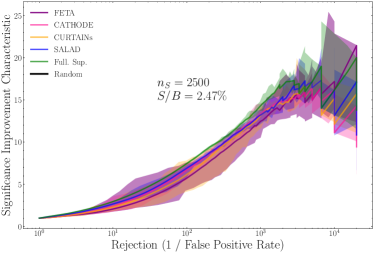
In Fig. 6, we show a selection of summary plots from this final binary classifier corresponding to 2500 injected signal events ($S/B=1.97\%$, $S/\sqrt{B}\approx 7.9$). Each curve represents the mean performance of 20 different random classifiers trained to discriminate the given SM background template from the “detected” events in the SR. Errorbands represent the spread across the (16, 84) percentiles across these 20 runs. Note that the errorbands are comparable for Feta, Cathode, Curtains, and Salad.

In Fig. 6(a), we provide the significance improvement characteristic curves, given by SIC = $\frac{\textrm{true positive rate}}{\sqrt{\textrm{false positive rate}}}$. The SIC can be interpreted in the limit of large $S$ and $B$ as the gain in signal significance (i.e. the multiplicative factor) over the initial significance that can be achieved by making a well-motivated cut on the dataset. Therefore for an optimally performing classifier, we expect to see the SIC $>>1$. In Fig. 6(b), we provide the classifier rejection curves, given by the reciprocal of the false positive rate. An optimally performing classifier should see this rejection also be $>>1$. Finally, in Fig. 6(c), we plot the SIC curves against the rejection curves.

In addition to the curves for the four methods considered, we also provide the curves corresponding to a fully supervised classifier, i.e. a classifier trained on perfectly labeled signal and background events. This curve demonstrates the maximum possible performance to discriminate SM physics from anomalous physics. Importantly, the fully supervised classifier should not be interpreted as the limiting case of an idealized anomaly detection study, which would come from a classifier trained to discriminate detected data from perfectly simulated background.

We find that the Feta method is competitive with the performance of a fully supervised classifier at signal efficiencies of around 0.3 and lower. This performance is encouraging as in practice, we would expect Feta to be used primarily in this range (for higher signal-efficiencies, the amount of background is sufficiently large that non-fully-supervised methods are unlikely to effectively find the signal). Indeed, the performance curves of Feta for all three metrics, (SIC, rejection, and SIC vs. rejection) very closely align with those of Cathode, which was demonstrated to be state-of-the-art, and Curtains.

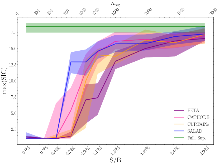
In Fig. 7, for each signal injection, we plot the maximum of the SIC, where the maximum is taken across all signal efficiencies. Since the SIC relates to an increase in signal significance from a well-motivated cut, the max(SIC) is then the best possible cut for a given signal. Across the board, Feta, Cathode, Curtains, and Salad achieve similar performances, all of them becoming just about consistent with a fully supervised classifier at $\sim$1.97% signal injection. The $S/B$ corresponding to a minimum detectable signal (set to be $\sim$3 for “observation” of BSM physics) lies between 0.49% and 0.74%, as calculated by max(SIC)$\times(S/\sqrt{B})$.

Figure 7: Max significance improvement characteristic (SIC) as a function of the fraction of injected signal events.

VI Conclusions and Outlook

In this study, we have proposed a new method, Feta, for SM background construction that can be used for resonant anomaly detection. The method is simulation-assisted and relies on feature morphing (rather than reweighting) between a reference set of simulated SM data and detected data.

Feta can be seen as a hybrid of Curtains and Salad: like Curtains, Feta uses a flow-based architecture that allows for feature morphing from a reference dataset to construct a SM template. This morphing property performs well in low-density regions of feature space where reweighting methods fail. Like Salad, Feta uses simulated data as the reference dataset. This provides an advantage over data-driven methods as the reference dataset can act as a prior that is free of signal contamination.

For such simulation-assisted methods of background construction, optimality of transport is desirable as the simulated data provides a physics-informed prior that is expected to be close to the detected data. Therefore an efficient reweighting or morphing function should ideally do as little as possible and reduce to the identity when the simulation is exactly correct. One might ask if the Transport flow used in Feta executes the optimal transport between the reference and target datasets, especially as an out-of-the-box normalizing flow contains no loss terms that penalize non-optimal transport. In fact, for the scope of this problem (i.e. morphing between sets of Herwig++ and Pythia simulated LHC data), we found that modifications to the flow training method that enforce optimal transport did not significantly change the performance of Feta Mastandrea and Nachman (2022). However, these modifications might become important if Feta were applied to morph between a less similar reference and target.

Future avenues for exploration include monitoring the effects of the SB and SR widths on the performance of Feta adding rigorous uncertainty estimates for the performances of all four background construction methods considered in this study, and testing the four methods on a resonant anomaly other than the LHC Olympics one.

Code availability

The code can be found at https://github.com/rmastand/FETA.

Appendix A Oversampling

In this section, we investigate the effects of oversampling on the performance of the Feta background template. Oversampling was found to greatly improve the performance of the Cathode and Curtains background templates, and similar improvements were found for Feta.

Oversampling refers to the reduction of statistical uncertainties by using a larger number of events. This method is only possible when the background template construction makes use of a density estimator for the reference dataset that can be sampled from multiple times. With Feta, the Base density flow (defined in Sec. II.2) plays this role: without oversampling, Feta transports from $X_{\textrm{SIM}}$ to $X_{\textrm{DAT}}$; with oversampling, Feta draws samples $X_{\textrm{BD}}$ from the Base density and transforms these to $X_{\textrm{DAT}}$.

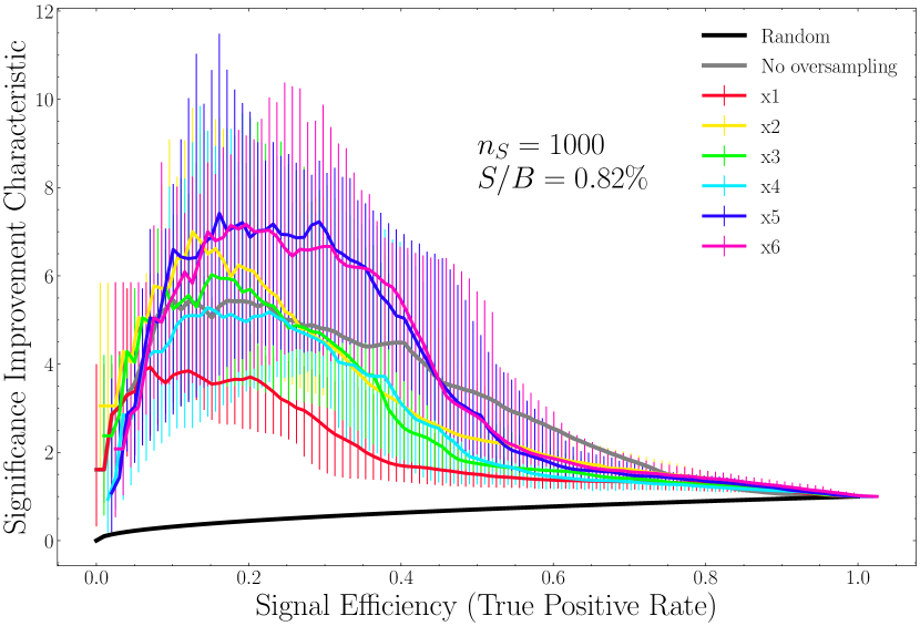
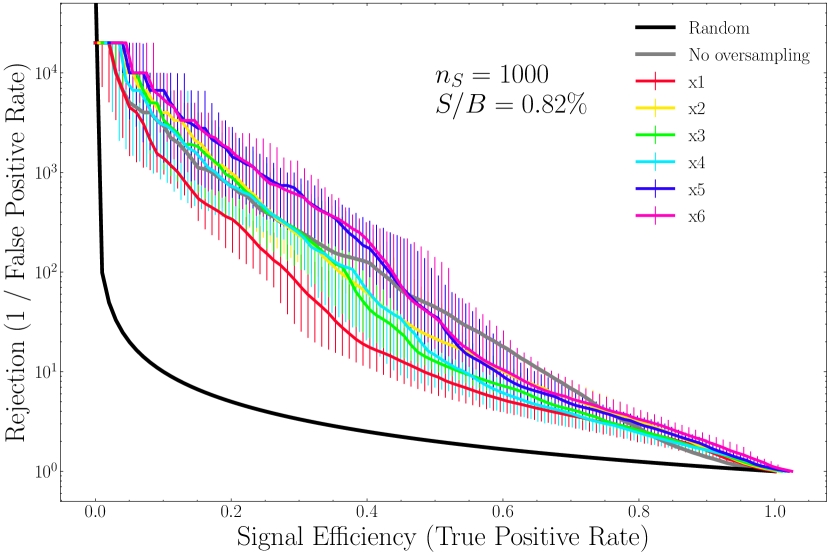
In Fig. 8(a) and Fig. 8(b), we plot the SIC and rejection (respectively) curves corresponding to oversampling factors from one (120k SR events) through six (720k SR events) for a signal injection of 1000 ($S/B=0.99\%)$. We find that the classifier performance generally increases to a peak at the oversampling factor of $\times$5, after which performance saturates. However, for signal injections of $\geq 2000$ ($S/B=1.97\%$), all oversampling factors perform similarly.

(a) Significance Improvement Characteristic

(b) Rejection

Figure 8: Performance metrics for a binary classifier trained to discriminate a constructed SM background template from detected SR data (with 1000 injected signal events) at various factors of oversampling. We retrain the binary classifier 20 times, each with a different random seed. Curves illustrate the median of these classifier runs, and bands represent the spread across the (16, 84) percentiles.

Appendix B Signal vs. Background Correlation

In this section, we compare in more detail the events produced by the various SM background template construction methods (Feta, Cathode, Curtains, and Salad).

We expect all of the methods to produce background samples that are significantly different from anomalous events. This is what allows us to detect resonant anomalies when training a classifier to discriminate between SR background samples and SR detected data. However, it is not obvious (or expected) that the background samples will be similar between methods. In fact, we might expect classifier scores to be uncorrelated for background events.

(a) Feta vs. Cathode.

(b) Feta vs. Curtains.

(c) Feta vs. Salad.

Figure 9: Classifier scores for a binary classifier trained to discriminate a given constructed SM background template from detected SR data with no injected signal events and evaluated on pure signal and pure background. The scores have been normalized to have zero mean and unit variance.

(a) Feta vs. Cathode.

(b) Feta vs. Curtains.

(c) Feta vs. Salad.

Figure 10: Classifier scores for a binary classifier trained to discriminate a given constructed SM background template from detected SR data with 2500 injected signal events and evaluated on pure signal and pure background. The scores have been normalized to have zero mean and unit variance.

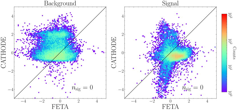
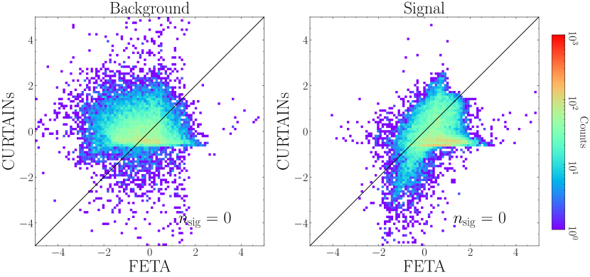
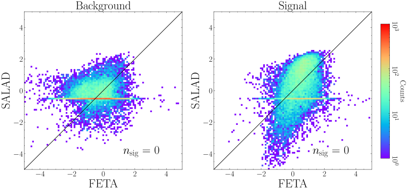
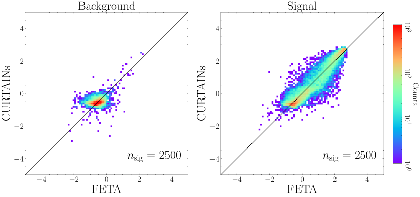
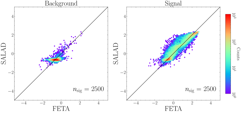
To probe how different the phase spaces are between construction methods: we train a binary classifier (with the architecture as described in Sec. III.2) to discriminate between SR background samples from SR detected data with 0 injected signal events. We evaluate the trained classifier on the test set of 20k signal and 20k background dijet events to get a score between 0 and 1 for each event. (Note that these scores are different than the AUC scores considered in the main analysis.) We finally plot these scores (standardized to zero mean and unit variance) for different methods as a function of each other, for Feta vs. Cathode in Fig. 9(a), for Feta vs. Curtains in Fig. 9(b), and for Feta vs. Salad in Fig. 9(c).

For both such cases, we find that the scores assigned to background events derived from classifiers trained on SM background samples from Feta are broadly uncorrelated with those from classifiers trained on SM background samples from the other three methods. There is perhaps a mild degree of correlation between scores for signal events, but the correlation would not be expected to be strong as the classifiers saw no signal events during training.

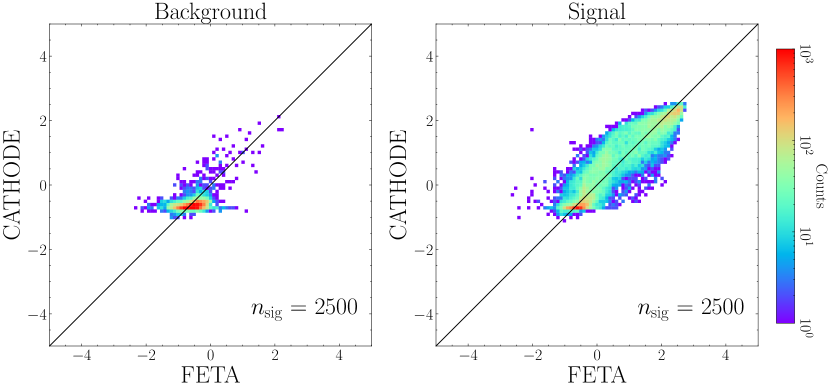
We then repeat the analysis, this time training the classifiers to discriminate between SR background samples from SR detected data with 2500 injected signal events. We plot the same standardized scores for Feta vs. Cathode in Fig. 10(a), for Feta vs. Curtains in Fig. 10(b), and for Feta vs. Salad in Fig. 10(c).

In these cases, there is a large degree of correlation between the classifier scores assigned to signal events between Feta and all of the other construction methods. This result indicates that all of the SM background construction methods are (roughly) equally sensitive to this particular LHCO anomaly.

References

- Karagiorgi et al. (2022) Georgia Karagiorgi, Gregor Kasieczka, Scott Kravitz, Benjamin Nachman, and David Shih, “Machine learning in the search for new fundamental physics,” Nature Rev. Phys. 4, 399–412 (2022).
- Kasieczka et al. (2021) Gregor Kasieczka et al., “The LHC Olympics 2020 a community challenge for anomaly detection in high energy physics,” Rept. Prog. Phys. 84, 124201 (2021), arXiv:2101.08320 [hep-ph] .
- Aarrestad et al. (2022) Thea Aarrestad et al., “The Dark Machines Anomaly Score Challenge: Benchmark Data and Model Independent Event Classification for the Large Hadron Collider,” SciPost Phys. 12, 043 (2022), arXiv:2105.14027 [hep-ph] .
- Benkendorfer et al. (2021) Kees Benkendorfer, Luc Le Pottier, and Benjamin Nachman, “Simulation-assisted decorrelation for resonant anomaly detection,” Phys. Rev. D 104, 035003 (2021), arXiv:2009.02205 [hep-ph] .
- Amram and Suarez (2021) Oz Amram and Cristina Mantilla Suarez, “Tag n’ train: a technique to train improved classifiers on unlabeled data,” Journal of High Energy Physics 2021 (2021), 10.1007/jhep01(2021)153.
- Choi et al. (2020) Suyong Choi, Jaehoon Lim, and Hayoung Oh, “Data-driven Estimation of Background Distribution through Neural Autoregressive Flows,” (2020), arXiv:2008.03636 [hep-ph] .
- CMS (2022) “Evidence for the simultaneous production of four top quarks in proton-proton collisions at = 13 TeV,” (2022).
- Andreassen et al. (2020) Anders Andreassen, Benjamin Nachman, and David Shih, “Simulation Assisted Likelihood-free Anomaly Detection,” Phys. Rev. D 101, 095004 (2020), arXiv:2001.05001 [hep-ph] .
- Stein et al. (2020) George Stein, Uros Seljak, and Biwei Dai, “Unsupervised in-distribution anomaly detection of new physics through conditional density estimation,” in 34th Conference on Neural Information Processing Systems (2020) arXiv:2012.11638 [cs.LG] .
- Nachman and Shih (2020) Benjamin Nachman and David Shih, “Anomaly Detection with Density Estimation,” Phys. Rev. D 101, 075042 (2020), arXiv:2001.04990 [hep-ph] .
- Hallin et al. (2022a) Anna Hallin, Joshua Isaacson, Gregor Kasieczka, Claudius Krause, Benjamin Nachman, Tobias Quadfasel, Matthias Schlaffer, David Shih, and Manuel Sommerhalder, “Classifying anomalies through outer density estimation,” Phys. Rev. D 106, 055006 (2022a), arXiv:2109.00546 [hep-ph] .
- Hallin et al. (2022b) Anna Hallin, Gregor Kasieczka, Tobias Quadfasel, David Shih, and Manuel Sommerhalder, “Resonant anomaly detection without background sculpting,” (2022b), arXiv:2210.14924 [hep-ph] .
- Raine et al. (2022) John Andrew Raine, Samuel Klein, Debajyoti Sengupta, and Tobias Golling, “CURTAINs for your Sliding Window: Constructing Unobserved Regions by Transforming Adjacent Intervals,” (2022), arXiv:2203.09470 [hep-ph] .
- Kobyzev et al. (2021) Ivan Kobyzev, Simon J.D. Prince, and Marcus A. Brubaker, “Normalizing flows: An introduction and review of current methods,” IEEE Transactions on Pattern Analysis and Machine Intelligence 43, 3964–3979 (2021).
- Tabak and Turner (2013) E. G. Tabak and Cristina V. Turner, “A family of nonparametric density estimation algorithms,” Communications on Pure and Applied Mathematics 66, 145–164 (2013), https://onlinelibrary.wiley.com/doi/pdf/10.1002/cpa.21423 .
- Durkan et al. (2020) Conor Durkan, Artur Bekasov, Iain Murray, and George Papamakarios, “nflows: normalizing flows in PyTorch,” (2020).
- Paszke et al. (2019) Adam Paszke, Sam Gross, Francisco Massa, Adam Lerer, James Bradbury, Gregory Chanan, Trevor Killeen, Zeming Lin, Natalia Gimelshein, Luca Antiga, Alban Desmaison, Andreas Kopf, Edward Yang, Zachary DeVito, Martin Raison, Alykhan Tejani, Sasank Chilamkurthy, Benoit Steiner, Lu Fang, Junjie Bai, and Soumith Chintala, “Pytorch: An imperative style, high-performance deep learning library,” in Advances in Neural Information Processing Systems 32 (Curran Associates, Inc., 2019) pp. 8024–8035.
- Klein et al. (2022) Samuel Klein, John Andrew Raine, and Tobias Golling, “Flows for flows: Training normalizing flows between arbitrary distributions with maximum likelihood estimation,” (2022).
- Kingma and Ba (2014) Diederik P. Kingma and Jimmy Ba, “Adam: A method for stochastic optimization,” (2014).
- Loshchilov and Hutter (2016) Ilya Loshchilov and Frank Hutter, “SGDR: stochastic gradient descent with restarts,” CoRR abs/1608.03983 (2016), 1608.03983 .
- Huang et al. (2018) Chin-Wei Huang, David Krueger, Alexandre Lacoste, and Aaron Courville, “Neural autoregressive flows,” (2018).
- Germain et al. (2015) Mathieu Germain, Karol Gregor, Iain Murray, and Hugo Larochelle, “Made: Masked autoencoder for distribution estimation,” (2015), 10.48550/ARXIV.1502.03509.
- Kasieczka et al. (2019) Gregor Kasieczka, Benjamin Nachman, and David Shih, “Official Datasets for LHC Olympics 2020 Anomaly Detection Challenge (Version v6) [Data set].” (2019), https://doi.org/10.5281/zenodo.4536624.
- Bähr et al. (2008) Manuel Bähr, Stefan Gieseke, Martyn A. Gigg, David Grellscheid, Keith Hamilton, Oluseyi Latunde-Dada, Simon Plätzer, Peter Richardson, Michael H. Seymour, Alexander Sherstnev, and Bryan R. Webber, “Herwig++ physics and manual,” The European Physical Journal C 58, 639–707 (2008).
- Sjostrand et al. (2006) Torbjorn Sjostrand, Stephen Mrenna, and Peter Z. Skands, “PYTHIA 6.4 Physics and Manual,” JHEP 05, 026 (2006), arXiv:hep-ph/0603175 .
- Sjöstrand et al. (2015) Torbjörn Sjöstrand, Stefan Ask, Jesper R. Christiansen, Richard Corke, Nishita Desai, Philip Ilten, Stephen Mrenna, Stefan Prestel, Christine O. Rasmussen, and Peter Z. Skands, “An introduction to PYTHIA 8.2,” Comput. Phys. Commun. 191, 159–177 (2015), arXiv:1410.3012 [hep-ph] .
- de Favereau et al. (2014) J. de Favereau, C. Delaere, P. Demin, A. Giammanco, V. Lemaître, A. Mertens, and M. Selvaggi (DELPHES 3), “DELPHES 3, A modular framework for fast simulation of a generic collider experiment,” JHEP 02, 057 (2014), arXiv:1307.6346 [hep-ex] .
- Metodiev et al. (2017) Eric M. Metodiev, Benjamin Nachman, and Jesse Thaler, “Classification without labels: Learning from mixed samples in high energy physics,” JHEP 10, 174 (2017), arXiv:1708.02949 [hep-ph] .
- Collins et al. (2019) Jack H. Collins, Kiel Howe, and Benjamin Nachman, “Extending the search for new resonances with machine learning,” Phys. Rev. D99, 014038 (2019), arXiv:1902.02634 [hep-ph] .
- Collins et al. (2018) Jack H. Collins, Kiel Howe, and Benjamin Nachman, “Anomaly Detection for Resonant New Physics with Machine Learning,” Phys. Rev. Lett. 121, 241803 (2018), arXiv:1805.02664 [hep-ph] .
- Mastandrea and Nachman (2022) Radha Mastandrea and Benjamin Nachman, “Efficiently Moving Instead of Reweighting Collider Events with Machine Learning,” in 36th Conference on Neural Information Processing Systems (2022) arXiv:2212.06155 [hep-ph] .