Continual Learning Approaches for Anomaly Detection

Abstract

Anomaly Detection is a relevant problem that arises in numerous real-world applications, especially when dealing with images. However, there has been little research for this task in the Continual Learning setting. In this work, we introduce a novel approach called SCALE (SCALing is Enough) to perform Compressed Replay in a framework for Anomaly Detection in Continual Learning setting. The proposed technique scales and compresses the original images using a Super Resolution model which, to the best of our knowledge, is studied for the first time in the Continual Learning setting. SCALE can achieve a high level of compression while maintaining a high level of image reconstruction quality. In conjunction with other Anomaly Detection approaches, it can achieve optimal results. To validate the proposed approach, we use a real-world dataset of images with pixel-based anomalies, with the scope to provide a reliable benchmark for Anomaly Detection in the context of Continual Learning, serving as a foundation for further advancements in the field.

Keywords Anomaly Detection  $\cdot$ Continual Learning  $\cdot$ Catastrophic Forgetting  $\cdot$ Incremental Learning

1 Introduction

Anomaly Detection (AD) is an important and challenging problem in the field of Machine Learning (ML) and Computer Vision. Anomalies are patterns characterized by a noticeable deviation from the so-called normal data, where normal means compliance with some typical or expected features [1]. In order to effectively detect anomalies, it is important to have a clear understanding of what constitutes normal behavior and how to differentiate it from abnormal patterns.

Current state-of-the-art neural networks have achieved exceptional performance in solving a wide range of classification and detection tasks, especially in Computer Vision. However, these algorithms struggle to learn multiple tasks in succession. As a result, they are prone to Catastrophic Forgetting (CF): when learning a new task, artificial neural networks frequently forget the previous ones [2]; this significantly hinders the adoption of these approaches in real-world scenarios. To address this issue, a new branch of machine learning has been introduced, known as Continual Learning (CL) [3]. CL focuses on learning new tasks without forgetting the previous ones.
In this work, we define a general framework for Anomaly Detection in the Continual Learning (ADCL) setting, within which we investigate various architectures and CL strategies.

Several CL strategies have been developed in the literature in recent years to prevent catastrophic forgetting. Replay is the most well-known and effective method for preventing forgetting [4, 5]. It consists in storing some samples in raw format and passing them during the subsequent tasks. One of the main issues with such an approach is that memory size is limited. To address this issue, some Compressed Replay (CR) methods have recently been developed with the idea of compressing the samples to increase the number of stored images with the same memory size. In the same vein, we consider Compressed Replay for Anomaly Detection in the Continual Learning setting. The proposed framework consists of two modules, that may coincide in some cases: (i) a Memory module that enables Compressed Replay; (ii) an Anomaly Detection module that is able to learn how to distinguish anomalies for new classes without forgetting how to deal with previously learned ones.
Within the proposed framework for ADCL, we evaluate different approaches. In particular, as for the Memory Module we propose using a cGAN [6] with the Super Resolution (SR) objective to obtain compressed representations.

Concerning the AD module, we study both generative and features-based [7] approaches. While generative models can achieve both CR and AD, feature-based models can only perform AD but do not enable CR. In this work, we propose using SCALE for CR, in conjunction with feature-based AD models, demonstrating that such a combination can achieve optimal performance. To investigate the performance of different choices for the Memory and the AD module in the ADCL framework, we propose to use MVTec dataset as a benchmark [8]. It is designed to be representative of many challenges of real-world pixel-level AD. Furthermore, this dataset provides 10 classes of objects that can be used as consecutive tasks to be learned in a CL setup.
To recap, the main contribution of this work is three-fold:

1. We design a general framework to solve an AD problem in a CL setting.

2. We propose a novel approach for ADCL where SR models are used to achieve Compressed Replay for the first time, to the best of our knowledge.

3. We propose to use the MVTec AD dataset as a new Continual Learning benchmark for Anomaly Detection [8].

The outline of the paper is the following. In Section 2, we describe related work in terms of AD, AD for CL, and Compressed Replay. In Section 3, we introduce the framework proposed for AD and describe the CL strategies and architectures considered. In Section 3.3, we describe our novel approach for Compressed Replay based on an SR model to retain the knowledge of old tasks. In Section 5, we describe the experimental setup that implements our approach, including details about the evaluation metrics used, the dataset, and the CL setting proposed. Finally, in Section 6, we present our findings before concluding in Section 7.

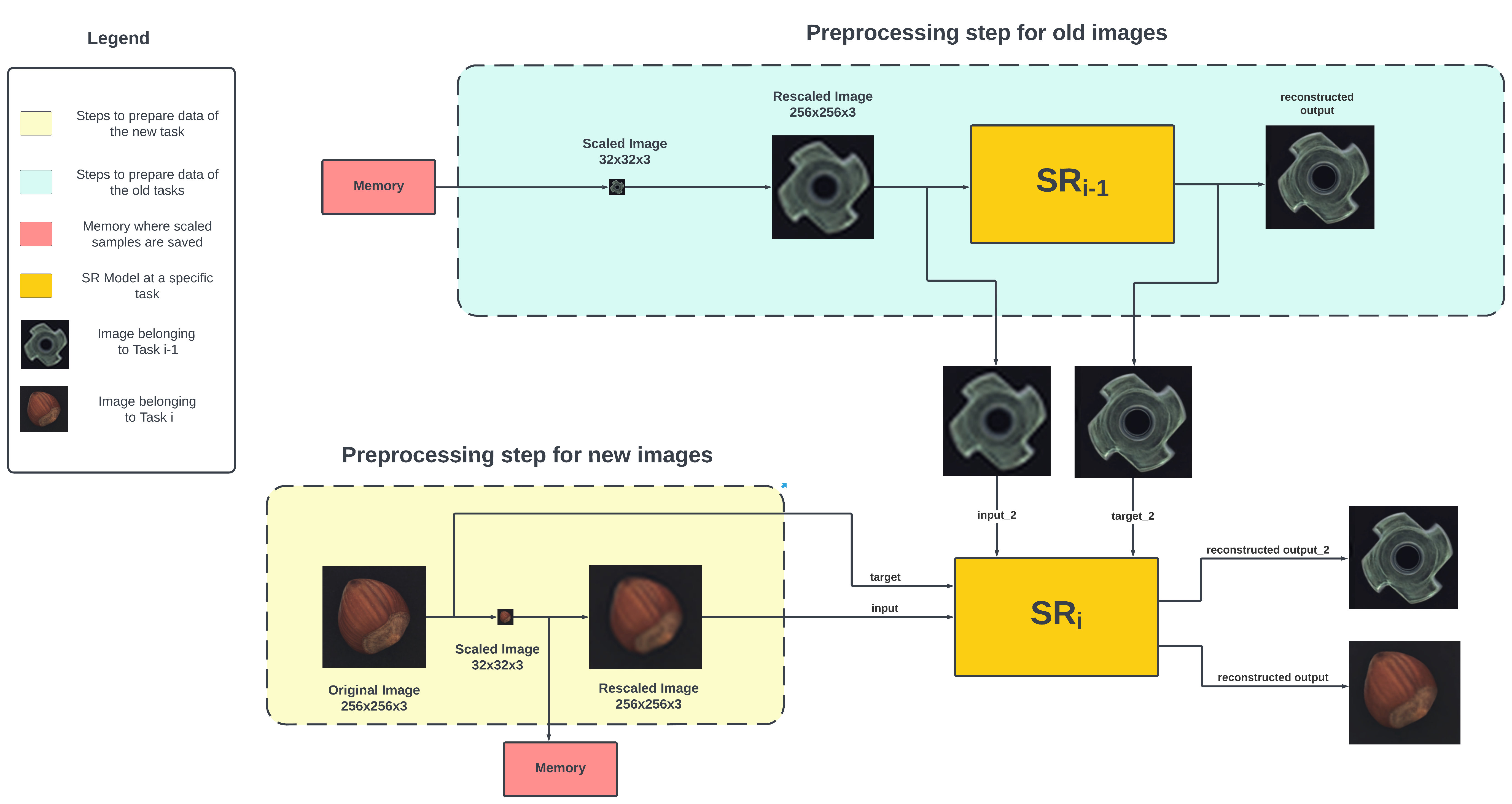
Figure 1: Scheme of the proposed approach for compressed Replay called SCALE. To perform Super Resolution (SR), we use a Pix2Pix architecture. First, the current task images are scaled (compressed) and saved in memory (yellow area). Then, they are rescaled ($input$), and the model is trained to reconstruct the original image ($target$). Instead, for old tasks, the images are taken from memory, rescaled, and reconstructed using the SR model from the previous task, in order to retain old knowledge (light blue area). After that, the rescaled blurry image ($input_{2}$) is fed into the current SR model, with the target corresponding to the image reconstructed by SR in Task $i-1$ (i.e., $target_{2}$).

2 Related Work

In this section, we first summarize the challenges of Continual Learning with a focus on approaches based on Replay. Then, we review some contributions devoted to Anomaly Detection in the Continual Learning scenario. Finally, we mention some non-continual Anomaly Detection approaches evaluated on the MVTec dataset.

2.1 Compressed Replay for Continual Learning

Continual learning provides ML models with the ability to update and expand their knowledge over time, with minimal computation and memory overhead [3]. Thus, an effective CL solution is expected to have low forgetting, require low memory consumption and be computationally efficient. CL strategies are usually classified into three categories: replay-based [9, 10, 11] methods, regularization-based [12, 13, 14] methods and architectural-based [15, 16] methods. The related literature suggests that the Replay (also known as Rehearsal) approach appears to be the most effective and practical solution to reduce CF [17, 18, 19, 20].

The simplest implementation, known as Experience Replay (ER) [10, 21] consists in storing some samples in the raw format selected randomly from the current task and passing them during the subsequent tasks. Therefore, during training, each batch of data from the current task is combined with a batch of data from the previous tasks (sampled among them with the same probability). However, the memory storage limit is a significant constraint, the smaller the memory size, the further we are from the original training distribution of old tasks.

Methods for reducing the storage cost of old training samples have recently been developed for this problem. We refer to them as Compressed Replay, where the goal is to learn a compressed data representation. The most important and vast family of this field is Latent Replay. Latent Replay methods propose to store activations from an intermediate layer of a neural network and Replay these representations to prevent forgetting. Typically, in a classification task, these encodings are used as Replay starting from a specific layer, as done in [18], where lower layers are trained at a slower pace to avoid latent representation shift. In [22] authors propose to use pre-trained models to extract features and use them for training a classification model. They study the performance of Replay and Latent Replay using several pre-trained models. In [23], the lower layers are frozen, and only the upper layers are trained. Moreover, to store more samples, they propose to use Product Quantization (PQ) to compress and save the features efficiently, obtaining a compression factor of around 50. In [24] authors propose to apply feature adaptation so that features learned for the old task remain consistent with the new feature space.

The previous works were done for the classification problem, and the compression factor depends on the size of the layer chosen to extract the features to store in memory, so different compression factors can be obtained depending on the chosen layer. However, because we are interested in generative problems, we want to be able to compress the original samples while retaining the ability to reconstruct the original image in the output. For instance, in [25] authors propose EEC, a Generative Replay approach that also memorizes the centroid and covariance of each class to make the training more stable. In [26] authors introduce the use of Adaptive Quantization Modules(AQM) to Continual Compression on the LiDAR dataset and also allow the selection of the trade-off between the compression factor and quality of reconstructed images.

Many generative models, as described in Section 5, can be used for Latent Replay. However, no research on generative models regarding Latent Replay was conducted. Therefore, as an additional contribution, we also provide an accurate comparison of several generative models for Latent Replay, examining their efficacy in terms of compression factor and image quality. Moreover, we propose a novel approach for Compressed Replay called SCALE and described in Section 3.3. This approach shows a high level of compression and at the same time, a high level of quality in the generated images.

2.2 Anomaly Detection in the Continual Learning setting

Despite the fact that it is extremely relevant in practice, only a few works in the literature addressed the AD problem in the CL setting.

In [1], the authors propose using the Variational Autoencoder (VAE) with the Generative Replay approach to learn continually new classes while also performing AD. The datasets used in the evaluation are KDD Cup 1999 and MNIST, which have been artificially adapted to AD by marking one of the classes as anomalous. In [27], using the same dataset KDD Cup ’99 and other datasets belonging to Network Intrusion Detection, the authors study the problem of AD formulated as a binary classification supervised learning. The authors of [28] propose a regularization-based approach for continual AD in manufacturing, and evaluate it on a real industrial metal forming dataset.

As for AD for images, the majority of work in this field focuses on predicting whether an image is normal or abnormal. However, in practice, anomaly localization is frequently required. Not only is it necessary to explain the predictions, but it is also necessary to perform root cause analysis. As a result, we investigate a complex image dataset such as MVTec, which contains pixel-based anomalies. We also investigate a wide range of models and assess their performance.

2.3 Approaches for MVTec AD Dataset

In the literature, many non-continual approaches for pixel-level Anomaly Detection are tested on the MVTEc dataset. We can split most of them into reconstruction-based and embedding similarity-based methods.

Reconstruction-based methods learn to reconstruct normal images during training. However, during the evaluation, images with defects are not expected to be reconstructed well. Consequently, they should exhibit a higher reconstruction error than normal images. Reconstruction-based methods include neural network architectures like autoencoders [8, 29, 30], variational autoencoders [31] and generative adversarial networks [32, 33]. The idea is that autoencoders will ignore minor details that don’t belong to the training distribution and reconstruct the image without the defects. However, they can sometimes reconstruct defects in output, leading to a failure to distinguish between abnormal and normal images.
In [34] an approach based on inpainting is proposed called RIAD. The idea is to hide a portion of the input image and train the model to reconstruct it.
In the same spirit, we consider Super Resolution to solve Anomaly Detection. In this method, the image is scaled to a lower resolution and then rescaled to the original size, resulting in a loss of information about the original image. The concept is similar to inpainting because a portion of the information in the images is hidden. Then the model is trained to reconstruct the image while also repairing the defects in the original image.

Embedding similarity-based methods, on the other hand, use pre-trained neural networks to extract meaningful features from images. These kinds of techniques proved to be the state of the art of the field. SPADE [35] first performs image feature extraction based on a WideResNet50 [36] trained on ImageNet [37], then retrieves the K-nearest normal images, and finally achieves pixel alignment with deep feature pyramid correspondences. Similarly to SPADE, PaDiM [38] relies on ImageNet pre-trained feature extractor with multi-scale pyramid pooling. However, instead of k-nearest neighbor clustering, it computes an anomaly score based on the Mahalanobis distance. Normalizing Flows  (NF) [39, 40]  are a powerful tool for modeling complex distributions, such as those that arise in Anomaly Detection tasks.  By embedding normal data into a high-dimensional standard normal distribution, it becomes possible to use the probability of the data under the distribution as a measure of its normality.  This can be useful for identifying and localizing anomalies in data. For example, in the case of image data, normalizing flows can be used to model the distribution of image features, and then use the probability of a given image under the distribution to identify and locate anomalies in the image. FastFlow and CFLOW-AD are two examples of methods that use normalizing flows for anomaly detection, with FastFlow focusing on improving anomaly localization by using a 2D flow model.

3 Proposed Framework for Anomaly Detection in Continual Learning setting

3.1 Problem Definition

Anomaly detection is a challenging task, particularly when the data contains distinct objects. In this case, abnormal samples are often much closer to normal ones than to samples from other classes. This is illustrated in Figure 2, where different colors represent different object classes, normal samples are depicted as circles, and anomalies are depicted as crosses. The closeness of the anomalies to the normal samples makes it difficult to identify and distinguish them using traditional methods. The task becomes even more challenging when we want to identify if the single pixel of an image is an anomaly or not in the CL setup where new objects must be learned subsequently.

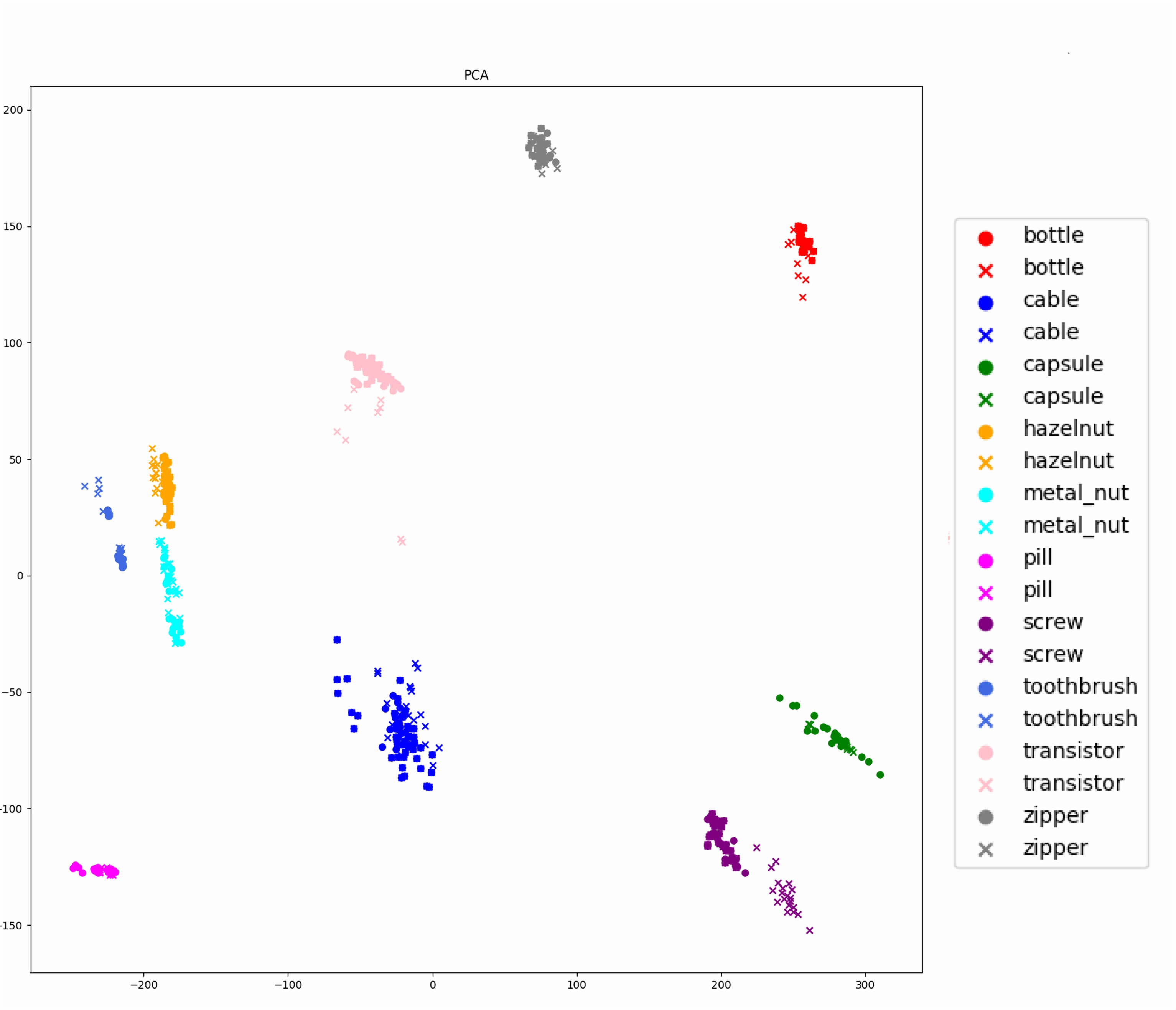
Figure 2: We show the PCA on the original images where the first two dimensions capture 73% of the total variance. Each class is depicted in a different colour, with circles representing normal images and crosses representing abnormal images. As can be seen, the separation between normal and abnormal samples coming from the same class is much lower than the distance between classes. The actual scenario is even more challenging since we aim at detecting pixel-level instead of image-level anomalies.

The goal is to train a neural network model that can detect anomalies while also retaining the knowledge it has learned from previous tasks. The model is trained on a sequence of tasks, each of which corresponds to one or more object classes. During training, the model learns the distribution of normal (i.e., anomaly-free) images for each task. Then, during evaluation, the model is tested on a dataset that contains data from all tasks, both normal and abnormal. This allows the model to detect anomalies in the test data by comparing it to the learned distribution of normal data.

In more formal terms, ADCL is a method for learning a model that can detect anomalies in data. The model is trained on a sequence of tasks with a total of $T$ tasks. Each Anomaly Detection task $t$ corresponds to a dataset $D_{t}$.  Each dataset $D_{t}$ consists of pairs of data $(X_{t},Y_{t})$, where $X_{t}$ is a set of images  or more formally $X_{t}\subset\mathbb{N}^{H\times W\times 3}$ where $H$ and $W$ denote the spatial dimensions and $t=1\cdots T$.  $Y_{t}$ is a set of labels for each pixel of the image, indicating whether the pixel is normal (0) or anomalous (1). The goal of the model is to learn a mapping $f_{\theta}:X\rightarrow R^{H\times W}$ from the space of images $X$ to a probability vector. This allows the model to assign a probability to each pixel in an image, indicating how likely it is to be normal or anomalous.

In the field of continual learning (CL), there are three main scenarios that are commonly studied: Task Incremental Learning (TIL), Domain Incremental Learning (DIL), and Class Incremental Learning (CIL) [2, 41]. In our problem, we are dealing with the DIL scenario because the classes of output remain fixed independently by the change of task (i.e. there are always only two classes, normal and abnormal, for each pixel of the image), while the input distribution changes between tasks i.e. $P(X)\neq P(X^{\prime})$.

3.2 Proposed ADCL Framework

We introduce a general framework for ADCL. We present a general framework for the task of Anomaly Detection in Continual Learning (ADCL). The goal of this framework is to enable incremental learning of new objects while also detecting anomalies in images from previous tasks. The proposed framework, depicted in Fig. 3, is broken down into two modules:

1. Memory Module: This component’s goal is to retain the memory of previous tasks. Depending on the type of CL strategy considered, such a module may take various forms. In the case of Replay, for example, such a module consists of a limited memory containing some of the images of previous tasks. In the case of Latent Replay, the module will consist of an autoencoder (AE) and a set of compressed samples memorized through the latent space. In the case of regularization-based strategies, such as EWC [42], the Memory Module will be composed of the importance values associated with each weight of the architecture used in the AD Module.

2. AD Module: It is the architecture used to detect anomalous pixels. The chosen architecture can be any previously proposed approaches, like AE, VAE, and GANs for reconstruction-based approaches or FastFlow, and CFlow for embedding similarity-based.

It is important to note that the Memory Module and the AD Module are typically described as separate functional entities, but the same model can serve both functions. For example, many reconstruction-based methods can generate images of old tasks for use during the training of a new task, the ability to reconstruct images can also be used for anomaly detection by comparing the reconstructed image to the original image.

The Memory Module is a key component of a Continual Learning (CL) system, responsible for storing and updating information about previous tasks. This module is updated using a combination of data from the current task and a batch of old data from the previous task, as depicted in Fig. 3. In the case of classic Replay, the Memory Module simply stores images. With Latent Replay and generative models such as CAE or VAE, the Memory Module stores the model of the previous task and samples in the latent space, which allows for more efficient storage of images compared to Replay. It is also possible to use Generative Replay with VAE and GAN models, but it has been shown to result in a high degeneration [43].

3.3 SCALE: A novel approach for Compressed Replay

Within the above-introduced framework for Visual Anomaly Detection in Continual Learning, we proposed SCALE (SCALing is Enough), a Super Resolution-based approach, as a Compressed Replay technique. Super Resolution aims to convert a low-resolution image with coarse details into a high-resolution image with improved visual quality and refined details [44]. In practice, as SR model, we consider the Pix2Pix [6], a general-purpose model for image-to-image translation composed of a conditional GAN [45]. The cGAN, unlike the classic GAN [45], is conditioned not only by random noise but also by an input image. The GANs have the flaw of having a high forgetting with Generative Replay (where the images are generated using random noise) [43]. We show how conditioning to an input image plus the noise can result in a method that can still generate images with a low forgetting even though the output still has a random component. Though such architecture is not the state-of-the-art of the SR field, it is sufficient to obtain good results and justify its use in this context, as shown in Section 6. Therefore, in our work, the SR model is studied with three final objectives:

1. Since it is the first time that the SR problem is studied in CL, we provide an evaluation in terms of reconstruction of the original images and how this approach behaves in terms of forgetting.

2. We also investigate the use of memory in combination with AD approaches that are by nature not able to perform the function of memory.

3. We consider the efficacy of SR in terms of AD.

The proposed schema for using the SR model in Continual Learning is shown in Fig. 1 and can be summarized in the following steps:

1. When a new task is received, the images are resized to a lower resolution and a copy is saved in memory. The objects saved for a task will remain unchanged during training, as opposed to Replay and Latent Replay.

2. The process for handling the images of the new task is depicted in the yellow portion of Fig. 1. The other image is resized again (which reduces its quality) and sent to the SR model to learn how to reconstruct the original image.

3. The procedure to obtain images of old tasks to be used in the training of current tasks is depicted in Fig. 1 as the light blue part. To obtain images from old tasks to use in training the current tasks, the scaled image saved in memory of shape (32,32,3) is rescaled to its original size (256,256,3) and labeled as $input_{2}$ in Fig. 1. Then it is passed to the SR model to obtain an image quality similar to the original, such output is labeled as $target_{2}$ in Fig. 1. The SR model of the current task is then trained to reconstruct the rescaled image ($input_{2}$) using the reconstructed image ($target_{2}$).

By memorizing the scaled images and increasing the resolution when needed, it is possible to achieve a compression factor. The value of such compression depends on the final quality that is desired, and it will depend on the final scope.
We are going to present its results in terms of performance for Anomaly Detection in Section 6.1 and in terms of the quality of reconstructed images in the Section 6.2. Because this is the first time that SR has been studied in the context of CL, we present additional results for such a model in Section 6.3 where we explain why it works compared to classic GANs and its advantages. Among the results, it is shown to be advantageous to keep the memory of a task fixed over time rather than changing continuously as is typical in Latent Replay.

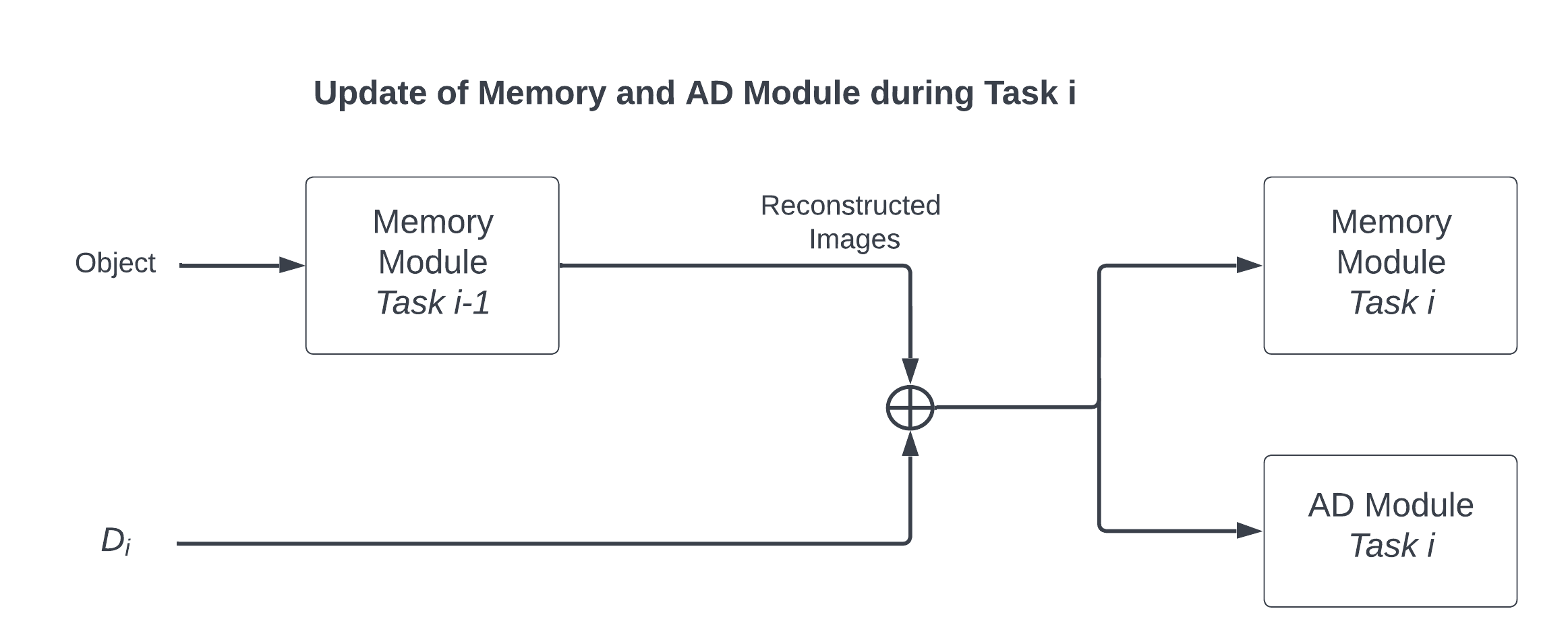
Figure 3: The proposed framework is composed of 2 modules: memory and Anomaly Detection. The Memory Module will be updated using the data from the current task as well as a batch of old data retrieved using the Memory Module of previous task.

4 Considered Benchmark Dataset

We propose to use the MVTec Dataset [8] as a benchmark to study the performance of architectures and CL strategies for Anomaly Detection. The MVTec AD dataset is a recent and extensive industrial dataset that includes 5354 high-resolution images divided into 15 categories: 5 types of textures and 10 types of objects. The training set only contains normal images, whereas the test set includes both defect and defect-free images. The image resolutions range from (700,700,3) to (1024,1024,3) as resolution. In our ADCL framework, we will consider a sequence of 10 tasks. Each task corresponds to one of the 10 classes associated with objects. In this study, the model is presented with a series of tasks, and must be able to identify which pixels in the image are abnormal for each object. The MVTec dataset used in this study is more challenging and complex than the commonly used datasets MNIST and CIFAR-10, which are often used in Continual Learning literature [46, 47, 48]. These datasets have smaller image sizes, (28,28) for MNIST and (32,32) for CIFAR-10, and fewer images, making them not as representative of real-world scenarios as the MVTec dataset.

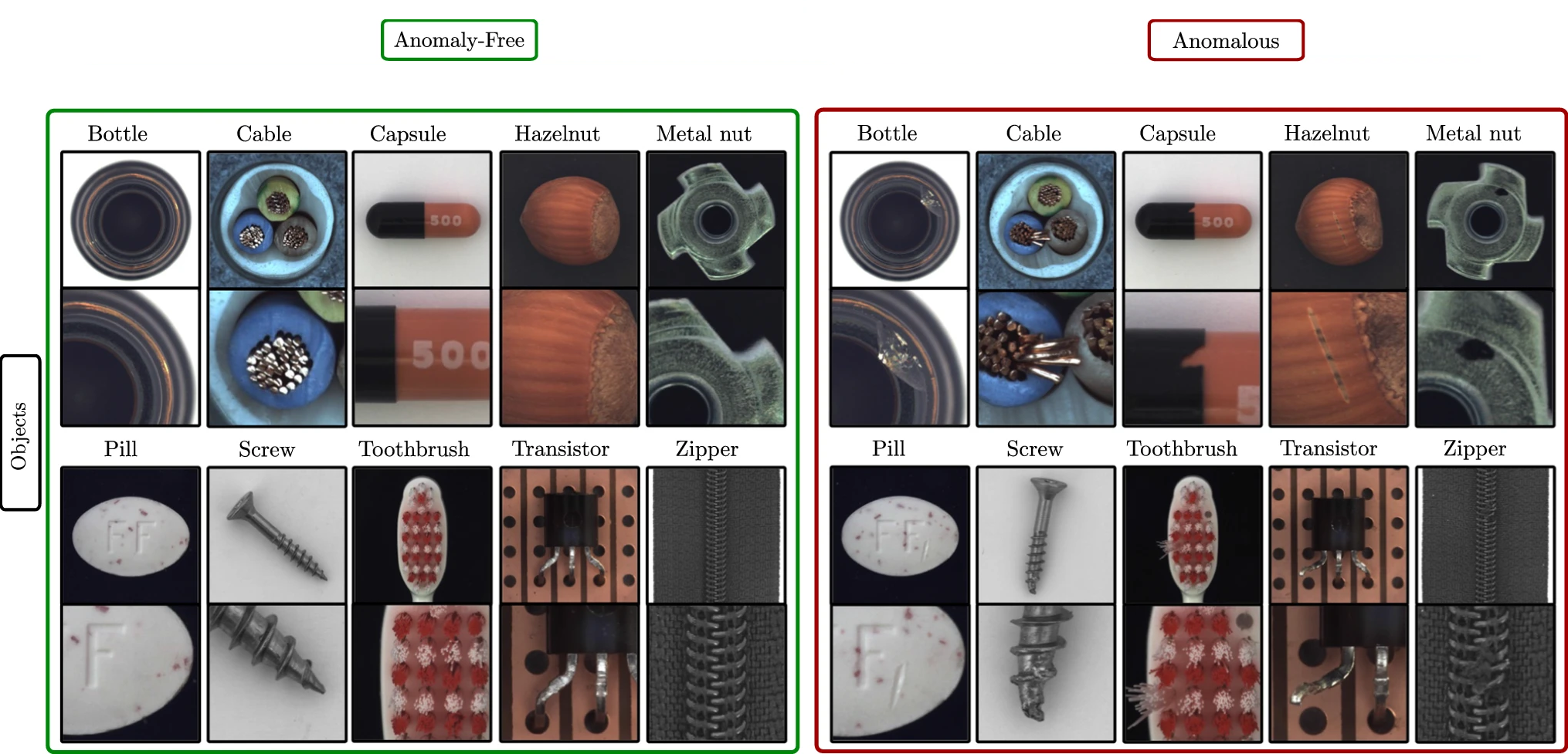
Figure 4: Image examples from the MVTec Dataset AD. For each object is shown a normal sample (in green) and an anomalous sample (in red). For each sample, the entire object is displayed, as well as a zoomed-in view of the region containing the defect. The samples illustrate the range of variations and abnormalities that can be found in the dataset.

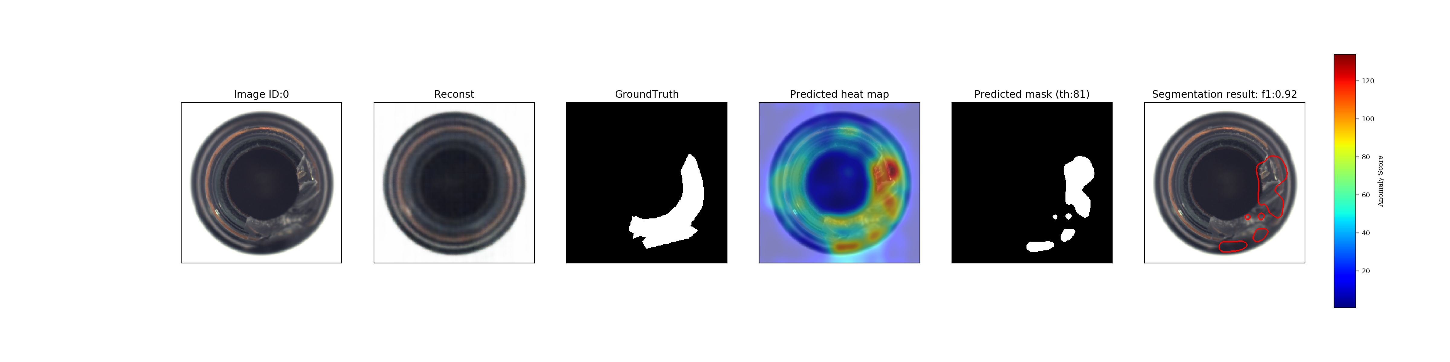
(a) Reconstruction based on VAE

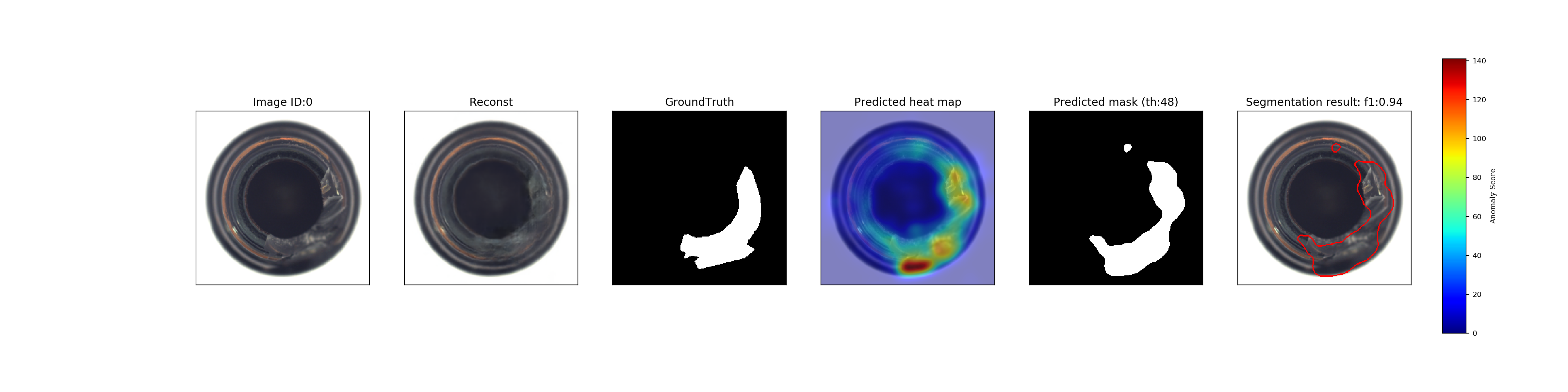
(b) Reconstruction based on SR

Figure 5: The images reported here show examples of the VAE (Variational Autoencoder) architecture in (a) and the SR (Super-Resolution) architecture in (b). The first image in each row is the original image, and the second column is the model’s reconstructed image. The third column displays the ground truth for each pixel, which can be used to evaluate the accuracy of the reconstructed image. The fourth column shows the anomaly map, which indicates the probability that each pixel is abnormal (i.e., significantly different from the original pixel). This can help identify corrupted areas of the image. The fifth column displays the predicted class for each pixel, which provides more information about the model’s final prediction on what is considered anomalous. The sixth column highlights any potential issues with the image by showing the anomalous parts of the image, making it easier for users to identify and address any problems.

5 Experimental Settings

5.1 Considered CL Strategies

We are going to evaluate the different architectures in terms of performance for both the Memory Module and the AD Module. Such evaluation will be performed considering different CL strategies that will be applied to the models.

• Single Model: As an upper bound, we train a different model for each task.

• Fine-tuning: As a lower bound, we consider the fine-tuning approach, in which a model is presented sequentially only with data from the current task.

• Ideal Replay: As a benchmark Continual Learning strategy, we consider an approach where we randomly select $n$ images from a task and create a training batch with half data from the current task and half data from previous tasks. The constraint on processing power is respected, but not the constraint on memory. Indeed, this approach takes into memory all samples seen so far. This implies that the memory can capture the original distribution completely. We refer to this approach as Ideal Replay, and we propose to consider it as an additional upper bound for CL approaches.

• Replay: We consider a constrained memory size of $n$ images such that: $n<<|D|$ where $D$ represents the entire dataset. In the experiments, $n$ is set to $40$ images, representing less than $2\%$ of the total dataset. This means that the total memory size is limited to $40$ images, i.e., four images for each class at the end of the training.
  

• Compressed Replay: When dealing with Replay, we should keep in mind that the risk of overfitting is high when only a few samples represent a task. Given that memory size can influence final results, the ability to save more samples has the potential to reduce forgetting because the distribution in memory of an old task is more similar to the original one (assuming that the quality of compressed samples is high enough). So in Compressed Replay, the images are compressed. For example, in Latent Replay, we consider their representation in the latent space. Similar to Replay, we consider the constraints on processing power and memory size, but with Compressive Replay, we try to keep more images in memory by utilizing some compression method.
  When considering Latent Replay, because we will be studying architecture such as autoencoders, it is more natural to choose the latent space that corresponds to the Encoder’s output and the Decoder’s input, i.e. the bottleneck layer, which has the lowest dimensional space.

• Generative Replay: In the case of Generative Replay [9], we use models such as GANs to generate images without the need to store any additional information other than the model itself. This can be very useful because it eliminates the need to save any data in memory. However, in previous experiments [43], the Generative Replay had a high level of forgetting and much of the information was quickly lost.

To ensure a fair comparison between Compressed Replay and Replay, we use the same amount of memory in terms of bytes for both approaches. We define the memory size as $C$, which is the number of bytes needed to store $n$ images using the Replay strategy. For Compressed Replay, a number of compressed samples will be stored, taking up a maximum of $C$ bytes of storage.

In general, we will compare the different methods, with upper bounds included, taking into account that, on the practical side, the only valid CL approaches are Replay, Compressed Replay, and Generative Replay, since they are the only ones with a memory size and processing power constraint.

We will be comparing the Continual Learning strategies introduced above in terms of their performance in two key areas: Anomaly Detection and the quality of the reconstructed images. For the Compressed Replay strategy, we will also be considering the compression factor as a key metric. A higher compression factor means that more samples can be stored, but we must also take into account the quality of the reconstructed images. If the compression factor is high, but the quality of the reconstructed images is poor, then the distribution of the reconstructed images will be significantly different from the original distribution. It is important to find the right balance between these two factors to achieve optimal performance.

5.2 Considered Architectures in Memory and Anomaly Detection modules

The following models were considered as both Memory and AD modules:

• Convolutional Auto-Encoder(CAE): It has a latent space of shape (512,4,4) i.e. of dimension 8192, implying a compression factor value equal to 6 (assuming that we are working with 4 bytes for each value). Taking into account an input shape (256,256,3) we can simply calculate the compression factor as $\frac{196608}{8192\cdot 4}=6$. We will memorize the activations of the CAE obtained in the latent space in the case of Latent Replay.

• Variational Auto-Encoder(VAE): Using the VAE (Variational Autoencoder) architecture, we were able to achieve good results with a smaller latent space compared to the CAE (Convolutional Autoencoder). Specifically, we obtained a latent space dimension of 256 and a compression factor of 96. It is worth noting that the VAE architecture can be used not only with the Latent Replay strategy but also with Generative Replay, which allows the model to store information without any actual samples. However, as previously mentioned and shown by our results, the quality of the images generated by VAE with Generative Replay degrades quickly.

As for the approaches that can be used as AD Module only, we consider:

• Inpaint: We tried to use the same architecture of RIAD [30] in our study, but found that the architecture was very sensitive to the continual learning setting and we were unable to obtain satisfactory results. As an alternative, we adopted the spirit of the RIAD approach (i.e., inpainting) and proposed a different architecture, a Pix2Pix model [6], for the inpainting task. In our version, training is done by masking random areas of the images. During reconstruction, the same image is fed into the model multiple times (with different masks each time), and averaging is used if the same pixel is masked multiple times.

• FastFlow: We use FastFlow [49] in combination with the WideResNet50 [36]. This approach, described in Section 2, learns a Normalizing Flow that models normal images. It should be noted that this is one of the few studies on Normalizing Flow architectures in CL setting. To the best of our knowledge, only two other studies were done [50, 51].

5.3 Evaluation Metrics for Anomaly Detection

There are several metrics commonly used to evaluate the performance of Anomaly Detection models on the MVTec AD dataset. The ROC AUC score at the pixel and image levels is the most widely used, but other metrics such as f1 score and IoU are also taken into account. In the Anomaly Detection literature, it is generally believed that metrics such as the f1 score are more fair when dealing with imbalanced datasets, which is often the case with Anomaly Detection [52]. Therefore, in this study, we use the f1 score to assess a model’s ability to detect anomalies. A well-performing model should have a high f1 score and a low FID score.

5.4 Evaluation of image reconstruction quality

To evaluate the quality of the reconstruction performed by the models used in the Memory Module, we will use the Fréchet Inception Distance (FID) [53], which is a commonly used metric for evaluating generative models [43]. This type of evaluation is useful for analyzing the performance of all architectures that can function as Memory Modules under various CL strategies. The FID is calculated as:

$$FID=||\mu_{r}-\mu_{g}||^{2}+Tr(\Sigma_{r}+\Sigma_{g}-2(\Sigma_{r}\Sigma_{g})^{\frac{1}{2}})$$ (1)

The statistics $(\mu_{r},\Sigma_{r})$ and $(\mu_{g},\Sigma_{g})$ are the activations of a specific layer of a discriminative neural network trained on ImageNet for real and generated samples, respectively. A lower FID indicates that real and generated samples are more similar, as measured by the distance between their activation distributions.
Beyond the models that can be used in the Memory module, we will evaluate the image reconstruction quality also for Inpaint, even if it lacks the ability to compress them and to act as a Memory Module.

5.5 CL Metrics

Following the convention of Continual Learning we are going to considered the average value at the end of the training and the forgetting. Let $s_{i,j}$ be the performance f1 of the model on the test set of task $j$ after training the model on task $i$. To measure performance in the CL setting, we introduce the following metrics:

Average f1

The average f1 score $S_{T}\in[0,1]$ at task T is defined as:

$$S_{T}=\frac{1}{T}\sum_{j=1}^{T}s_{T,j}$$ (2)

Average Forgetting

$F_{T}\in[-1,1]$, the average forgetting measure at task T, is defined as:

$$F_{T}=\frac{1}{T-1}\sum_{j=1}^{T-1}max_{l\in\{1,\cdots,T-1\}}\frac{s_{l,j}-s_{T,j}}{s_{l,j}}.$$ (3)

With respect to the original definition used in [54], we are scaling respect to the maximum f1 score, as done in [20, 55]; this is done to compare the forgetting among tasks with very different scores. Notice that the closer the metric $F_{T}$ is to 1, the higher the forgetting is. What it was defined above for the metric f1 will be redefined in a very similar way for the metric FID, with the consideration that the goal of FID is to be minimized while with f1 we want to maximize it.

6 Experimental results

We will compare all models in terms of Anomaly Detection performance using the Average f1 score as a metric in Subsection 6.1. Then, in Section 6.2, we will try to motivate the results by evaluating the quality of reconstructed images produced by different models and CL strategies. Finally, because this is the first time (to the best of our knowledge) that a Super Resolution model has been studied in a Continual Learning setting, we investigate the results at a greater level in subsection 6.3. Each test is repeated ten times for each cell in the result tables, and only the average is shown. The plots shown in the Section Results will display the mean and variance of the runs. For the sake of reproducibility, the code used in the experiments is available in a public repository online.

6.1 Quality of the Anomaly Detection

Table 1: Summary table for the AD performance under different CL strategies and architectures for the Memory and the AD Module. Since Inpaint and FastFlow cannot achieve Compressed Replay, but only act as AD modules, we consider them in combination with CAE, VAE and SR as Memory Modules. We report the Average f1 value ($\uparrow$ stands for "the higher the better") and, within round brackets, the forgetting associated to the metric, for each combination. We highlight in bold the best combination. We can observe that, among the viable Replay-based strategies, the best combination is using Inpaint as AD Module with SR as Memory Module adopting the Compressed Replay strategy. The best combination is in bold while the best architecture for each strategy is in italic.

Strategy	Memory Module	AD Module (Average $\mathrm{f1}$ metric $\uparrow$ )
		CAE	VAE	SR	Inpaint	FastFlow
Single Model	-	0.28	0.36	0.33	0.38	0.57
FT	-	0.09 (66.35%)	0.11 (68.19%)	0.14 (59.39%)	0.11 (72.73%)	0.19 (69.79%)
Ideal Replay	-	0.28 (13.22%)	0.33 (6.38%)	0.36 (5.72%)	0.34 (11.25%)	0.22 (62.53%)
Replay	-	0.26 (19.88%)	0.30 (21.2%)	0.29 (22.23%)	0.34 (13.27%)	0.21 (64.57%)
Generative Replay	-	-	0.11 (63.68%)	-	-	-
Compressed Replay	CAE	0.23 (25.61%)	-	-	0.25 (34.00%)	0.17 (53%)
	VAE	-	0.25 (21.87%)	-	0.26 (30.27%)	0.2 (48%)
	SR	-	-	0.34 (7.99%)	0.35 (10.28%)	0.30 (41.27%)

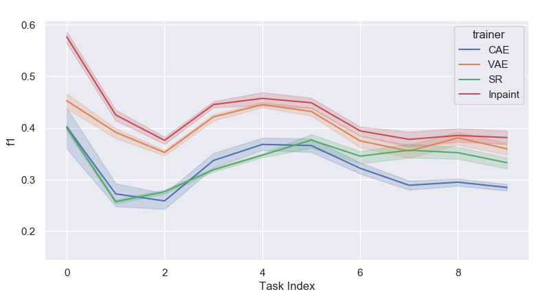
(a) Single Model

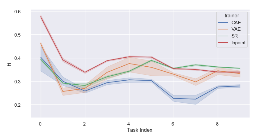
(b) Ideal Replay

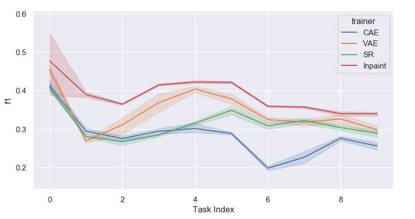
(c) Replay

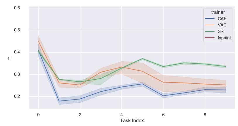
(d) Compressed Replay

Figure 6: Each plot shows the performance for a strategy comparing different architectures in terms of AD performance i.e. Average f1 score. The Average f1 metric is shown on axis y, and the index of the current training task is shown on axis x.

Regarding the AD results, it should be kept in mind that CAE, VAE, SR, and Inpaint are all reconstruction-based methods, whereas FastFlow is an embedding similarity-based method that uses pre-trained models for feature extraction and is considered state-of-the-art in the field. Embedding similarity-based methods, such as FastFlow, are incapable of acting as Memory Module because they produce only the anomaly map as output and not the reconstructed image. As a result, when we use the Compressed Replay strategy on FastFlow and Inpaint, we use the SR architecture as the Memory Module (which turns out to be the best among the generative models as shown in Section 6.2) and FastFlow and Inpaint as the AD Module.

In Fig. 5 we show the results of AD obtained for a sample with two different architectures VAE and SR. The first image in the row shows the original image, while the second column displays the reconstructed image produced by the model. The third column presents the ground truth for each pixel, which provides a reference for evaluating the accuracy of the reconstructed image. The fourth column displays the anomaly map, which indicates the probability that each pixel is anomalous (i.e., differs significantly from the ground truth). This can help identify areas of the image that may be corrupted. The fifth column shows the predicted class for each pixel, which can provide additional information about the final prediction of the model on what is considered anomalous. Finally, the sixth column presents the portion of the image that contains anomalous parts, highlighting any potential issues with the image. This can help users quickly identify and address any problems with the image.

The final values for AD performance are showed in Table 1 varying strategy and architecture.

In the Single Model (classic setting), FastFlow performs better than the other models, as expected. It is significantly better than the next best model, with a margin of 0.57. However, in the CL setting, FastFlow performs poorly for both the Replay and Ideal Replay strategies. When using the Compressed Replay strategy, FastFlow performs better than the CAE and VAE models, but still worse than SR and Inpaint. Interestingly, when FastFlow is evaluated using the Compressed Replay strategy, it outperforms Replay in terms of AD performance. We can observe that, among the feasible Replay-based strategies, the best combination is Inpaint as AD Module with SR as Memory Module trained according to the Compressed Replay Strategy.

In addition, it should be observed from Table 1 that the fine-tuning strategy appears to have better values in FastFlow than in other models.

In terms of forgetting, as shown in Table 1, FastFlow has a significantly higher forgetting than the other approaches. Instead, in terms of forgetting, SR with Compressed Replay has a very low forgetting.

Fig. 6 presents the results in greater detail, displaying the performance progressively as each task is presented in sequence. The Figure shows four different plots, each representing the performance of a specific strategy. The x-axis of each plot indicates the task ID of the training, while the y-axis represents the value of the chosen metric. Each line in the plot represents a different model. The value at the task $i$ include only the performance on the tasks seen so far.

6.2 Quality of the reconstructed images

Table 2: Summary table about the quality of reconstructed images for different models. For each model and strategy, we report the FID value. Please note that the lower FID, the better the reconstruction is. In round brackets we report also the forgetting value in percentual. Note that for each strategy the best architecture is SR. Moreover, the best strategy results to be Compressed Replay. The best combination is in bold while the best architecture for each strategy is in italic.

	Average FID $\downarrow$
Strategy	CAE	VAE	SR	Inpaint
Single Model	266.52	219.40	125.15	204.29
FT	376.64 (73.65%)	399.44 (91.33%)	244.25 (194.31%)	363.20 (114.41%)
Ideal Replay	216.82 (7.50%)	255.84 (11.93%)	89.53 (7.74%)	192.12 (5.24%)
Replay	227.88 (14.70%)	245.87 (14.54%)	111.87 (40.6%)	181.74 (7.90%)
Compressed Replay	248.42 (20.33%)	316.48 (36.17%)	105.57 (14.66%)	-
Generative Replay	-	405.34 (77.84%)	-	-

(a) Single Model

(b) Ideal Replay

(c) Replay

(d) Compressed Replay

Figure 7: The results show the quality of the constructed images for different continual learning (CL) strategies and architectures. Each plot represents a different CL strategy, and each line represents a different architecture. The y-axis shows the FID metric, and the x-axis shows the index of the current training task. Each value represents the average FID across all tasks seen so far, with a lower value indicating a higher quality of reconstruction. The plots show that the best architecture for each CL strategy is SR, our approach.

Table 2 shows a summary of the results, which corresponds to the average FID on all tasks evaluated at the end of the training. Table 2 also displays the associated percentual forgetting value in round brackets.

Moreover, it is possible to examine average FID on the tasks seen so far in the plots of Fig. 7. For each strategy, the performance of each model is shown, where a lower value means a better quality of the reconstructed image.

From Fig. 7, we can clearly see that the SR model is the best architecture for each strategy considered. For each of the strategies considered, the gap between SR and other architectures is significant. In other words, regardless of the strategy, the SR model is the best for learning a good representation of the original images. Moreover, its output is conditoned by the scaled image and random noise which means a certain level of randomness in output, while in the classic GANs imply a very quickly forgetting [43], that it doesn’t happen in our case. Despite all these aspects, the SR is able to obtain a good representation of the original distribution.
As stated above, Inpaint can’t act as Memory Modules like CAE and VAE because it cannot perform Compressed Replay. However, since Inpaint is a generative model, we can still analyze its reconstruction performance in terms of FID in Table 2 and Fig. 7.

Another interesting fact is that CAE seems to have a more stable trend than VAE in Latent Replay strategy. In fact, it can be observed that while CAE is worse than VAE in Single Model, it obtains better performance for Replay and Compressed Replay.

Among the proposed models VAE is the only one to be applied under the Generative Replay strategy. Results are shown in Table 2 and it can be seen that, as said before, the forgetting is very high.
According to these graphs, the difference between Compressed Replay and Ideal Replay appears to be greater for models CAE and VAE than for SR and Inpaint.
It should be noted that the compression factors for the CAE, VAE, and SR architectures are 6, 196, and 64, respectively.
The only model that allows Generative Replay is VAE, but as seen in 2, the performance degrades very quickly, so it is only shown in the tables and not the plots (the same for fine-tuning).
As a final remark, it can be stated that the SR model allows for a good compression factor while maintaining a very high image quality in memory.

6.3 Results of SR Model

Strategy	epochs	Average FID $\downarrow$	FID Increase % wrt Ideal Replay $\downarrow$
Single Model	30	125.15	-
Ideal Replay	30	89.53 (7.74%)	-
Replay	30	111.87 (40.6%)	24.95%
Compressed Degenerative Replay	30	106.49 (13.58%)	18.94%
Compressed Replay	30	105.57 (14.66%)	17.92%
Single Model	50	82.06	-
Ideal Replay	50	85.27 (11.18%)	-
Replay	50	109.51 (59.41%)	28.43%
Compressed Degenerative Replay	50	97.31 (19.08%)	14.12%
Compressed Replay	50	91.17 (10.88%)	6.92%

Table 3: Comparison of different strategies for training a SR model. The table shows the results for two different values of the number of epochs (30 and 50). The FID score is shown in the third column, with the percentage of forgetting in round brackets. The fourth column shows the increase in performance with respect to the Ideal Replay strategy, in other words more a value is lower and more is close to the optimal. The best results for each number of epochs are highlighted in bold.

As the first study on Super Resolution in the context of Continual Learning, we thoroughly examine how variables such as the number of epochs and the way in which images are saved affect the final performance in terms of the quality of the reconstructed images. This analysis helps us to gain insight into the critical issues facing generative models such as GANs in Continual Learning. Based on this analysis, we conclude that there are at least three critical issues that arise during the training of GANs in CL.

1. The initial quality of the learned distribution is the first critical issue. Based on the number of epochs, we can easily demonstrate that an initial higher quality has a long-term beneficial effect.

2. In classic GANs, we create images only using a random vector for each new task, producing an output image that will be used as input to the model at the new task. However, there will be some perturbation in the final image. These perturbations accumulate in the produced images over time, increasing their distance from the original distribution.

3. The third critical issue is catastrophic forgetting of the model’s weights, which is inherent in all models in the CL setting.

To simplify the explanation we are going to define the following notation:

• $X_{i}$: The original data of the $i$-th Task;

• $O_{i}(X_{i})$: The output produced by SR after training the i-th Task on data $X_{i}$;

• $S_{i}$: The scaled images of the data $X_{i}$;

• $M_{ij}$: The memory about the $j-$th Task after training the $i$-th Task.

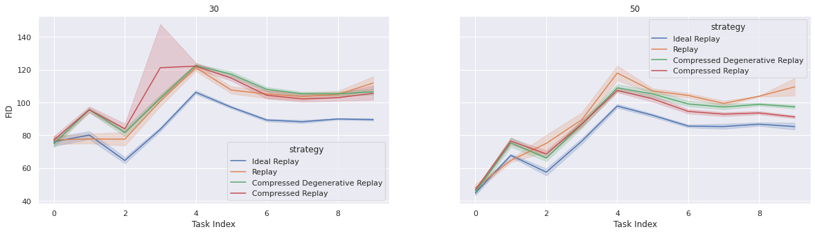
Figure 8: The comparison of the SR model using 30 epochs (left) and 50 epochs (right) with different strategies is shown in the figures. The y-axis shows the FID metric, and the x-axis shows the index of the current training task. It can be observed that the Compressed Replay strategy performs closer to the Ideal Replay strategy (i.e. the optimal performance) when there is an increase in the number of epochs from 30 to 50.

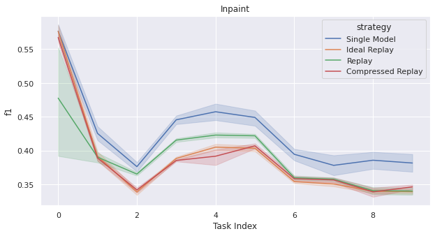
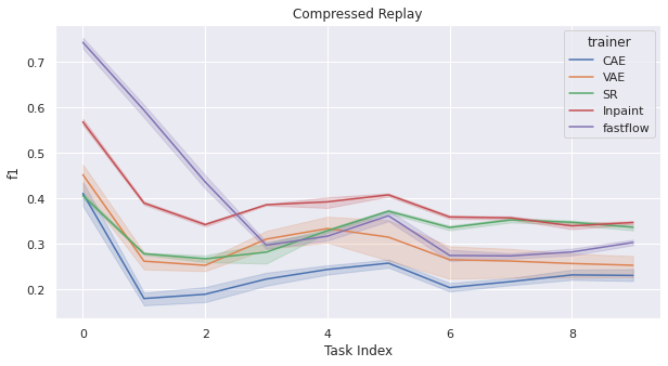
Figure 9: The figure on the left shows the best model using different continual learning (CL) strategies, and the figure on the right shows all models using the Compressed Replay strategy. The y-axis shows the Average f1 metric, and the x-axis shows the index of the current training task.

In Compressed Replay for SR, the scaled image $S_{i}$ is saved in memory $M_{i,i}$ during the $i$-th Task i.e. $M_{i,i}=S_{i}$. Such scaled images will never be changed, they will remain fixed over time or in other terms $M_{i,i}=M_{i+1,i}=\cdots=M_{T,i}$.
Now we define a modified version called Compressed Degenerative Replay that simulates the critical issue (ii) present in GANs, where the images used for an old task during the training of a new task are different from the images used for a previous task. During the $(i+1)-$th Task, we take the images saved during the previous task $M_{i,i}=S_{i}$ and produce the new reconstructed images as $O_{i+1}(S_{i})$. Such images are scaled and saved in memory i.e. $M_{i+1,i}=O_{i+1}(S_{i})$. This is repeated for all the tasks and then we have that for the $i$-th Task the memory change overtime i.e. $M_{i,i}\neq M_{i+1,i}\neq\cdots\neq M_{T,i}$

The difference in results for each strategy based on the number of epochs (30 or 50) can be seen in Table 3 and Fig. 8. Generally, the results obtained using a larger number of epochs (i.e., a better initial learned representation) are better, as expected. For example, the Ideal Replay strategy improves from 95.2 to 89.5 in terms of FID, and the Replay strategy improves from 112 to 109.5. However, the most significant improvement is seen with the Compressed Replay strategy, which drops from 105.5 to 91. In terms of percentage increase compared to Replay, Compressed Replay shows a minor decrease at 50 epochs (7%) compared to 30 epochs (18%). This suggests that the proposed solution performs very close to the upper bound of Ideal Replay, particularly when the initially learned representation is very good (i.e., a higher number of epochs).

Finally, when comparing the Compressed Replay strategy vs Compressed Degenerative Replay strategy, we can see that the positive effect of Compressed Replay vs compressed Degenerative Replay increases with the number of epochs. Indeed, with 50 epochs, Compressed Replay has a 7% increase over Ideal Replay, while Compressed Degenerative Replay has a 14% increase. Furthermore, the percentage increase in comparison to the Ideal Replay for Compressed Degenerative Replay is lower for 50 epochs (14% instead of 18%). This means that using more epochs and Compressed Replay instead of Replay or compressed Degenerative Replay allows you to get closer to the Ideal Replay, which uses the original distribution in memory.
However, while Compressed Degenerative Replay is inferior to Compressed Replay, the table shows that Compressed Degenerative Replay with 50 epochs is superior to Compressed Replay with 30 epochs. This means that the main factor is the number of epochs i.e. the initial quality of the learned representation.

7 Conclusions

In this research, we propose a framework for performing anomaly detection in a setting where the model is continually learning new tasks. Our approach combines a Memory module, which stores information from previous tasks, and an Anomaly Detection module, which identifies anomalies in new data. By using these modules together, our approach can detect anomalies at the pixel level in new image classes without forgetting how to identify anomalies in previously learned classes. To the best of our knowledge, this is the first time that a method using a Super Resolution module to enable Compressed Replay has been proposed for use in continual learning. We also suggest a real-world benchmark dataset specifically designed for evaluating the performance of anomaly detection approaches in a continual learning setting.

There are several potential future developments. Application and evaluation of other models considered state-of-the-art in Anomaly Detection in the CL setting should be a research direction. Furthermore, some of these models could be modified to produce better results in the case of Anomaly Detection for Continual Learning. While the MVTec Dataset is an excellent benchmark for Anomaly Detection, other datasets could be used to confirm the models’ efficacy. Furthermore, a follow-up study on the SR problem should be carried out, analyzing models closer to the state of the art and using a more complex dataset to validate their efficacy in the Continual Learning setting.

References

- [1] F. Wiewel, B. Yang, Continual learning for anomaly detection with variational autoencoder, in: ICASSP 2019 - 2019 IEEE International Conference on Acoustics, Speech and Signal Processing (ICASSP), 2019, pp. 3837–3841. doi:10.1109/ICASSP.2019.8682702.
-
[2]
G. M. van de Ven, A. S. Tolias, Three
scenarios for continual learning, CoRR abs/1904.07734 (2019).
arXiv:1904.07734.
URL http://arxiv.org/abs/1904.07734 - [3] M. De Lange, R. Aljundi, M. Masana, S. Parisot, X. Jia, A. Leonardis, G. Slabaugh, T. Tuytelaars, A continual learning survey: Defying forgetting in classification tasks, IEEE transactions on pattern analysis and machine intelligence 44 (7) (2021) 3366–3385.
-
[4]
A. ROBINS, Catastrophic
forgetting, rehearsal and pseudorehearsal, Connection Science 7 (2) (1995)
123–146.
arXiv:https://doi.org/10.1080/09540099550039318, doi:10.1080/09540099550039318.
URL https://doi.org/10.1080/09540099550039318 -
[5]
G. Merlin, V. Lomonaco, A. Cossu, A. Carta, D. Bacciu,
Practical recommendations for
replay-based continual learning methods.
doi:10.48550/ARXIV.2203.10317.
URL https://arxiv.org/abs/2203.10317 - [6] P. Isola, J.-Y. Zhu, T. Zhou, A. A. Efros, Image-to-image translation with conditional adversarial networks, in: Proceedings of the IEEE conference on computer vision and pattern recognition, 2017, pp. 1125–1134.
- [7] J. Yang, R. Xu, Z. Qi, Y. Shi, Visual anomaly detection for images: A systematic survey, Procedia Computer Science 199 (2022) 471–478.
- [8] P. Bergmann, M. Fauser, D. Sattlegger, C. Steger, Mvtec ad — a comprehensive real-world dataset for unsupervised anomaly detection, in: 2019 IEEE/CVF Conference on Computer Vision and Pattern Recognition (CVPR), 2019, pp. 9584–9592. doi:10.1109/CVPR.2019.00982.
- [9] H. Shin, J. K. Lee, J. Kim, J. Kim, Continual learning with deep generative replay, Advances in neural information processing systems 30 (2017).
- [10] D. Rolnick, A. Ahuja, J. Schwarz, T. Lillicrap, G. Wayne, Experience replay for continual learning, Advances in Neural Information Processing Systems 32 (2019).
- [11] X. Chen, J. Jiang, Z. Li, H. Qi, Q. Li, J. Liu, L. Zheng, M. Liu, Y. Deng, An online continual object detector on vhr remote sensing images with class imbalance, Engineering Applications of Artificial Intelligence 117 (2023) 105549.
- [12] J. Pomponi, S. Scardapane, V. Lomonaco, A. Uncini, Efficient continual learning in neural networks with embedding regularization, Neurocomputing 397 (2020) 139–148.
- [13] J. Ramapuram, M. Gregorova, A. Kalousis, Lifelong generative modeling, Neurocomputing 404 (2020) 381–400.
- [14] Y.-n. Han, J.-w. Liu, Online continual learning via the meta-learning update with multi-scale knowledge distillation and data augmentation, Engineering Applications of Artificial Intelligence 113 (2022) 104966.
- [15] G. Sokar, D. C. Mocanu, M. Pechenizkiy, Spacenet: Make free space for continual learning, Neurocomputing 439 (2021) 1–11.
- [16] A. Mallya, D. Davis, S. Lazebnik, Piggyback: Adapting a single network to multiple tasks by learning to mask weights, in: Proceedings of the European Conference on Computer Vision (ECCV), 2018, pp. 67–82.
-
[17]
Q. Yang, F. Feng, R. Chan, A benchmark
and empirical analysis for replay strategies in continual learning (2022).
doi:10.48550/ARXIV.2208.02660.
URL https://arxiv.org/abs/2208.02660 - [18] L. Pellegrini, G. Graffieti, V. Lomonaco, D. Maltoni, Latent replay for real-time continual learning, in: 2020 IEEE/RSJ International Conference on Intelligent Robots and Systems (IROS), IEEE, 2020, pp. 10203–10209.
- [19] P. Buzzega, M. Boschini, A. Porrello, S. Calderara, Rethinking experience replay: a bag of tricks for continual learning, in: 2020 25th International Conference on Pattern Recognition (ICPR), IEEE, 2021, pp. 2180–2187.
- [20] C. D. Kim, J. Jeong, G. Kim, Imbalanced continual learning with partitioning reservoir sampling, in: European Conference on Computer Vision, Springer, 2020, pp. 411–428.
- [21] A. Chaudhry, M. Rohrbach, M. Elhoseiny, T. Ajanthan, P. K. Dokania, P. H. Torr, M. Ranzato, On tiny episodic memories in continual learning, arXiv preprint arXiv:1902.10486 (2019).
- [22] O. Ostapenko, T. Lesort, P. Rodríguez, M. R. Arefin, A. Douillard, I. Rish, L. Charlin, Foundational models for continual learning: An empirical study of latent replay, arXiv preprint arXiv:2205.00329 (2022).
- [23] T. L. Hayes, K. Kafle, R. Shrestha, M. Acharya, C. Kanan, Remind your neural network to prevent catastrophic forgetting, in: European Conference on Computer Vision, Springer, 2020, pp. 466–483.
- [24] A. Iscen, J. Zhang, S. Lazebnik, C. Schmid, Memory-efficient incremental learning through feature adaptation, in: European conference on computer vision, Springer, 2020, pp. 699–715.
- [25] A. Ayub, A. R. Wagner, Storing encoded episodes as concepts for continual learning, arXiv preprint arXiv:2007.06637 (2020).
- [26] L. Caccia, E. Belilovsky, M. Caccia, J. Pineau, Online learned continual compression with adaptive quantization modules, in: International conference on machine learning, PMLR, 2020, pp. 1240–1250.
- [27] S. K. Amalapuram, A. Tadwai, R. Vinta, S. S. Channappayya, B. R. Tamma, Continual learning for anomaly based network intrusion detection, in: 2022 14th International Conference on COMmunication Systems & NETworkS (COMSNETS), IEEE, 2022, pp. 497–505.
- [28] B. Maschler, T. T. H. Pham, M. Weyrich, Regularization-based continual learning for anomaly detection in discrete manufacturing, Procedia CIRP 104 (2021) 452–457.
-
[29]
A.-S. Collin, C. De Vleeschouwer,
Improved anomaly detection by
training an autoencoder with skip connections on images corrupted with
stain-shaped noise (2020).
doi:10.48550/ARXIV.2008.12977.
URL https://arxiv.org/abs/2008.12977 -
[30]
V. Zavrtanik, M. Kristan, D. Skočaj,