Accelerating relaxation in Markovian open quantum systems through quantum reset processes

Abstract

The divergent timescales of slow relaxation processes are obstacles to the study of stationary state properties and the functionalization of some systems like steady state heat engines, both in classical and quantum systems. Thus the shortening of the relaxation time scale would be desirable in many cases. Here we claim that using quantum reset, a common and important operation in quantum computation, the relaxation dynamics of general Markovian open quantum systems with arbitrary initial states is able to be accelerated significantly through a simple protocol. This faster relaxation induced by the reset protocol is reminiscent of the quantum Mpemba effect. The reset protocol we proposed is applied to a two-state quantum systems to illustrate our theory, which may characterize a single qubit or a spin. Furthermore, our new strategy to accelerate relaxations may also be applied to closed quantum systems or even some non-Markovian open quantum systems.

Introduction.—Relaxation processes, typically conducing to stationary states, are ubiquitous in both quantum and classical systems and are crucial research topics in non-equilibrium statistical physics. Intriguingly, relaxation processes are varied and nontrivial even within the framework of Markovian dynamics Shiraishi and Saito (2019), such as non-monotonic relaxations known as the Mpemba effect Lu and Raz (2017); Klich et al. (2019); Santos and Prados (2020); Kumar and Bechhoefer (2020); Gal and Raz (2020); Busiello et al. (2021), slow relaxations in glassy systems Toninelli et al. (2004), and the anomalously far from equilibrium relaxation in the Ising anti-ferromagnetic chain system Teza et al. (2022). However, in many cases faster paces to stationary states are preferred, when the stationary states are desired for further study or use Carollo et al. (2021). For instance, (periodic) steady states could serve as the functional states of some classical or quantum heat engines, in which they can output power Brandner et al. (2017); Um et al. (2022); Pietzonka and Seifert (2018). In addition, fast relaxation is beneficial for control of quantum systems, quantum computing and the preparations of quantum states Dann et al. (2019).

Stochastic reset, a dynamical protocol to stop a stochastic process randomly and start it anew, is of wide interest in the past decade Evans and Majumdar (2011); Gupta et al. (2014); Roldán et al. (2016); Reuveni (2016); Belan (2018); Chechkin and Sokolov (2018); Pal et al. (2019); Gupta and Jayannavar (2022); De Bruyne et al. (2020); Perfetto et al. (2021); Miron and Reuveni (2021); De Bruyne et al. (2022); Ruoyu Yin (2022); Busiello et al. (2021). It was found that reset can benefit dynamical processes in classical systems, such as reducing the mean first passage time of diffusion processes Evans and Majumdar (2011) and accelerating the relaxation processes Busiello et al. (2021). Recently, there are also a surge of works in quantum reset processes, including studies of the reset’s effect on closed qunatum dynamics Mukherjee et al. (2018); Perfetto et al. (2021); Ruoyu Yin (2022) and studies on the change of stationary state properties or thermodynamics of open quantum systems due to reset Rose et al. (2018); Perfetto et al. (2022). However, the effect of reset on the relaxation dynamics of open quantum systems remains to be explored. Quantum reset is an important and common operation for the quantum state preparation, which is a key step in quantum computation Buffoni et al. (2022). For instance, at the beginning of a quantum computation process, initialization of qubits to the computational state $|00...0\rangle$ is realized by the reset operation. Therefore it’s natural to ask whether this crucial operation in quantum system could serve as an approach to benefit quantum dynamics as it does in classical systems.

Here in this letter, we connect the quantum reset protocol with the acceleration of relaxations to stationarity in open quantum systems described by the Markovian Lindblad master equations. We show that quantum reset is able to drive systems with arbitrary initial states to accelerated approaches where they can reach stationary states significantly faster. The acceleration is realized by a simple reset protocol adding reset to the system for a given time and closing the reset after that, which would be further discussed later.

Spectral analysis of the Markovian open quantum dynamics.—We are considering open quantum systems in a Hilbert space $\mathcal{H}$ of dimension $d$, whose dynamics in the interaction picture are described by the Lindblad-Gorini-Kossakowski-Sudarshan (LGKS) master equation

$$\frac{d\rho}{dt}=\mathcal{L}(\rho),$$ (1)

where

$$\mathcal{L}(\rho)\equiv-i[H,\rho]+\sum_{i}\left[J_{i}\rho J_{i}^{\dagger}-\frac{1}{2}\{J_{i}^{\dagger}J_{i},\rho\}\right]$$ (2)

is the Lindbladian. It preserves the trace and Hermiticity {$\text{Tr}[\mathcal{L}(X)]=0,\ (\mathcal{L}(X))^{\dagger}=\mathcal{L}(X^{\text{$\dagger$}}),\ \forall X$}, which assures the completely positive dynamics of the density operator $\rho$. Here $H$ is the Hamiltonian of the system and the jump operators $J_{i}$ describe the dissipation effect due to environment, mediating the system-bath interaction. For closed quantum systems, the jump operators turn to be zero. The evolution of the system can also be described in terms of the eigenvalues and eigenmatrices of $\mathcal{L}$ since it acts linearly on the density matrix. We denote the eigenvalues of $\mathcal{L}$ by $\lambda_{k}$ and order them such that 0$\geq$Re($\lambda_{k}$)$\geq\text{Re}(\lambda_{k+1}).$ Assuming that the generator $\mathcal{L}$ is able to be diagonalized, the right eigenmatrices $R_{k}$ and left eigenmatrices $L_{k}$ can be found by

$$\mathcal{L}(R_{k})=\lambda_{k}R_{k},$$

and

$$\mathcal{L^{\dagger}}(L_{k})=\lambda_{k}^{\star}L_{k},\ k=1,..,d^{2}$$

respectively. They are normalized as

$$\text{Tr}(L_{k}^{\dagger}R_{h})=\delta_{kh}.$$ (3)

Note that the dual operator $\mathcal{L}^{\dagger}$ implementing the evolution of observables is defined as:

$$\mathcal{L}^{\dagger}(O)=i[H,O]+\sum_{i}\left[J_{i}OJ_{i}^{\dagger}-\frac{1}{2}\{J_{i}^{\dagger}J_{i},O\}\right].$$ (4)

Then, given an initial state $\rho_{0}$, the system state at time $t$ can be expressed as

$$\rho(t)=e^{t\mathcal{L}}[\rho_{0}]=\rho_{ss}+\sum_{k=2}^{d^{2}}e^{\lambda_{k}t}\text{Tr}(L_{k}^{\dagger}\rho_{0})R_{k},$$ (5)

in which the unique stationary state of the open quantum system $\rho_{ss}$ is given by

$$\rho_{ss}=\lim_{t\rightarrow\infty}\rho(t)=R_{1},$$ (6)

if assuming the first eigenvalue $\lambda_{1}=0$ is non-degenerate. We further assume that the second eigenvalue $\lambda_{2}$ is real and unique Carollo et al. (2021), so that there is a spectral gap, then for long time one has

$$||\rho(t)-\rho_{ss}||\sim\exp\left(\lambda_{2}t\right).$$

In this case, for the system with a general initial state, the timescale for relaxation is determined by

$$\tau=\frac{1}{|\lambda_{2}|},$$ (7)

when the slowest decaying mode $e^{t\lambda_{2}}R_{2}$ is excited.

Reset protocol to accelerate relaxation processes.—To prevent the slowest decaying mode of the quantum systems with general initial states from being excited, we introduce a quantum reset dynamics. We let initial states evolve under this quantum reset dynamics for a given time $t_{s}$, during which reset of the system to a given reset state $|\delta\rangle$ occurs randomly at times distributed exponentially with constant rate $r$. After $t_{s},$ the reset is closed and the system follows the reset-free dynamics according to the original Lindbladian. Next, we would like to show that this quantum reset process can eliminate the overlaps of the initial state with the slowest dynamical mode by appropriately setting the reset time $t_{s}$, i.e.,

$$\text{Tr[$L_{2}^{\dagger}$$\rho^{r}(t_{s})$]}=0$$ (8)

is realized. Here

$$\rho^{r}(t_{s})=e^{t_{s}\mathcal{L}_{r}}\rho_{0}$$

and $\mathcal{L}_{r}$ is the generalized Lindblad operator with reset, as we will see below. The quantum reset dynamics can be simply constructed by adding jump operators

$$J_{i}^{r}=\sqrt{r}|\delta\rangle\langle\phi_{i}|$$ (9)

to the Lindbladian (2). Here $|\phi_{i}\rangle$ form an auxiliary complete orthonormal basis. This modification gives rise to the generalized Lindblad operator as

$$\mathcal{L}_{r}(\rho)=\mathcal{L}(\rho)+r\text{Tr}(\rho)|\delta\rangle\langle\delta|-r\rho.$$ (10)

The eigenvalue equations of this new operator are Rose et al. (2018)

$$\mathcal{L}_{r}(R_{i})=(\lambda_{i}-r)R_{i},\ i\in\{2,...,d^{2}\},$$ (11)

That is, the eigenmatrices are unchanged and the eigenvalues are all shifted down by a value $r$ compared to the original Lindbladian. Then, acting the time-evolution operator generated by this generalized Lindblad operator on the eigenvalue-expanded form of the initial state

$$\rho_{0}=\rho_{ss}+\sum_{k=2}^{d^{2}}\text{Tr}(L_{k}^{\dagger}\rho_{0})R_{k}$$ (12)

results in

$$\rho^{r}(t)= e^{t\mathcal{L}_{r}}\rho_{0}$$

$$= e^{t\mathcal{L}_{r}}\rho_{ss}+\sum_{k=2}^{d^{2}}\text{Tr}(L_{k}^{\dagger}\rho_{0})e^{(\lambda_{k}-r)t}R_{k}.$$ (13)

To get the detailed form of the first term, note that the stationary state under reset dynamics has been determined by Garrahan as

$$\rho_{ss}^{r}=\lim_{t\rightarrow\infty}\rho^{r}(t)=\rho_{ss}+\sum_{k=2}^{d^{2}}\frac{r\langle\delta|L_{k}^{\dagger}|\delta\rangle}{r-\lambda_{k}}R_{k},$$ (14)

and the stationary state has the property that

$$e^{t\mathcal{L}_{r}}\rho_{ss}^{r}=\rho_{ss}^{r}.$$ (15)

Thus, acting $e^{t\mathcal{L}_{r}}$ on both sides of the Eq.(14) and combining Eq.(15) bring about

$$e^{t\mathcal{L}_{r}}\rho_{ss}+\sum_{k=2}^{d^{2}}\frac{r\langle\delta|L_{k}^{\dagger}|\delta\rangle}{r-\lambda_{k}}e^{(\lambda_{k}-r)t}R_{k}$$

$$=\rho_{ss}+\sum_{k=2}^{d^{2}}\frac{r\langle\delta|L_{k}^{\dagger}|\delta\rangle}{r-\lambda_{k}}R_{k}$$ . (16)

Combining these equations one finds

$$\rho^{r}(t)= e^{t\mathcal{L}_{r}}\rho_{ss}+\sum_{k=2}^{d^{2}}\text{Tr}(L_{k}^{\dagger}\rho_{0})e^{(\lambda_{k}-r)t}R_{k}$$

$$= \rho_{ss}+\sum_{k}a_{k}(t)e^{\lambda_{k}t}R_{k},$$ (17)

with the time-dependent expansion coefficients $a_{k}(t)$ being defined as

$$a_{k}(t)\equiv\left[\text{Tr}(L_{k}^{\dagger}\rho_{0})-\frac{r\langle\delta|L_{k}^{\dagger}|\delta\rangle}{r-\lambda_{k}}\right]e^{-rt}+\frac{r\langle\delta|L_{k}^{\dagger}|\delta\rangle}{r-\lambda_{k}}e^{-\lambda_{k}t}.$$ (18)

To fulfill the condition $\text{Tr[$L_{2}^{\dagger}$$\rho^{r}(t_{s})$]}=0$, one let

$$a_{2}(t_{s})=0.$$ (19)

Then one can obtain the resetting time $t_{s}$ through the equation

$$\left[\text{Tr}(L_{2}^{\dagger}\rho_{0})-\frac{r\langle\delta|L_{2}^{\dagger}|\delta\rangle}{r-\lambda_{2}}\right]e^{-rt_{s}}+\frac{r\langle\delta|L_{2}^{\dagger}|\delta\rangle}{r-\lambda_{2}}e^{-\lambda_{2}t_{s}}=0,$$ (20)

whose solution is simply given by

$$t_{s}(r)=\frac{1}{r-\lambda_{2}}\ln\left[1-\frac{\text{Tr}(L_{2}^{\dagger}\rho_{0})(r-\lambda_{2})}{r\langle\delta|L_{2}^{\dagger}|\delta\rangle}\right].$$ (21)

For an arbitrary initial state $\rho_{0}$ which may be a mixed state, one can appropriately choose the reset state $|\delta\rangle$ so that $t_{s}(r)\geq 0$, leading to an exponentially fast pace to stationarity. The whole dynamics of this open quantum system is given by

$$\rho^{r}(t)= \rho_{ss}+\sum_{k}a_{k}(t)e^{\lambda_{k}t}\Theta(t_{s}-t)R_{k}$$

$$+\sum_{k}a_{k}(t_{s})e^{\lambda_{k}t}\Theta(t-t_{s})R_{k}.$$ (22)

Application to a two-level quantum system.—To illustrate our theory, we take a two-level quantum system as an example, which may represent a single qubit or a spin. For brevity, we set the ground state energy $E_{0}=0$ and the excited state energy $E_{1}=E$, then the total Hamiltonian may be

$$H=E|1\rangle\langle 1|+\Omega(|0\rangle\langle 1|+|1\rangle\langle 0|)\text{,}$$ (23)

where $\Omega$ is the frequency of intrinsic transition between state $|1\rangle$ and state $|0\rangle.$ The Lindblad jump operators describing the dissipation effect due to coupling to the environment are given by

$$J_{0} =|1\rangle\langle 0|=\sigma_{+},$$ (24)

$$J_{1} =|0\rangle\langle 1|=\sigma_{-},$$ (25)

then the original Lindblad master equation governing the dynamics of the reduced density matrix $\rho(t)$ of the system reads

$$\frac{d\rho(t)}{dt}= -i[H,\rho]+\Gamma_{0}\left(J_{0}\rho J_{1}-\frac{1}{2}\{J_{0}J_{1},\rho\}\right)$$

$$+\Gamma_{1}\left(J_{1}\rho J_{0}-\frac{1}{2}\{J_{1}J_{0},\rho\}\right),$$ (26)

where $\Gamma_{0,1}$ are the transition rates from state $|0\rangle$ to state $|1\rangle$ or converse. Assuming the transition rates obey the detailed balance condition $\Gamma_{0}e^{-\beta_{\text{env}}E_{0}}=\Gamma_{1}e^{-\beta_{\text{env}}E_{1}}$, i.e.,

$$\Gamma_{0}=\Gamma_{1}e^{-\beta_{\text{env}}E},$$

then this two-level system with any initial condition $\rho_{0}$ would evolve into a unique equilibrium stationary state $\rho_{\text{eq}}$ depending on the environment temperature $T=1/\beta_{\text{env}}$, given by

$$\hat{\rho}_{eq}=\frac{e^{-\beta_{\text{env}}H}}{\text{Tr}(e^{-\beta_{\text{env}}H})}.$$ (27)

To study the relaxation dynamics, we consider a general initial state as

$$\hat{\rho}_{0} =\left(\begin{array}[]{cc}\frac{1}{1+e^{-\beta_{0}E}}&ke^{i\phi}\\ ke^{-i\phi}&\frac{e^{-\beta_{0}E}}{1+e^{-\beta_{0}E}}\end{array}\right),$$ (30)

$$0\leq k \leq\frac{\sqrt{e^{\beta_{0}E}}}{e^{\beta_{0}E}+1},\quad 0\leq\phi\leq 2\pi,$$ (31)

where the off-diagonal terms $ke^{\pm i\phi}$ quantify the amount of coherence in the initial state. Firstly, let’s consider the simple case when there is no intrinsic transitions ($\Omega=0$). In this case, the two-state system will finally converge to a unique Gibbs state $\hat{\rho}_{eq}$ whose off-diagonal terms vanish. Thus the corresponding relaxation process can be regarded as a decoherence process. All the eigenmatrices and eigenvalues of the Lindbladian can be computed exactly, which we list in the Appendix B. We choose the ground state $|0\rangle\langle 0|$ as the reset state, which may be more friendly for experimental realizations. Then using Eq. (22), the whole dynamics of this simple system under our reset protocol can be obtained. To quantify the distance between the state $\rho(t)$ and the final stationary state $\rho_{ss}$, we utilize a common choice of the distance measure in quantum systems, the trace distance

$$D[\rho(t)|\rho_{ss}]:=\frac{1}{2}\text{Tr$\lvert\rho(t)-\rho_{ss}\rvert$},$$ (32)

where $|A|:=\sqrt{A^{\dagger}A}$. Equipped with this distance measure, we fix all dynamical parameters and plot the trace distances between $\rho(t)$ and $\rho_{\text{eq}}$ of this two-state system as the function of time $t$ with different resetting rate $r$, as shown in Figure 1 (a). In the presence of reset protocol, the system is initialized at $\beta_{0}=2.0$, $k=0.32$ and $\phi=1$. The system without reset is initially at $\beta_{0}=3.0,$ $k=0.21$ and $\phi=1$. The environment is set to be at a lower temperature $\beta_{\text{env}}=4.0$, thus the system without reset is initially closer to the target stationary state, compared to the system imposed on the reset protocol. Remarkably, relaxation processes with reset protocol are significantly faster than the free relaxation process without reset, even resulting in the emergence of a anomalous relaxation phenomenon which is similar to Mpemba effect. That is, the systems which are initially farther from the stationary state reach the stationarity sooner. We also plot the critical time $t_{s}$ to close the reset as a function of the resetting $r$ in Figure 1 (b), where $t_{s}$ is shown to be a decreasing function of $r$ with other parameter fixed. This implies that the reset protocol with larger resetting rate $r$ leads to faster relaxation of open quantum systems.

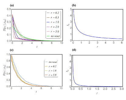
Figure 1: Relaxation dynamics of the two-state system. (a)Distances between $\rho(t)$ and $\rho_{\text{eq}}$ as the function of time $t$ with different resetting rate $r$. (b)The critical time $t_{s}$ as a function of the resetting rate $r$. The parameters are chosen as $\beta_{0}=2.0$, $k=0.32$ and $\phi=1$ with reset protocol and $\beta_{0}=3.0,$ $k=0.21$ and $\phi=1$ without reset.

Note that when there are intrinsic transitions ($\Omega\neq 0$), our reset protocol can still take effects. In Figure 1 (c) we show the effect of our reset protocol on relaxation dynamics when $\Omega=2$, where the relaxation processes of open quantum systems are still accelerated.

The choice of reset state in our protocol is also of interest. To accelerate quantum relaxation through our protocol, the reset state should be chosen to guarantee that the relation $t_{s}(r)\geq 0$ holds. For this two-state system, the expression of $t_{s}$ is given by

$$t_{s}=\frac{\ln\left[1+\frac{\Gamma_{1}k_{\text{tot}}}{r}\left(\frac{1}{\Gamma_{0}+\Gamma_{1}e^{(\beta_{0}-\beta_{\text{env}})E}}-\frac{1}{\Gamma_{0}+\Gamma_{1}}\right)\right]}{k_{\text{tot}}},$$ (33)

where the total transition rate $k_{\text{tot}}=r+\Gamma_{0}+\Gamma_{1}$. One can readily find that when the initial temperature $\beta_{0}<\beta_{\text{env}}$, i.e., the relaxation process corresponds to “cooling the system”, the ground state $|0\rangle\langle 0|$ can always act as an efficacious reset state whatever the resetting rate $r$ is. In contrast, when $\beta_{0}>\beta_{\text{env}}$, reset of the system to the ground state wouldn’t accelerate its relaxation, and one should have to choose the excited state $|1\rangle\langle 1|$ as the reset state.

Concluding remarks.—In conclusion, we propose a new paradigm to accelerate relaxations in open quantum systems through quantum reset processes for general initial states. The reset protocol claimed here is quite convenient to implement, one should just close the reset after a given time $t_{s}$, which can be tuned by the resetting rate $r$. Note that our reset protocol could also be applied to closed quantum system (see Appendix B for details), or even be applicable to some non-Markovian open quantum systems and non-Hermitian open quantum systems, once their dynamics can be described by some linear dynamical equations. There are still some limitations of our reset protocol, for example, when the spectral gap of the dynamical generator is small, this protocol may not accelerate the relaxation process significantly.

An interesting but challenging open problem is to generalize of our work to the case where the slowest decaying modes of the dynamical generator form a complex conjugate pair Kochsiek et al. (2022)

$$\rho(t)=\rho_{ss}+e^{\lambda_{2}t}\text{Tr}(L_{2}^{\dagger}\rho_{0})R_{2}+e^{\lambda_{2}^{\dagger}t}\text{Tr}(L_{2}\rho_{0})R_{2}^{\dagger}+...,$$ (34)

where our reset protocol cannot eliminate two slowest modes simultaneously to realize acceleration.

This work is supported by MOST(2018YFA0208702).

Appendix

Appendix A Spectral analysis of the two-state model

The Eq. (26) can be rewritten as a matrix equation for the vector $\vec{\rho}(t)=[\rho_{00}(t),\rho_{01}(t),\rho_{10}(t),\rho_{11}(t)]^{T}$:

$$\frac{d\vec{\rho}(t)}{dt}=L\vec{\rho}(t),$$ (35)

where $L$ is a $4\times 4$ Liouvillian matrix in the Fock-Liouvillian space, taking the form as

$$L=\left(\begin{array}[]{cccc}-\Gamma_{0}&-i\Omega&i\Omega&\Gamma_{1}\\ -i\Omega&-iE-\frac{\Gamma_{0}+\Gamma_{1}}{2}&0&i\Omega\\ i\Omega&0&iE-\frac{\Gamma_{0}+\Gamma_{1}}{2}&-i\Omega\\ \Gamma_{0}&i\Omega&-i\Omega&-\Gamma_{1}\end{array}\right).$$ (36)

In the simple case $\Omega=0$, the right eigenvalues and eigenvectors ot the matrix $L$ are given by

$$\lambda_{1} =0,\ \vec{R}_{1}=(\Gamma_{1},0,0,\Gamma_{0})^{\text{T}}$$

$$\lambda_{2} =-\Gamma_{0}-\Gamma_{1},\ \vec{R}_{2}=(-1,0,0,1)^{\text{T}}$$

$$\lambda_{3} =\frac{1}{2}(-2i-\Gamma_{0}-\Gamma_{1}),\ \vec{R}_{3}=(0,1,0,0)^{\text{T}}$$

$$\lambda_{4} =\frac{1}{2}(2i-\Gamma_{0}-\Gamma_{1}),\ \vec{R}_{4}=(0,0,1,0)^{\text{T}}$$ (37)

Likewise, the left eigenvalues and eigenvectors are given by

$$\lambda_{1}^{\star} =0,\ \vec{R}_{1}=(1,0,0,1)^{\text{T}}$$

$$\lambda_{2}^{\star} =-\Gamma_{0}-\Gamma_{1},\ \vec{R}_{2}=(-\Gamma_{0},0,0,\Gamma_{1})^{\text{T}}$$

$$\lambda_{3}^{\star} =\frac{1}{2}(2i-\Gamma_{0}-\Gamma_{1}),\ \vec{R}_{3}=(0,1,0,0)^{\text{T}}$$

$$\lambda_{4}^{\star} =\frac{1}{2}(-2i-\Gamma_{0}-\Gamma_{1}),\ \vec{R}_{4}=(0,0,1,0)^{\text{T}}.$$ (38)

Then, by Eq.(21) in the main text, the expression for the critical time $t_{s}$ is given by

$$t_{s}=\frac{\ln\left[1+\frac{\Gamma_{1}(r+\Gamma_{0}+\Gamma_{1})\left(\frac{1}{\Gamma_{0}+\Gamma_{0}e^{\beta_{0}E}}-\frac{1}{\Gamma_{0}+\Gamma_{1}}\right)}{r}\right]}{r+\Gamma_{0}+\Gamma_{1}},$$ (39)

from which one can see that the critical time wouldn’t be affected by the coherence terms of the initial state.

Appendix B Application of the reset protocol to closed quantum systems

For a closed quantum system whose dynamics is described by the von-Neumann equation $\dot{\rho}(t)=-i[H,\rho(t)]\equiv L\rho(t),$ it’s also convenient to reconsider the time evolution of the density matrix in the Fock-Liouville space Schmolke and Lutz (2022) as

$$\text{$\frac{d\vec{\rho}(t)}{dt}$}=\hat{L}\vec{\rho}(t),$$ (40)

with $\hat{L}$ being the Liouville superoperator. The system is in a $d$ dimensional Hilbert space, so that $\hat{L}$ is a $d\times d$ matrix. After incorporating the effect of quantum reset, the modified dynamics of the density matrix $\vec{\rho}_{r}(t)$ with quantum reset is simply given by

$$\frac{d\vec{\rho}_{r}(t)}{dt}=\left(\hat{L}-r\hat{I}\right)\vec{\rho}_{r}(t)+r\vec{\Delta},$$ (41)

where $\hat{I}$ is the identity matrix and $\vec{\Delta}$ is a column vector with all but one of its entries being zeros. The only one elements being $1$ corresponds to the pure resetting state $|\delta\rangle\langle\delta|$. The solution to Eq.(41) is formally given by

$$\vec{\rho}_{r}(t)=e^{-rt}e^{\hat{L}t}\vec{\rho}_{r}(0)+\int_{0}^{t}re^{-r\tau}e^{\hat{L}\tau}\vec{\Delta}d\tau,$$ (42)

or in the original Hilbert space as Mukherjee et al. (2018)

$$\rho_{r}(t)=e^{-rt}e^{iHt}\rho_{r}(t)e^{-iHt}+\int_{0}^{t}re^{-r\tau}e^{iH\tau}\Delta e^{-iH\tau}d\tau.$$ (43)

Assuming that there is a unique stationary state $\vec{\rho}_{st}$, then the eigenvalues of $\hat{L}$ satisfy $0=\mu_{1}>\text{Re}(\mu_{2})\geq\text{Re}(\mu_{3})\geq...\geq\text{Re}(\mu_{d^{2}})$, and the corresponding right eigenvectors are $r_{1}=\vec{\rho}_{st},\ r_{2},...,\ r_{d^{2}}$. From completeness relation, the initial state $\vec{\rho}_{r}(0)$ and the reset state $\vec{\Delta}$ can be expressed as

$$\vec{\rho}_{r}(0) =\vec{\rho}_{st}+\sum_{k=2}^{d^{2}}a_{k}r_{k}$$

$$\vec{\Delta} =\vec{\rho}_{st}+\sum_{k=2}^{d^{2}}d_{k}r_{k}.$$ (44)

Plugging the above formula into Eq.(42) and using the relation $e^{\hat{L}t}r_{k}=e^{\mu_{k}t}r_{k}$ lead to

$$\vec{\rho}_{r}(t)= \vec{\rho}_{st}+\sum_{k=2}^{d^{2}}\left[\frac{rd_{k}}{r-\mu_{k}}e^{-\mu_{k}t}+\left(a_{k}-\frac{rd_{k}}{r-\mu_{k}}e^{-rt}\right)\right]r_{k}e^{\mu_{k}t}$$

$$\equiv \vec{\rho}_{st}+\sum_{k=2}^{d^{2}}a_{k}(t)e^{\mu_{k}t}r_{k},$$ (45)

Setting the second modified coefficient $a_{2}(t_{c})=0$ gives rise to the expression of critical time

$$t_{c}=\frac{1}{r-\mu_{2}}\ln\left[1-\frac{a_{2}(r-\mu_{2})}{rd_{2}}\right],$$ (46)

at which the reset is closed (we have assumed that $\mu_{2}$ is real). Therefore, it has been demonstrated that our reset protocol can be imposed on closed quantum systems as well.

Furthermore, our reset protocol may even be applied to some non-Markovian or non-Hermitian open quantum systems, since the reduced dynamics of these systems could also be described by a linear differential equation Du et al. (2022); Carollo et al. (2021).

References

- Shiraishi and Saito (2019) N. Shiraishi and K. Saito, Phys. Rev. Lett. 123, 110603 (2019), URL https://link.aps.org/doi/10.1103/PhysRevLett.123.110603.
- Lu and Raz (2017) Z. Lu and O. Raz, Proceedings of the National Academy of Sciences 114, 5083 (2017).
- Klich et al. (2019) I. Klich, O. Raz, O. Hirschberg, and M. Vucelja, Physical Review X 9, 021060 (2019).
- Santos and Prados (2020) A. Santos and A. Prados, Physics of Fluids 32, 072010 (2020).
- Kumar and Bechhoefer (2020) A. Kumar and J. Bechhoefer, Nature 584, 64 (2020).
- Gal and Raz (2020) A. Gal and O. Raz, Physical review letters 124, 060602 (2020).
- Busiello et al. (2021) D. M. Busiello, D. Gupta, and A. Maritan, New Journal of Physics 23, 103012 (2021), URL https://doi.org/10.1088/1367-2630/ac2922.
- Toninelli et al. (2004) C. Toninelli, G. Biroli, and D. S. Fisher, Phys. Rev. Lett. 92, 185504 (2004), URL https://link.aps.org/doi/10.1103/PhysRevLett.92.185504.
- Teza et al. (2022) G. Teza, R. Yaacoby, and O. Raz, arXiv preprint arXiv:2203.11644 (2022).
- Carollo et al. (2021) F. Carollo, A. Lasanta, and I. Lesanovsky, Phys. Rev. Lett. 127, 060401 (2021), URL https://link.aps.org/doi/10.1103/PhysRevLett.127.060401.
- Brandner et al. (2017) K. Brandner, M. Bauer, and U. Seifert, Phys. Rev. Lett. 119, 170602 (2017), URL https://link.aps.org/doi/10.1103/PhysRevLett.119.170602.
- Um et al. (2022) J. Um, K. E. Dorfman, and H. Park, Phys. Rev. Research 4, L032034 (2022), URL https://link.aps.org/doi/10.1103/PhysRevResearch.4.L032034.
- Pietzonka and Seifert (2018) P. Pietzonka and U. Seifert, Phys. Rev. Lett. 120, 190602 (2018), URL https://link.aps.org/doi/10.1103/PhysRevLett.120.190602.
- Dann et al. (2019) R. Dann, A. Tobalina, and R. Kosloff, Phys. Rev. Lett. 122, 250402 (2019), URL https://link.aps.org/doi/10.1103/PhysRevLett.122.250402.
- Evans and Majumdar (2011) M. R. Evans and S. N. Majumdar, Phys. Rev. Lett. 106, 160601 (2011), URL https://link.aps.org/doi/10.1103/PhysRevLett.106.160601.
- Gupta et al. (2014) S. Gupta, S. N. Majumdar, and G. Schehr, Phys. Rev. Lett. 112, 220601 (2014), URL https://link.aps.org/doi/10.1103/PhysRevLett.112.220601.
- Roldán et al. (2016) E. Roldán, A. Lisica, D. Sánchez-Taltavull, and S. W. Grill, Phys. Rev. E 93, 062411 (2016), URL https://link.aps.org/doi/10.1103/PhysRevE.93.062411.
- Reuveni (2016) S. Reuveni, Phys. Rev. Lett. 116, 170601 (2016), URL https://link.aps.org/doi/10.1103/PhysRevLett.116.170601.
- Belan (2018) S. Belan, Phys. Rev. Lett. 120, 080601 (2018), URL https://link.aps.org/doi/10.1103/PhysRevLett.120.080601.
- Chechkin and Sokolov (2018) A. Chechkin and I. M. Sokolov, Phys. Rev. Lett. 121, 050601 (2018), URL https://link.aps.org/doi/10.1103/PhysRevLett.121.050601.
- Pal et al. (2019) A. Pal, I. Eliazar, and S. Reuveni, Phys. Rev. Lett. 122, 020602 (2019), URL https://link.aps.org/doi/10.1103/PhysRevLett.122.020602.
- Gupta and Jayannavar (2022) S. Gupta and A. M. Jayannavar, Frontiers in Physics 10, 789097 (2022).
- De Bruyne et al. (2020) B. De Bruyne, J. Randon-Furling, and S. Redner, Phys. Rev. Lett. 125, 050602 (2020), URL https://link.aps.org/doi/10.1103/PhysRevLett.125.050602.
- Perfetto et al. (2021) G. Perfetto, F. Carollo, M. Magoni, and I. Lesanovsky, Phys. Rev. B 104, L180302 (2021), URL https://link.aps.org/doi/10.1103/PhysRevB.104.L180302.
- Miron and Reuveni (2021) A. Miron and S. Reuveni, Phys. Rev. Research 3, L012023 (2021), URL https://link.aps.org/doi/10.1103/PhysRevResearch.3.L012023.
- De Bruyne et al. (2022) B. De Bruyne, S. N. Majumdar, and G. Schehr, Phys. Rev. Lett. 128, 200603 (2022), URL https://link.aps.org/doi/10.1103/PhysRevLett.128.200603.
- Ruoyu Yin (2022) E. B. Ruoyu Yin, arXiv preprint arXiv:2205.01974 (2022).
- Mukherjee et al. (2018) B. Mukherjee, K. Sengupta, and S. N. Majumdar, Phys. Rev. B 98, 104309 (2018), URL https://link.aps.org/doi/10.1103/PhysRevB.98.104309.
- Rose et al. (2018) D. C. Rose, H. Touchette, I. Lesanovsky, and J. P. Garrahan, Phys. Rev. E 98, 022129 (2018), URL https://link.aps.org/doi/10.1103/PhysRevE.98.022129.
- Perfetto et al. (2022) G. Perfetto, F. Carollo, and I. Lesanovsky, SciPost Phys. 13, 079 (2022), URL https://scipost.org/10.21468/SciPostPhys.13.4.079.
- Buffoni et al. (2022) L. Buffoni, S. Gherardini, E. Zambrini Cruzeiro, and Y. Omar, Phys. Rev. Lett. 129, 150602 (2022), URL https://link.aps.org/doi/10.1103/PhysRevLett.129.150602.
- Kochsiek et al. (2022) S. Kochsiek, F. Carollo, and I. Lesanovsky, Phys. Rev. A 106, 012207 (2022), URL https://link.aps.org/doi/10.1103/PhysRevA.106.012207.
- Schmolke and Lutz (2022) F. Schmolke and E. Lutz, arXiv preprint arXiv:2206.02456 (2022).
- Du et al. (2022) Q. Du, K. Cao, and S.-P. Kou, Phys. Rev. A 106, 032206 (2022), URL https://link.aps.org/doi/10.1103/PhysRevA.106.032206.