Josephson effect in excitonic chiral double layers

Abstract

Considering s-wave pairing in an electron-hole double layer of two chiral metals, we study the Josephson effect generated by a domain wall. The latter, which is caused by a jump of the order parameter phase, creates two independent evanescent zero-energy modes at an exceptional point. A unique solution is found by coupling the quasiparticle currents to the supercurrents via the continuity equation. This leads to a superposition of the zero-energy modes, where the relative phases of the coefficients are linked to the direction of the macroscopic supercurrents. Assuming a toroidal geometry, the effective Josephson current winds around the domain walls. Such a system can be realized as the surface of a ring-shaped topological insulator.

I Introduction

Pairing of electrons or electrons and holes in solids is a fundamental effect with interesting properties such as superconductivity or superfluidity. As an important tool to probe pairing the Josephson effect [1] can be employed, which is sensitive to the phase difference of the pairing order parameter on both sides of a Josephson junction. It generates a macroscopic current that flows perpendicular to the Josephson junction and which is accessible to current measurement. This effect has been studied in many systems with electronic paired states, including conventional s-wave superconductors [2], unconventional and topological superconductors [3, 4, 5]. It has also been observed in atomic gases, for instance, in ³He [6], in ⁴He [7], and in atomic Bose-Einstein condensates [8, 9].

In a recent paper we considered the intralayer Josephson effect in a two-dimensional electron-electron double layer with interlayer s-wave pairing, assuming that both layers have a Dirac-like spectrum consisting of two bands and a spectral node [10]. Such conditions can be realized, for instance, on the surface of a 3D topological insulator [11, 12]. Using chiral layers with opposite chirality the formation of zero-energy edge modes plays a crucial role. It was found that the interplay of the supercurrent and these edge modes leads to an intimate connection of the Josephson effect and topology, which does not exist in conventional superconductors. It is characterized by the formation of a local current parallel to the Josephson junction, which competes with the conventional Josephson current that tends to cross the junction perpendicularly. As a result of this competition we obtained an anomalous (or chiral) Josephson effect, where the direction of the effective Josephson current is sensitive to properties of the zero-energy edge mode. The latter mode is a superposition of two Majorana modes, whose coefficients determine the direction of the Josephson current and the direction of the associated supercurrent. Since the supercurrent is macroscopic, the current direction can be controlled easily. Thus, the interaction of the edge mode and the supercurrent provides a tool to control the quasiparticles.

The theory of the electronic double layer is linked to that of an electron-hole double layer (EHDL) due to a duality transformation [13], which connects the electronic double layer physics with excitonic physics. In particular, the duality suggests that the intralayer Josephson effect should also exist for the EHDL. The electron-hole interlayer Josephson effect was studied in the presence of interlayer hopping before by Lozovik et al. [14, 15]. In that case the Josephson currents are homogeneous in each layer. In the following the interlayer Josephson effect will be suppressed due to the absence of interlayer hopping. Then we expect an intralayer Josephson effect when we implement a Josephson junction inside each layer. Our approach is motivated by the fact that double layers of chiral materials have rich properties due to the combination of interlayer pairing and quasiparticle edge modes. First, the electrons in the top layer and the holes in the bottom layer interact via the attractive Coulomb interaction, which leads to the formation of excitons. Then the excitons can condense and they form a superfluid [14]. A problem of chiral layers is that edge modes depend on the sample geometry due to sample boundaries. To avoid the contribution of these boundaries we consider the Josephson effect on a torus. Such a geometry can be realized with two metallic layers, separated by a dielectric sheet [16] and connected by metallic boundaries. We will demonstrate for this case that the Josephson effect is robust and is determined only by topology, which is characterized by domain walls.

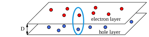
Figure 1: Electron-hole double layer, where individual pairs of electrons and holes form indirect excitons (blue ellipse) for a sufficiently strong interlayer Coulomb interaction. The effective strength of the latter can be tuned by the distance $D$. These excitons can condense into a superfluid.

II Model: Bogoliubov de Gennes Hamiltonian

Our starting point is the quasiparticle Bogoliubov de Gennes (BdG) Hamiltonian that reads

$$H_{\rm BdG}=\pmatrix{H_{\downarrow}&\Delta\cr\Delta^{\dagger}&-H_{\uparrow}^{*}\cr},$$ (1)

where $H_{\uparrow}$ describes hopping of electrons in the top layer and $H_{\downarrow}$ describes hopping of holes in the bottom layer. $\Delta$ is the interlayer pairing order parameter, calculated in terms of the BCS mean-field approach [17]. In the specific case of a chiral double layer the hopping terms $H_{\uparrow,\downarrow}$ carry a band index $\mu=1,2$ for two bands in each layer that is expanded in terms of Pauli matrices $\{\sigma_{\mu}\}_{\mu=1,2,3}$ with the $2\times 2$ unit matrix $\sigma_{0}$. We assume that $H_{\uparrow,\downarrow}$ are real symmetric matrices with $H_{\uparrow}=H_{\downarrow}=h_{1}\sigma_{1}+h_{2}\sigma_{2}$. Then we can introduce the EHDL Hamiltonian

$$H_{\rm EHDL}=\pmatrix{h_{1}\sigma_{1}+h_{2}\sigma_{2}&\Delta\sigma_{3}\cr\Delta^{*}\sigma_{3}&h_{1}\sigma_{1}+h_{2}\sigma_{2}\cr}$$ (2)

$$=\pmatrix{\sigma_{0}&0\cr 0&\sigma_{3}\cr}\pmatrix{h_{1}\sigma_{1}+h_{2}\sigma_{2}&\Delta\sigma_{0}\cr\Delta^{*}\sigma_{0}&-h_{1}\sigma_{1}-h_{2}\sigma_{2}\cr}\pmatrix{\sigma_{0}&0\cr 0&\sigma_{3}\cr}.$$

For translational invariant hopping terms $h_{1,2}$ and a uniform order parameter $\Delta$ the Fourier representation of $H_{\rm EHDL}$ depends on the 2D wave vector ${\bf k}=(k_{x},k_{y})$ and its gapped quasiparticle dispersion reads $E_{\bf k}=\pm\sqrt{h_{1{\bf k}}^{2}+h_{2{\bf k}}^{2}+|\Delta|^{2}}$. The latter agrees with the dispersion of the BdG Hamiltonian with layers of opposite chirality [10]. An example for a chiral system is the honeycomb lattice, which is bipartite and consists of two triangular sublattices. In this case the sublattice index $\mu=1,2$ refers to the two triangular lattices and the real space coordinates ${\bf r}=(x,y)$ refer only to one of the two triangular lattices.

An important feature of $H_{\rm EHDL}$ is the sign change under a particle-hole transformation

$$H_{\rm EHDL}\to TH_{\rm EHDL}T=-H_{\rm EHDL}\ ,\ \ T=\pmatrix{\sigma_{3}&0\cr 0&-\sigma_{3}\cr},$$ (3)

which reflects a chiral symmetry of quasiparticles in the paired EHDL:

$$U_{\alpha}H_{\rm EHDL}U^{\dagger}_{\alpha}\ ,\ \ U_{\alpha}=\exp(\alpha T).$$ (4)

II.1 Evanescent quasiparticle modes at a domain wall

An inhomogeneous order parameter $\Delta$ breaks translational invariance and divides the layers in different regions for different values of $\Delta$. Here we will consider the case in which only the phase of $\Delta$ changes in space while $|\Delta|$ is uniform. As a Josephson junction [1] we choose a domain wall at $x=0$ along the $y$ direction (cf. Fig. 2), where the order parameter changes. It should be kept in mind here that the domain wall is created by a potential inside the layers, and the corresponding change of the order parameter is obtained via the BCS-like equation. In practice, this requires some tedious calculations [18] and we simply focus here on the domain wall in terms of $\Delta(x)$, following the recipe proposed in Ref. [19], that it is sufficient to consider the simple case in which the phase of $\Delta$ jumps at the domain wall [19, 20]. Thus, we assume for the pairing order parameter

$$\Delta(x)=\cases{\Delta_{-}=|\Delta|e^{-i\theta/2}&$x\leq 0$\cr\Delta_{+}=|\Delta|e^{i\theta/2}&$x>0$\cr}.$$ (5)

Such a discontinuous phase change creates evanescent modes inside the gap that exists for a uniform order parameter [21].

Next, we analyze the effect of the domain wall on the low-energy approximation of the BdG Hamiltonian with $h_{1}\sim iv_{F}\hbar\partial_{x}$, $h_{2}\sim v_{F}\hbar k_{y}\sim 0$ and with the Fermi velocity $v_{F}$. We assume periodic boundary conditions in the $y$-direction such that an eigenmode with $k_{y}=0$ exists. Then we get from Eq. (2)

$$H_{\rm EHDL}=\pmatrix{iv_{F}\hbar\partial_{x}\sigma_{1}+v_{F}\hbar k_{y}\sigma_{2}&\Delta(x)\sigma_{3}\cr\Delta^{*}(x)\sigma_{3}&iv_{F}\hbar\partial_{x}\sigma_{1}+v_{F}\hbar k_{y}\sigma_{2}\cr}.$$ (6)

For the eigenmodes we make the ansatz $\Psi(x)=\psi e^{-bx}$, where $\psi$ is a four-componet spinor and $b$ depends on $x$. This gives for $k_{y}=0$ with ${\bar{b}}=v_{F}\hbar b$ the eigenmode equation

$$H_{\rm EHDL}\Psi(x)=\pmatrix{0&-i{\bar{b}}&\Delta&0\cr-i{\bar{b}}&0&0&-\Delta\cr\Delta^{*}&0&0&-i{\bar{b}}\cr 0&-\Delta^{*}&-i{\bar{b}}&0\cr}\Psi(x)=E\Psi(x),$$ (7)

which has the eigenvalue $-\sqrt{|\Delta|^{2}-{\bar{b}}^{2}}$ with the eigenspinors

$$\psi_{1-}=\pmatrix{1\cr 0\cr-\sqrt{|\Delta|^{2}-{\bar{b}}^{2}}/\Delta\cr-i{\bar{b}}/\Delta\cr},\ \ \psi_{2-}=\pmatrix{0\cr 1\cr i{\bar{b}}/\Delta\cr\sqrt{|\Delta|^{2}-{\bar{b}}^{2}}/\Delta\cr}$$ (8)

and the eigenvalue $\sqrt{|\Delta|^{2}-{\bar{b}}^{2}}$ with the eigenspinors

$$\psi_{1+}=\pmatrix{1\cr 0\cr\sqrt{|\Delta|^{2}-{\bar{b}}^{2}}/\Delta\cr-i{\bar{b}}/\Delta\cr},\ \ \psi_{2+}=\pmatrix{0\cr 1\cr i{\bar{b}}/\Delta\cr-\sqrt{|\Delta|^{2}-{\bar{b}}^{2}}/\Delta\cr}.$$

The $x$-dependent step function ${\bar{b}}(x)$ with

$${\bar{b}}(x)=\cases{{\bar{b}}_{-}&$x<0$\cr{\bar{b}}_{+}&$x\geq 0$\cr}$$

must be determined by the matching conditions at the domain wall at $x=0$ as

$$\frac{{\bar{b}}_{+}}{\Delta_{+}}=\frac{{\bar{b}}_{-}}{\Delta_{-}},$$ (9)

where the energies of these modes must be the same: $\sqrt{|\Delta|^{2}-{\bar{b}}_{-}^{2}}=\sqrt{|\Delta|^{2}-{\bar{b}}_{+}^{2}}$. The latter is the case for ${\bar{b}}_{+}^{2}={\bar{b}}_{-}^{2}$. Together with Eq. (5) this implies ${\bar{b}}_{-}={\bar{b}}_{+}e^{-i\theta}$ and ${\bar{b}}_{+}^{2}=|\Delta|^{2}$. This is satisfied for $\theta=\pi$, which implies ${\bar{b}}_{-}=-{\bar{b}}_{+}$, $\Delta_{\pm}=\pm i|\Delta|$ and

$$\frac{{\bar{b}}_{\pm}}{\Delta_{\pm}}=-i\frac{{\bar{b}}_{+}}{|\Delta|}.$$ (10)

Then we get an exponential decay on both sides of the domain wall for ${\bar{b}}_{\pm}=\pm|\Delta|$.

It should be noted that the mean-field equation is $U(1)$ invariant, i.e., the global phase of the order parameter is not fixed. For instance, a global $U(1)$ transformation $\pm i|\Delta|\to\pm|\Delta|$ gives a real pairing order parameter.

The matching conditions lead to two zero-energy modes

$$\Psi_{1}=\frac{1}{{\cal N}}\pmatrix{1\cr 0\cr 0\cr 1\cr}e^{-|\Delta||x|/\hbar v_{F}}\ ,\ \ \Psi_{2}=\frac{1}{{\cal N}}\pmatrix{0\cr 1\cr-1\cr 0\cr}e^{-|\Delta||x|/\hbar v_{F}}$$ (11)

with the normalization ${\cal N}=\sqrt{2v_{F}\hbar/|\Delta|}$. This means that $E=0$ represents an exceptional point [22], where the four-dimensional eigenspace defined in Eq. (8) coalesces to a two-dimensional eigenspace of zero-energy modes. In the context of line defects in the BdG Hamiltonian the appearance of exceptional points has been discussed recently in Ref. [23]. It should be noted that the zero-energy eigenmodes in Eq. (11) are real (i.e., they are Majoranas). Therefore, any superposition of the two zero-energy modes $\Phi=a_{1}\Psi_{1}+a_{2}\Psi_{2}$ with complex coefficients $a_{j}=|a_{j}|e^{i\varphi_{j}}$ (and normalization $|a_{1}|^{2}+|a_{2}|^{2}=1$) is also a zero-energy mode. Consequently, these eigenmodes are complex in general and only real for a special choice of the coefficients. Since both zero-energy eigenmodes in Eq. (11) decay exponentially with $|x|$, we must apply an additional condition to obtain a unique solution for the physical system. Based on the idea that the zero-energy eigenmodes represent a current density near the domain wall, which couples through the Josephson effect to the macroscopic supercurrent [10], we determine a unique solution by fixing the current.

Figure 2: Electron-hole double layer with domain walls (red lines), which is given by a sign jump of the pairing order parameter. The local quasiparticle currents (blue arrows) flow in the same (opposite) direction in the two layers parallel (perpendicular) to the domain walls.

III Current conservation: continuity equations

Due to the absence of interlayer tunneling, the current is conserved in each layer separately. We project the zero-energy mode $\Phi$ to the modes $\Phi_{\uparrow,\downarrow}$ of the individual layers as

$$\Phi=\pmatrix{\Phi_{\uparrow}\cr\Phi_{\downarrow}\cr}\ \ {\rm with}\ \ \Phi_{\uparrow}=\pmatrix{a_{1}\cr a_{2}\cr}\frac{e^{-|\Delta||x|/\hbar v_{F}}}{{\cal N}}\ ,\ \ \Phi_{\downarrow}=\pmatrix{-a_{2}\cr a_{1}\cr}\frac{e^{-|\Delta||x|/\hbar v_{F}}}{{\cal N}}.$$ (12)

Then the BdG equation [24] yields the continuity equations with the quasiparticle current operator $j_{x}=\frac{i}{\hbar}[H_{\rm EHDL},x]$. We obtain for the top layer

$$\partial_{t}\Phi_{\uparrow}\cdot\Phi_{\uparrow}+\partial_{x}j_{x\uparrow}=i\frac{\Delta}{\hbar}\Psi^{*}_{\downarrow}\sigma_{3}\Psi_{\uparrow}-i\frac{\Delta^{*}}{\hbar}\Psi^{*}_{\uparrow}\sigma_{3}\Psi_{\downarrow}=-\frac{i}{v_{F}\hbar^{2}}(\Delta-\Delta^{*})|\Delta|Re(a_{1}a_{2}^{*})e^{-2|\Delta||x|/\hbar v_{F}}$$ (13)

and for the bottom layer

$$\partial_{t}\Phi_{\downarrow}\cdot\Phi_{\downarrow}+\partial_{x}j_{x\downarrow}=i\frac{\Delta^{*}}{\hbar}\Psi^{*}_{\uparrow}\sigma_{3}\Psi_{\downarrow}-i\frac{\Delta}{\hbar}\Psi^{*}_{\downarrow}\sigma_{3}\Psi_{\uparrow}=\frac{i}{v_{F}\hbar^{2}}(\Delta-\Delta^{*})|\Delta|Re(a_{1}a_{2}^{*})e^{-2|\Delta||x|/\hbar v_{F}},$$ (14)

where $i(\Delta-\Delta^{*})=-2sgn(x)|\Delta|$. The expressions on the right-hand sides of the continuity equations define supercurrents $j^{s}_{x\uparrow,\downarrow}$ through the relation

$$\partial_{x}j^{s}_{x\uparrow,\downarrow}=\mp 2sgn(x)\frac{|\Delta|^{2}}{v_{F}\hbar^{2}}Re(a_{1}a_{2}^{*})e^{-2|\Delta||x|/\hbar v_{F}}.$$ (15)

After the $x$–integration from the domain wall to some position $x$ this expression provides the $x$-components of the supercurrents as

$$j^{s}_{x\uparrow,\downarrow}(x)=\mp\frac{|\Delta|}{\hbar}Re(a_{1}a_{2}^{*})(1-e^{-2|\Delta||x|/\hbar v_{F}}),$$ (16)

which vanishes at the domain wall $x=0$. Moreover, the $x$-components of the quasiparticle currents $j_{x\uparrow,\downarrow}$ read

$$j_{x\uparrow}=-j_{x\downarrow}=-v_{F}\Phi_{\uparrow}\cdot\sigma_{1}\Phi_{\uparrow}=-\frac{|\Delta|}{\hbar}Re(a_{1}a_{2}^{*})e^{-2|\Delta||x|/\hbar v_{F}}.$$ (17)

The stationary case $\partial_{t}\Phi_{\uparrow}\cdot\Phi_{\uparrow}=\partial_{t}\Phi_{\downarrow}\cdot\Phi_{\downarrow}=0$ provides the condition

$$\partial_{x}j^{s}_{x\uparrow,\downarrow}+\partial_{x}j_{x\uparrow,\downarrow}=\pm 2sgn(x)\left[-\frac{|\Delta|^{2}}{v_{F}\hbar^{2}}Re(a_{1}a_{2}^{*})e^{-2|\Delta||x|/\hbar v_{F}}+\frac{|\Delta|^{2}}{v_{F}\hbar^{2}}Re(a_{1}a_{2}^{*})e^{-2|\Delta||x|/\hbar v_{F}}\right]=0$$

on both side of the domain wall. Finally, the $y$-components of the quasiparticle currents

$$j_{y\uparrow}=j_{y\downarrow}=-v_{F}\Phi_{\downarrow}\cdot\sigma_{2}\Phi_{\downarrow}=-\frac{|\Delta|}{\hbar}Im(a_{1}a_{2}^{*})e^{-2|\Delta||x|/\hbar v_{F}}$$ (18)

yield the vorticities of the quasiparticle currents

$$(\nabla\times{\bf j}_{\uparrow,\downarrow})_{z}=\partial_{x}j_{y\uparrow,\downarrow}=-2sgn(x)\frac{|\Delta|^{2}}{v_{F}\hbar^{2}}Im(a_{1}a_{2}^{*})e^{-2|\Delta||x|/\hbar v_{F}}.$$ (19)

Thus, the vorticity is the same in both layers but has the opposite sign for the two sides of the domain wall. When the modes in the top and in the bottom layer are orthogonal ($\Phi_{\uparrow}\cdot\Phi_{\downarrow}\propto iIm(a_{1}a_{2}^{*})|\Delta|=0$), the quasiparticle current has no $y$-component and the vorticity vanishes. This is the case for the Majorana modes.

These results reflect that the domain wall creates quasiparticle zero-energy modes, which are associated with local quasiparticle currents and, through the Josephson effect, are connected to the macroscopic supercurrents. To avoid any additional contribution of zero-energy modes we must prevent other edges, such as the geometric boundaries in Fig. 2. This is possible by making the system compact by gluing the double layers at the boundaries. The result of this procedure is presented as a torus with two domain walls in Fig. 3. Such a geometry can be realized as the surface of a ring-shaped topological insulator.

Figure 3: After gluing the double layer in Fig. 2 we form a torus. Then the global current ${\bf I}$ winds along the two domain walls around the torus.

IV Discussion and Conclusion

The results of Sect. III reflect an intimate relationship between the macroscopic supercurrent and the zero-energy eigenmode of the quasiparticles via the Josephson effect. This is characterized by the angle $\alpha$ ($-\alpha$) that exists between the current and the domain wall in the top (bottom) layer. Using the expressions in Eqs. (17) and (18) we obtain for the phases $\varphi_{1}$, $\varphi_{2}$ of the eigenmode coefficients $a_{1}$ and $a_{2}$ the relation

$$\alpha=\arctan(j_{y\uparrow}/j_{x\uparrow})=-\arctan(j_{y\downarrow}/j_{x\downarrow})=\frac{\pi}{2}+\varphi_{2}-\varphi_{1},$$ (20)

such that the relative phase of the eigenmode coefficients are determined by the current direction. This offers a direct access to this mode, provided that an external field couples to the dipole moment of the excitons to control the supercurrent. In particular, a real (Majorana) mode appears for $\alpha=\pi/2$ when the current flows perpendicular to the domain wall.

Our calculation was performed for the special example with a jump of the order parameter phase. Similar calculations can be performed for other shapes of $\Delta(x)=|\Delta|e^{i\alpha(x)}$, provided that the order parameter phase represents a kink with a global phase change $\pi$ from one boundary to the other in $x$ direction. Although the chiral Josephson effect will not be changed qualitatively, the decay of the wavefunctions and of the current densities might be different. In particular, a broader Josephson junction might have different modes (cf. discussion in Ref. [21]).

References

- Josephson [1962] B. Josephson, Possible new effects in superconductive tunnelling, Physics Letters 1, 251 (1962).
- Anderson and Rowell [1963] P. W. Anderson and J. M. Rowell, Probable observation of the josephson superconducting tunneling effect, Phys. Rev. Lett. 10, 230 (1963).
- Tanaka et al. [1999] Y. Tanaka, T. Hirai, K. Kusakabe, and S. Kashiwaya, Theory of the josephson effect in a superconductor/one-dimensional electron gas/superconductor junction, Phys. Rev. B 60, 6308 (1999).
- Asano et al. [2003] Y. Asano, Y. Tanaka, M. Sigrist, and S. Kashiwaya, Josephson current in s-wave-superconductor/ junctions, Phys. Rev. B 67, 184505 (2003).
- Kwon et al. [2004] H.-J. Kwon, K. Sengupta, and V. M. Yakovenko, Fractional ac josephson effect in p- and d-wave superconductors, The European Physical Journal B - Condensed Matter and Complex Systems 37, 349 (2004).
- Pereverzev et al. [1997] S. V. Pereverzev, A. Loshak, S. Backhaus, J. C. Davis, and R. E. Packard, Quantum oscillations between two weakly coupled reservoirs of superfluid 3he, Nature 388, 449 (1997).
- Sukhatme et al. [2001] K. Sukhatme, Y. Mukharsky, T. Chui, and D. Pearson, Observation of the ideal josephson effect in superfluid 4he, Nature 411, 280 (2001).
- Cataliotti et al. [2001] F. S. Cataliotti, S. Burger, C. Fort, P. Maddaloni, F. Minardi, A. Trombettoni, A. Smerzi, and M. Inguscio, Josephson junction arrays with bose-einstein condensates, Science 293, 843 (2001), https://www.science.org/doi/pdf/10.1126/science.1062612 .
- Albiez et al. [2005] M. Albiez, R. Gati, J. Fölling, S. Hunsmann, M. Cristiani, and M. K. Oberthaler, Direct observation of tunneling and nonlinear self-trapping in a single bosonic josephson junction, Phys. Rev. Lett. 95, 010402 (2005).
- Ziegler et al. [2022] K. Ziegler, A. Sinner, and Y. E. Lozovik, Anomalous josephson effect of -wave pairing states in chiral double layers, Phys. Rev. Lett. 128, 157001 (2022).
- Qi and Zhang [2011] X.-L. Qi and S.-C. Zhang, Topological insulators and superconductors, Rev. Mod. Phys. 83, 1057 (2011).
- Burkov [2015] A. A. Burkov, Chiral anomaly and transport in weyl metals, Journal of Physics: Condensed Matter 27, 113201 (2015).
- Sinner et al. [2020] A. Sinner, Y. E. Lozovik, and K. Ziegler, Pairing transition in a double layer with interlayer Coulomb repulsion, Physical Review Research 2, 033085 (2020), arXiv:1912.13257 [cond-mat.supr-con] .
- Lozovik and Yudson [1976] Y. E. Lozovik and V. I. Yudson, A new mechanism for superconductivity: pairing between spatially separated electrons and holes, Soviet Journal of Experimental and Theoretical Physics 44, 389 (1976).
- Lozovik and Poushnov [1997] Y. E. Lozovik and A. V. Poushnov, Magnetism and josephson effect in a coupled quantum well electron-hole system, Physics Letters A 228, 399 (1997).
- Geim and Grigorieva [2013] A. K. Geim and I. V. Grigorieva, Van der waals heterostructures, Nature 499, 419 (2013).
- Bardeen et al. [1957] J. Bardeen, L. N. Cooper, and J. R. Schrieffer, Theory of superconductivity, Phys. Rev. 108, 1175 (1957).
- Spuntarelli et al. [2010] A. Spuntarelli, P. Pieri, and G. Strinati, Solution of the bogoliubov–de gennes equations at zero temperature throughout the bcs–bec crossover: Josephson and related effects, Physics Reports 488, 111 (2010).
- Read and Green [2000] N. Read and D. Green, Paired states of fermions in two dimensions with breaking of parity and time-reversal symmetries and the fractional quantum Hall effect, Phys. Rev. B 61, 10267 (2000).
- Fradkin [2013] E. Fradkin, Field Theories of Condensed Matter Physics, Field Theories of Condensed Matter Physics (Cambridge University Press, 2013).
- Sauls [2018] J. A. Sauls, Andreev bound states and their signatures, Philosophical Transactions of the Royal Society of London Series A 376, 20180140 (2018), 1805.11069 [cond-mat.supr-con] .
- Kato [1976] T. Kato, Perturbation theory for linear operators; 2nd ed., Grundlehren der mathematischen Wissenschaften A Series of Comprehensive Studies in Mathematics (Springer, Berlin, 1976).
- Mandal [2015] I. Mandal, Exceptional points for chiral majorana fermions in arbitrary dimensions, EPL (Europhysics Letters) 110, 67005 (2015).
- Sigal [2022] I. Sigal, Differential equations of quantum mechanics, Quart. Appl. Math. 80, 451 (2022).