Efficient First-order Methods for Convex Optimization with Strongly Convex Function Constraints

Abstract

In this paper, we introduce faster first-order primal-dual algorithms for minimizing a convex function subject to strongly convex function constraints. Before our work, the best complexity bound was $\mathcal{O}(1/{\varepsilon})$, and it remains unclear how to improve this result by leveraging the strong convexity assumption. We address this issue by developing novel techniques to progressively estimate the strong convexity of the Lagrangian function. Our approach yields an improved complexity of $\mathcal{O}(1/\sqrt{\varepsilon})$, matching the complexity lower bound for strongly-convex-concave saddle point optimization. We show the superior performance of our methods in sparsity-inducing constrained optimization, notably Google’s personalized PageRank problem. Furthermore, we show that a restarted version of the proposed methods can effectively identify the sparsity pattern of the optimal solution within a finite number of steps, a result that appears to have independent significance.

1 Introduction

In this paper, we are interested in the following convex function-constrained problem:

$$\begin{split}\mathop{\min}_{\text{$\mathbf{x}$}\in\mathbb{R}^{n}}&\quad f(\text{$\mathbf{x}$})\\ \mathrm{s.t.}&\quad g_{i}(\text{$\mathbf{x}$})\leq 0,\ 1\leq i\leq m,\end{split}$$ (1)

where $f:\mathbb{R}^{n}\to\mathbb{R}$ is a convex continuous function and $g_{i}:\mathbb{R}^{n}\to\mathbb{R}$, $i=1,2,\ldots,m$, are strongly convex continuous functions. An important application of this problem, commonly encountered in statistics and engineering, involves the objective $f(\mathbf{x})$ as a proximal-friendly regularizer and $g_{i}(\mathbf{x})$ as a data-driven loss function used to gauge model fidelity.

To apply first-order methods for the above function-constrained problems, a common strategy involves a double-loop procedure that repeatedly employs fast first-order methods, such as Nesterov’s accelerated method, to solve specific strongly convex proximal subproblems. Popular methods among this category include Augmented Lagrangian methods [19, 33], level-set methods [22], penalty methods [18]. When both $f(\mathbf{x})$ and $g_{i}(\mathbf{x})$ are convex and smooth (or composite), it has been found that these double-loop algorithms can attain an iteration complexity of $\mathcal{O}(1/\varepsilon)$ to achieve an $\varepsilon$-error in both the optimality gap and constraint violation. When the objective is strongly convex, the complexity can be further improved to $\mathcal{O}(1/\sqrt{\varepsilon})$ ([33, 22]).

In contrast to these double-loop algorithms, single-loop algorithms remain popular due to their simplicity in implementation. Along this research line, [32] developed a first-order algorithm based on linearizing the augmented Lagrangian function, which obtains an iteration complexity of $\mathcal{O}(1/\varepsilon)$. [34] extended the augmented Lagrangian method to stochastic function-constrained problems where both objective and constraint exhibit an expectation form. Viewing (1) as a special case of the min-max problem:

$$\min_{\mathbf{x}\in\mathbb{R}^{n}}\max_{\mathbf{y}\in\mathbb{R}^{m}}\ \mathcal{L}(\mathbf{x},\mathbf{y}):=f(\mathbf{x})+\sum_{i=1}^{m}y_{i}{g_{i}(\mathbf{x})},\quad\text{s.t.}\ y_{i}\geq 0,\ i=1,2,\ldots,m,$$ (2)

[11] proposed to solve (1) and (2) by an accelerated primal-dual method (APD), which generalizes the primal-dual hybrid gradient method [5] initially developed for saddle point optimization with bilinear coupling term. Under mild conditions, APD achieves the best iteration complexity of $\mathcal{O}(1/\varepsilon)$ for general convex constrained problem and a further improved complexity of $\mathcal{O}(1/\sqrt{\varepsilon})$ when $f(\mathbf{x})$ is strongly convex. The later work [3] proposed a unified constrained extrapolation method that can be applied to both deterministic and stochastic constrained optimization problems.

Despite these recent progresses, to the best of our knowledge, all available algorithms are suboptimal in the presence of strongly convex function constraints (1). Specifically, direct applications of previously discussed algorithms yield an $\mathcal{O}(1/\varepsilon)$ complexity, which is inferior to the $\mathcal{O}(1/\sqrt{\varepsilon})$ optimal bound for strongly-convex-concave saddle point problem [23]. It is somewhat unsatisfactory that the strong convexity of $g(\mathbf{x})$ has not been found helpful in further algorithmic acceleration. The core underlying issue arises from the dynamics of saddle point optimization: it is the strong convexity of $\mathcal{L}(\cdot,\mathbf{y})$ that offers more potential acceleration advantages, yet the strong convexity of $\mathcal{L}(\cdot,\mathbf{y})$ is substantially harder to estimate than that of $g(\mathbf{x})$. This difficulty is compounded by the interplay between $g(\mathbf{x})$ and the varying dual sequence $\{\mathbf{y}_{k}\}$. This challenge naturally leads us to question: Is it possible to further improve the convergence rate of first-order methods for solving the strongly convex constrained problem (1)?

Key intuitions

We make a mild assumption that at least one of the constraints $\{g_{i}(\mathbf{x})\}$ is active at the optimal solution. Without it, we would essentially be dealing with an unconstrained optimization that does not rely on $g(\mathbf{x})$. Additionally, this assumption ensures strict separation between the origin and the subdifferential at optimal solution $\partial f(\mathbf{x}^{*})$. By leveraging the structures of such an objective function and the strongly convex constraints, we develop new lower bounds for the norm of optimal dual variables $\|\mathbf{y}^{*}\|$. This derived bound, valid under mild assumptions and easily computable using the generated iterates, allows us to effectively harness the strong convexity of the Lagrangian function and apply more aggressive stepsizes. As a result, we are able to develop novel adaptive accelerated methods that achieve sharper convergence rates compared to state-of-the-art algorithms.

Applications in sparsity-constrained optimization

We consider the constrained Lasso-type problem, which minimizes a sparsity-inducing regularizer while explicitly ensuring data-driven error remains controlled:

$$\min_{\mathbf{x}\in\mathbb{R}^{n}}\ \|\mathbf{x}\|_{1}\quad\text{s.t.}\ g(\mathbf{x})\leq 0,$$ (3)

where $g(\cdot)$ is a convex smooth loss term. A motivating application is the approximate personalized PageRank problem [9], where $g(\mathbf{x})=\frac{1}{2}\langle\mathbf{x},Q\mathbf{x}\rangle-\langle\mathbf{b},\mathbf{x}\rangle$ is strongly convex quadratic and $Q$ integrates the graph Laplacian with an identity matrix. Compared to the standard Lasso problem [30]

$$\min_{\mathbf{x}\in\mathbb{R}^{n}}\ g(\mathbf{x})+\lambda\|\mathbf{x}\|_{1},$$ (4)

the constrained problem (3) offers enhanced control over the data fitting error. This advantage, however, is counterbalanced by the challenge of dealing with a nonlinear constraint. Besides concerns about the efficiency in solving (3), it is often desired to show the active set (or sparsity) identification, namely, the nonzero patterns of the optimal solution $\mathbf{x}^{*}$ can be identified by the solution sequence $\{\mathbf{x}_{k}\}$ in a finite number of iterations. Identifying the embedded solution structure within a broader context is referred to as the manifold identification problem [31, 12]. Exploiting the sparsity pattern is particularly desirable in large-scale PageRank problems, as it could result in significant runtime savings. For the regularized Lasso-type problem (4), it has been known that proximal gradient methods (e.g. [14, 20, 25]) possess the finite active-set identification property. Specifically, [25] introduced “active set complexity”, which is defined as the number of iterations required before an algorithm is guaranteed to have reached the optimal manifold, and they proved the proximal gradient method with constant stepsize can identify the optimal manifold in a finite number of iterations. However, for the constrained problem (3), it remains unclear whether first-order methods can identify the sparsity pattern effectively in finite time.

1.1 Contributions

In this paper, we address the aforementioned theoretical questions about strongly convex constrained optimization and the application of sparse optimization. Our contributions are summarized as follows.

First, we present a new accelerated primal-dual algorithm with progressive strong convexity estimation (APDPro) for solving problem (1). APDPro employs a novel strategy to estimate the lower bound of the dual variables, which leads to a gradually refined estimated strong convexity modulus of $\mathcal{L}(\cdot,\mathbf{y})$. With additional cut constraints on the dual update, APDPro is able to separate the dual search space from the origin, which is critical for maintaining the desired strong convexity over the entire solution path. With these two important ingredients, APDPro exhibits an $\mathcal{O}\big{(}{(\|\mathbf{x}_{0}-\mathbf{x}^{*}\|+D_{Y})}/{\sqrt{\varepsilon}}\big{)}$ complexity bound to obtain an $\varepsilon$-error on the function value gap and constraint violation, where $D_{Y}$ is an upper-bound of $\|\mathbf{y}_{0}-\mathbf{y}^{*}\|$. Moreover, we show that for the last iterate to have an $\varepsilon$ error (i.e., $\|\mathbf{x}_{K}-\mathbf{x}^{*}\|^{2}\leq\varepsilon$), APDPro requires a total iteration of $\mathcal{O}\big{(}(\|\mathbf{x}_{0}-\mathbf{x}^{*}\|+\|\mathbf{y}_{0}-\mathbf{y}^{*}\|)/\sqrt{\varepsilon}\big{)}$. Both complexity results appear new in the literature for strongly convex-constrained optimization.

Second, we present a new restart algorithm (rAPDPro) which calls APDPro repeatedly with the input parameters properly changing over time. Different from APDPro, rAPDPro dynamically adjusts the iteration number of APDPro in each epoch based on the progressive strong convexity estimation. We show that rAPDPro exhibits a complexity of $\mathcal{O}\big{(}\log(D_{X}/\sqrt{\varepsilon})+D_{Y}/\sqrt{\varepsilon}\big{)}$ to ensure $\varepsilon$-error in the last iterate convergence where $D_{X}$ is the estimated diameter of the primal feasible domain. While it is difficult to improve the overall $\mathcal{O}(1/\sqrt{\varepsilon})$ bound, rAPDPro appears to be more advantageous when $D_{X}$ and $D_{Y}$ are the same order of $\|\mathbf{x}_{0}-\mathbf{x}^{*}\|$ and $\|\mathbf{y}_{0}-\mathbf{y}^{*}\|$, respectively, and $D_{X}\gg D_{Y}$. In addition, we show that a similar restart strategy can further accelerate the standard APD. The multistage-accelerated primal dual method (msAPD) obtains a comparable $\mathcal{O}(1/\sqrt{\varepsilon})$ complexity of APDPro without introducing additional cut constraint.

Third, we apply our proposed methods to the sparse learning problem (3). In view of the theoretical analysis, all our methods converge at an $\mathcal{O}(1/\sqrt{\varepsilon})$ rate, which is substantially better than the rates of state-of-the-art first-order algorithms. Moreover, we conduct a new analysis to show that the restart algorithm rAPDPro has the favorable feature of identifying the optimal sparsity pattern. Note that such active-set/manifold identification is substantially more challenging to prove due to the coupling of dual variables and constraint functions. To establish the desired property, we develop asymptotic convergence of the dual sequence to the optimal solution, which can be of independent interest.

Comparison with Frank-Wolfe

We note that the strongly convex function constraint in (1) is a special case of a strongly convex set constraint, as demonstrated in [15]. Over the strongly convex set, it has been shown that Frank-Wolfe Algorithm (FW) can obtain convergence rates substantially better than the worst-case $\mathcal{O}(1/\varepsilon)$ rate. Under the bounded gradient assumption, [7, 21] show that FW obtains linear convergence over a strongly convex set. [10] shows that FW obtains an $\mathcal{O}(1/\sqrt{\varepsilon})$ rate when the gradient is the order of the square root of the function value gap. For more recent progress, please refer to [4]. Despite the attractive convergence property, FW exhibits certain limitations when applied to the general function constraints (1) addressed in this paper. Specifically, FW involves a sequence of linear optimization problems throughout the iterations. While linear optimization over certain strongly convex sets, such as $\ell_{p}$-ball, admits a closed-form solution, there exists no efficient routine to handle general function constraints explored in this paper.

1.2 Outline

This paper proceeds as follows. In Section 2, we set notations and make some basic assumptions for the later analysis. Section 3 presents the APDPro algorithm and develops its stepsize rule and complexity rate. Section 4 presents the restart APDPro (rAPDPro) algorithm. Section 5 presents the multistage algorithm msAPD, which does not rely on adding a dual cut constraint. Section 6 applies our proposed method for sparsity-inducing optimization and shows the sparsity identification result for rAPDPro. In Section 7, we conduct numerical results to examine the convergence performance and sparsity identification of our proposed algorithms. Finally, we draw the conclusion in Section 8. All the missing proofs are provided in the appendix sections.

2 Preliminaries

We use bold letters such as $\mathbf{x}$ to represent vectors. Suppose $\mathbf{x}\in\mathbb{R}^{n}$, $q\geq 1$, we use $\|\mathbf{x}\|_{q}=(\sum_{i=1}^{n}|\mathbf{x}_{(i)}|^{q})^{1/q}$ to represent the $l_{q}$-norm, where $\mathbf{x}_{(i)}$ denotes the $i$-th element of $\mathbf{x}$. For brevity, $\|\mathbf{x}\|$ stands for $l_{2}$-norm. For a matrix $A$, we denote the matrix norm induced by 2-norm as $\|A\|=\sup_{\|\mathbf{x}\|\leq 1}\|A\mathbf{x}\|$. We also use $\mathcal{B}(\mathbf{x},r)$ to denote a closed ball centered at $\mathbf{x}$ with radius $r>0$, i.e., $\mathcal{B}(\mathbf{x},r)=\left\{\mathbf{y}\mid\|\mathbf{y}-\mathbf{x}\|\leq r\right\}$. The normal cone of $\mathcal{X}$ at $\mathbf{u}$ is denoted as $\mathcal{N}_{\mathcal{X}}(\mathbf{u}):=\left\{\mathbf{v}\mid\left\langle\mathbf{v},\mathbf{x}-\mathbf{u}\right\rangle\leq 0,\forall\mathbf{x}\in\mathcal{X}\right\}$.

We denote the set of feasible solutions by $\mathcal{X}_{G}:=\left\{\mathbf{x}\mid g_{i}(\mathbf{x})\leq 0,\forall i\in[m]\right\}$ and write the constraint function as $G(\mathbf{x}):=[g_{1}(\mathbf{x}),\ldots,g_{m}(\mathbf{x})]^{\top}$. We assume each $g_{i}(\mathbf{x})$ is a strongly convex function with modulus $\mu_{i}>0$, and denote $\bm{\mu}:=[\mu_{1},\ldots,\mu_{m}]^{\top}$. Let $[m]:=\{1,\ldots,m\}$ for integer $m$. Denote minimum and maximum strongly convexity $\underline{\mu}:=\min_{j\in[m]}\{\mu_{j}\}$, and $\bar{\mu}:=\max_{j\in[m]}\{\mu_{j}\}$. We denote the vector of elements 0 by $\mathbf{0}$.

We state some basic results in nonlinear programming. The Lagrangian function of problem (1) is given by $\mathcal{L}(\mathbf{x},\mathbf{y}):=f(\mathbf{x})+\left\langle\mathbf{y},G(\mathbf{x})\right\rangle$ where $\mathbf{y}\in\mathbb{R}^{m}_{+}$.

Definition 1 (KKT condition).

We say that $\mathbf{x}^{*}$ satisfies the KKT condition of (1) if there exists a Lagrangian multiplier vector $\mathbf{y}^{*}\in\mathbb{R}^{m}_{+}$ such that $\mathbf{0}\in\partial\mathcal{L}(\mathbf{x}^{*},\mathbf{y}^{*})$ and $\mathbf{0}\leq\mathbf{y}^{*}\perp-G(\mathbf{x}^{*})\geq\mathbf{0}$.

The KKT condition is necessary for optimality when a constraint qualification (CQ) holds at $\mathbf{x}^{*}$. Typically, we assume the following Slater’s CQ, which, according to standard convex optimization theory (see [2]), guarantees that an optimal solution is also a KKT point.

Assumption 1 (Slater’s condition).

There exists a strictly feasible point $\widetilde{\mathbf{x}}\in\mathbb{R}^{n}$ such that $G(\widetilde{\mathbf{x}})<\mathbf{0}$.

We require the following assumption to circumvent any trivial solution.

Assumption 2.

The minimizer of function $f(\mathbf{x})$ is infeasible for problem (1), namely, for any $\mathbf{x}_{0}^{*}\in\operatornamewithlimits{argmin}_{\mathbf{x}\in\mathbb{R}^{n}}f(\mathbf{x})$, there exists an $i\in[m]$ such that $g_{i}(\mathbf{x}_{0}^{*})>0$.

Assumption 2 is indeed a mild condition and easily verifiable. Particularly, when $f(\mathbf{x})$ is a sparsity-inducing regularizer, we have the unconstrained minimizer $\mathbf{x}_{0}^{*}=\bm{0}$. Assumption 2 implies that $\mathbf{x}_{0}^{*}$ is infeasible for problem (1). On the other hand, if Assumption 2 fails, we immediately conclude that $\mathbf{x}_{0}^{*}=\bm{0}$ is the optimal solution. Next, we give several useful properties about the optimal solutions of problem (1). The following result on the KKT condition is standard in nonlinear programming. We provide proof for completeness.

Proposition 1.

Suppose Assumption 1 holds. Then, for any optimal solution $\mathbf{x}^{*}$ of problem (1), there exists $\mathbf{y}^{*}\in\mathbb{R}^{m}$ such that the KKT condition holds. Moreover, $\mathbf{y}^{*}$ is bounded within the set $\mathcal{Y}:=\big{\{}\mathbf{y}\in\mathbb{R}_{+}^{m}\mid\|\mathbf{y}\|\leq\bar{c}\big{\}}$, and satisfies $\|\mathbf{y}^{*}\|_{1}\leq\bar{c}$, where $\bar{c}:=\frac{f(\widetilde{\mathbf{x}})-\min_{\mathbf{x}\in\mathbb{R}^{n}}f(\mathbf{x})}{\min_{i\in[m]}\{-g_{i}(\widetilde{\mathbf{x}})\}}$.

Proof.

Under Slater’s CQ, the existence of the KKT condition is a standard result in nonlinear programming. For example, one can refer to [2]. For any $\mathbf{x}\in\mathcal{X}_{G}$, we have

$$f(\mathbf{x})+\left\langle\mathbf{y}^{*},G(\mathbf{x})\right\rangle\geq f(\mathbf{x}^{*})+\left\langle\mathbf{y}^{*},G(\mathbf{x}^{*})\right\rangle=f({\mathbf{x}}^{*}),$$

where the equality is from the complementary slackness. In view of the above result and the Slater’s condition (i.e., $G(\widetilde{\mathbf{x}})<\bm{0}$), we have

$$\begin{split}&f(\widetilde{\mathbf{x}})\geq f(\widetilde{\mathbf{x}})+\left\langle\mathbf{y}^{*},G(\widetilde{\mathbf{x}})\right\rangle\geq f(\mathbf{x}^{*}),\\ \text{$\Rightarrow$}&\|\mathbf{y}^{*}\|_{1}\min_{i\in[m]}\{-g_{i}(\widetilde{\mathbf{x}})\}\leq-\left\langle\mathbf{y}^{*},G(\widetilde{\mathbf{x}})\right\rangle\leq f(\widetilde{\mathbf{x}})-f(\mathbf{x}^{*}),\\ \Rightarrow&\|\mathbf{y}^{*}\|\leq\|\mathbf{y}^{*}\|_{1}\leq\frac{f(\widetilde{\mathbf{x}})-f(\mathbf{x}^{*})}{\min_{i\in[m]}\{-g_{i}(\widetilde{\mathbf{x}})\}}\leq\bar{c},\end{split}$$ (5)

where the last inequality is by $f(\mathbf{x}^{*})\geq\min_{\mathbf{x}\in\mathbb{R}^{n}}f(\mathbf{x})$. ∎

Proposition 2.

Under Assumption 2, problem (1) has a unique optimal solution $\mathbf{x}^{*}$. Let $\mathcal{Y}^{*}:=\operatornamewithlimits{argmax}_{\mathbf{y}\in\mathbb{R}_{+}^{m}}\mathcal{L}(\mathbf{x}^{*},\mathbf{y})$ denote the set containing all the optimal dual variables, then $\mathcal{Y}^{*}$ is a convex set.

Proof.

We prove the uniqueness property by contradiction. Suppose that there exist $(\mathbf{x}^{*},\mathbf{y}^{*})$, $(\widetilde{\mathbf{x}}^{*},\tilde{\mathbf{y}}^{*})$ satisfying the KKT condition, then from the complementary slackness, optimality of $\mathbf{x}^{*}$ and $\tilde{\mathbf{x}}^{*}$, we have

$$\mathcal{L}(\mathbf{x}^{*},\mathbf{y}^{*})=f(\mathbf{x}^{*})=f(\widetilde{\mathbf{x}}^{*})=\mathcal{L}(\widetilde{\mathbf{x}}^{*},\tilde{\mathbf{y}}^{*}).$$

Moreover, we have $\mathcal{L}(\widetilde{\mathbf{x}}^{*},\tilde{\mathbf{y}}^{*})\leq\mathcal{L}(\mathbf{x}^{*},\tilde{\mathbf{y}}^{*})\leq\mathcal{L}(\mathbf{x}^{*},\mathbf{y}^{*}).$ Hence, we must have $\mathcal{L}(\widetilde{\mathbf{x}}^{*},\tilde{\mathbf{y}}^{*})=\mathcal{L}(\mathbf{x}^{*},\tilde{\mathbf{y}}^{*})$. However, since Assumption 2 implies $\tilde{\mathbf{y}}^{*}\neq\bm{0}$, the strongly convex function $\mathcal{L}(\cdot,\tilde{\mathbf{y}}^{*})$ has a unique optimizer. Therefore, we conclude that $\mathbf{x}^{*}=\widetilde{\mathbf{x}}^{*}$.

Next, we show that the set of optimal dual variables for problem (1) is convex. Suppose that there exist two optimal dual variables $\mathbf{y}_{1}^{*}$ and $\mathbf{y}_{2}^{*}$ for the unique primal variable $\mathbf{x}^{*}$, both satisfying the KKT condition, then we have $\left\langle\mathbf{y}_{1}^{*},G(\mathbf{x}^{*})\right\rangle=\left\langle\mathbf{y}_{2}^{*},G(\mathbf{x}^{*})\right\rangle=0$. This implies that any linear combination of $\mathbf{y}_{1}^{*}$ and $\mathbf{y}_{2}^{*}$ satisfy KKT condition, i.e., $\left\langle a\mathbf{y}_{1}^{*}+b\mathbf{y}_{2}^{*},G(\mathbf{x}^{*})\right\rangle=0,\forall a,b$. From Proposition 1, we know any optimal dual variable falls into a bounded convex set $\mathcal{Y}$, which completes the proof. ∎

In view of Assumption 2, Proposition 2, and closeness of the subdifferential set of proper convex functions (Theorem 3.9 [1]), we derive a subdifferential separation result which will be used repeatedly in our algorithm development. Specifically, for the optimal solution $\mathbf{x}^{*}$, we have

$$\mathop{\bf dist}(\partial f(\mathbf{x}^{*}),\mathbf{0})\geq r>0,$$ (6)

for some real value $r$, where $\mathop{\bf dist}(\partial f(\mathbf{x}^{*}),\mathbf{0}):=\min_{\mathbf{\xi}\in\partial f(\mathbf{x}^{*})}\|\xi\|$. We give some important examples for which the lower bound $r$ can be estimated. Suppose $f(\mathbf{x})$ is a Lasso regularizer, i.e., $f(\mathbf{x})=\|\mathbf{x}\|_{1}$, then $r=1$ satisfies (6). More general, consider the group Lasso regularizer, i.e., $f(\mathbf{x})=\sum_{i=1}^{B}p_{i}\|\mathbf{x}_{(i)}\|$, where $\mathbf{x}_{(i)}\in\mathbb{R}^{b_{i}}$ and $\sum_{i=1}^{B}b_{i}=n$, $B$ is the number of blocks, then $r=\min_{i\in[B]}p_{i}$ when $\mathbf{x}^{*}\neq\bm{0}$. Another example is when $f(\mathbf{x})$ is a linear function, namely, $\mathbf{c}^{\top}\mathbf{x}$, where $\mathbf{c}\in\mathbb{R}^{n}$, then we have $r=\|\mathbf{c}\|$.

Condition (6) is similar to the bounded gradient assumption that has been used for accelerating the convergence of the Frank-Wolfe algorithm. Specifically, assuming that $f(\mathbf{x})$ is smooth and its gradient is uniformly bounded by $\|\nabla f(\mathbf{x})\|>c>0$ for any feasible solution $\mathbf{x}$, [7, 21] further improve the convergence rate of Frank-Wolfe algorithm from $\mathcal{O}(1/\varepsilon)$ to $\mathcal{O}\big{(}\log(1/\varepsilon)\big{)}$. Nevertheless, the uniform bounded gradient assumption appears to be stronger than ours, as we only impose the lower boundedness assumption on the optimal solution $\mathbf{x}^{*}$ and allow the objective to be non-differentiable.

Proposition 3.

Under Assumptions 1 and 2, we have

$$\max_{\mathbf{x}_{1},\mathbf{x}_{2}\in\mathcal{X}_{G}}\|\mathbf{x}_{1}-\mathbf{x}_{2}\|\leq\min_{i\in[m]}2\sqrt{\frac{-2g_{i}(\mathbf{x}_{i}^{*})}{\mu_{i}}},$$

where $\mathbf{x}_{i}^{*}=\operatornamewithlimits{argmin}_{\mathbf{x}\in\mathbb{R}^{n}}g_{i}(\mathbf{x})$. Let $\mathcal{X}:=\mathcal{B}\Big{(}\widetilde{\mathbf{x}},\min_{i\in[m]}2\sqrt{\frac{-2g_{i}(\mathbf{x}_{i}^{*})}{\mu_{i}}}+\zeta\Big{)}$, where $\zeta$ is a positive constant, then $\mathbf{x}^{*}\in\mathop{\bf int}\mathcal{X}$.

Proof.

From the strong convexity of $g_{i}(\mathbf{x})$, we have $g_{i}(\mathbf{x})\geq g_{i}(\mathbf{x}_{i}^{*})+\frac{\mu_{i}}{2}\|\mathbf{x}-\mathbf{x}_{i}^{*}\|^{2},$ which implies

$$\|\mathbf{x}-\mathbf{x}_{i}^{*}\|^{2}\leq(g_{i}(\mathbf{x})-g_{i}(\mathbf{x}_{i}^{*}))\frac{2}{\mu_{i}}\leq\frac{-2g_{i}(\mathbf{x}_{i}^{*})}{\mu_{i}},\forall\mathbf{x}\in\mathcal{X}_{G}.$$

In view of the triangle inequality and the above result, for any $\mathbf{x}_{1},\mathbf{x}_{2}\in\mathcal{X}_{G}$, we have

$$\|\mathbf{x}_{1}-\mathbf{x}_{2}\|\leq\|\mathbf{x}_{1}-\mathbf{x}_{i}^{*}\|+\|\mathbf{x}_{2}-\mathbf{x}_{i}^{*}\|\leq 2\sqrt{\frac{-2g_{i}(\mathbf{x}_{i}^{*})}{\mu_{i}}}.$$

Hence, $\mathbf{x}^{*}\in\mathcal{B}\Big{(}\widetilde{\mathbf{x}},\min_{i\in[m]}2\sqrt{\frac{-2g_{i}(\mathbf{x}_{i}^{*})}{\mu_{i}}}\Big{)}$. Since $\zeta$ is a positive constant, we have $\mathbf{x}^{*}\in\textup{int }\mathcal{X}$. ∎

Assumption 3.

There exist $L_{X},L_{G}>0$ such that

$$\|\nabla G(\mathbf{x})-\nabla G(\bar{\mathbf{x}})\| \leq L_{X}\|\mathbf{x}-\bar{\mathbf{x}}\|,\ \ \forall\mathbf{x},\bar{\mathbf{x}}\in\mathcal{X},$$ (7)

$$\|G(\mathbf{x})-G(\bar{\mathbf{x}})\| \leq L_{G}\|\mathbf{x}-\bar{\mathbf{x}}\|,\ \ \forall\mathbf{x},\bar{\mathbf{x}}\in\mathcal{X},$$ (8)

where $\nabla G(\mathbf{x}):=[\nabla g_{1}(\mathbf{x}),\cdots,\nabla g_{m}(\mathbf{x})]\in\mathbb{R}^{n\times m}$.

Proposition 3 and Proposition 1 guarantee that the primal and dual optimal solutions are in an enlarged bounded set $\mathcal{X}$ and $\mathcal{Y}$, respectively, thereby ensuring the Lipschitzness of Lagrangian function in the domain. Combining the inequality (7) and the fact $\|\mathbf{y}\|\leq\|\mathbf{y}\|_{1}\leq\bar{c},\forall\mathbf{y}\in\mathcal{Y}$, we obtain that

$$\|\nabla G(\mathbf{x})\mathbf{y}-\nabla G(\bar{\mathbf{x}})\mathbf{y}\|\leq L_{XY}\|\mathbf{x}-\bar{\mathbf{x}}\|\ \ \forall\mathbf{x},\bar{\mathbf{x}}\in\mathcal{X},\ \forall\mathbf{y}\in\mathcal{Y},$$ (9)

where $L_{XY}=\bar{c}L_{X}$. For set $\mathcal{X}$, $\mathcal{Y}$, we use $D_{X}$ and $D_{Y}$ to denote their diameters, respectively, i.e., $D_{X}:=\max_{\mathbf{x}_{1},\mathbf{x}_{2}\in\mathcal{X}}\|\mathbf{x}_{1}-\mathbf{x}_{2}\|$ and $D_{Y}:=\max_{\mathbf{y}_{1},\mathbf{y}_{2}\in\mathcal{Y}}\|\mathbf{y}_{1}-\mathbf{y}_{2}\|$.

3 APD with progressive strong convexity estimation

In this section, we present the Accelerated Primal-Dual Algorithm with Progressive Strong Convexity Estimation (APDPro) to solve problem (1). In the algorithm running process, we apply a new technique to improve the estimated strong convexity modulus of the Lagrangian function. For problem (1), APDPro achieves the improved convergence rate $\mathcal{O}(1/\sqrt{\varepsilon})$ without relying on the uniform strong convexity assumption [16, 11, 23]. For the rest of this paper, we denote $\mathrm{prox}_{f,\mathcal{X}}(\mathbf{x},\mathbf{z},\eta):=\operatornamewithlimits{argmin}_{\hat{\mathbf{x}}\in\mathcal{X}}f(\hat{\mathbf{x}})+\left\langle\mathbf{z},\hat{\mathbf{x}}\right\rangle+\frac{1}{2\eta}\|\hat{\mathbf{x}}-\mathbf{x}\|^{2}$ as the proximal mapping associated with $f(\cdot)+\langle\mathbf{z},\cdot\rangle$ on $\mathcal{X}$.

We describe the details of APDPro in Algorithm 1. The main component of APDPro contains a dual ascent step to update $\mathbf{y}_{k}$ based on the extrapolated gradient and a primal proximal descent step to update $\mathbf{x}_{k}$. Compared with standard APD [11], APDPro has two more steps. First, line 3 of Algorithm 1 applies a novel cut constraint to separate the dual sequence $\{\mathbf{y}_{k}\}$ from the origin, which allows us to leverage the strong convexity of the Lagrangian function and hence obtain a faster rate of convergence than APD. Second, to use the strong convexity more effectively, in line 9, we perform a progressive estimation of the strong convexity by using the latest iterates $\mathbf{x}_{k}$ and $\bar{\mathbf{x}}_{k}$. Throughout the algorithm process, we use a routine Improve to construct a monotonically increasing sequence $\{\rho_{k}\}$, which provides increasingly refined lower bounds of the strong convexity of the Lagrangian function and better cut constraints for the dual update.

Algorithm 1 Accelerated Primal-Dual Algorithm with Progressive Strong Convexity Estimation (APDPro)

$\tau_{0}>0,\sigma_{0}>0$, $\mathbf{x}_{0}\in\mathcal{X},\mathbf{y}_{0}\in\mathcal{Y},\rho_{0}\geq 0,N>0$

1:Initialize: $\left(\mathbf{x}_{-1},\mathbf{y}_{-1}\right)\leftarrow\left(\mathbf{x}_{0},\mathbf{y}_{0}\right),\bar{\mathbf{x}}_{0}\leftarrow\mathbf{x}_{0}$, $\sigma_{-1}\leftarrow\sigma_{0},\gamma_{0}\leftarrow\sigma_{0}/\tau_{0},T_{0}=0$

2:Set $\Delta_{XY}=\frac{1}{2\tau_{0}}D_{X}^{2}+\frac{1}{2\sigma_{0}}D_{Y}^{2}$ $k=0,1,\ldots,N$

3:$\mathcal{Y}_{k}\leftarrow\left\{\mathbf{y}\in\mathbb{R}_{+}^{m}\mid\|\mathbf{y}\|_{1}\cdot\underline{\mu}\geq\rho_{k}\right\}\bigcap\mathcal{Y}$

4:Compute $\theta_{k}$

5:$\mathbf{z}_{k}\leftarrow(1+\theta_{k})G(\mathbf{x}_{k})-\theta_{k}G(\mathbf{x}_{k-1})$

6:$\mathbf{y}_{k+1}\leftarrow\mathrm{prox}_{\bm{0},\mathcal{Y}_{k}}(\mathbf{y}_{k},-\mathbf{z}_{k},\sigma_{k})$

7:$\mathbf{x}_{k+1}\leftarrow\mathrm{prox}_{f,\mathcal{X}}(\mathbf{x}_{k},\nabla G(\mathbf{x}_{k})\mathbf{y}_{k+1},\tau_{k})$

8:$t_{k}\leftarrow\sigma_{k}/\sigma_{0}$,$\,\,\bar{\mathbf{x}}_{k+1}\leftarrow(T_{k}\bar{\mathbf{x}}_{k}+t_{k}\mathbf{x}_{k+1})/(T_{k}+t_{k})$,$\,\,T_{k+1}\leftarrow T_{k}+t_{k}$

9:Update $\rho_{k+1}\leftarrow$ Improve$\mathbf{x}_{k}$, $\bar{\mathbf{x}}_{k}$, $\frac{\sigma_{0}\tau_{k-1}\Delta_{XY}}{\sigma_{k-1}}$, $\frac{\Delta_{XY}}{T_{k}}$, $\rho_{k}$

10:Update $\gamma_{k+1}$, $\tau_{k+1}$, and $\sigma_{k+1}$ depended on $\rho_{k+1}$

11:Output: $\mathbf{x}_{N+1},\mathbf{y}_{N+1}$ Improve$\mathbf{x}$, $\bar{\mathbf{x}}$, $\beta$, $\bar{\beta}$, $\rho_{\text{old}}$

12: Compute $\rho=\underline{\mu}\cdot\max\bigg{\{}r\big{[}\|\nabla G({\mathbf{x}})\|+L_{X}\sqrt{2\beta}\big{]}^{-1},\Big{[}\frac{L_{X}}{r}\sqrt{\frac{\bar{\beta}}{2\underline{\mu}}}+\sqrt{\frac{L_{X}^{2}\bar{\beta}}{2\underline{\mu}r^{2}}+\frac{\|\nabla G(\bar{\mathbf{x}})\|}{r}}\Big{]}^{-2}\bigg{\}}$

13:Set $\rho_{\text{new}}=\max\{\rho_{\text{old}},\rho\}$

14:$\rho_{\text{new}}$

The Improve step

In order to estimate the strong convexity of the Lagrangian function, we rely on the subdifferential separation (i.e., eq. (6)) to bound the dual variables. From the first-order optimality condition in minimizing $\mathcal{L}(\mathbf{x},\mathbf{y}^{*})$ and the fact that $\mathbf{x}^{*}\in\mathop{\bf int}\mathcal{X}$ (i.e. Proposition 3), we have

$$\bm{0}\in\partial f(\mathbf{x}^{*})+\nabla G(\mathbf{x}^{*})\mathbf{y}^{*}+N_{\mathcal{X}}(\mathbf{x}^{*})=\partial f(\mathbf{x}^{*})+\nabla G(\mathbf{x}^{*})\mathbf{y}^{*}.$$

It follows from (6) that

$$r\leq\|\nabla G(\mathbf{x}^{*})\mathbf{y}^{*}\|\leq\|\nabla G(\mathbf{x}^{*})\|\cdot\|\mathbf{y}^{*}\|\leq\|\mathbf{y}^{*}\|_{1}\|\nabla G(\mathbf{x}^{*})\|,$$ (10)

where the last inequality use the fact that $\|\cdot\|\leq\|\cdot\|_{1}$. Note that the bound $\|\mathbf{y}^{*}\|_{1}\geq{r}/{\|\nabla G(\mathbf{x}^{*})\|}$ can not be readily used in the algorithm implementation because $\mathbf{x}^{*}$ is generally unknown. To resolve this issue, we develop more concrete dual lower bounds by using the generated solution $\hat{\mathbf{x}}$ in the proximity of $\mathbf{x}^{*}$. As we will show in the analysis, APDPro keeps track of two primal sequences $\{\mathbf{x}_{k}\}$ and $\{\bar{\mathbf{x}}_{k}\}$, for which we can establish bounds on $\|\mathbf{x}_{k}-\mathbf{x}^{*}\|^{2}$ and ${(\mathbf{y}^{*})^{\top}\bm{\mu}}\cdot\|\hat{\mathbf{x}}-\mathbf{x}^{*}\|^{2}/2$, respectively. This drives us to develop the following lower bound property.

Proposition 4.

Suppose Assumption 3 holds. Let $\mathbf{y}^{*}\in\mathcal{Y}^{*}$ be a dual optimal solution.

1. Suppose that $\|\hat{\mathbf{x}}-\mathbf{x}^{*}\|^{2}\leq 2\beta$, then we have

   $$\|\mathbf{y}^{*}\|_{1}\geq h_{1}(\hat{\mathbf{x}},\beta):=r\big{[}\|\nabla G(\hat{\mathbf{x}})\|+L_{X}\sqrt{2\beta}\big{]}^{-1}.$$ (11)

2. Suppose $(\mathbf{y}^{*})^{\top}\bm{\mu}\cdot\|\hat{\mathbf{x}}-\mathbf{x}^{*}\|^{2}\leq 2\beta$, then we have

   $$\|\mathbf{y}^{*}\|_{1}\geq h_{2}(\hat{\mathbf{x}},\beta):=\left[\frac{L_{X}}{r}\sqrt{\frac{\beta}{2\underline{\mu}}}+\sqrt{\frac{L_{X}^{2}\beta}{2\underline{\mu}r^{2}}+\frac{\|\nabla G(\hat{\mathbf{x}})\|}{r}}\right]^{-2}.$$ (12)

Proof.

Moreover, using the triangle inequality and (7), we have

$$\|\nabla G(\mathbf{x}^{*})\|-\|\nabla G(\hat{\mathbf{x}})\|\leq\|\nabla G(\mathbf{x}^{*})-\nabla G(\hat{\mathbf{x}})\|\leq L_{X}\|\hat{\mathbf{x}}-\mathbf{x}^{*}\|.$$

Combining the above inequality and (10), we obtain

$$\frac{r}{\|\mathbf{y}^{*}\|_{1}}\leq L_{X}\|\hat{\mathbf{x}}-\mathbf{x}^{*}\|+\|\nabla G(\hat{\mathbf{x}})\|.$$ (13)

Next, we develop more specific lower bounds on $\|\mathbf{y}\|_{1}$. i). Inequality (11) can be easily verified since we have $\|\hat{\mathbf{x}}-\mathbf{x}^{*}\|\leq\sqrt{2\beta}$. ii). Suppose ${(\mathbf{y}^{*})^{\top}\bm{\mu}}\cdot\|\hat{\mathbf{x}}-\mathbf{x}^{*}\|^{2}\leq 2\beta$, then together with (13) we have

$$\frac{r}{\|\mathbf{y}^{*}\|_{1}}\leq L_{X}\sqrt{\frac{2\beta}{(\mathbf{y}^{*})^{\top}\bm{\mu}}}+\|\nabla G(\hat{\mathbf{x}})\|\leq L_{X}\sqrt{\frac{2\beta}{\underline{\mu}\|\mathbf{y}^{*}\|_{1}}}+\|\nabla G(\hat{\mathbf{x}})\|.$$

Note that the above inequality can be expressed as $at^{2}-bt-c\leq 0$ with $t=\|\mathbf{y}^{*}\|_{1}^{-1/2}$, $a=r,b=L_{X}\sqrt{{2\beta}/{\underline{\mu}}}$ and $c=\|\nabla G(\hat{\mathbf{x}})\|$. Standard analysis implies that $t\leq(b+\sqrt{b^{2}+4ac})/{2a}$, which gives the desired bound (12). ∎

Our next goal is to conduct the convergence analysis for APDPro, which can be divided into two parts. First, under the two preconditions (14) and (15), we present the convergence conclusion for the primal-dual gap and optimality gap of problem (1) (see Theorem 1). Next, we derived the convergence rate of APDPro for a specific stepsize selection (see Corollary 1).

Theorem 1.

Suppose that for any $\mathbf{y}^{*}\in\mathcal{Y}^{*}$, we have $(\mathbf{y}^{*})^{\top}\bm{\mu}\geq\rho_{0}$, and there exists a constant $\delta>0$ such that the sequence $\left\{\tau_{k},\sigma_{k},t_{k}\right\}_{k\geq 0}$ satisfies

$$t_{k+1}(\tau_{k+1}^{-1}-\rho_{k+1})\leq t_{k}\tau_{k}^{-1},\quad t_{k+1}\sigma_{k+1}^{-1}\leq t_{k}\sigma_{k}^{-1},\quad t_{k+1}\theta_{k+1}=t_{k},$$ (14)

$$L_{XY}+L_{G}^{2}\sigma_{k}/\delta \leq\tau_{k}^{-1},\quad\theta_{k}\delta/\sigma_{k-1}\leq\sigma_{k}^{-1}.$$ (15)

Then, the set $\mathcal{Y}_{k}$ is nonempty and $\mathcal{Y}^{*}\subseteq\mathcal{Y}_{k}$. Let $\Delta(\mathbf{x},\mathbf{y}):=\frac{1}{2\tau_{0}}\|\mathbf{x}-\mathbf{x}_{0}\|^{2}+\frac{1}{2\sigma_{0}}\|\mathbf{y}-\mathbf{y}_{0}\|^{2}$. The sequence $\{\bar{\mathbf{x}}_{k},\mathbf{x}_{k},\bar{\mathbf{y}}_{k}\}_{k\geq 0}$ generated by APDPro satisfies

$$\frac{t_{K-1}\tau_{K-1}^{-1}}{2T_{K}}\|\mathbf{x}^{*}-\mathbf{x}_{K}\|^{2}+\mathcal{L}(\bar{\mathbf{x}}_{K},\mathbf{y}^{*})-\mathcal{L}(\mathbf{x}^{*},\bar{\mathbf{y}}_{K})\leq\frac{1}{T_{K}}\Delta(\mathbf{x}^{*},\mathbf{y}^{*}),$$ (16)

where $\bar{\mathbf{y}}_{K}=T_{K}^{-1}\sum_{s=0}^{K-1}t_{s}\mathbf{y}_{s}$.

Next, we specify the stepsize selection in Lemma 1 and develop more concrete complexity results in Corollary 1.

Lemma 1.

Let $\hat{\rho}_{k+1}:=\sqrt{\hat{\rho}_{k}^{2}k^{2}+(3\rho_{k+1}\hat{\rho}_{k})k}/({k+1})$, for $k\geq 1$ and $\hat{\rho}_{1}=3\sqrt{{\rho_{1}}/{\tau_{0}}}$. Let $\gamma_{k}$ be an auxiliary sequence with $\gamma_{0}={\sigma_{0}}/{\tau_{0}}$. Suppose $\gamma_{k},\sigma_{k},\tau_{k},\theta_{k},t_{k}$ satisfy:

$$\tau_{0}^{-1}\geq L_{XY}+L_{G}^{2}{\sigma_{0}}/{\delta},\ \textup{where }\delta\in(0,1],$$ (17)

$$\theta_{k}=\frac{\sigma_{k-1}}{\sigma_{k}},\ \gamma_{k+1}=\gamma_{k}\left(1+\rho_{k+1}\tau_{k}\right),\ \tau_{k+1}=\tau_{k}\sqrt{\frac{\gamma_{k}}{\gamma_{k+1}}},$$ (18)

$$t_{k}=\frac{\sigma_{k}}{\sigma_{0}},\ \sigma_{k+1}=\gamma_{k+1}\tau_{k+1}.$$ (19)

Then, we have

$$\gamma_{k}\geq\frac{\hat{\rho}_{k}^{2}\tau_{0}^{2}\gamma_{0}}{9}k^{2}+\gamma_{0},\ \ T_{k}\geq 1+\frac{\tau_{0}}{6}\tilde{\rho}_{k}(k+1)k,\ \ \hat{\rho}_{k}\geq\min\big{\{}\rho_{1},\hat{\rho}_{1}\big{\}},$$ (20)

where $\tilde{\rho}_{k}=2\sum_{s=0}^{k}\hat{\rho}_{s}s/\big{(}k(k+1)\big{)}$ for $k\geq 1$.

Moreover, suppose $\overline{\rho}\tau_{0}\leq 2,$ where $\overline{\rho}=\overline{c}\cdot\overline{\mu},$ then we have

$$\gamma_{k}\leq\gamma_{0}(k+1)^{2}.$$ (21)

Proof.

Note $\tau_{k+1}=\tau_{k}\sqrt{{\gamma_{k}}/{\gamma_{k+1}}}$ implies that $\tau_{k}=\tau_{0}\sqrt{{\gamma_{0}}/{\gamma_{k}}}$. Due to $\gamma_{k+1}=\gamma_{k}(1+\rho_{k+1}\tau_{k})$, we conclude that $\gamma_{k+1}=\gamma_{k}(1+\rho_{k+1}\tau_{k})=\gamma_{k}+\rho_{k+1}\tau_{0}\sqrt{\gamma_{0}\gamma_{k}}$.

Next, we use induction to show that

$$\gamma_{k}\geq\frac{\hat{\rho}_{k}^{2}\tau_{0}^{2}\gamma_{0}}{9}k^{2}+\gamma_{0}.$$ (22)

It is easy to see that the result (22) holds for $k=1$ by the definition of $\hat{\rho}_{1}=3\sqrt{\rho_{1}/\tau_{0}}$ and $\gamma_{1}=(1+\rho_{1}\tau_{0})\gamma_{0}$. Assume (22) holds for all $k=0,\cdots,K$, then we have

$$\begin{split}\gamma_{K+1}&=\gamma_{K}+\rho_{K+1}\tau_{0}\sqrt{\gamma_{0}\gamma_{K}}\\ &\geq\frac{\hat{\rho}_{K}^{2}\tau_{0}^{2}\gamma_{0}}{9}K^{2}+\gamma_{0}+\rho_{K+1}\tau_{0}\sqrt{\gamma_{0}\frac{\hat{\rho}_{K}^{2}\tau_{0}^{2}\gamma_{0}}{9}K^{2}}\\ &\geq\frac{\tau_{0}^{2}\gamma_{0}}{9}(K+1)^{2}\hat{\rho}_{K+1}^{2}+\gamma_{0},\end{split}$$ (23)

which completes our induction. It follows from (22) and the relation among $T_{k}$, $t_{k}$, $\sigma_{k}$, $\tau_{k}$ that, for any $k\geq 1$

$$\begin{split}T_{k}&=\sum_{s=0}^{k}t_{s}\geq 1+\sum_{s=1}^{k}\sqrt{\frac{\tau_{0}}{\sigma_{0}}}\sqrt{\frac{\hat{\rho}_{s}^{2}\tau_{0}^{2}\gamma_{0}}{9}s^{2}+\gamma_{0}}\\ &\geq 1+\sum_{s=1}^{k}\frac{\hat{\rho}_{s}\tau_{0}}{3}s=1+\frac{\tau_{0}}{3}\sum_{s=1}^{k}\hat{\rho}_{s}s=1+\frac{\tau_{0}}{6}\tilde{\rho}_{k}(k+1)k.\end{split}$$ (24)

Similarly, we use induction to prove

$$\hat{\rho}_{k}\geq\min\{\rho_{1},\hat{\rho}_{1}\},\forall k\geq 1.$$ (25)

It is easy to find that $\hat{\rho}_{1}\geq\min\{\rho_{1},\hat{\rho}_{1}\}$. We assume that (25) holds for any $k=1,\ldots,K$. Considering $\hat{\rho}_{K+1}$, we have

$$\begin{split}\hat{\rho}_{K+1}&\geq\frac{1}{K+1}\sqrt{\hat{\rho}_{K}^{2}K^{2}+3\rho_{1}\hat{\rho}_{K}K}\\ &\geq\frac{1}{K+1}\sqrt{\big{(}\min\big{\{}\rho_{1},\hat{\rho}_{1}\big{\}}\big{)}^{2}K^{2}+3\rho_{1}\cdot\min\big{\{}\rho_{1},\hat{\rho}_{1}\big{\}}K}\\ &\geq\min\big{\{}\rho_{1},\hat{\rho}_{1}\big{\}},\end{split}$$

which completes the induction.

In view of (22), (24), and (25), we complete our proof of (20).

Moreover, we use induction to show $\gamma_{k}\leq\gamma_{0}(k+1)^{2}$. It is obvious that the inequality above holds for $k=0$. Assume the inequality holds for all $k=0,\ldots,K$, then we have

$$\begin{split}\gamma_{K+1}&=\gamma_{K}+\rho_{K+1}\tau_{0}\sqrt{\gamma_{0}}\sqrt{\gamma_{K}}\\ &\leq\gamma_{0}(K+1)^{2}+\rho_{K+1}\tau_{0}\gamma_{0}(K+1)\\ &\leq\gamma_{0}\big{[}K^{2}+(2+\overline{\rho}\tau_{0})K+\overline{\rho}\tau_{0}+1\big{]}\\ &\leq\gamma_{0}(K^{2}+4K+4)=\gamma_{0}(K+2)^{2},\end{split}$$

where the second inequality uses the relation $\rho_{k}\leq\overline{\rho},\forall k$, and the last inequality follows from $\overline{\rho}\tau_{0}\leq 2$. ∎

Corollary 1.

Suppose that $\gamma_{k},\sigma_{k},\tau_{k},\theta_{k},t_{k}$ satisfy (17), (18) and (19). Then, for any $K\geq 1$, we have

$$f(\bar{\mathbf{x}}_{K})-f(\mathbf{x}^{*}) \leq\frac{6}{6+\tau_{0}\tilde{\rho}_{K}(K+1)K}\Big{(}\frac{1}{2\tau_{0}}\|\mathbf{x}_{0}-\mathbf{x}^{*}\|^{2}+\frac{D_{Y}^{2}}{2\sigma_{0}}\Big{)},$$ (26)

$$\|[G(\bar{\mathbf{x}}_{K})]_{+}\| \leq\frac{6}{c^{*}(6+\tau_{0}\tilde{\rho}_{K}(K+1)K)}\Big{(}\frac{1}{2\tau_{0}}\|\mathbf{x}_{0}-\mathbf{x}^{*}\|^{2}+\frac{D_{Y}^{2}}{2\sigma_{0}}\Big{)},$$

$$\frac{1}{2}\|\mathbf{x}_{K}-\mathbf{x}^{*}\|^{2} \leq\frac{3\sigma_{0}}{\hat{\rho}_{K}^{2}\tau_{0}^{2}K^{2}+9\gamma_{0}}\Delta(\mathbf{x}^{*},\mathbf{y}^{*}),$$

where $c^{*}:=\big{(}f(\mathbf{x}^{*})-\min_{\mathbf{x}}f(\mathbf{x})\big{)}/{\min_{i\in[m]}\{-g_{i}(\widetilde{\mathbf{x}})\}}>0$.

Remark 1.

In view of Corollary 1, APDPro obtains an iteration complexity of $\mathcal{O}({1}/{\sqrt{\tilde{\rho}_{K}\varepsilon}})$, which is substantially better than the $\mathcal{O}({1}/{\varepsilon})$ bound of APD [11] and ConEx [3] when the strong convexity parameter $\tilde{\rho}_{K}$ is relatively large compared with $\varepsilon$. In addition, we argue that even when $\tilde{\rho}_{K}=O(\varepsilon)$, APDPro can obtain the matching $\mathcal{O}({1}/{\varepsilon})$ bound of the state-of-the-art algorithms. Specifically, using the definition of $\gamma_{k},\sigma_{k}$, we can easily derive the monotonicity of $\{\sigma_{k}\}$. It follows from

$$\sigma_{k+1}=\gamma_{k+1}\tau_{k+1}=\tau_{k}\sqrt{{\gamma_{k}}{\gamma_{k+1}}}=\tau_{k}\gamma_{k}\sqrt{1+\rho_{k+1}\tau_{k}}\geq\gamma_{k}\tau_{k}=\sigma_{k},$$

that $T_{k}=\sum_{s=0}^{k-1}t_{k}=\sigma_{0}^{-1}\sum_{s=0}^{k-1}\sigma_{k}\geq k$. Using a similar argument to that of Corollary 1, we immediately obtain the bound $f(\bar{\mathbf{x}}_{K})-f(\mathbf{x}^{*})\leq\mathcal{O}({1}/{K})$ and $\|[G(\bar{\mathbf{x}}_{K})]_{+}\|\leq\mathcal{O}({1}/{K})$.

Remark 2.

The implementation of APDPro requires knowing an upper bound on $\|\mathbf{y}^{*}\|$. When the bound is unavailable, [11] developed an adaptive APD which still ensures the boundedness of dual sequence via line search. Since our main goal of this paper is to exploit the lower-bound rather than the upper bound of $\|\mathbf{y}^{*}\|$, we leave the extension of our technique to such adaptive APD to the future work.

4 APDPro with a restart scheme

Note that in the worst case, APDPro exhibits an iteration complexity of $\mathcal{O}\big{(}(D_{X}+D_{Y})/\sqrt{\varepsilon}\big{)}$, which has a linear dependence on the diameter. While the $\mathcal{O}({1}/{\sqrt{\varepsilon}})$ is optimal [26], it is possible to improve the complexity with respect to the primal part from $\mathcal{O}\big{(}{D_{X}}/{\sqrt{\varepsilon}}\big{)}$ to $\mathcal{O}\big{(}\log\big{(}{D_{X}}/{\sqrt{\varepsilon}}\big{)}\big{)}$. To achieve this goal, we propose a restart scheme (rAPDPro) that calls APDPro repeatedly and present the details in Algorithm 2. The total iteration number of APDPro in each epoch is an important parameter of the restart algorithm. Inspired by [17], we set the iteration number as a function of the estimated strong convexity, detailed in the TerminateIter procedure. For convenience in describing a double-loop algorithm, we use superscripts for the number of epochs and subscripts for the number of sub-iterations in parameters $\mathbf{x},\mathbf{y},\tau,\text{$\sigma$},\gamma$, e.g., $\mathbf{x}_{1}^{S}$ meaning the $\mathbf{x}$ output of first iterations at $S$-th epoch. To avoid redundancy in the Algorithm 2, we call the APDPro iteration (i.e., line 3-10 of APDPro) directly. Note that the notation system here is identical to that of APDPro, with the only difference being the use of superscripts to distinguish the number of epochs.

Algorithm 2 Restarted APDPro (rAPDPro)

$\rho^{-1}_{N_{-1}}\geq 0,\bar{\sigma}>0$, $\delta\in(0,1]$, $\nu_{0}\in(0,1)$, $\mathbf{x}^{-1}_{N_{-1}},\mathbf{y}^{-1}_{N_{-1}},S$

1:Compute $\bar{\tau}=(1-\nu_{0})\big{(}L_{XY}+\frac{L_{G}^{2}}{\delta}\bar{\sigma}\big{)}^{-1},\bar{\gamma}\leftarrow\bar{\sigma}/\bar{\tau}$ $s=0,1,\ldots,S$

2:Set $\tau_{0}^{s}=\bar{\tau},\sigma_{0}^{s}=\bar{\sigma},(\mathbf{x}_{-1}^{s},\mathbf{y}_{-1}^{s})\leftarrow(\mathbf{x}_{N_{s-1}}^{s-1},\mathbf{y}_{N_{s-1}}^{s-1}),(\mathbf{x}_{0}^{s},\mathbf{y}_{0}^{s})\leftarrow(\mathbf{x}_{N_{s-1}}^{s-1},\mathbf{y}_{N_{s-1}}^{s-1}),\rho_{0}^{s}=\rho_{N_{s-1}}^{s-1}$

3:Set $\Delta_{XY}=\frac{1}{\tau_{0}^{s}}D_{X}^{2}+\frac{1}{2\sigma_{0}^{s}}D_{Y}^{2},\sigma_{-1}^{s}\leftarrow\sigma_{0}^{s},\gamma_{0}^{s}\leftarrow\bar{\gamma},T_{0}^{s}=0,k=0,\hat{\rho}_{0}^{s}=1,N_{s}=\infty$ $k<N_{s}$

4:Run line 3-10 of APDPro with index set $(s,k)$

5:Update $N_{s},\hat{\rho}_{k+1}^{s}\leftarrow$TerminateIter$\hat{\rho}_{k}^{s},\rho_{k+1}^{s},s,k$

6:$k\leftarrow k+1$

7:Output:$\mathbf{x}^{S}_{N_{S}},\mathbf{y}^{S}_{N_{S}}$ TerminateIter$\hat{\rho}_{\text{old}},\rho,s,k$

8: Compute $\hat{\rho}_{\text{new}}=\begin{cases}\frac{1}{k+1}\sqrt{\hat{\rho}_{\text{old}}^{2}k^{2}+3\rho\hat{\rho}_{\text{old}}k}&k>1\\ 3\sqrt{{\rho}/{\tau_{0}}}&k=1\end{cases}$

9:Compute $N=\lceil\max\{6(\hat{\rho}_{\text{new}}\tau_{0}^{s})^{-1},\sqrt{2}^{s}\cdot 3\sqrt{2}D_{Y}/\big{(}\hat{\rho}_{\text{new}}D_{X}\sqrt{\tau_{0}^{s}\sigma_{0}^{s}}\big{)}\}\rceil$

10:$N,\hat{\rho}_{\text{new}}$

In Theorem 2, we show the overall convergence complexity of rAPDPro.

Theorem 2.

Let $\{\mathbf{x}_{0}^{s}\}_{s\geq 0}$ be the sequence generated by rAPDPro, then we have

$$\|\mathbf{x}_{0}^{s}-\mathbf{x}^{*}\|^{2}\leq\Delta_{s}\equiv D_{X}^{2}\cdot 2^{-s},\ \ \ \forall s\geq 0.$$ (27)

As a consequence, rAPDPro will find a solution $\mathbf{x}_{0}^{S}$ such that $\|\mathbf{x}_{0}^{S}-\mathbf{x}^{*}\|^{2}\leq\varepsilon$ for any $\varepsilon\in(0,D_{X}^{2})$ in at most $S:=\big{\lceil}\log_{2}(D_{X}^{2}/\varepsilon)\big{\rceil}$ epochs. Moreover, the overall number of iterations performed by rAPDPro to find such a solution is bounded by

$$T_{\varepsilon}:=\Big{(}\frac{12}{\tilde{\rho}_{1}\tau_{0}^{s}}+2\Big{)}\left\lceil\log_{2}\frac{D_{X}}{\sqrt{\varepsilon}}+1\right\rceil+\Big{(}\frac{6(\sqrt{2}+2)}{\tilde{\rho}_{2}\sqrt{\tau_{0}^{s}\sigma_{0}^{s}}}\Big{)}\cdot\Big{(}\frac{D_{Y}}{\sqrt{\varepsilon}}\Big{)},$$ (28)

where $\sum_{s=0}^{S}(\hat{\rho}_{N_{s}}^{s})^{-1}=(\widetilde{\rho}_{1})^{-1}(S+1)$ and $\sum_{s=0}^{S}{\sqrt{2}^{s}}/{\hat{\rho}_{N_{s}}^{s}}=(\widetilde{\rho}_{2})^{-1}\sum_{s=0}^{S}\sqrt{2}^{s}$.

Proof.

First, we show that the choice of $\tau_{0}^{s}=\bar{\tau},\sigma_{0}^{s}=\bar{\sigma},\forall s\geq 0$ satisfy the condition (17) in Corollary 1: $(\tau_{0}^{s})^{-1}\geq(1-\nu_{0})(\tau_{0}^{s})^{-1}=L_{XY}+c{L_{G}^{2}}\sigma_{0}^{s}/{\delta}$.

Next, we show (27) holds by induction. Clearly, (27) holds for $s=0$. Assume $\|\mathbf{x}_{0}^{s}-\mathbf{x}^{*}\|^{2}\leq\Delta_{s}$ holds for $s=0,\ldots,S-1$. Then by Theorem 1, we have

$$\|\mathbf{x}_{0}^{S}-\mathbf{x}^{*}\|^{2}\leq\frac{\sigma_{0}^{S}\tau_{N_{S}}^{S}}{\sigma_{N_{S}}^{S}}\Big{(}\frac{2}{\tau_{0}^{S}}\Delta_{S}+\frac{1}{\sigma_{0}^{S}}D_{Y}^{2}\Big{)}.$$ (29)

In view of the bound in (20) and the relation between $\tau^{s}_{N_{s}},\sigma^{s}_{N_{s}}$, we can get

$$\frac{\tau_{N_{s}}^{s}}{\sigma_{N_{s}}^{s}}=\frac{1}{\gamma_{N_{s}}^{s}}\leq\frac{9}{\gamma_{0}(\hat{\rho}_{N_{s}}\tau_{0}^{s}N_{s})^{2}}=\frac{9}{\sigma_{0}^{s}\tau_{0}^{s}(\hat{\rho}_{N_{s}}N_{s})^{2}}.$$ (30)

Combining (29) and (30) yields

$$\|\mathbf{x}_{0}^{S}-\mathbf{x}^{*}\|^{2}\leq\frac{18}{(\hat{\rho}_{N_{s}}\tau_{0}^{s}N_{s})^{2}}+\frac{9D_{Y}^{2}}{\sigma_{0}^{s}\tau_{0}^{s}(\hat{\rho}_{N_{s}}N_{s})^{2}}.$$

Since the algorithm sets $N_{s}=\lceil\max\{6(\hat{\rho}_{N_{s}}\tau_{0}^{s})^{-1},\sqrt{2}^{s}\cdot 3\sqrt{2}D_{Y}/\big{(}\hat{\rho}_{N_{s}}D_{X}\sqrt{\tau_{0}^{s}\sigma_{0}^{s}}\big{)}\}\rceil$, it follows that

$$\begin{split}\frac{18}{(\hat{\rho}_{N_{s}}\tau_{0}^{s}N_{s})^{2}}&\leq\frac{18}{(\hat{\rho}_{N_{s}}\tau_{0}^{s})^{2}}\cdot\frac{(\hat{\rho}_{N_{s}}\tau_{0}^{s})^{2}}{36}=\frac{1}{2},\\ \frac{9D_{Y}^{2}}{\sigma_{0}^{s}\tau_{0}^{s}(\hat{\rho}_{N_{s}}N_{s})^{2}}&\leq\frac{9D_{Y}^{2}}{\sigma_{0}^{s}\tau_{0}^{s}\hat{\rho}_{N_{s}}^{2}}\cdot\frac{\hat{\rho}_{N_{s}}^{2}\sigma_{0}^{s}\tau_{0}^{s}D_{X}^{2}}{18D_{Y}^{2}2^{s}}=\frac{1}{2}\cdot 2^{-s}D_{X}^{2}=\frac{1}{2}\Delta_{S},\end{split}$$

which implies the desired result (27).

Let the algorithm run for $S=\big{\lceil}\log_{2}(D_{X}^{2}/{\varepsilon})\big{\rceil}$ epochs, then $\|\mathbf{x}_{0}^{S}-\mathbf{x}^{*}\|^{2}\leq D_{X}^{2}\cdot 2^{-S}\leq\varepsilon$. The total iteration number required by Algorithm 2 for attaining a solution $\mathbf{x}_{0}^{S}$ such that $\|\mathbf{x}_{0}^{S}-\mathbf{x}^{*}\|^{2}\leq\varepsilon$ is

$$\begin{split}\sum_{s=0}^{S}N_{s}\leq&\sum_{s=0}^{S}\Big{\{}\frac{6}{\hat{\rho}^{s}_{N_{s}}\tau_{0}^{s}}+\frac{3\sqrt{2}D_{Y}}{\hat{\rho}^{s}_{N_{s}}D_{X}\sqrt{\tau_{0}^{s}\sigma_{0}^{s}}}\sqrt{2}^{s}+1\Big{\}}\\ \overset{(a)}{=}&\Big{(}\frac{6}{\tilde{\rho}_{1}\tau_{0}^{s}}+1\Big{)}(S+1)+{\frac{3\sqrt{2}D_{Y}}{\tilde{\rho}_{2}D_{X}\sqrt{\tau_{0}^{s}\sigma_{0}^{s}}}}\sum_{s=0}^{S}\sqrt{2}^{s}\\ \leq&\Big{(}\frac{12}{\tilde{\rho}_{1}\tau_{0}^{s}}+2\Big{)}\left\lceil\log_{2}\frac{D_{X}}{\sqrt{\varepsilon}}+1\right\rceil+{\frac{3\sqrt{2}D_{Y}}{\tilde{\rho}_{2}D_{X}\sqrt{\tau_{0}^{s}\sigma_{0}^{s}}}}\cdot\frac{\sqrt{2}^{S+1}-1}{\sqrt{2}-1}\\ \leq&\Big{(}\frac{12}{\tilde{\rho}_{1}\tau_{0}^{s}}+2\Big{)}\left\lceil\log_{2}\frac{D_{X}}{\sqrt{\varepsilon}}+1\right\rceil+{\frac{3\sqrt{2}D_{Y}(\sqrt{2}+1)}{\tilde{\rho}_{2}D_{X}\sqrt{\tau_{0}^{s}\sigma_{0}^{s}}}}\cdot\big{(}\sqrt{2}^{\log_{2}(D_{X}^{2}/\varepsilon)+2}-1\big{)}\\ \leq&\Big{(}\frac{12}{\tilde{\rho}_{1}\tau_{0}^{s}}+2\Big{)}\left\lceil\log_{2}\frac{D_{X}}{\sqrt{\varepsilon}}+1\right\rceil+{\frac{6D_{Y}(\sqrt{2}+2)}{\tilde{\rho}_{2}\sqrt{\tau_{0}^{s}\sigma_{0}^{s}}}}\cdot{\frac{1}{\sqrt{\varepsilon}}},\end{split}$$

where $(a)$ follows from $\sum_{s=0}^{S}(\hat{\rho}_{N_{s}}^{s})^{-1}=(\tilde{\rho}_{1})^{-1}(S+1)$ and $\sum_{s=0}^{S}{\sqrt{2}^{s}}/{\hat{\rho}_{N_{s}}^{s}}=(\tilde{\rho}_{2})^{-1}\sum_{s=0}^{S}\sqrt{2}^{s}$. ∎

Remark 3.

The bound $T_{\varepsilon}$ depends on $\varepsilon$, $\widetilde{\rho}_{1}$ and $\widetilde{\rho}_{2}$. If $\widetilde{\rho}_{1}=O\big{(}(-\log_{2}\sqrt{\varepsilon})^{-1}\big{)}$ or $\widetilde{\rho}_{2}=O(\sqrt{\varepsilon})$, then we have $T_{\varepsilon}=\infty$, which implies that we can not guarantee $\|\mathbf{x}_{0}^{s}-\mathbf{x}^{*}\|\leq\varepsilon$ at finite iterations. $T_{\varepsilon}=\infty$ implies that there exists an epoch with infinite sub-iterations. Hence, rAPDPro is reduced to APDPro if we only consider that epoch.

Remark 4.

Comparison of rAPDPro and APDPro involves a number of factors. In particular, rAPDPro compares favorably against APDPro if $\|\mathbf{x}_{0}-\mathbf{x}^{*}\|=\widetilde{\Omega}(\sqrt{\varepsilon}\log D_{X})$, which is reasonable. Moreover, it should be noted that the complexity bound (28) can be slightly improved if $D_{X}$ is replaced by any tighter upper bound of $\|\mathbf{x}^{s}_{0}-\mathbf{x}^{*}\|$. However, it is still unknown whether we can directly replace $D_{X}$ with $\|\mathbf{x}^{s}_{0}-\mathbf{x}^{*}\|$ in (28).

Dual Convergence

For dual variables, we establish asymptotic convergence to the optimal solution, a key condition for developing the active-set identification scheme in the later section. For the ease in notation, it is more convenient to labeling the generated solution as a whole sequence using a single subscript index: $\mathbf{x}_{1},\mathbf{x}_{2},\ldots,\mathbf{x}_{N};\mathbf{y}_{1},\mathbf{y}_{2},\ldots,\mathbf{y}_{N}$. Hence, we use the index system $j$ and $(s,k)$ interchangeably. Note that $\{\mathbf{x}_{0}^{s+1},\mathbf{y}_{0}^{s+1}\}$ and $\{\mathbf{x}_{N_{s}+1}^{s},\mathbf{y}_{N_{s}+1}^{s}\}$ correspond to the same pair of points. Let

$$\begin{split}Q_{j}(\mathbf{x},\mathbf{y})&:=\frac{(\tau_{j})^{-1}-\rho_{j}}{2}\|\mathbf{x}-\mathbf{x}_{j}\|^{2}+\frac{1}{2\sigma_{j}}\|\mathbf{y}-\mathbf{y}_{j}\|^{2}+\theta_{j}\left\langle\mathbf{y}_{j}-\mathbf{y},G(\mathbf{x}_{j})-G(\mathbf{x}_{j-1})\right\rangle\\ &\ \ +\frac{\theta_{j}}{2\delta/\sigma_{j-1}}\|G(\mathbf{x}_{j})-G(\mathbf{x}_{j-1})\|^{2},\end{split}$$

then we establish an important recursive property about the solution sequence in the following lemma.

Lemma 2.

Assume $\bar{\tau}^{-1}>\overline{\rho}$ and choose $\nu_{0}>0$ such that

$$1>\inf_{j\geq 0}\{\theta_{j}\}\geq\delta+\nu_{0}.$$ (31)

Then there exists an $\nu_{1}>0$ such that for any $j\geq 0$ and any KKT point $(\mathbf{x}^{*},\tilde{\mathbf{y}}^{*})$:

$$0 \leq t_{j}Q_{j}(\mathbf{x}^{*},\tilde{\mathbf{y}}^{*})-t_{j+1}Q_{j+1}(\mathbf{x}^{*},\tilde{\mathbf{y}}^{*})$$

$$\quad-\nu_{1}t_{j}\left[\frac{1}{2\tau_{j}}\|\mathbf{x}_{j+1}-\mathbf{x}_{j}\|^{2}+\frac{1}{2\sigma_{j}}\|\mathbf{y}_{j+1}-\mathbf{y}_{j}\|^{2}\right],$$

$$0 <t_{j}Q_{j}(\mathbf{x}^{*},\tilde{\mathbf{y}}^{*}).$$

Remark 5.

Assumption $(\bar{\tau})^{-1}>\overline{\rho}$ is mild. Since we always choose $\bar{\sigma}$ large enough in rAPDPro, $\bar{\tau}$ can be sufficiently small. Furthermore, since ${\sigma_{k}^{s}}/{\sigma_{k-1}^{s}}=(\theta_{k}^{s})^{-1}=\sqrt{1+\rho_{k}^{s}\tau_{k}^{s}}$, $\{\rho_{k}^{s}\}$ is a bounded sequence due to the boundedness of the dual variable, $\{\tau_{k}^{s}\}$ is monotonically decreasing, then $\inf_{0\leq k\leq N_{s}}\theta_{k}^{s}\geq(1+\overline{\rho}\bar{\tau})^{-1/2}$. Hence, inequality (31) is always satisfiable if we choose proper $\delta,\nu_{0}$ such that $(1+\overline{\rho}\bar{\tau})^{-1/2}\geq\delta+\nu_{0}$.

Theorem 3.

Under all the assumptions of Lemma 2, we have $(\mathbf{x}^{*},\mathbf{y}^{*})$ satisfy the KKT condition, where $\mathbf{y}^{*}$ is any limit point of $\{\mathbf{y}_{j}\}$ generated by rAPDPro.

5 A multi-stage accelerated primal-dual algorithm

Both the previous algorithms need to solve a complicated dual problem that involves a linear cut constraint, posing a potential issue: the associated sub-problem might lack a closed-form solution. To resolve this issue, we propose a new method to obtain the same $\mathcal{O}(1/\sqrt{\varepsilon})$ complexity without introducing a new cut constraint. We present the Multi-Stage Accelerated Primal-Dual Algorithm (msAPD) in Algorithm 3. Motivated by the restart algorithm, our new method is a double-loop procedure for which an accelerated primal-dual algorithm with a pending sub-iteration number (APDPi) is running in each stage. While both APDPi and APDPro employ the Improve step to estimate the dual lower bound, APDPi only relies on the lower bound estimation to change the inner-loop iteration number adaptively, but not the stepsize selection. As a consequence, APDPi does not explicitly add dual cut constraints to warrant strong convexity of the Lagrangian function.

Algorithm 3 Multi-Stage APD (msAPD)

$\bar{\mathbf{x}}^{0}\in\mathcal{X},\bar{\mathbf{y}}^{0}\in\mathcal{Y},\delta\in(0,1],\widetilde{\sigma},S$

1:Initialize: $\rho_{0}^{0}=0$ $s=0,\ldots,S$

2:Compute $\tau_{0}^{s}=\big{(}L_{XY}+\frac{L_{G}^{2}\widetilde{\sigma}}{\delta}\cdot 2^{\frac{s}{2}}\big{)}^{-1},\sigma_{0}^{s}=\widetilde{\sigma}\cdot 2^{\frac{s}{2}}$

3:$(\bar{\mathbf{x}}^{s+1},\bar{\mathbf{y}}^{s+1},\rho^{s+1}_{0})\leftarrow$ APDPi$\tau^{s}_{0},\sigma^{s}_{0},\bar{\mathbf{x}}^{s},\bar{\mathbf{y}}^{s},\rho_{0}^{s},s$

4:Output: $\bar{\mathbf{x}}^{S+1},\bar{\mathbf{y}}^{S+1}$ APDPi$\tau_{0}^{s},\sigma_{0}^{s},\mathbf{x}_{0},\mathbf{y}_{0},\rho_{0}^{s},s$

5:Initialize: $\left(\mathbf{x}_{-1},\mathbf{y}_{-1}\right)\leftarrow\left(\mathbf{x}_{0},\mathbf{y}_{0}\right),\bar{\mathbf{x}}_{0}=\mathbf{x}_{0},k=0,N_{s}=\infty$, $\Delta_{XY}=\frac{1}{2\tau_{0}^{s}}D_{X}^{2}+\frac{1}{2\sigma_{0}^{s}}D_{Y}^{2}$ $k<N_{s}$

6:$\mathbf{z}_{k}\leftarrow 2G(\mathbf{x}_{k})-G(\mathbf{x}_{k-1})$

7:$\mathbf{y}_{k+1}\leftarrow\mathrm{prox}_{\bm{0},\mathcal{Y}}(\mathbf{y}_{k},-\mathbf{z}_{k},\sigma_{0}^{s})$

8:$\mathbf{x}_{k+1}\leftarrow\mathrm{prox}_{f,\mathcal{X}}(\mathbf{x}_{k},\nabla G(\mathbf{x}_{k})\mathbf{y}_{k+1},\tau_{0}^{s})$

9: $\bar{\mathbf{x}}_{k+1}\leftarrow(k\bar{\mathbf{x}}_{k}+\mathbf{x}_{k+1})/(k+1),$

10:$\rho_{k+1}^{s}\leftarrow$Improve$\mathbf{x}_{k},\bar{\mathbf{x}}_{k},\frac{1}{2}D_{X}^{2},\frac{\Delta_{XY}}{k},\rho_{k}^{s}$

11:Compute $N_{s}=\lceil\max\big{\{}\frac{4}{\rho_{k+1}^{s}\tau_{0}^{s}},\frac{D_{Y}^{2}}{\rho_{k+1}^{s}\sigma_{0}^{s}D_{X}^{2}}\cdot 2^{s+1}\big{\}}\rceil$

12:$k\leftarrow k+1$

13:$\bar{\mathbf{x}}_{N_{s}},\bar{\mathbf{y}}_{N_{s}},\rho_{k}^{s}$

We develop the convergence property of the procedure APDPi, which paves the path to proving our main theorem. For the convergence analysis, it suffices to verify that the initial stepsize parameter $\tau^{s}_{0},\sigma^{s}_{0}$ satisfy assumptions in Theorem 4. For completeness, We leave the proof in Section D.

Theorem 4.

Let the sequence $\left\{\bar{\mathbf{x}}_{k}^{s},\bar{\mathbf{y}}_{k}^{s}\right\}_{k\geq 0}$ be generated by APDPi, then for any KKT point $(\mathbf{x}^{*},\mathbf{y}^{*})$ we have

$$\mathcal{L}(\bar{\mathbf{x}}_{K}^{s},\mathbf{y}^{*})-\mathcal{L}(\mathbf{x}^{*},\bar{\mathbf{y}}_{K}^{s}) \leq\frac{1}{K}\Delta^{s}(\mathbf{x}^{*},\mathbf{y}^{*}),$$ (32)

$$\frac{1}{2}\|\bar{\mathbf{x}}_{K}^{s}-\mathbf{x}^{*}\|^{2} \leq\frac{1}{(\mathbf{y}^{*})^{\top}\bm{\mu}K}\Delta^{s}(\mathbf{x}^{*},\mathbf{y}^{*}),$$ (33)

where $\Delta^{s}(\mathbf{x}^{*},\mathbf{y}^{*})\triangleq\frac{1}{2\tau_{0}^{s}}\|\mathbf{x}_{0}^{s}-\mathbf{x}^{*}\|^{2}+\frac{1}{2\sigma_{0}^{s}}\|\mathbf{y}_{0}^{s}-\mathbf{y}^{*}\|^{2}$.

We show that msAPD obtains an $\mathcal{O}(1/\sqrt{\varepsilon})$ rate of convergence to the optimal solution, which matches the complexity of APDPro.

Theorem 5.

Let $\{\bar{\mathbf{x}}_{0}^{s}\}$ be the sequence computed by msAPD. Then, we have

$$\|\bar{\mathbf{x}}_{0}^{s}-\mathbf{x}^{*}\|^{2}\leq\Delta_{s}\equiv D_{X}^{2}\cdot 2^{-s},\quad\forall s\geq 0.$$ (34)

For any $\varepsilon\in(0,D_{X}^{2})$, msAPD will find a solution $\bar{\mathbf{x}}_{0}^{s}\in\mathcal{X}$ such that $\|\bar{\mathbf{x}}_{0}^{s}-\mathbf{x}^{*}\|^{2}\leq\varepsilon$ in at most $\left\lceil\log_{2}{D_{X}^{2}}/{\varepsilon}\right\rceil$ epochs. Moreover, the overall iteration number performed by msAPD to find such a solution is bounded by

$$T_{\varepsilon}=\left(\frac{8L_{XY}}{\rho_{N_{0}}^{0}}+2\right)\left\lceil\log_{2}\frac{D_{X}}{\sqrt{\varepsilon}}+1\right\rceil+(2+\sqrt{2})\left(\frac{\widetilde{\sigma}L_{G}^{2}}{\delta}+\frac{2D_{Y}^{2}}{\rho_{N_{0}}^{0}\widetilde{\sigma}D_{X}^{2}}\right)\frac{D_{X}}{\sqrt{\varepsilon}}.$$

Proof.

We first show that (34) holds by induction. It is easy to verify that (34) holds for $s=0$. Assume $\|\bar{\mathbf{x}}_{0}^{s}-\mathbf{x}^{*}\|^{2}\leq\Delta_{s}=D_{X}^{2}\cdot 2^{-s}$ holds for $s=0,\ldots,S-1$. By Theorem 4, we have

$$\|\bar{\mathbf{x}}_{0}^{S}-\mathbf{x}^{*}\|^{2}\leq\frac{1}{(\mathbf{y}^{*})^{\top}\bm{\mu}N_{S-1}}\big{(}\frac{2}{\tau_{0}^{S-1}}\Delta_{S}+\frac{1}{\sigma_{0}^{S-1}}D_{Y}^{2}\big{)}.$$

As the algorithm sets $N_{S-1}=\big{\lceil}\max\big{\{}{4}/(\rho_{N_{S-1}}^{S-1}\tau_{0}^{S-1}),{2D_{Y}^{2}}/(\rho_{N_{S-1}}^{S-1}\sigma_{0}^{S-1}\Delta_{S})\big{\}}\big{\rceil}$, the following inequalities hold:

$$\begin{split}2\big{(}(\mathbf{y}^{*})^{\top}\bm{\mu}N_{S-1}\tau_{0}^{S-1}\big{)}^{-1}&\leq{2}\big{(}\rho_{N_{S-1}}^{S-1}N_{S-1}\tau_{0}^{S-1}\big{)}^{-1}\leq\frac{1}{2},\\ {D_{Y}^{2}}\big{(}(\mathbf{y}^{*})^{\top}\bm{\mu}N_{S-1}\sigma_{0}^{S-1}\big{)}^{-1}&\leq{D_{Y}^{2}}\big{(}\rho_{N_{S-1}}^{S-1}N_{S-1}\sigma_{0}^{S-1}\big{)}^{-1}\leq\frac{1}{2}\Delta_{S}.\end{split}$$

Putting these pieces together, we have $\|\bar{\mathbf{x}}_{S}-\mathbf{x}^{*}\|^{2}\leq\frac{1}{2}\Delta_{S}+\frac{1}{2}\Delta_{S}=\Delta_{S}$. Suppose the algorithm runs for $S$ epochs to achieve the desired accuracy $\varepsilon$, i.e., $\|\mathbf{x}_{0}^{S}-\mathbf{x}^{*}\|^{2}\leq D_{X}^{2}\cdot 2^{-S}\leq\varepsilon$. Then the overall iteration number can be bounded by

$$\begin{split}\sum_{s=0}^{S}N_{s}&\overset{(a)}{\leq}\sum_{s=0}^{S}\Big{\{}\frac{4}{\rho_{N_{0}}^{0}\tau_{0}^{S-1}}+\frac{2D_{Y}^{2}}{\rho_{N_{0}}^{0}\sigma_{0}^{S-1}\Delta_{S}}+1\Big{\}}\\ &\overset{(b)}{\leq}\sum_{s=0}^{S}\Big{\{}\Big{(}\frac{4L_{XY}}{\rho_{N_{0}}^{0}}+1\Big{)}+\Big{(}\frac{\widetilde{\sigma}L_{G}^{2}}{\delta}+\frac{2D_{Y}^{2}}{\rho_{N_{0}}^{0}\widetilde{\sigma}D_{X}^{2}}\Big{)}\sqrt{2}^{s}\Big{\}}\\ &\leq\Big{(}\frac{8L_{XY}}{\rho_{N_{0}}^{0}}+2\Big{)}\Big{\lceil}\log_{2}\frac{D_{X}}{\sqrt{\varepsilon}}+1\Big{\rceil}+(2+\sqrt{2})\Big{(}\frac{\widetilde{\sigma}L_{G}^{2}}{\delta}+\frac{2D_{Y}^{2}}{\rho_{N_{0}}^{0}\widetilde{\sigma}D_{X}^{2}}\Big{)}\frac{D_{X}}{\sqrt{\varepsilon}},\end{split}$$

where $(a)$ holds by $\rho_{N_{S}}^{s}\geq\rho_{N_{0}}^{0},\forall s\geq 0$, $(b)$ follows from the definition of $\tau_{0}^{s}$ and $\sigma_{0}^{s}$. ∎

Remark 6.

Theorem 5 shows that msAPD obtains a worst-case complexity of $\mathcal{O}\big{(}\log({D_{X}}/{\sqrt{\varepsilon}})+(D_{X}+{D_{Y}^{2}}/{D_{X}})/{\sqrt{\varepsilon}}\big{)}$, which, according to Theorem 2, is an upper bound of the complexity of rAPDPro. The complexities of msAPD and rAPDPro match when $D_{X}=\Omega(1)D_{Y}$. Otherwise, rAPDPro appears to be much better in terms of dependence on ${D_{X}}/{\sqrt{\varepsilon}}$. On the other hand, msAPD has a simpler proximal subproblem, which does not involve an additional cut constraint on the dual update.

6 Active-set identification in sparsity-inducing optimization

In this section, we apply our proposed algorithms to the aforementioned sparse learning problem:

$$\min \quad f(\mathbf{x}):=\sum_{i=1}^{B}p_{i}\|\mathbf{x}_{(i)}\|$$ (35)

s.t. $$\quad g(\mathbf{x})\leq 0,\ \mathbf{x}=\mathbf{x}_{(1)}\times\ldots\times\mathbf{x}_{(B)},\ \mathbf{x}_{(i)}\in\mathbb{R}^{n_{i}},1\leq i\leq B,$$

where $f(\mathbf{x})$ is the group Lasso regularizer and $g(\mathbf{x})$ is a strongly convex function. We use subscripts $\mathbf{x}_{(i)}$ to express the $i$-th block coordinates of $\mathbf{x}$. For notation convenience, we write $f_{i}(\mathbf{x}_{(i)})=p_{i}\|\mathbf{x}_{(i)}\|$. A notable example is the Lasso problem where $B=n,p_{i}=1,\forall i$, and $\mathbf{x}_{(i)}$ is a real value and we write $f(\mathbf{x})=\sum_{i}|\mathbf{x}_{(i)}|$. As has been shown in the earlier sections, our proposed algorithms APDPro, rAPDPro and msAPD exhibit an $\mathcal{O}({1}/{\sqrt{\varepsilon}})$ rate of convergence. The goal of this section is to show that rAPDPro can identify the sparsity pattern of the optimal solution of (35) in a finite number of iterations.

In general, suppose that $f(\mathbf{x})$ has a separable structure $f(\mathbf{x})=\sum_{i=1}^{B}f_{i}(\mathbf{x}_{(i)})$, we define the active set $\mathcal{A}(\mathbf{x})$ for $f(\mathbf{x})$ by

$$\mathcal{A}(\mathbf{x}):=\{i:\partial f_{i}(\mathbf{x}_{(i)})\text{ is not a singleton}\}.$$

For the objective function $f(x)$ in (35), it is easy to see that $\mathcal{A}(\mathbf{x})$ is the index set of the zero blocks: $\mathcal{A}(\mathbf{x}^{*})=\big{\{}i:\mathbf{x}_{(i)}^{*}=\mathbf{0}\big{\}}$. Next, we describe some properties for the optimal solution of (35).

Proposition 5.

Under Assumptions 1 and 2, both the optimal solution $\mathbf{x}^{*}$ and the Lagrangian multiplier $\mathbf{y}^{*}$ satisfying the KKT condition for problem (35) are unique.

Proof.

The uniqueness of primal optimal solution $\mathbf{x}^{*}$ follows from Proposition 2. The KKT condition (ensured by Slater’s CQ) implies

$$\mathbf{0}\in\partial f(\mathbf{x}^{*})+\nabla g(\mathbf{x}^{*})\mathbf{y}^{*}.$$ (36)

According to Assumption 2, we have $\mathbf{x}^{*}\neq\bm{0}$, hence $\mathcal{A}^{c}(\mathbf{x}^{*})=\{1,2,\ldots,B\}\setminus\mathcal{A}(\mathbf{x}^{*})\neq\emptyset$. In view of (36), for any $i\in\mathcal{A}^{c}(\mathbf{x})$, we have $p_{i}{\mathbf{x}^{*}_{(i)}}/{\|\mathbf{x}^{*}_{(i)}\|}=-\nabla_{(i)}g(\mathbf{x}^{*})\mathbf{y}^{*}$, which gives a unique $\mathbf{y}^{*}$. ∎

In order to identify the sparsity pattern (active set) of the optimal solution, it is common to assume the existence of a non-degenerate optimal solution, which is stronger than the standard optimality condition (see [25, 29]). We say that $\mathbf{x}^{*}$ is non-degenerate if ${\bf 0}\in\mathop{\bf ri}\partial\mathcal{L}(\mathbf{x}^{*},\mathbf{y}^{*})=\mathop{\bf ri}(\partial f(\mathbf{x}^{*})+\nabla g(\mathbf{x}^{*})\mathbf{y}^{*})$ for the Lagrangian multiplier $\mathbf{y}^{*}$, where $\mathop{\bf ri}$ stands for the relative interior. More specifically, $(\mathbf{x}^{*},\mathbf{y}^{*})$ satisfies the block-wise optimality condition

$$\begin{cases}-[\nabla g(\mathbf{x}^{*})\mathbf{y}^{*}]_{(i)}=\nabla f_{i}(\mathbf{x}_{(i)}^{*}),&\text{if }\,i\notin\mathcal{A}(\mathbf{x}^{*}),\\ -[\nabla g(\mathbf{x}^{*})\mathbf{y}^{*}]_{(i)}\in\mathop{\bf int}\big{(}\partial f_{i}(\mathbf{x}_{(i)}^{*})\big{)},&\text{if }\,i\in\mathcal{A}(\mathbf{x}^{*}).\end{cases}$$

Inspired by [25], we consider the following definition of $\eta$, which describes the certain distance between the gradient and "subdifferential boundary" of the active set.

$$\eta:=\min_{i\in\mathcal{A}(\mathbf{x}^{*})}\left\{p_{i}-\|[\nabla g(\mathbf{x}^{*})\mathbf{y}^{*}]_{(i)}\|\right\}.$$

Our proof strategy of active-set identification in rAPDPro is similar to those in unconstrained optimization [25]. Namely, we show that the optimal sparsity pattern is identified when the iterates fall in a properly defined neighborhood dependent on $\eta$. The next lemma shows that the primal and dual sequences indeed converge to the neighborhood of the optimal primal and dual solutions, respectively, in a finite number of iterations.

Lemma 3.

There exists an $\hat{S}_{1}$ such that

$$\|\mathbf{x}_{0}^{s}-\mathbf{x}^{*}\|\leq\|\mathbf{x}_{0}^{\hat{S}_{1}}-\mathbf{x}^{*}\|\ \ \text{and}\ \ \|\mathbf{y}_{0}^{s}-\mathbf{y}^{*}\|\leq\|\mathbf{y}_{0}^{\hat{S}_{1}}-\mathbf{y}^{*}\|,\forall s\geq\hat{S}_{1},$$ (37)

where $(\mathbf{x}^{*},\mathbf{y}^{*})$ is the unique solution of problem (35). Moreover, there exists an epoch $\hat{S}_{0}\geq\hat{S}_{1}$ such that $\forall s\geq\hat{S}_{0},$ we have

$$\|\mathbf{y}_{k}^{s}-\mathbf{y}^{*}\|\leq\frac{\eta}{3\|\nabla g(\mathbf{x}^{*})\|},\ \|\mathbf{x}_{k}^{s}-\mathbf{x}^{*}\|\leq\frac{\eta}{3L_{XY}}\frac{\tau_{k}^{s}}{\tau_{k}^{s}+(2L_{XY})^{-1}},\ \forall k=0,1,\ldots N_{s}.$$ (38)

It is worth noting that the primal neighborhood defined by the second term of (38) is a bit different from the fixed neighborhood in the standard analysis [25], which involves a constant stepsize. As APDPro sets $\tau_{k}^{s}=\mathcal{O}(\frac{1}{k})$, both the point distance and neighborhood radius decay at the same $\mathcal{O}(\frac{1}{k})$ rate. Hence, we use a substantially different analysis to show the sparsity identification in the constrained setting.

Theorem 6.

In rAPDPro, suppose we choose $3L_{XY}\cdot(\bar{\tau}+(2L_{XY})^{-1})\cdot\zeta>{\eta}{\bar{\tau}}$ in defining $\mathcal{X}$, then we have

$$\mathbf{x}^{*}_{(i)}=\mathbf{x}_{k(i)}^{s},s\geq\hat{S}_{0},\ \forall k\in[N_{s}],\ \forall i\in\mathcal{A}(\mathbf{x}^{*}).$$

Proof.

It follows from the Lipschitz smoothness of $g(\cdot)$ and property (38) that for any $s\geq\hat{S}_{0}$, we have

$$\big{\|}\left[\nabla g(\mathbf{x}_{k}^{s})\mathbf{y}_{k+1}^{s}\right]_{(i)}\big{\|}-\big{\|}\left[\nabla g(\mathbf{x}^{*})\mathbf{y}_{k+1}^{s}\right]_{(i)}\big{\|}$$ (39)

$$\leq\big{\|}\nabla g(\mathbf{x}_{k}^{s})\mathbf{y}_{k+1}^{s}-\nabla g(\mathbf{x}^{*})\mathbf{y}_{k+1}^{s}\big{\|}$$

$$\leq L_{XY}\big{\|}\mathbf{x}_{k}^{s}-\mathbf{x}^{*}\big{\|}\leq\frac{\eta}{3}\frac{\tau_{k}^{s}}{\tau_{k}^{s}+(2L_{XY})^{-1}},\ k=0,\ldots N_{s}.$$

Recall that the primal update has the following form

$$\mathbf{x}_{k+1}^{s}=\operatornamewithlimits{argmin}_{\mathbf{x}\in\mathcal{X}}\Big{\{}\sum_{i=1}^{B}p_{i}\|\mathbf{x}_{(i)}\|+\left\langle\nabla g(\mathbf{x}_{k}^{s})\text{$\mathbf{y}$}_{k+1}^{s},\mathbf{x}\right\rangle+\frac{1}{2\tau_{k}^{s}}\|\mathbf{x}-\mathbf{x}_{k}^{s}\|^{2}\Big{\}}.$$

Since ${\tau_{k}^{s}}/(\tau_{k}^{s}+(2L_{XY})^{-1})$ is monotonically increasing with respect to $\tau_{k}^{s}$, for the strictly feasible point $\widetilde{\mathbf{x}}$, we have

$$\|\mathbf{x}_{k+1}^{s}-\widetilde{\mathbf{x}}\| \overset{(a)}{\leq}\frac{\eta}{3L_{XY}}\cdot\frac{\bar{\tau}}{\bar{\tau}+(2L_{XY})^{-1}}+\|\mathbf{x}^{*}-\widetilde{\mathbf{x}}\|$$ (40)

$$\overset{(b)}{<}\zeta+\min\nolimits_{i\in[m]}2\sqrt{\frac{-2g_{i}(\mathbf{x}_{i}^{*})}{\mu_{i}}},$$

where $(a)$ holds by (38), $\bar{\tau}\geq\tau_{k}^{s}$ and $(b)$ follows from the definition of $\zeta$ and $\mathbf{x}^{*},\widetilde{\mathbf{x}}\in\mathcal{X}_{G}$. Inequality (40) implies that $\mathbf{x}_{k+1}^{s}\in\mathop{\bf int}\mathcal{X}$, and hence $\mathcal{N}_{\mathcal{X}}(\mathbf{x}_{k+1}^{s})=\left\{\bm{0}\right\}$. In view of the optimality condition, we have

$$\Big{[}\frac{1}{\tau_{k}^{s}}(\mathbf{x}_{k}^{s}-\mathbf{x}_{k+1}^{s})-\nabla g(\mathbf{x}_{k}^{s})\mathbf{y}_{k+1}^{s}\Big{]}_{(i)}\in p_{i}\partial\|[\mathbf{x}_{k+1}^{s}]_{(i)}\|,\ 1\leq i\leq B.$$ (41)

Our next goal is to show $[\mathbf{x}^{S}_{k+1}]_{(i)}=\mathbf{x}^{*}_{(i)}$ satisfies condition (41) for $i\in\mathcal{A}(\mathbf{x}^{*})$. Placing $\mathbf{x}_{(i)}=\mathbf{x}^{*}_{(i)}$ in $\big{\|}\big{[}\nabla g(\mathbf{x}_{k}^{S})\mathbf{y}_{k+1}^{S}+\frac{1}{\tau_{k}^{s}}(\mathbf{x}-\mathbf{x}_{k}^{s})\big{]}_{(i)}\big{\|}$, we have

$$\begin{split}&\big{\|}\big{[}\nabla g(\mathbf{x}_{k}^{s})\mathbf{y}_{k+1}^{s}+\frac{1}{\tau_{k}^{s}}(\mathbf{x}^{*}-\mathbf{x}_{k}^{s})\big{]}_{(i)}\big{\|}\\ \leq{}&\big{\|}\left[\nabla g(\mathbf{x}_{k}^{s})\mathbf{y}_{k+1}^{s}\right]_{(i)}\|+\|\frac{1}{\tau_{k}^{s}}(\mathbf{x}_{(i)}^{*}-\mathbf{x}_{k(i)}^{s})\big{\|}\\ \overset{(a)}{\leq}{}&\frac{\eta}{3}\frac{\tau_{k}^{s}}{\tau_{k}^{s}+(2L_{XY})^{-1}}+\big{\|}\left[\nabla g(\mathbf{x}^{*})\mathbf{y}_{k+1}^{s}\right]_{(i)}\big{\|}+\frac{\eta}{3}\frac{(L_{XY})^{-1}}{\tau_{k}^{s}+(2L_{XY})^{-1}}\\ \overset{(b)}{\leq}{}&\frac{\eta}{3}\big{[}\frac{\tau_{k}^{s}+2(2L_{XY})^{-1}}{\tau_{k}^{s}+(2L_{XY})^{-1}}+1\big{]}+\big{\|}\left[\nabla g(\mathbf{x}^{*})\mathbf{y}^{*}\right]_{(i)}\big{\|}\\ <{}&\eta+\big{\|}\left[\nabla g(\mathbf{x}^{*})\mathbf{y}^{*}\right]_{(i)}\big{\|}\overset{(c)}{\leq}{}p_{i},\forall i\in\mathcal{A}(\mathbf{x}^{*}).\end{split}$$ (42)

In above, $(a)$ follows from (38) and (LABEL:eq:mid-02), $(b)$ follows from

$$\|[\nabla g(\mathbf{x}^{*})\mathbf{y}_{k+1}^{S}]_{(i)}\|-\|[\nabla g(\mathbf{x}^{*})\mathbf{y}^{*}]_{(i)}\|\leq\|\mathbf{y}_{k+1}^{S}-\mathbf{y}^{*}\|\|\nabla g(\mathbf{x}^{*})\|\leq\frac{\eta}{3},$$

and $(c)$ holds by the definition of $\eta$. Combining (41) and (42), we have $\mathcal{A}(\mathbf{x}^{*})\subseteq\mathcal{A}(\mathbf{x}_{k+1}^{s}),s\geq\hat{S}_{0},\forall k\in[N_{s}]$, which completes our proof. ∎

7 Numerical study

In this section, we examine the empirical performance of our proposed algorithms for solving the sparse Personalized PageRank [9, 8, 24]. Let $G=(V,E)$ be a connected undirected graph with $n$ vertices. Denote the adjacency matrix of $G$ by $A$, that is, $A_{i,j}=1$ if $i\sim j$ and $0$ otherwise. Let $D=\mathrm{diag}(d_{1},\ldots,d_{n})$ be the matrix with the degrees $\{d_{i}\}_{i=1}^{n}$ in its diagonal. Then the constrained form of Personalized PageRank can be written as follows:

$$\min_{\mathbf{x}\in\mathbb{R}^{n}}\ \ \|D^{1/2}\mathbf{x}\|_{1}\ \ \mathrm{s.t.}\,\,\tfrac{1}{2}\left\langle\mathbf{x},Q\mathbf{x}\right\rangle-\alpha\langle\mathbf{s},D^{-1/2}\mathbf{x}\rangle\leq b,$$ (43)

where $Q=D^{-1/2}\big{(}D-\tfrac{1-\alpha}{2}(D+A)\big{)}D^{-1/2}$, $\alpha\in(0,1)$, $\mathbf{s}\in\Delta^{n}$ is a teleportation distribution over the nodes of the graph $G$ and $b$ is a pre-specific target level. We implement both rAPDPro and msAPD. We skip APDPro as we observe that the restart strategy consistently improves the algorithm performance. For comparison, we consider the state-of-the-art accelerated primal-dual (APD) method [11] and Mirror-Prox [13].

Datasets

We selected 6 small-to-median scale datasets from various domains in the Network Datasets [28]. We skip large-scale networks as CVXPY struggles to achieve the optimal solution, making it unsuitable for subsequent comparison of the optimality gap. We briefly describe these datasets in Table 1. For more details about the additional background information, please refer to the network repository.

Table 1: Datasets description and parameter settings

dataset	Node(n)	Edge	$b$	$\alpha$
bio-CE-HT	2617	3K	-0.04	0.4
bio-CE-LC	1387	2K	-0.05	0.4
econ-beaflw	502	53K	-0.01	0.995
DD68	775	2K	-0.005	0.4
DD242	1284	3K	-0.05	0.4
peking-1	3341	13.2K	-0.001	0.4

Parameter tuning

For all experiments, we set $r=\min_{i\in[n]}|d_{i}|$, $\underline{\mu}=\lambda_{\min}(Q)$ and $L_{X}=\lambda_{\max}(Q)$, with $\lambda_{\min}(\cdot),\lambda_{\max}(\cdot)$ denoting the smallest and largest eigenvalue, respectively. For msAPD, we have made additional parameter adjustments. Based on our observations, due to a small estimated strongly convex coefficient, msAPD could not switch to the next cycle $s$ early enough. To prevent msAPD from degrading to APD, we iterate according to the predefined number of sub-iterations and manually switched to the next set of parameters. We divide $\tau$ by $\sqrt{2}$, multiply $\sigma$ by $\sqrt{2}$, and increase the number of sub-iterations in the next period by a factor of $\sqrt{2}$. For all experiments, we tune the stepsize $\tau,\sigma,\gamma$ from $\big{\{}0.0001,0.0005,0.001,0.005,0.01\big{\}}$, where $\tau,\sigma$ are the initial stepsizes of rAPDPro, msAPD and APD, $\gamma$ is the constant stepsize of Mirror-Prox. All algorithms start with the primal variables initialized as zero vectors and the dual variables initialized as ones.

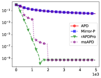
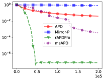
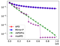
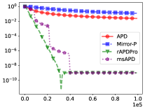
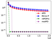
Figure 1: Results on objective convergence to optimum. Datasets (Top-Bottom-Left-Right order) correspond to bio-CE-HT, bio-CE-LC, econ-beaflw, DD68, DD242 and peking-1. The $x$-axis reports the iteration number. The $y$-axis reports $\log_{10}((\|D^{1/2}\mathbf{x}_{k}\|_{1}-\|D^{1/2}\mathbf{x}^{*}\|_{1})/\|D^{1/2}\mathbf{x}^{*}\|_{1})$ for rAPDPro, and $\log_{10}((\|D^{1/2}\bar{\mathbf{x}}_{k}\|_{1}-\|D^{1/2}\mathbf{x}^{*}\|_{1})/\|D^{1/2}\mathbf{x}^{*}\|_{1})$ for APD, msAPD and Mirror-Prox ($\mathbf{x}^{*}$ is computed by CVXPY [6]).

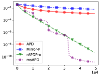
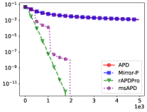
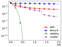
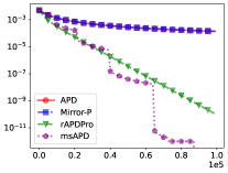
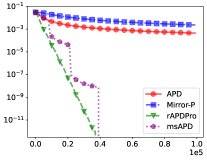
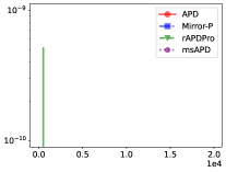
Figure 2: Results on feasibility violation. Datasets (Top-Bottom-Left-Right order) correspond to bio-CE-HT, bio-CE-LC, econ-beaflw, DD68, DD242 and peking-1. The $x$-axis reports the iteration number. The $y$-axis reports the feasibility gap $\log_{10}(\max\{0,G(\mathbf{x}_{k})\})$ for rAPDPro, and $\log_{10}(\max\{0,G(\bar{\mathbf{x}}_{k})\})$ for APD, msAPD and Mirror-Prox.

We plot the relative function value gap $|f(\mathbf{x})-f(\mathbf{x}^{*})|/|f(\mathbf{x}^{*})|$ and the feasibility violation $\max\{G(\mathbf{x}),0\}$ over the iteration number in Figure 1, 2, respectively. Firstly, in all experiments, in terms of both optimality gap and constraint violation, the performance of rAPDPro and msAPD is significantly better than that of APD and Mirror-Prox. Additionally, rAPDPro and msAPD often converge to high-precision solutions. Secondly, based on the experimental results, it is indeed observed that msAPD exhibits a periodic variation in convergence performance, which aligns with our algorithm theory.

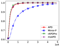
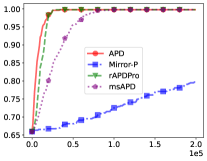
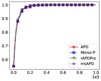
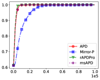
Figure 3: The experimental results on active-set identification. Datasets (Top-Bottom-Left-Right order) correspond to bio-CE-HT, bio-CE-LC, econ-beaflw, DD68, DD242 and peking-1. The $x$-axis reports the iteration number and the $y$-axis reports accuracy in active-set identification.

Next, we examine the algorithm’s effectiveness in identifying sparsity patterns. We computed a nearly optimal solution $\mathbf{x}^{*}$ from CVXPY. Note that $\mathbf{x}^{*}$ is a dense vector. For numerical consideration, we truncate the coordinate values of $\mathbf{x}^{*}$ to zero if the absolute value is below $10^{-8}$ and perform the same truncation to all the generated solutions of the compared algorithms. Then we use $(|\mathcal{A}(\mathbf{x})\cap\mathcal{A}(\mathbf{x}^{*})|+|\mathcal{A}^{c}(\mathbf{x})\cap\mathcal{A}^{c}(\mathbf{x}^{*})|)/n$ to measure the accuracy of identifying the active set, where $|\cdot|$ denotes the set cardinality. For rAPDPro, we consider the last iterate $\mathbf{x}_{k}$ while for APD, msAPD and Mirror-Prox, we plot the result on $\bar{\mathbf{x}}_{k}$, as these are the solutions where the convergence rates are established. Figure 3 plots the experiment result, from which we observe that rAPDPro and msAPD are highly effective in identifying the active set. Often, they are able to recognize the structure of the active set within a small number of iterations. While APD can identify the active set in many cases, it fails in peking-1. Overall, the experimental results show the great potential of our proposed algorithms in identifying the sparsity structure and are consistent with our theoretical analysis.

8 Conclusion

The key contribution of this paper is that we develop several new first-order primal-dual algorithms for convex optimization with strongly convex constraints. Using some novel strategies to exploit the strong convexity of the Lagrangian function, we substantially improve the best convergence rate from $\mathcal{O}(1/\varepsilon)$ to $\mathcal{O}(1/\sqrt{\varepsilon})$. In the application of constrained sparse learning problems, the experimental study confirms the advantage of our proposed algorithms against state-of-the-art first-order methods for constrained optimization. Moreover, we show that one of our proposed algorithms rAPDPro has the favorable feature of identifying the sparsity pattern in the optimal solution. For future work, one direction is to apply adaptive strategy, such as line search, to our framework for dealing with the case when dual bound is unavailable. It also would be interesting to consider a more general convex objective when the proximal operator is not easy to compute. Another interesting direction is to further exploit the active set identification property in a general setting. For example, it would be interesting to incorporate our algorithm with active constraint identification, which could be highly desirable when there are a large number of constraints.

Appendix A Auxiliary lemmas

The following three-point property is important in the convergence analysis.

Lemma 4.

Let $f:\mathbb{R}^{n}\to\mathbb{R\cup}\{+\infty\}$ be a closed strongly convex function with modulus $\mu\geq 0$. Give $\bar{\mathbf{x}}\in\mathcal{X}$, where $\mathcal{X}$ is a compact convex set and $t\geq 0$, let $\mathbf{x}^{+}=\operatornamewithlimits{argmin}_{x\in\mathcal{X}}f(\mathbf{x})+\frac{t}{2}\|\mathbf{x}-\bar{\mathbf{x}}\|^{2},$ then for all $\mathbf{x}\in\mathcal{X}$, we have

$$f(\mathbf{x})+\frac{t}{2}\|\mathbf{x}-\bar{\mathbf{x}}\|^{2}\geq f(\mathbf{x}^{+})+\frac{t+\mu}{2}\|\mathbf{x}^{+}-\mathbf{x}\|^{2}+\frac{t}{2}\|\mathbf{x}^{+}-\bar{\mathbf{x}}\|^{2}.$$

Proof.

Since $\mathcal{X}$ is a convex compact set, $\phi(x):=I_{\mathcal{X}}(\mathbf{x})+f(\mathbf{x})+\frac{t}{2}\|\mathbf{x}-\bar{\mathbf{x}}\|^{2}$ is lower-semi-continuous and $(\mu+t)$-strongly convex, where $I_{\mathcal{X}}(\mathbf{x})=\begin{cases}0&\mathbf{x}\in\mathcal{X}\\ \infty&\mathbf{x}\notin\mathcal{X}\end{cases}$. Using the optimality ($\mathbf{0}\in\phi(\mathbf{x}^{+})$) and strong convexity, we have $\phi(\mathbf{x})\geq\phi(\mathbf{x}^{+})+\langle\mathbf{0},\mathbf{x}-\mathbf{x}^{+}\rangle+\frac{t+\mu}{2}\|\mathbf{x}^{+}-\mathbf{x}\|^{2}$, for any $\mathbf{x}\in\mathcal{X}$. This immediately gives the desired relation. ∎

The following result is adjusted from the classic supermartingale convergence theorem ([27, Theorem 1]). We give proof for completeness.

Lemma 5.

Let $(\Omega,\mathcal{F},\mathbb{P})$ be a probability space and $\mathcal{F}_{1}\subset\mathcal{F}_{2}\subset\cdots$ be a sequence of sub-$\sigma$-algebras of $\mathcal{F}$. For each $j=1,2,\cdots$, let $a_{j},b_{j}$ and $c_{j}$ be non-negative $\mathcal{F}_{n}$-measure random variables such $\mathbb{E}[a_{j+1}\mid\mathcal{F}_{j}]\leq a_{j}-b_{j}+c_{j}$, then we have $\lim_{j\to\infty}a_{j}<\infty$ exists and $\sum_{j=1}^{\infty}b_{j}<\infty$ a.s. when $\sum_{j=1}^{\infty}c_{j}<\infty$.

Proof.

Define $d_{j}=a_{j}-\sum_{l=1}^{j-1}(c_{l}-b_{l})$ and for any $\bar{a}>0$, define $t=\inf\{t:\sum_{l=1}^{t}c_{l}>\bar{a}\}$. If $j<t$, we have

$$\mathbb{E}[d_{j+1}\mid\mathcal{F}_{j}]=\mathbb{E}[a_{j+1}-\sum_{l=1}^{j}(c_{l}-b_{l})\mid\mathcal{F}_{j}]\overset{(a)}{\leq}a_{j}-\sum_{l=1}^{j-1}(c_{l}-b_{l})=:d_{j},$$ (44)

where $(a)$ holds by $\mathbb{E}[a_{j+1}\mid\mathcal{F}_{j}]\leq a_{j}+c_{j}-b_{j}$, and hence

$$\mathbb{E}[d_{\min\{t,(j+1)\}}\mid\mathcal{F}_{j}]=d_{t}\mathbb{I}_{\{t\leq j\}}+\mathbb{E}[d_{j+1}\mid\mathcal{F}_{j}]\mathbb{I}_{\{t>j\}}\overset{(a)}{\leq}d_{\min\{t,j\}},$$

where $(a)$ holds by (44). Therefore, we have $\{d_{\min\{t,(j+1)\}},\mathcal{F}_{j},1\leq j\leq\infty\}$ is a supermartingale. Since

$$d_{\min\{t,j\}}=a_{\min\{t,j\}}-\sum_{l=1}^{\min\{t,j\}-1}(c_{l}-b_{l})\overset{(a)}{\geq}-\sum_{l=1}^{\min\{t,(j-1)\}}c_{l}\geq-\bar{a},$$

holds for all $j$, where $(a)$ holds by $a_{\min\{t,j\}},b_{l}\geq 0$. Then it follows from the martingale convergence theorem that $\lim_{j\to\infty}d_{\min\{t,j\}}$ exists and is finite a.s., i.e., $\lim_{j\to\infty}d_{j}$ exists and is finite on $\{t=\infty\}=\{\sum_{j=1}^{\infty}c_{j}\leq\bar{a}\}$. Since $\bar{a}$ is arbitrary, we see that $\lim_{j\to\infty}d_{j}$ exists and is finite a.s. on $\{\sum_{j=1}^{\infty}c_{j}<\infty\}$. By $d_{j}=a_{j}-\sum_{l=1}^{j-1}(c_{l}-b_{l})$, we have $\lim_{j\to\infty}a_{j}$ exists and is finite and $\sum_{j=1}^{\infty}b_{j}<\infty$ when $\{\sum_{j=1}^{\infty}c_{j}<\infty\}$. ∎

Appendix B Proof details in Section 3

B.1 Proof of Theorem 1

Proof.

First, it is easy to verify by our construction that $\{\mathcal{Y}_{k}\}$ is a monotone sequence: $\mathcal{Y}_{1}\supseteq\mathcal{Y}_{2}\supseteq\ldots\supseteq\mathcal{Y}_{k}\ldots$. Our goal is to show $\mathcal{Y}^{*}\subseteq\mathcal{Y}_{k}$ holds for any $k\geq 0$ by induction. Note that $\mathcal{Y}^{*}\subseteq\mathcal{Y}_{0}$ immediately follows from our assumption that $(\mathbf{y}^{*})^{\top}\bm{\mu}\geq\rho_{0}$, for any $\mathbf{y}^{*}\in\mathcal{Y}^{*}$. Suppose that $\mathcal{Y}^{*}\subseteq\mathcal{Y}_{k}$ holds for $k=0,\ldots,K-1$, we claim:

1. For any $\mathbf{x}\in\mathcal{X}$ and $\mathbf{y}\in\mathcal{Y}^{*}$, we have

   $$\mathcal{L}(\bar{\mathbf{x}}_{K},\mathbf{y})-\mathcal{L}(\mathbf{x},\bar{\mathbf{y}}_{K})\leq\frac{1}{T_{K}}\Delta(\mathbf{x},\mathbf{y})-\frac{t_{K-1}\tau_{K-1}^{-1}}{2T_{K}}\|\mathbf{x}-\mathbf{x}_{K}\|^{2}.$$ (45)

2. $\mathcal{Y}^{*}\subseteq\mathcal{Y}_{K}$.

Part 1. For $k=0,1,2,\ldots,K-1$, taking $-\left\langle\mathbf{z}_{k},\cdot\right\rangle$ and $f(\cdot)+\left\langle\nabla G(\mathbf{x}_{k})\mathbf{y}_{k+1},\cdot\right\rangle$ in Lemma 4, the following relations

$$-\langle\mathbf{y}_{k+1}-\mathbf{y},\mathbf{z}_{k}\rangle \leq A_{k+1},$$ (46)

$$f(\mathbf{x}_{k+1})+\left\langle\mathbf{y}_{k+1},\nabla G(\mathbf{x}_{k})^{\top}(\mathbf{x}_{k+1}-\mathbf{x})\right\rangle \leq f(\mathbf{x})+B_{k+1},$$ (47)

where

$$A_{k+1} \triangleq\frac{1}{2\sigma_{k}}\left(\|\mathbf{y}-\mathbf{y}{}_{k}\|^{2}-\|\mathbf{y}-\mathbf{y}_{k+1}\|^{2}-\|\mathbf{y}_{k+1}-\mathbf{y}_{k}\|^{2}\right),$$ (48)

$$B_{k+1} \triangleq\frac{1}{2\tau_{k}}\left(\|\mathbf{x}-\mathbf{x}_{k}\|^{2}-\|\mathbf{x}-\mathbf{x}_{k+1}\|^{2}-\|\mathbf{x}_{k+1}-\mathbf{x}_{k}\|^{2}\right),$$ (49)

hold for any $\mathbf{x}\in\mathcal{X}$ and $\mathbf{y}\in\bigcap_{0\leq s\leq k}\mathcal{Y}_{s}$. The existence of such $\mathbf{y}$ follows from our induction hypothesis. Since $\mathbf{y}_{k+1}^{\top}G(\cdot)$ is $\rho_{k}$-strongly convex, we have

$$\left\langle\mathbf{y}_{k+1},\nabla G(\mathbf{x}_{k})^{\top}(\mathbf{x}_{k+1}-\mathbf{x})\right\rangle$$

$$\geq{}\left\langle\mathbf{y}_{k+1},\nabla G(\mathbf{x}_{k})^{\top}(\mathbf{x}_{k+1}-\mathbf{x}_{k})\right\rangle$$

$$\ \ +\left\langle\mathbf{y}_{k+1},G(\mathbf{x}_{k+1})-G(\mathbf{x})\right\rangle-\left\langle\mathbf{y}_{k+1},G(\mathbf{x}_{k+1})-G(\mathbf{x}_{k})\right\rangle+\frac{\rho_{k}}{2}\|\mathbf{x}-\mathbf{x}_{k}\|^{2}.$$

Combining this result and (47), we have

$$\begin{split}&f(\mathbf{x}_{k+1})-f(\mathbf{x})+\left\langle\mathbf{y}_{k+1},G(\mathbf{x}_{k+1})-G(\mathbf{x})\right\rangle\\ &\leq{}B_{k+1}-\left\langle\mathbf{y}_{k+1},\nabla G(\mathbf{x}_{k})^{\top}(\mathbf{x}_{k+1}-\mathbf{x}_{k})\right\rangle+\left\langle\mathbf{y}_{k+1},G(\mathbf{x}_{k+1})-G(\mathbf{x}_{k})\right\rangle-\frac{\rho_{k}}{2}\|\mathbf{x}-\mathbf{x}_{k}\|^{2}.\end{split}$$ (50)

On the other hand, by the definition of $\mathbf{z}_{k}$, we have

$$\langle\mathbf{y}-\mathbf{y}_{k+1},\mathbf{z}_{k}\rangle$$

$$={}\langle\mathbf{y}-\mathbf{y}_{k+1},G(\mathbf{x}_{k})-G(\mathbf{x}_{k+1})\rangle+\langle\mathbf{y}-\mathbf{y}_{k+1},G(\mathbf{x}_{k+1})\rangle$$ (51)

$$\ \ +\theta_{k}\langle\mathbf{y}-\mathbf{y}_{k},G(\mathbf{x}_{k})-G(\mathbf{x}_{k-1})\rangle+\theta_{k}\langle\mathbf{y}_{k}-\mathbf{y}_{k+1},G(\mathbf{x}_{k})-G(\mathbf{x}_{k-1})\rangle.$$

Let us denote $\mathbf{q}_{k}=G(\mathbf{x}_{k})-G(\mathbf{x}_{k-1})$ for brevity. Combining (46) and (51) yields

$$\begin{split}&\langle\mathbf{y}-\mathbf{y}_{k+1},G(\mathbf{x}_{k+1})\rangle\\ &\leq A_{k+1}+\langle\mathbf{y}-\mathbf{y}_{k+1},G(\mathbf{x}_{k+1})-G(\mathbf{x}_{k})\rangle-\theta_{k}\langle\mathbf{y}-\mathbf{y}_{k},\mathbf{q}_{k}\rangle-\theta_{k}\langle\mathbf{y}_{k}-\mathbf{y}_{k+1},\mathbf{q}_{k}\rangle.\end{split}$$ (52)

Putting (50) and (52) together, we have

$$\mathcal{L}(\mathbf{x}_{k+1},\mathbf{y})-\mathcal{L}(\mathbf{x},\mathbf{y}_{k+1})$$

$$\leq{}A_{k+1}+B_{k+1}-\left\langle\mathbf{y}_{k+1},\nabla G(\mathbf{x}_{k})^{\top}(\mathbf{x}_{k+1}-\mathbf{x}_{k})\right\rangle+\left\langle\mathbf{y}_{k+1},G(\mathbf{x}_{k+1})-G(\mathbf{x}_{k})\right\rangle$$

$$\ \ +\langle\mathbf{y}-\mathbf{y}_{k+1},\mathbf{q}_{k+1}\rangle-\theta_{k}\langle\mathbf{y}-\mathbf{y}_{k},\mathbf{q}_{k}\rangle+\theta_{k}\langle\mathbf{y}_{k+1}-\mathbf{y}_{k},\mathbf{q}_{k}\rangle-\frac{\rho_{k}}{2}\|\mathbf{x}-\mathbf{x}_{k}\|^{2}$$

$$\leq{}A_{k+1}+B_{k+1}+\frac{L_{XY}}{2}\|\mathbf{x}_{k+1}-\mathbf{x}_{k}\|^{2}-\frac{\rho_{k}}{2}\|\mathbf{x}-\mathbf{x}_{k}\|^{2}$$

$$\ \ +\langle\mathbf{y}-\mathbf{y}_{k+1},\mathbf{q}_{k+1}\rangle-\theta_{k}\langle\mathbf{y}-\mathbf{y}_{k},\mathbf{q}_{k}\rangle+\theta_{k}\langle\mathbf{y}_{k+1}-\mathbf{y}_{k},\mathbf{q}_{k}\rangle,$$

where the last inequality is by Lipschitz smoothness of $\left\langle\mathbf{y}_{k+1},G(\cdot)\right\rangle$.

Next, we bound the term $\langle\mathbf{q}_{k},\mathbf{y}_{k+1}-\mathbf{y}_{k}\rangle$ by Young’s inequality, which gives

$$\begin{split}\langle\mathbf{y}_{k+1}-\mathbf{y}_{k},\mathbf{q}_{k}\rangle&\leq\frac{\delta}{2\sigma_{k-1}}\|\mathbf{y}_{k+1}-\mathbf{y}_{k}\|^{2}+\frac{\sigma_{k-1}}{2\delta}\|\mathbf{q}_{k}\|^{2},\end{split}$$ (53)

where $\delta$ is a positive constant. It follows from (53) and $\frac{\sigma_{k}}{2\delta}\|\mathbf{q}_{k+1}\|^{2}\leq\frac{L_{G}^{2}\sigma_{k}}{2\delta}\|\mathbf{x}_{k+1}-\mathbf{x}_{k}\|^{2}$ that

$$\mathcal{L}(\mathbf{x}_{k+1},\mathbf{y})-\mathcal{L}(\mathbf{x},\mathbf{y}_{k+1})$$ (54)

$$\leq\frac{\tau_{k}^{-1}-\rho_{k}}{2}\|\mathbf{x}-\mathbf{x}_{k}\|^{2}-\frac{\tau_{k}^{-1}}{2}\|\mathbf{x}-\mathbf{x}_{k+1}\|^{2}+\frac{\theta_{k}\sigma_{k-1}}{2\delta}\|\mathbf{q}_{k}\|^{2}-\frac{\sigma_{k}}{2\delta}\|\mathbf{q}_{k+1}\|^{2}$$

$$\ \ +\frac{1}{2\sigma_{k}}\left(\|\mathbf{y}-\mathbf{y}{}_{k}\|^{2}-\|\mathbf{y}-\mathbf{y}_{k+1}\|^{2}\right)+\langle\mathbf{y}-\mathbf{y}_{k+1},\mathbf{q}_{k+1}\rangle-\theta_{k}\langle\mathbf{y}-\mathbf{y}_{k},\mathbf{q}_{k}\rangle$$

$$\ \ -\frac{\sigma_{k}^{-1}-\theta_{k}\delta/\sigma_{k-1}}{2}\|\mathbf{y}_{k+1}-\mathbf{y}_{k}\|^{2}+\frac{L_{G}^{2}\sigma_{k}}{2\delta}\|\mathbf{x}_{k+1}-\mathbf{x}_{k}\|^{2}-\frac{\tau_{k}^{-1}-L_{XY}}{2}\|\mathbf{x}_{k+1}-\mathbf{x}_{k}\|^{2}.$$

Multiply both sides of the above relation by $t_{k}$ and sum up the result for $k=0,1,\ldots,K-1$. In view of the parameter relation (14) and (15), we have

$$\sum_{k=0}^{K-1}t_{k}\big{[}\mathcal{L}(\mathbf{x}_{k+1},\mathbf{y})-\mathcal{L}(\mathbf{x},\mathbf{y}_{k+1})\big{]}$$

$$\overset{(a)}{\leq}\frac{t_{0}(\tau_{0}^{-1}-\rho_{0})}{2}\|\mathbf{x}-\mathbf{x}_{0}\|^{2}-\frac{t_{K-1}\tau_{K-1}^{-1}}{2}\|\mathbf{x}-\mathbf{x}_{K}\|^{2}-\frac{t_{K-1}\sigma_{k-1}}{2\delta}\|\mathbf{q}_{K}\|^{2}$$

$$\quad+\frac{t_{0}\sigma_{0}^{-1}}{2}\|\mathbf{y}-\mathbf{y}_{0}\|^{2}-\frac{t_{K-1}\sigma_{K-1}^{-1}}{2}\|\mathbf{y}-\mathbf{y}_{K}\|^{2}+t_{K-1}\langle\mathbf{y}-\mathbf{y}_{K},\mathbf{q}_{K}\rangle-t_{0}\theta_{0}\langle\mathbf{y}-\mathbf{y}_{0},\mathbf{q}_{0}\rangle$$

$$\overset{(b)}{\leq}\frac{1}{2\tau_{0}}\|\mathbf{x}-\mathbf{x}_{0}\|^{2}+\frac{1}{2\sigma_{0}}\|\mathbf{y}-\mathbf{y}_{0}\|^{2}-\frac{t_{K-1}\tau_{K-1}^{-1}}{2}\|\mathbf{x}-\mathbf{x}_{K}\|^{2}-\frac{(1-\delta)t_{K-1}\sigma_{K-1}^{-1}}{2}\|\mathbf{y}-\mathbf{y}_{K}\|^{2},$$

where $(a)$ uses $\mathbf{q}_{0}=\bm{0}$ and $\mathbf{x}_{-1}=\mathbf{x}_{0}$, and $(b)$ holds by $\rho_{0}=0$, $t_{0}=1$ and

$$t_{K-1}\left\langle\mathbf{y}-\mathbf{y}_{K},\mathbf{q}_{K}\right\rangle\leq\frac{t_{K-1}\delta}{2\sigma_{K-1}}\|\mathbf{y}-\mathbf{y}_{K}\|^{2}+\frac{t_{K-1}}{2\delta/\sigma_{K-1}}\|\mathbf{q}_{K}\|^{2}.$$

Since $\mathcal{L}(\mathbf{x},\mathbf{y})$ is convex in $\mathbf{x}$ and linear in $\mathbf{y}$, we have

$$T_{K}\big{[}\mathcal{L}(\bar{\mathbf{x}}_{K},\mathbf{y})-\mathcal{L}(\mathbf{x},\bar{\mathbf{y}}_{K})\big{]}\leq\sum_{k=0}^{K-1}t_{k}\big{[}\mathcal{L}(\mathbf{x}_{k+1},\mathbf{y})-\mathcal{L}(\mathbf{x},\mathbf{y}_{k+1})\big{]},$$ (55)

Combining (B.1) and (55), we obtain

$$T_{K}\big{[}\mathcal{L}(\bar{\mathbf{x}}_{K},\mathbf{y})-\mathcal{L}(\mathbf{x},\bar{\mathbf{y}}_{K})\big{]}\leq \frac{1}{2\tau_{0}}\|\mathbf{x}-\mathbf{x}_{0}\|^{2}-\frac{t_{K-1}\tau_{K-1}^{-1}}{2}\|\mathbf{x}-\mathbf{x}_{K}\|^{2}$$ (56)

$$+\frac{1}{2\sigma_{0}}\|\mathbf{y}-\mathbf{y}_{0}\|^{2}-\frac{(1-\delta)t_{K-1}\sigma_{K-1}^{-1}}{2}\|\mathbf{y}-\mathbf{y}_{K}\|^{2}.$$

Dividing both sides by $T_{K},$ we obtain the desired result (45).

Part 2. Next we show $\mathcal{Y}^{*}\subseteq\mathcal{Y}_{K}$. Let $\mathbf{y}^{*}$ be any point in $\mathcal{Y}^{*}$. Since (56) holds for any $\mathbf{x}\in\mathcal{X}$ and $\mathbf{y}\in\cap_{0\leq k\leq K-1}\mathcal{Y}_{k}\supseteq\mathcal{Y}^{*}$, we can place $\mathbf{x}=\mathbf{x}^{*},\mathbf{y}=\mathbf{y}^{*}\in\mathcal{Y}^{*}$ in (45) to obtain

$$\frac{t_{K-1}\tau_{K-1}^{-1}}{2T_{K}}\|\mathbf{x}^{*}-\mathbf{x}_{K}\|^{2}+\mathcal{L}(\bar{\mathbf{x}}_{K},\mathbf{y}^{*})-\mathcal{L}(\mathbf{x}^{*},\bar{\mathbf{y}}_{K})\leq\frac{1}{T_{K}}\Delta(\mathbf{x}^{*},\mathbf{y}^{*}).$$

Moreover, the strong convexity of $\mathcal{L}(\cdot,\mathbf{y}^{*})$ implies

$$\mathcal{L}(\bar{\mathbf{x}}_{K},\mathbf{y}^{*})\geq\mathcal{L}(\mathbf{x}^{*},\mathbf{y}^{*})+\frac{(\mathbf{y}^{*})^{\top}\bm{\mu}}{2}\|\bar{\mathbf{x}}_{K}-\mathbf{x}^{*}\|^{2}\geq\mathcal{L}(\mathbf{x}^{*},\bar{\mathbf{y}}_{K})+\frac{(\mathbf{y}^{*})^{\top}\bm{\mu}}{2}\|\bar{\mathbf{x}}_{K}-\mathbf{x}^{*}\|^{2}.$$

Applying the above two inequalities yields

$$\frac{(\mathbf{y}^{*})^{\top}\bm{\mu}}{2}\|\bar{\mathbf{x}}_{K}-\mathbf{x}^{*}\|^{2}\leq\frac{1}{T_{K}}\Delta(\mathbf{x}^{*},\mathbf{y}^{*}),\ \frac{1}{2}\|\mathbf{x}_{K}-\mathbf{x}^{*}\|^{2}\leq\frac{\tau_{K-1}\sigma_{0}}{\sigma_{K-1}}\Delta(\mathbf{x}^{*},\mathbf{y}^{*}).$$ (57)

In view of (57) and Proposition 4, we have that

$$(\mathbf{y}^{*})^{T}\bm{\mu}\geq\underline{\mu}\,\|\mathbf{y}^{*}\|_{1}=\underline{\mu}\max\big{\{}h_{1}(\mathbf{x}_{K},\frac{\sigma_{0}\tau_{K-1}\Delta_{XY}}{\sigma_{K-1}}),h_{2}(\bar{\mathbf{x}}_{K},\frac{\Delta_{XY}}{T_{K}})\big{\}}:=\hat{\rho}_{K}.$$

Moreover, since $\mathcal{Y}^{*}\subseteq\mathcal{Y}_{K-1}$, we have $(\mathbf{y}^{*})^{T}\bm{\mu}\geq\rho_{K-1}$. Hence we have $(\mathbf{y}^{*})^{T}\bm{\mu}\geq\rho_{K}$ where $\rho_{K}=\max\{\hat{\rho}_{K},\rho_{K-1}\}$ is the output of the Improve procedure. Due to the construction of $\mathcal{Y}_{K}$, we immediately see that $\mathbf{y}^{*}\in\mathcal{Y}_{K}$. This implies $\mathcal{Y}^{*}\subseteq\mathcal{Y}_{K}$ and completes our induction proof. ∎

B.2 Proof of Corollary 1

Proof.

First, we show that the sequences $\{\tau_{k},\sigma_{k},t_{k},\theta_{k},\rho_{k}\}$ generated by APDPro satisfy the relationship in (14) and (15) in Theorem 1. The first part of (14) can be derived using the monotonicity of $\{\rho_{k}\}$ and $\{\gamma_{k}\}$ as follows:

$$t_{k+1}(\tau_{k+1}^{-1}-\rho_{k+1})=\sigma_{0}^{-1}(\gamma_{k}+\gamma_{k}\rho_{k+1}\tau_{k}-\sqrt{\gamma_{k+1}\gamma_{k}}\rho_{k+1}\tau_{k})\leq\sigma_{0}^{-1}\gamma_{k}=t_{k}\tau_{k}^{-1}.$$

The rest of (14) can be easily verified using the parameters setting (18).

Next, we prove the first term in (15) by induction. Firstly, it easy to verify that for any $\sigma_{0}>0$, there exists $\tau_{0}\in(0,(L_{XY}+L_{G}^{2}\sigma_{0}/\delta)^{-1}]$ such that (17) holds. Hence, when $k=0$, the first term in (15) is directly from (17). Suppose that the first inequality in (15) holds for $k=0,\ldots,K-1$. From $\theta_{K}={\sigma_{K-1}}/{\sigma_{K}}={\tau_{K}}/{\tau_{K-1}}\leq 1$, we have

$$\frac{1}{\tau_{K}}=\frac{1}{\tau_{K-1}\theta_{K}}\geq\frac{L_{XY}}{\theta_{K}}+\frac{L_{G}^{2}\sigma_{K-1}\delta^{-1}}{\theta_{K}}\geq L_{XY}+L_{G}^{2}\sigma_{K}\delta^{-1}.$$ (58)

Without loss of generality, place $\mathbf{x}=\mathbf{x}^{*}$, $\mathbf{y}=\mathbf{y}^{+}:=\left(\|\mathbf{y}^{*}\|_{1}+c^{*}\right)\frac{[G(\bar{\mathbf{x}}_{K})]_{+}}{\|[G(\bar{\mathbf{x}}_{K})]_{+}\|}$ in (45), and using $\|\mathbf{y}^{*}\|_{1}\leq\bar{c}$ in Proposition 1. It is easy to see $\|\mathbf{y}^{+}\|=\|\mathbf{y}^{*}\|_{1}+c^{*}\leq\bar{c}$, and $\|\mathbf{y}^{+}\|_{1}\geq\|\mathbf{y}^{+}\|=\|\mathbf{y}^{*}\|_{1}+c^{*}\geq\|\mathbf{y}^{*}\|_{1},$ Hence, we conclude that $\mathbf{y}^{+}\in\mathcal{Y}_{k},\forall k\geq 0$.

Now observe that $\mathcal{L}(\bar{\mathbf{x}}_{K},\mathbf{y}^{*})-\mathcal{L}(\mathbf{x}^{*},\mathbf{y}^{*})\geq 0$, which implies that

$$f(\bar{\mathbf{x}}_{K})+\left\langle\mathbf{y}^{*},G(\bar{\mathbf{x}}_{K})\right\rangle-f(\mathbf{x}^{*})\geq 0.$$

In view of $\left\langle\mathbf{y}^{*},G(\bar{\mathbf{x}}_{K})\right\rangle\leq\left\langle\mathbf{y}^{*},[G(\bar{\mathbf{x}}_{K})]_{+}\right\rangle\leq\|\mathbf{y}^{*}\|\cdot\|[G(\bar{\mathbf{x}}_{K})]_{+}\|$, then we have

$$f(\bar{\mathbf{x}}_{K})+\|\mathbf{y}^{*}\|\cdot\|[G(\bar{\mathbf{x}}_{K})]_{+}\|-f(\mathbf{x}^{*})\geq 0.$$ (59)

Moreover, it follows that $\|\mathbf{y}^{*}\|_{1}\geq\|\mathbf{y}^{*}\|$ that

$$\begin{split}\mathcal{L}(\bar{\mathbf{x}}_{K},\mathbf{y}^{+})-\mathcal{L}(\mathbf{x}^{*},\bar{\mathbf{y}}_{K})&\geq\mathcal{L}(\bar{\mathbf{x}}_{K},\mathbf{y}^{+})-\mathcal{L}(\mathbf{x}^{*},\mathbf{y}^{*})\\ &\geq f(\bar{\mathbf{x}}_{K})+\left(\|\mathbf{y}^{*}\|+c^{*}\right)\|[G(\bar{\mathbf{x}}_{K})]_{+}\|-f(\mathbf{x}^{*}).\end{split}$$ (60)

Combining (59), (60) and (45), we obtain

$$\max\big{\{}c^{*}\|[G(\bar{\mathbf{x}}_{K})]_{+}\|,f(\bar{\mathbf{x}}_{K})-f(\mathbf{x}^{*})\big{\}}\leq{\frac{1}{T_{K}}\big{(}\frac{1}{2\tau_{0}}\|\mathbf{x}_{0}-\mathbf{x}^{*}\|^{2}+\frac{D_{Y}^{2}}{2\sigma_{0}}\big{)}},$$ (61)

In view of the bound in (20) and the relation between $\tau_{k},\sigma_{k},T_{k}$, we can get

$$\frac{\tau_{k}}{\sigma_{k}}\leq\frac{3}{\hat{\rho}_{k}^{2}\tau_{0}^{2}k^{2}+9\gamma_{0}}.$$ (62)

In view of (61) and (20), we have

$$\max\big{\{}c^{*}\|[G(\bar{\mathbf{x}}_{K})]_{+}\|,f(\bar{\mathbf{x}}_{K})-f(\mathbf{x}^{*})\big{\}}\leq\frac{6}{6+\tau_{0}\tilde{\rho}_{K}(K+1)K}{\big{(}\frac{1}{2\tau_{0}}\|\mathbf{x}_{0}-\mathbf{x}^{*}\|^{2}+\frac{D_{Y}^{2}}{2\sigma_{0}}\big{)}}.$$

Combining (45) and (62) yields $\frac{1}{2}\|\mathbf{x}_{K}-\mathbf{x}^{*}\|^{2}\leq{3\sigma_{0}}{\Delta(\mathbf{x}^{*},\mathbf{y}^{*})}/({\hat{\rho}_{K}^{2}\tau_{0}^{2}K^{2}+9\gamma_{0}}).$ ∎

Appendix C Proof details in Section 4

C.1 Proof of Lemma 2

Proof.

First, we give some results that will be used in the following repeatedly. In view of Lemma 1, and the parameter ergodic sequence generated by rAPDPro, we have $\left\{(\tau_{k}^{s})^{-1},\sigma_{k}^{s}\right\}$ is monotonically increasing sequence in $k$, $\bar{\tau}={\tau_{0}^{s}},\bar{\sigma}={\sigma_{0}^{s}},\theta_{0}^{s}=1,t_{0}^{s}=1,\forall s\geq 0$, and there exist a $\nu_{3}>0$ such that $\bar{\sigma}+\nu_{3}\leq\underline{\sigma}:=\min_{s}\{\sigma_{N_{s}}^{s}\}$. Now, for rAPDPro, we claim that there exist $\nu_{1},\nu_{2}>0$ such that the following two conditions hold

1. For any $j\geq 0$, we have

$$\min\big{\{}(\sigma_{j}^{-1}-\theta_{j}\delta/\sigma_{j-1})\sigma_{j},(\tau_{j}^{-1}-L_{XY}-L_{G}^{2}\sigma_{j}/\delta)\tau_{j}\big{\}}\geq\nu_{1}>0,$$ (63)

and

$$\begin{split}t_{j}\min\Big{\{}\tau_{j}^{-1}-\rho_{j},\frac{1}{\sigma_{j}}-\frac{\delta}{\sigma_{j-1}}\Big{\}}&\geq\nu_{2}>0.\end{split}$$ (64)

2. For any $j\geq 0$, we have

$$0\leq t_{j}Q_{j}(\mathbf{x}^{*},\tilde{\mathbf{y}}^{*})-t_{j+1}Q_{j+1}(\mathbf{x}^{*},\tilde{\mathbf{y}}^{*})-\nu_{1}t_{j}\big{(}{(2\tau_{j})^{-1}}\|\mathbf{x}_{j+1}-\mathbf{x}_{j}\|^{2}+{(2\sigma_{j})^{-1}}\|\mathbf{y}_{j+1}-\mathbf{y}_{j}\|^{2}\big{)}.$$ (65)

Part 1. We first consider two subsequent points $\mathbf{x}_{j}$ and $\mathbf{x}_{j+1}$ within the same epoch, and assume $j\sim(s,k)$. Then, it follows from $\theta_{k}^{s}={\sigma_{k-1}^{s}}/{\sigma_{k}^{s}}$ that

$$(\sigma_{k}^{s})^{-1}-\theta_{k}^{s}\delta(\sigma_{k-1}^{s})^{-1}=(\sigma_{k}^{s})^{-1}-\delta(\sigma_{k}^{s})^{-1}=\frac{1-\delta}{\sigma_{k}^{s}}\overset{\eqref{eq:ini_step_assu}}{\geq}\frac{\nu_{0}}{\sigma_{k}^{s}}.$$ (66)

Next, we use induction to show

$$\frac{1-\nu_{0}}{\tau_{k}^{s}}\geq L_{XY}+L_{G}^{2}\sigma_{k}^{s}\delta^{-1}.$$ (67)

When $k=0$, inequality (67) degenerates as the definition of $\tau_{0}^{s},\sigma_{0}^{s}$. Suppose (67) holds for $k=0,1,\ldots,K-1$. Then, from $\theta_{K}^{s}={\sigma_{K-1}^{s}}/{\sigma_{K}^{s}}={\tau_{K}^{s}}/{\tau_{K-1}^{s}}\leq 1$, we have

$$(1-\nu_{0})(\tau_{K}^{s})^{-1}=(1-\nu_{0})(\tau_{K-1}^{s}\theta_{K}^{s})^{-1}\geq\frac{L_{XY}}{\theta_{K}^{s}}+\frac{L_{G}^{2}\sigma_{K-1}^{s}\delta^{-1}}{\theta_{K}^{s}}\geq L_{XY}+L_{G}^{2}\sigma_{K}^{s}\delta^{-1},$$

which completes our induction proof. Hence, combining (66) and (67), we have

$$\min\big{\{}(\sigma_{k}^{s}-\theta_{k}^{s}\delta/\sigma_{k-1}^{s})\sigma_{k}^{s},\big{(}(\tau_{k}^{s})^{-1}-L_{XY}-L_{G}^{2}\sigma^{s}_{k}/\delta\big{)}\tau_{k}^{s}\big{\}}\geq\nu_{0},\ \ \forall k\in[N_{s}].$$ (68)

Furthermore, when switching to the next epoch $(s\to s+1)$, we have

$$\begin{split}\sigma_{0}^{s+1}((\sigma_{0}^{s+1})^{-1}-\theta_{0}^{s+1}\delta/\sigma_{N_{s}}^{s})\overset{(a)}{\geq}\sigma_{0}^{s+1}((\sigma_{0}^{s+1})^{-1}-(\sigma_{N_{s}}^{s})^{-1})&\overset{(b)}{\geq}1-\sigma_{0}^{s+1}\underline{\sigma}^{-1}=1-\bar{\sigma}\underline{\sigma}^{-1}\\ ((\tau_{0}^{s+1})^{-1}-L_{XY}-L_{G}^{2}\delta^{-1}\sigma_{0}^{s+1})\tau_{0}^{s+1}&\overset{(c)}{\geq}\nu_{0}\tau_{0}^{s+1}=\nu_{0}\bar{\tau},\end{split}$$ (69)

where $(a)$ holds by $\theta_{0}^{s}=1$, $\delta<1$, $(b)$ follows from $(\sigma_{N_{s}}^{s})^{-1}\geq\underline{\sigma}^{-1}$. Hence, combining (66),  (68) and (69), we completes our proof of (63) by setting $\nu_{1}=\min\{1-\bar{\sigma}\underline{\sigma}^{-1},\nu_{0}\bar{\tau},\nu_{0}\}$.

Since rAPDPro reset the stepsize periodically and $\{t_{k}^{s},(\tau_{k}^{s})^{-1}\}_{k\in[N_{s}]}$ are two monotonically increasing sequences, hence

$$\inf_{j\geq 0}t_{j}({\tau_{j}^{-1}}-\rho_{j})\geq t_{0}^{s}({\bar{\tau}^{-1}}-\overline{\rho})=\bar{\tau}^{-1}-\overline{\rho}.$$ (70)

Consider $\inf_{k\in[N_{s}]}t_{k}^{s}\sigma_{k}^{s}(1-\delta{\sigma_{k}^{s}}/{\sigma_{k-1}^{s}})$. Combining $\delta+\nu_{0}\leq\inf_{k\in[N_{s}]}\{\theta_{k}^{s}\}$, then

$$\inf_{k\in[N_{s}]}t_{k}^{s}\sigma_{k}^{s}(1-\delta\frac{\sigma_{k}^{s}}{\sigma_{k-1}^{s}})=\inf_{k\in[N_{s}]}t_{k}^{s}\sigma_{k}^{s}(1-\delta/\theta_{k}^{s})\geq\nu_{0}\bar{\sigma}.$$ (71)

Furthermore, when switching to the next epoch $(s\to s+1)$, we have

$$\inf_{s\geq 0}t_{0}^{s+1}\sigma_{0}^{s+1}(1-\delta\sigma_{0}^{s+1}(\sigma_{N_{s}}^{s})^{-1})=\bar{\sigma}^{2}\inf_{s\geq 0}(\bar{\sigma}^{-1}-\delta(\sigma_{N_{s}}^{s})^{-1})\geq\bar{\sigma}(1-\delta),$$ (72)

where the last inequality holds by $\bar{\sigma}=\sigma_{0}^{s}\leq\sigma_{N_{s}}^{s}$. Hence, it follows from (70), (71) and (72) that there exist $\nu_{2}=\min\{\bar{\tau}^{-1}-\overline{\rho},\nu_{0}\bar{\sigma},\bar{\sigma}(1-\delta)\}$ such (64) holds.

Part 2. for any $j\geq 0,$ we have

$$\begin{split}t_{j+1}Q_{j+1}(\mathbf{x}^{*},\tilde{\mathbf{y}}^{*})&\leq t_{j}\big{(}\frac{(\tau_{j})^{-1}}{2}\|\mathbf{x}^{*}-\mathbf{x}_{j+1}\|^{2}+\left\langle G(\mathbf{x}_{j+1})-G(\mathbf{x}_{j}),\mathbf{y}_{j+1}-\tilde{\mathbf{y}}^{*}\right\rangle\\ &\ \ +{(2\sigma_{j})^{-1}}\|\tilde{\mathbf{y}}^{*}-\mathbf{y}_{j+1}\|^{2}+\frac{\sigma_{j}}{2\delta}\|G(\mathbf{x}_{j+1})-G(\mathbf{x}_{j})\|^{2}\big{)}.\end{split}$$ (73)

Consider $k\in\{0,1,\ldots,N_{s}\}$. Inequality (31) implies (14) and (15) hold (see proof of Corollary 1 in Section B.2). Hence, for $0\leq k\leq N_{s},$ we have

$$\begin{split}t_{j+1}Q_{j+1}(\mathbf{x}^{*},\tilde{\mathbf{y}}^{*})&\leq t_{k}^{s}\big{(}\frac{(\tau_{k}^{s})^{-1}}{2}\|\mathbf{x}^{*}-\mathbf{x}_{k+1}^{s}\|^{2}+\left\langle G(\mathbf{x}_{k+1}^{s})-G(\mathbf{x}_{k}^{s}),\mathbf{y}_{k+1}^{s}-\tilde{\mathbf{y}}^{*}\right\rangle\\ &\ \ +\frac{1}{2\sigma_{k}^{s}}\|\tilde{\mathbf{y}}^{*}-\mathbf{y}_{k+1}^{s}\|^{2}+\frac{\sigma_{k}^{s}}{2\delta}\|G(\mathbf{x}_{k+1}^{s})-G(\mathbf{x}_{k}^{s})\|^{2}\big{)}\end{split}$$ (74)

where $j$ corresponds to $(s,k)$. Furthermore, consider switching to next epoch $(s\to s+1)$. Since $t_{k}^{s}(\tau_{k}^{s})^{-1}$ is an increasing sequence in $k$, $\rho_{0}^{s+1}>0,t_{0}^{s+1}=1$, hence

$$t_{N_{s}}^{s}(\tau_{N_{s}}^{s})^{-1}\geq t_{0}^{s+1}(\tau_{0}^{s+1})^{-1}-\rho_{0}^{s+1}t_{0}^{s+1},\forall s\geq 0.$$ (75)

Next, we have

$$\frac{t_{N_{s}}^{s}}{\sigma_{N_{s}}^{s}}\overset{(a)}{=}\frac{t_{0}^{s+1}}{\sigma_{0}^{s+1}},\ t_{N_{s}}^{s}\overset{(b)}{\geq}t_{0}^{s+1}\overset{(c)}{=}t_{0}^{s+1}\theta_{0}^{s+1},t_{N_{s}}^{s}\sigma_{N_{s}}^{s}\overset{(b)}{\geq}t_{0}^{s+1}\sigma_{0}^{s+1}\overset{(c)}{=}t_{0}^{s+1}\sigma_{0}^{s+1}\theta_{0}^{s+1},$$ (76)

where $(a)$ holds by the definition of $t_{k}^{s}=\frac{\sigma_{k}^{s}}{\sigma_{0}^{s}}$, $(b)$ holds by $\{t_{k}^{s},\sigma_{k}^{s}\}$ is an increasing sequence in $k$, and $(c)$ holds by $\theta_{0}^{s+1}=1$. Hence, by (75) and (76), we have

$$\begin{split}t_{j+1}Q_{j+1}(\mathbf{x}^{*},\tilde{\mathbf{y}}^{*})&\leq t_{N_{s}}^{s}\big{(}\frac{1}{2\tau_{N_{s}}^{s}}\|\mathbf{x}^{*}-\mathbf{x}_{0}^{s+1}\|^{2}+\frac{\sigma_{N_{s}}^{s}}{2\delta}\|G(\mathbf{x}_{0}^{s+1})-G(\mathbf{x}_{N_{s}}^{s})\|^{2}\\ &\ \ +\frac{1}{2\sigma_{N_{s}}^{s}}\|\tilde{\mathbf{y}}^{*}-\mathbf{y}_{0}^{s+1}\|^{2}+\left\langle G(\mathbf{x}_{0}^{s+1})-G(\mathbf{x}_{N_{s}}^{s}),\mathbf{y}_{0}^{s+1}-\tilde{\mathbf{y}}^{*}\right\rangle\big{)}\end{split}$$ (77)

where $j$ corresponds to $(s,N_{s})$. By putting (74) and (77) together, we complete the proof of (73).

Placing $(\mathbf{x},\mathbf{y})=(\mathbf{x}^{*},\tilde{\mathbf{y}}^{*}),(\mathbf{x}_{k+1},\mathbf{y}_{k+1})=(\mathbf{x}_{j+1},\mathbf{y}_{j+1})$ in (54) and multiplying $t_{j}$ on both sides, we have

$$\begin{split}0&\leq t_{j}[\mathcal{L}(\mathbf{x}_{j+1},\tilde{\mathbf{y}}^{*})-\mathcal{L}({\bf\mathbf{x}}^{*},\mathbf{y}_{j+1})]\\ &\leq t_{j}\big{[}\frac{\tau_{j}^{-1}-\rho_{j}}{2}\|\mathbf{x}-\mathbf{x}_{j}\|^{2}-\frac{\tau_{j}^{-1}}{2}\|\mathbf{x}-\mathbf{x}_{j+1}\|^{2}+\frac{\theta_{j}}{2\delta/\sigma_{j-1}}\|\mathbf{q}_{j}\|^{2}-\frac{1}{2\delta/\sigma_{j}}\|\mathbf{q}_{j+1}\|^{2}\\ &\quad+{(2\sigma_{j})^{-1}}\left(\|\mathbf{y}-\mathbf{y}{}_{j}\|^{2}-\|\mathbf{y}-\mathbf{y}_{j+1}\|^{2}\right)+\langle\mathbf{y}-\mathbf{y}_{j+1},\mathbf{q}_{j+1}\rangle-\theta_{j}\langle\mathbf{y}-\mathbf{y}_{j},\mathbf{q}_{j}\rangle\\ &\quad-\frac{\sigma_{j}^{-1}-\theta_{j}\delta/\sigma_{j-1}}{2}\|\mathbf{y}_{j+1}-\mathbf{y}_{j}\|^{2}+\frac{L_{G}^{2}}{2\delta/\sigma_{j}}\|\mathbf{x}_{j+1}-\mathbf{x}_{j}\|^{2}-\frac{\tau_{j}^{-1}-L_{XY}}{2}\|\mathbf{x}_{j+1}-\mathbf{x}_{j}\|^{2}\big{]}\\ &\leq t_{j}Q_{j}(\mathbf{x}^{*},\tilde{\mathbf{y}}^{*})-t_{j+1}Q_{j+1}(\mathbf{x}^{*},\tilde{\mathbf{y}}^{*})-\nu_{1}t_{j}[{(2\tau_{j})^{-1}}\|\mathbf{x}_{j+1}-\mathbf{x}_{j}\|^{2}+{(2\sigma_{j})^{-1}}\|\mathbf{y}_{j+1}-\mathbf{y}_{j}\|^{2}],\end{split}$$ (78)

where the last inequality holds by (73) and (63). It follows from (64), $\theta_{j}\leq 1$ and

$$\left\langle\mathbf{y}_{j}-\tilde{\mathbf{y}}^{*},\mathbf{q}_{j}\right\rangle\geq-\frac{\sigma_{j-1}}{2\delta}\|\mathbf{q}_{j}\|^{2}-\frac{\delta/\sigma_{j-1}}{2}\|\tilde{\mathbf{y}}^{*}-\mathbf{y}_{k}\|^{2}$$

that

$$\begin{split}t_{j}Q_{j}(\mathbf{x}^{*},\tilde{\mathbf{y}}^{*})&\geq t_{j}\big{(}{(2\tau_{j})^{-1}}\|\mathbf{x}^{*}-\mathbf{x}_{j}\|^{2}+{(2\sigma_{j})^{-1}}\|\tilde{\mathbf{y}}^{*}-\mathbf{y}_{j}\|^{2}-\frac{\delta}{2\sigma_{j-1}}\|\mathbf{y}_{j}-\tilde{\mathbf{y}}^{*}\|^{2}\big{)}\\ &\geq\nu_{2}\big{(}\frac{1}{2}\|\mathbf{x}^{*}-\mathbf{x}_{k}\|^{2}+\frac{1}{2}\|\mathbf{y}_{k}-\tilde{\mathbf{y}}^{*}\|^{2}\big{)}>0.\end{split}$$ (79)

Combining (78) and (79), we complete our proof of (65). ∎

C.2 Proof of Theorem 3

Proof.

Since $\big{\{}(\mathbf{x}_{j},\mathbf{y}_{j})\big{\}}$ located in set $\mathcal{X}\times\mathcal{Y}$ is a bounded sequence, it must have a convergent subsequence $\lim_{n\to\infty}(\mathbf{x}_{j_{n}},\mathbf{y}_{j_{n}})=\leavevmode\nobreak\ (\mathbf{x}^{*},\mathbf{y}^{*})$, where $\mathbf{y}^{*}$ is the limit point. We claim that limit point $(\mathbf{x}^{*},\mathbf{y}^{*})$ satisfies the KKT condition. Placing $a_{j}=t_{j}Q_{j}(\mathbf{x}^{*},\tilde{\mathbf{y}}^{*})$, $b_{j}=\nu_{1}t_{j}[{(2\tau_{j})^{-1}}\|\mathbf{x}_{j+1}-\mathbf{x}_{j}\|^{2}+{(2\sigma_{j})^{-1}}\|\mathbf{y}_{j+1}-\mathbf{y}_{j}\|^{2}]$ and $c_{j}=0$ in Lemma 5. It follows from (65) in Lemma 2 that $a_{j}\geq 0,b_{j}>0$. Hence, we have $\sum_{j=0}^{\infty}\|\mathbf{x}_{j+1}-\mathbf{x}_{j}\|^{2}<\infty,$ and $\sum_{j=0}^{\infty}\|\mathbf{y}_{j+1}-\mathbf{y}_{j}\|^{2}<\infty$, which implies $\lim_{n\to\infty}\|\mathbf{x}_{j_{n}}-\mathbf{x}_{j_{n}+1}\|^{2}=0$ and $\lim_{n\to\infty}\|\mathbf{y}_{j_{n}}-\mathbf{y}_{j_{n}+1}\|^{2}=0$. There are two different cases for $\tau_{j_{n}}$ when $j_{n}\to\infty$, and we discuss the value of $B_{j_{n}+1}$ in (47) decided by $\tau_{j_{n}}$ in each of the two cases below.

Case 1: $\tau_{j_{n}}^{-1}<\infty$. By the definition of $B_{j_{n}+1}$ in (49) and $\lim_{n\to\infty}\|\mathbf{x}_{j_{n}}-\mathbf{x}_{j_{n}+1}\|^{2}=0$, we have $B_{j_{n}+1}\leq\|\mathbf{x}-\mathbf{x}_{j_{n}+1}\|\cdot\|\mathbf{x}_{{j_{n}}+1}-\mathbf{x}_{j_{n}}\|/\tau_{j_{n}}\overset{n\to\infty}{\longrightarrow}0.$

Case 2: $\tau_{j_{n}}^{-1}=\infty$. It follows from $\tau_{k}^{s}=\tau_{0}^{s}\sqrt{{\gamma_{0}^{s}}/{\gamma_{k}^{s}}}$, $\tau_{0}^{s}\cdot\overline{\rho}<1$, (20) and (21) that $\tau_{j_{n}}^{-1}$ increases at order $\Theta(k)$, where $j_{n}\sim(s,k)$. By (45), we obtain $\|\mathbf{x}-\mathbf{x}_{j_{n}}\|$ decreases at order $\mathcal{O}(1/k)$ ($j_{n}\sim(s,k)$). Hence, combining $\lim_{n\to\infty}\|\mathbf{x}_{j_{n}}-\mathbf{x}_{j_{n}+1}\|^{2}=0$, we have $B_{j_{n}+1}\leq\frac{1}{\tau_{j_{n}}}\big{(}\|\mathbf{x}-\mathbf{x}_{j_{n}+1}\|\|\mathbf{x}_{{j_{n}}+1}-\mathbf{x}_{j_{n}}\|\big{)}\overset{n\to\infty}{\longrightarrow}0$. It follows from $\lim_{n\to\infty}\mathbf{x}_{j_{n}}=\mathbf{x}^{*}$, $\lim_{n\to\infty}B_{j_{n}+1}=0$ and (47) that

$$f(\mathbf{x}^{*})+\langle\nabla G(\mathbf{x}^{*})\mathbf{y}^{*},\mathbf{x}^{*}\rangle\leq f(\mathbf{x})+\langle\nabla G(\mathbf{x}^{*})\mathbf{y}^{*},\mathbf{x}\rangle,\forall\mathbf{x}\in\mathcal{X}.$$

Hence, according to the first-order optimality condition, we have

$$\bm{0}\in\partial f(\mathbf{x}^{*})+\nabla G(\mathbf{x}^{*})\mathbf{y}^{*}+\mathcal{N}_{\mathcal{X}}(\mathbf{x}^{*}).$$ (80)

Next, we show the complementary slackness holds for $(\mathbf{x}^{*},\mathbf{y}^{*})$. Since $\sigma_{j_{n}}^{-1}$ has an upper bound $\bar{\sigma}^{-1}$, $\|\mathbf{y}-\mathbf{y}_{j_{n}+1}\|\leq D_{Y}$, $\lim_{n\to\infty}\|\mathbf{y}_{j_{n}}-\mathbf{y}_{j_{n}+1}\|^{2}=0$ and the definition of $A_{j_{n}+1}$ in (48), hence we obtain $A_{j_{n}+1}\leq\frac{1}{\sigma_{j_{n}}}\big{(}\|\mathbf{y}_{j_{n}}-\mathbf{y}_{j_{n}+1}\|\|\mathbf{y}-\mathbf{y}_{j_{n}+1}\|\big{)}\overset{n\to\infty}{\longrightarrow}0.$ Combining above, $\lim_{n\to\infty}\mathbf{y}_{j_{n}}=\mathbf{y}^{*}$ and (46), we have $0\leq-\langle G(\mathbf{x}^{*}),\mathbf{y}^{*}\rangle\leq-\langle G(\mathbf{x}^{*}),\mathbf{y}\rangle$, $\forall\mathbf{y}\in\mathcal{Y}$. Moreover, due to the complementary slackness, there exists an $\hat{\mathbf{y}}^{*}\in\mathcal{Y}^{*}\subseteq\mathcal{Y}$ such that $-\langle G(\mathbf{x}^{*}),\hat{\mathbf{y}}^{*}\rangle=0$. Hence, we must have $\langle G(\mathbf{x}^{*}),\mathbf{y}^{*}\rangle=0$, which, together with (80), implies that $(\mathbf{x}^{*},\mathbf{y}^{*})$ is KKT point. ∎

Appendix D Proof details in Section 5

D.1 Proof of Theorem 4

Proof.

The stepsize $\tau_{k}^{s}=\tau_{0}^{s},\sigma_{k}^{s}=\sigma_{0}^{s}$ are unchanged at one epoch, which implies that $\rho_{k+1}=0$ in (14), i.e., (18) and (19) are satisfied. By the definition of $\tau_{0}^{s}$ and $\sigma_{0}^{s}$, we have $(\tau_{0}^{s})^{-1}=L_{XY}+{L_{G}^{2}\widetilde{\sigma}}\sqrt{2}^{s}/\delta=L_{XY}+{L_{G}^{2}\sigma_{0}^{s}}/{\delta},$ which means equality holds at the first term in (17).

Since $g_{i}(\mathbf{x})$ is a strongly convex function with modulus $\mu_{i}$, then we have

$$\mathcal{L}(\bar{\mathbf{x}}_{K},\mathbf{y}^{*})\geq\mathcal{L}(\mathbf{x}^{*},\mathbf{y}^{*})+\frac{(\mathbf{y}^{*})^{\top}\bm{\mu}}{2}\|\bar{\mathbf{x}}_{K}-\mathbf{x}^{*}\|^{2},\ \ \mathcal{L}(\mathbf{x}^{*},\mathbf{y}^{*})\geq\mathcal{L}(\mathbf{x}^{*},\bar{\mathbf{y}}_{K}).$$

Summing up the two inequalities above, we can get

$$\mathcal{L}(\bar{\mathbf{x}}_{K},\mathbf{y}^{*})-\mathcal{L}(\mathbf{x}^{*},\bar{\mathbf{y}}_{K})\geq\frac{(\mathbf{y}^{*})^{\top}\bm{\mu}}{2}\|\text{$\bar{\mathbf{x}}_{K}-\mathbf{x}^{*}$}\|^{2}.$$ (81)

Combining (32) and (81), we can obtain (33). ∎

Appendix E Proof details in Section 6

E.1 Proof of Lemma 3

Proof.

From Theorem 2 and 3, we have $\lim_{j\to\infty}(\mathbf{x}_{j},\mathbf{y}_{j})=(\mathbf{x}^{*},\mathbf{y}^{*})$, where $j$ corresponds to $(s,0)$. It implies that there exists an epoch $\hat{S}_{1}$ such that (37) holds.

It follows from (56) that $\|\mathbf{x}_{1}^{s}-\mathbf{x}^{*}\|\leq\sqrt{{\sigma_{0}^{s}\tau_{0}^{s}}/{\sigma_{1}^{s}}(\|\mathbf{x}_{0}^{s}-\mathbf{x}^{*}\|^{2}/\tau_{0}^{s}+\|\mathbf{y}_{0}^{s}-\mathbf{y}^{*}\|^{2}/{\sigma_{0}^{s}})}$. Hence, in order to prove $\|\mathbf{x}_{1}^{s}-\mathbf{x}^{*}\|\leq\frac{\eta}{3L_{XY}}\cdot\frac{\tau_{k}^{s}}{\tau_{k}^{s}+(2L_{XY})^{-1}}$, we need to prove

$$\sqrt{\frac{\sigma_{0}^{s}\tau_{0}^{s}}{\sigma_{1}^{s}}(\frac{1}{\tau_{0}^{s}}\|\mathbf{x}_{0}^{s}-\mathbf{x}^{*}\|^{2}+\frac{1}{\sigma_{0}^{s}}\|\mathbf{y}_{0}^{s}-\mathbf{y}^{*}\|^{2})}\leq\frac{\eta}{3L_{XY}}\frac{\tau_{1}^{s}}{\tau_{1}^{s}+(2L_{XY})^{-1}}.$$ (82)

From Corollary 1 and Theorem 2, 3, we know that the left hand side of (82) converges to $0$ and right hand side of (82) is a positive constant. Hence, there exist a $\hat{S}_{2}$ such that (82) holds, which implies (38) holds for $k=1,s=\hat{S}_{2}$. Now we use induction to prove, for $\forall k\in[N_{\hat{S}_{2}}]$, we have

$$\big{(}\frac{\sigma_{0}^{\hat{S}_{2}}\tau_{k}^{\hat{S}_{2}}}{\sigma_{k}^{\hat{S}_{2}}}(\frac{1}{\tau_{0}^{\hat{S}_{2}}}\|\mathbf{x}_{0}^{\hat{S}_{2}}-\mathbf{x}^{*}\|^{2}+\frac{1}{\sigma_{0}^{\hat{S}_{2}}}\|\mathbf{y}_{0}^{\hat{S}_{2}}-\mathbf{y}^{*}\|^{2})\big{)}^{1/2}\leq\frac{\eta}{3L_{XY}}\frac{\tau_{k}^{\hat{S}_{2}}}{\tau_{k}^{\hat{S}_{2}}+(2L_{XY})^{-1}}.$$ (83)

When $k=1$, inequality (83) coincides with (82) with $s=\hat{S}_{2}$. Now, assume (83) holds for $k$, we aim to prove (83) holds for $k+1$. It follows from (56) that

$$\|\mathbf{x}_{k+1}^{\hat{S}_{2}}-\mathbf{x}^{*}\| \overset{(a)}{\leq}\sqrt{\frac{\tau_{k+1}^{\hat{S}_{2}}}{\sigma_{k+1}^{\hat{S}_{2}}}\cdot\frac{\sigma_{k}^{\hat{S}_{2}}}{\tau_{k}^{\hat{S}_{2}}}}\cdot\frac{\eta}{3L_{XY}}\cdot\frac{\tau_{k}^{\hat{S}_{2}}}{\tau_{k}^{\hat{S}_{2}}+(2L_{XY})^{-1}}\overset{(b)}{=}\frac{\eta}{3L_{XY}}\cdot\frac{\tau_{k+1}^{\hat{S}_{2}}}{\tau_{k}^{\hat{S}_{2}}+(2L_{XY})^{-1}}$$

$$\overset{(c)}{\leq}\frac{\eta}{3L_{XY}}\cdot\frac{\tau_{k+1}^{\hat{S}_{2}}}{\tau_{k+1}^{\hat{S}_{2}}+(2L_{XY})^{-1}},$$

where $(a)$ follows from induction, $(b)$ holds by $\tau_{k}^{\hat{S}_{2}}\sigma_{k}^{\hat{S}_{2}}=\tau_{k+1}^{\hat{S}_{2}}\sigma_{k+1}^{\hat{S}_{2}}$ deduced by (18) and (19), and $(c)$ holds by $\tau_{k+1}^{\hat{S}_{2}}\leq\tau_{k}^{\hat{S}_{2}}$. Hence, we complete our proof of (83). From Theorem 2, we have $\|\mathbf{x}_{0}^{s}-\mathbf{x}^{*}\|^{2}\leq D_{X}^{2}\cdot 2^{-s}$, which implies that there exists a $\hat{S}_{3}=\big{\lceil}2\log_{2}\big{\{}D_{X}(\frac{\eta}{3L_{XY}}\cdot\frac{\bar{\tau}}{\bar{\tau}+(2L_{XY})^{-1}})^{-1}\big{\}}\big{\rceil}$ such that $\|\mathbf{x}_{0}^{\hat{S}_{3}}-\mathbf{x}^{*}\|\leq D_{X}\cdot\sqrt{2}^{-\hat{S}_{3}}\leq\frac{\eta}{3L_{XY}}\frac{\bar{\tau}}{\bar{\tau}+(2L_{XY})^{-1}}$, which implies that $\|\mathbf{x}_{0}^{s}-\mathbf{x}^{*}\|\leq D_{X}^{2}\cdot 2^{-s}\leq\frac{\eta}{3L_{XY}}\frac{\bar{\tau}}{\bar{\tau}+(2L_{XY})^{-1}}$ holds for any $s\geq\hat{S}_{3}$.

It follows from the definition of $\hat{S}_{1}$ in (37) and stepsize will be reset at different epoch, then we have (82) holds for $s\geq\max\{\hat{S}_{1},\hat{S}_{2}\}$, which implies that (83) holds with substituting $\hat{S}_{2}$ as any $s\geq\max\{\hat{S}_{1},\hat{S}_{2}\}$. Furthermore, it follows from Theorem 3 that $\lim_{j\to\infty}\mathbf{y}_{j}=\mathbf{y}^{*}$, where $j$ corresponds to $(s,k)$. Then there exists a $\hat{S}_{4}$ such that the first term in (38) holds. Hence, we can obtain that there exist a $\hat{S}_{0}=\max\{\hat{S}_{1},\hat{S}_{2},\hat{S}_{3},{\hat{S}_{4}}\}$ such that (38) holds. ∎

References

- Beck [2017] A. Beck. First-order methods in optimization. SIAM, 2017.
- Bertsekas [1999] D. P. Bertsekas. Nonlinear programming. Athena Scientific, 1999.
- Boob et al. [2022] D. Boob, Q. Deng, and G. Lan. Stochastic first-order methods for convex and nonconvex functional constrained optimization. Mathematical Programming, pages 1–65, 2022.
- Braun et al. [2022] G. Braun, A. Carderera, C. W. Combettes, H. Hassani, A. Karbasi, A. Mokhtari, and S. Pokutta. Conditional gradient methods. arXiv preprint arXiv:2211.14103, 2022.
- Chambolle and Pock [2016] A. Chambolle and T. Pock. On the ergodic convergence rates of a first-order primal–dual algorithm. Mathematical Programming, 159(1):253–287, 2016.
- Diamond and Boyd [2016] S. Diamond and S. Boyd. CVXPY: A Python-embedded modeling language for convex optimization. Journal of Machine Learning Research, 17(83):1–5, 2016.
- Dunn [1979] J. C. Dunn. Rates of convergence for conditional gradient algorithms near singular and nonsingular extremals. SIAM Journal on Control and Optimization, 17(2):187–211, 1979.
- Fountoulakis and Yang [2022] K. Fountoulakis and S. Yang. Open problem: Running time complexity of accelerated -regularized pagerank. In Conference on Learning Theory, pages 5630–5632. PMLR, 2022.
- Fountoulakis et al. [2019] K. Fountoulakis, F. Roosta-Khorasani, J. Shun, X. Cheng, and M. W. Mahoney. Variational perspective on local graph clustering. Mathematical Programming, 174:553–573, 2019.
- Garber and Hazan [2015] D. Garber and E. Hazan. Faster rates for the frank-wolfe method over strongly-convex sets. In International Conference on Machine Learning, pages 541–549. PMLR, 2015.
- Hamedani and Aybat [2021] E. Y. Hamedani and N. S. Aybat. A primal-dual algorithm with line search for general convex-concave saddle point problems. SIAM Journal on Optimization, 31(2):1299–1329, 2021.
- Hare and Lewis [2004] W. L. Hare and A. S. Lewis. Identifying active constraints via partial smoothness and prox-regularity. Journal of Convex Analysis, 11(2):251–266, 2004.
- He et al. [2015] N. He, A. Juditsky, and A. Nemirovski. Mirror prox algorithm for multi-term composite minimization and semi-separable problems. Computational Optimization and Applications, 61(2):275–319, 2015.
- Iutzeler and Malick [2020] F. Iutzeler and J. Malick. Nonsmoothness in machine learning: specific structure, proximal identification, and applications. Set-Valued and Variational Analysis, 28(4):661–678, 2020.
- Journée et al. [2010] M. Journée, Y. Nesterov, P. Richtárik, and R. Sepulchre. Generalized power method for sparse principal component analysis. Journal of Machine Learning Research, 11(2), 2010.
- Juditsky et al. [2011] A. Juditsky, A. Nemirovski, et al. First order methods for nonsmooth convex large-scale optimization, ii: utilizing problems structure. Optimization for Machine Learning, 30(9):149–183, 2011.
- Lan [2020] G. Lan. First-order and stochastic optimization methods for machine learning. Springer, 2020.
- Lan and Monteiro [2013] G. Lan and R. D. Monteiro. Iteration-complexity of first-order penalty methods for convex programming. Mathematical Programming, 138(1):115–139, 2013.
- Lan and Monteiro [2016] G. Lan and R. D. Monteiro. Iteration-complexity of first-order augmented lagrangian methods for convex programming. Mathematical Programming, 155(1):511–547, 2016.
- Lee et al. [2012] S. Lee, S. J. Wright, and L. Bottou. Manifold identification in dual averaging for regularized stochastic online learning. Journal of Machine Learning Research, 13(6), 2012.
- Levitin and Polyak [1966] E. S. Levitin and B. T. Polyak. Constrained minimization methods. USSR Computational mathematics and mathematical physics, 6(5):1–50, 1966.
- Lin et al. [2018] Q. Lin, S. Nadarajah, and N. Soheili. A level-set method for convex optimization with a feasible solution path. SIAM Journal on Optimization, 28(4):3290–3311, 2018.
- Lin et al. [2020] T. Lin, C. Jin, and M. I. Jordan. Near-optimal algorithms for minimax optimization. In Conference on Learning Theory, pages 2738–2779. PMLR, 2020.
- Martínez-Rubio et al. [2023] D. Martínez-Rubio, E. Wirth, and S. Pokutta. Accelerated and sparse algorithms for approximate personalized pagerank and beyond. arXiv preprint arXiv:2303.12875, 2023.
- Nutini et al. [2019] J. Nutini, M. Schmidt, and W. Hare. “active-set complexity” of proximal gradient: How long does it take to find the sparsity pattern? Optimization Letters, 13(4):645–655, 2019.
- Ouyang and Xu [2021] Y. Ouyang and Y. Xu. Lower complexity bounds of first-order methods for convex-concave bilinear saddle-point problems. Mathematical Programming, 185(1):1–35, 2021.
- Robbins and Siegmund [1971] H. Robbins and D. Siegmund. A convergence theorem for non negative almost supermartingales and some applications. In J. S. Rustagi, editor, Optimizing Methods in Statistics, pages 233–257. Academic Press, 1971. ISBN 978-0-12-604550-5. doi: https://doi.org/10.1016/B978-0-12-604550-5.50015-8.
- Rossi and Ahmed [2015] R. A. Rossi and N. K. Ahmed. The network data repository with interactive graph analytics and visualization. In AAAI, 2015. URL https://networkrepository.com.
- Sun et al. [2019] Y. Sun, H. Jeong, J. Nutini, and M. Schmidt. Are we there yet? manifold identification of gradient-related proximal methods. In The 22nd International Conference on Artificial Intelligence and Statistics, pages 1110–1119. PMLR, 2019.
- Tibshirani [1996] R. Tibshirani. Regression shrinkage and selection via the lasso. Journal of the Royal Statistical Society: Series B (Methodological), 58(1):267–288, 1996.
- Wright [1993] S. J. Wright. Identifiable surfaces in constrained optimization. SIAM Journal on Control and Optimization, 31(4):1063–1079, 1993.
- Xu [2021a] Y. Xu. First-order methods for constrained convex programming based on linearized augmented lagrangian function. Informs Journal on Optimization, 3(1):89–117, 2021a.
- Xu [2021b] Y. Xu. Iteration complexity of inexact augmented lagrangian methods for constrained convex programming. Mathematical Programming, 185(1):199–244, 2021b.
- Zhang et al. [2022] L. Zhang, Y. Zhang, J. Wu, and X. Xiao. Solving stochastic optimization with expectation constraints efficiently by a stochastic augmented lagrangian-type algorithm. INFORMS Journal on Computing, 34(6):2989–3006, 2022.