Towards dynamic stability analysis of sustainable power grids using graph neural networks

Abstract

To mitigate climate change, the share of renewable needs to be increased. Renewable energies introduce new challenges to power grids due to decentralization, reduced inertia and volatility in production. The operation of sustainable power grids with a high penetration of renewable energies requires new methods to analyze the dynamic stability. We provide new datasets of dynamic stability of synthetic power grids and find that graph neural networks (GNNs) are surprisingly effective at predicting the highly non-linear target from topological information only. To illustrate the potential to scale to real-sized power grids, we demonstrate the successful prediction on a Texan power grid model.

1 Introduction

Adaption to and mitigation of climate change jointly influence the future of power grids: 1) Mitigation of climate change requires power grids to be carbon-neutral, with the bulk of power supplied by solar and wind generators. These are more decentralized and have less inertia than traditional power generators and their production is more volatile. Hence, sustainable power grids operate in different states and the frequency dynamics need to explored in more detail. 2) A higher global mean temperature increases the likelihood as well as the intensity of extreme weather events such as hurricanes or heatwaves [1, 2] which result in great challenges to power grids. Building a sustainable grid as well as increasing the resilience of existing power grids towards novel threats are challenging tasks on their own. Tackling climate change in the power grid sector calls for a solution to both at the same time and requires for new methods to investigate the dynamic stability.

Predicting the dynamic stability is a challenging task and grid operators are currently limited to analyze individual contingencies in the current state of the transmission grid only. Conducting high-fidelity simulations of the whole dynamic hierarchy of the power grid and exploring all possible states is not feasible [3]. For future power grids an understanding of how to design robust dynamics is required. This has led to a renewed interdisciplinary interest in understanding the collective dynamics of power grids [4], with a particular focus on the robustness of the self-organized synchronization mechanism underpinning the stable power flow [5, 6, 7] by physicists and control mathematicians[8].

To understand which structural features impact the self-organized synchronization mechanism, it has proven fruitful to take a probabilistic view. Probabilistic approaches are well established in the context of static power flow analysis [9]. In the dynamic context, considering the expected likelihood of failure given a non-linear, random perturbation effectively averages over the various contingencies. Such probabilities are thus well suited to reveal structural features that enhance the system robustness or vulnerability. This approach has been highly successful in identifying particularly vulnerable grid regions [10, 11, 12] and revealing general mechanisms of desynchronization [13]. Probabilistic stability assessments recently got more attention in the engineering community as well [14, 15, 3].

Assessing probabilistic dynamic stability of a given class of power grid models is computationally expensive. Further, the probabilistic dynamics are a sensitive function of the structural variables and minor changes like the addition of a single power line may lead to very different outcomes (see e.g. [16]). Since the space of parameters that may influence the dynamic stability of a power grid is very large, an explicit computational assessment of all potential configurations is impossible. If graph neural networks (GNNs) were able to reliably predict probabilistic dynamic stability, they could be used to select promising candidate configurations for which a more detailed assessment should be carried out. Moreover, the analysis of the decision process of ML-models might lead to new unknown relations between dynamical properties and structural aspects, such as the grids topology or the distribution of loads and generators. Such insights may ultimately inform the design and development of power grids.

Related work:

Since power grids have an underlying graph structure, the recent development of graph representation learning [17, 18] introduces promising methods to use machine learning in the context of power grids. There is a number of applications using GNNs for different power flow-related tasks [19, 20, 21, 22, 23, 24, 25, 26, 27, 28, 29, 30] and to predict transient dynamics in microgrids [31]. In [32] the potential of GNNs is explored to aid the energy transition by reducing the computational effort of dynamical stability assessment for future power grids. We expand this work by training larger GNN models on more data and by evaluating them on a synthetic model of the Texan power grid. Our new GNN models outperform the benchmark models defined in [32] as well as established ML methods like linear regression and multilayer perceptrons (MLPs).

Contributions

We introduce new datasets of probabilistic dynamic stability of synthetic power grids. The new datasets have 10 times the size of previously published ones and and include a Texan power grid model to map the path towards real-world applications. We evaluate the predictive performance of GNNs and systematically compare those against baselines. Our results demonstrate i) that the larger dataset allows to train more powerful GNNs, (ii) which outperform the baselines, and (iii) transfer from the new datasets to a real-sized power grid. The general approach of this paper is visualized in Figure 1.

Figure 1: Our approach towards predicting dynamic stability of power grids by using synthetically generated grids, training GNNs and evaluating the methods on a real-sized power grid.

2 Generation of the datasets

Power grids as dynamical systems

From a dynamical systems point of view, the central challenge addressed in this work is characterizing the interplay of network topology with the dynamics of synchronizing oscillators. The dynamics of real-world power grids feature synchronizing oscillators coupled on complex networks. However, the full dynamics certainly contain many more aspects. A full scale analysis that can treat high-fidelity models of real systems is currently out of reach for several reasons. These include that real world data does not exist or is not accessible, synthetically generating large numbers of realistic dynamical models is challenging, and that models can not be simulated fast enough with current software [3]. These problems force trade-offs on us, most notably reducing the details of the intrinsic behaviors of oscillators to the inertial Kuramoto model [33, 34]. As a consequence, our results are not directly transferable to real-world applications. Nevertheless, any future treatment that moves towards more accurate dynamical models will also have to solve the challenging subproblem of the impact of topology on synchrony that we consider here.

Dynamic stability of power grids

We quantify probabilistic dynamic stability with the widely used non-linear measure single-node basin stability (SNBS) [35]. SNBS measures the probability that the entire grid asymptotically returns to a stable state after initial perturbations at single nodes. Crucially, it is not the result of a single simulation but describes a statistical behaviour (expected value of a Bernoulli experiment). SNBS takes values in $[0,1]$, with higher values indicating more stability.

Procedure to generate the datasets

We closely follow the work in [32] and extend this by computing 10 times as many grids. To investigate different topological properties of differently sized grids, we generate two datasets with either 20 or 100 nodes per grid, referred to as dataset20 and dataset100. To enable the training of complex models, both datasets consist of 10,000 graphs. The simulations take more than 550,000 CPU hours. Additionally, we provide the dynamic stability of a real-sized model of the Texan power grid, consisting of $1,910$ nodes, to take a first step towards real-world applications. We use the synthetic model by Birchfield et al. [36] since real power grid data is not available due to security reasons. Even with our simplified modeling the simulation of that large grid takes 127,000 CPU hours, highlighting the potential of fast predictions with GNNs.

Properties of the datasets

Examples of the grids of dataset20, dataset100, and the Texan power grid are given in Figure 1 (A). The distributions of SNBS characterized by multiple modes are given in Figure 2. Interestingly, the SNBS distribution of the Texan power grid has a third mode which is challenging for prediction tasks. Overall, the power grid datasets consist of the adjacency matrix and the binary injected power $P$ per node as inputs, and nodal SNBS as target values.

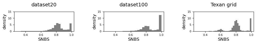
Figure 2: Normalized distributions of the target values (SNBS) in our datasets.

3 Experimental setup to predict SNBS of power grids using GNNs

On both datasets, we train GNNs and baselines on nodal regression tasks. The power grids are represented by the adjacency matrix and a binary feature vector representing sources and sinks. Both are fed into GNNs as input. GNNs are trained to predict SNBS for each node (Figure 1 B). We split the datasets in training, validation and test sets (70:15:15). The validation set is used for the hyperparameter optimization, we report the performance on the test set. To minimize the effect of initializations we use 5 different initializations per model and consider the three best to compute average performances.

We analyze the performance of different GNN models: ArmaNet [37], GCNNet [38], SAGENet [39] and TAGNet [40]. The details of the models based on a hyperparameter study are in Section A.5. To evaluate the performance, we use the coefficient of determination ($R^{2}$-score, see Section A.4).

As baselines we use linear regression and two differently sized MLPs: MLP1 and MLP2. The inputs for MLP and the regression are based on network measures according to Schultz et al. [11]. Details regarding the MLPs and network measures are in Section A.7. Furthermore, we use the best GNN from [32] as additional baseline and call this model Ar-bench.

4 Results of predicting dynamic stability

GNNs accurately predict SNBS

GNN models are remarkably successful at predicting the nonlinear target SNBS, both for dataset2: $R^{2}>82\%$ and for dataset100: $R^{2}>88\%$, see the first two columns in Table 1. Modalities in the data are well captured (left panels in Figure 3). Both MLPs outperform previous work (Ar-bench), but do not achieve the performance of the newly introduced GNNs.

Table 1: Results of predicting SNBS represented by $R^{2}$ score in %. Each column represents a different setup, e.g. for tr20ev100 models are trained on dataset20 and evaluated on dataset100.

model	tr20ev20	tr100ev100	tr20ev100	tr20evTexas	tr100evTexas
Ar-bench	51.20 $\pm$ 2.762	60.24 $\pm$ 0.758	37.87 $\pm$ 2.724	40.34 $\pm$ 2.833	56.86 $\pm$ 1.444
ArmaNet	80.17 $\pm$ 1.226	87.50 $\pm$ 0.081	68.11 $\pm$ 1.933	57.09 $\pm$ 3.079	75.43 $\pm$ 0.635
GCNNet	71.18 $\pm$ 0.137	75.25 $\pm$ 0.151	58.23 $\pm$ 0.059	-5.29 $\pm$ 3.688	65.65 $\pm$ 0.114
SAGENet	65.51 $\pm$ 0.253	75.66 $\pm$ 0.138	51.27 $\pm$ 0.298	32.63 $\pm$ 0.515	53.14 $\pm$ 2.118
TAGNet	83.19 $\pm$ 0.080	88.14 $\pm$ 0.081	67.00 $\pm$ 0.293	56.05 $\pm$ 3.530	82.50 $\pm$ 0.438
linreg	41.75	36.29	5.98	-11.39	-22.62
MLP1	58.47 $\pm$ 0.149	63.59 $\pm$ 0.051	28.49 $\pm$ 1.493	-34.52 $\pm$ 17.93	19.79 $\pm$ 8.659
MLP2	58.20 $\pm$ 0.042	65.52 $\pm$ 0.038	19.65 $\pm$ 2.109	5.81 $\pm$10.58	58.46 $\pm$ 0.370

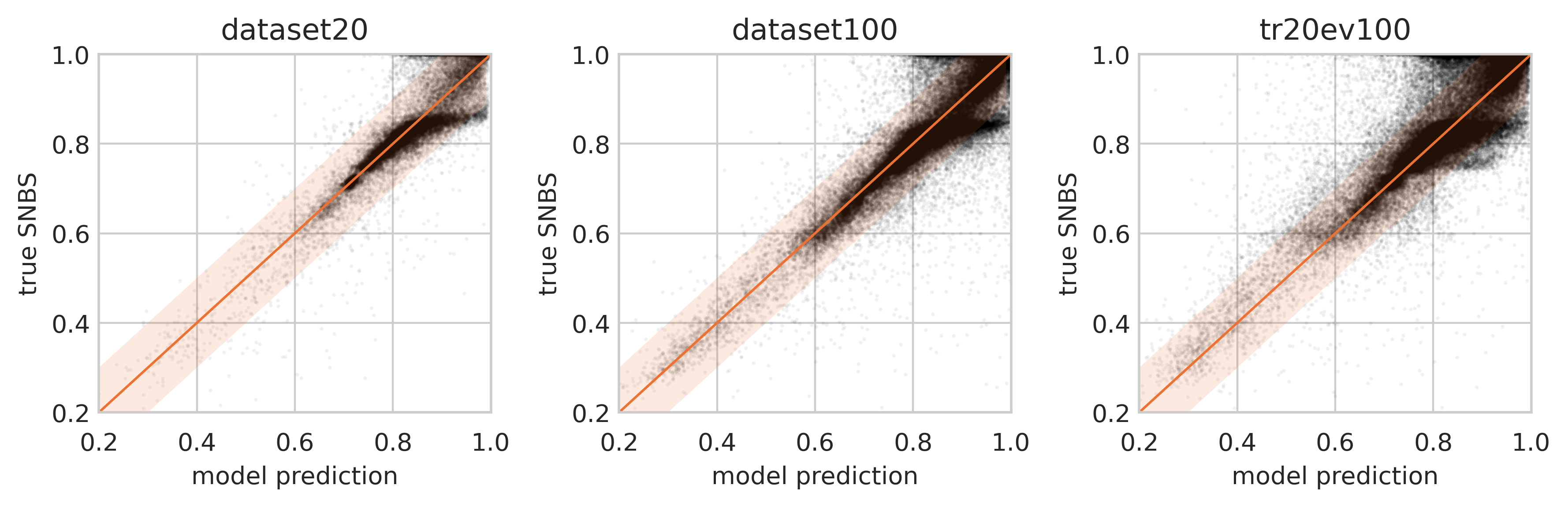
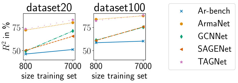
Figure 3: Left panels: Scatterplot of model prediction and true SNBS values of ArmaNet, the diagonal represents a perfect model ($R^{2}=1$), the banded region indicates prediction errors $\leq 0.1$. Right panels: Influence of size of training data on performance.

GNNs perform well at out-of-distrubtion tasks

Using GNNs for SNBS prediction becomes feasible, if they can be trained on relatively simple datasets and still perform well on large, complex grids. Therefore, we define three out-of-distribution tasks: Train on small grids and evaluate on medium-sized grids (tr20ev100), train on small grids and evaluate on the real-sized, synthetic Texan grid (tr20evTexas), and finally train on medium-sized grids and evaluate on the Texan grid (tr100evTexas). The results are shown in Table 1. For the tr20ev100-task all GNNs generalize well and are able to predict SNBS with up to $R^{2}>66\%$. For tr20evTexas the performance is generally worse, with only ARMANet and TAGNet giving somewhat reliable predictions at up to $R^{2}>62\%$. This loss of performance is probably due to the large differences in grid sizes. Most remarkably for the tr100evTexas tasks, all GNN models perform well (except GCN, see Section A.9), with TAGNet reaching an $R^{2}$ of almost $85\%$. The performance of our models is significantly better when trained on the medium-sized grids, indicating that their topological structure is rich enough to allow for generalization to larger grids. This may be the key for real world applications. Importantly, the generalization capabilities of the new GNN models are much better than the baselines using MLP or linear regression.

Training on more data increases the performance of all models

Lastly, we evaluate the benefit of more training data. Our experiments (Figure 3 right) show a clear benefit of more training data as compared to [32], across both grid sizes and all architectures, with differences of up to $\approx 20\%$ in $R^{2}$. We use the new test set for the comparison of all models. Additional results are given in Section A.10.

5 Conclusion and Outlook

This work establishes that GNNs of appropriate size and with enough training data are able to predict probabilistic dynamic stability of models of future power grids with high accuracy. To that end, we provide new datasets 10 times larger than previously published. GNNs trained on the new datasets are able to generalize from small to medium-sized training grids and to real-world sized test grids, promising significant reductions in the simulation time required for grid stability assessment. The datasets and the code to reproduce the results are published on Zenodo and GitHub, see Section A.1. The access enables the community to develop new methods to analyze future renewable power grids.

Acknowledgements

All authors gratefully acknowledge the European Regional Development Fund (ERDF), the German Federal Ministry of Education and Research, and the Land Brandenburg for supporting this project by providing resources on the high-performance computer system at the Potsdam Institute for Climate Impact Research. Michael Lindner greatly acknowledges support by the Berlin International Graduate School in Model and Simulation (BIMoS) and by his doctoral supervisor Eckehard Schöll. Christian Nauck would like to thank the German Federal Environmental Foundation (DBU) for funding his PhD scholarship and Professor Raisch from Technical University Berlin for supervising his PhD. Special thanks go to Julian Stürmer and his supervisors Mehrnaz Anvari and Anton Plietzsch for their assistance with the Texan power grid model.

Appendix A Appendix

This section includes additional information to reproduce the results and also additional results that are not already shown in the main section. We start by providing information on the availability of the data and the used software, followed by details on the evaluation and hyperparameter study and detailed training information for the presented results. Afterwards more results are shown. We also provide details regarding the availability of the datasets and lastly the prediction of SNBS using hand-crafted features, that are considered the baselines in the paper.

A.1 Availability of the datasets

The new datasets and full code for the training, evaluation and generation the figures is published on Zenodo (https://zenodo.org/record/7357903) and GitHub https://github.com/PIK-ICoNe/dynamic_stability_gnn_neurips_climate_workshop.git. It is licensed under CC-BY 4.0 to enable the community to contribute to this challenge.

A.2 Software for generating the datasets

Julia is used for the simulations [41] and the dynamic simulations rely on the package DifferentialEquations.jl [42]. For simulating more realistic power grids in future work we recommend the additional use of NetworkDynamics.jl [43] and PowerDynamics.jl [44].

A.3 Software for training

The training is implemented in Pytorch [45]. For the graph handling and graph convolutional layers we rely on the additional library PyTorch Geometric [46]. We use the SGD-optimizer and as loss function we use the mean squared error . Furthermore ray [47] is used for parallelizing the hyperparameter study.

A.4 Coefficient of determination

To evaluate the performance, the coefficient of determination ($R^{2}$-score) is used and computed by $R^{2}=1-\frac{mse(y,t)}{mse(t_{mean},t)}$, where $mse$ denotes the mean squared error, $y$ the output of the model, $t$ the target value and $t_{mean}$ the mean of all considered targets of the test dataset. $R^{2}$ captures the mean square error relative to a null model that predicts the mean of the test-dataset for all points. The $R^{2}$-score is used to measure the portion of explained variance in a dataset. By design, a model that predicts the mean of SNBS per grids has $R^{2}=0$.

A.5 Hyperparameter optimization

We conduct hyperparameter studies to optimize the model structure regarding number of layers, number of channels and layer-specific parameters using dataset20. The resulting models have the following properties: ArmaNet has 3 layers and 189,048 parameters. GCNNet has 7 layers and 523,020 parameters. SAGENet has 8 layers and 728,869 parameters. TAGNet has 13 layers and 415,320 parameters. Afterwards we optimize learning rate, batch size and scheduler of the best models for dataset20 and dataset100 separately.

We conduct hyperparameter studies in two steps. First, we optimize model properties such as the number of layers and channels as well as layer-specific parameters e.g. the number of stacks and internal layers in case of ArmaNets. For this optimization we use dataset20 and the SNBS task only. For all models we investigated the influence of different numbers of layers and the numbers of channel between multiple layers. We limit the model size to just above four million parameters, so we did not investigate the full presented space, but limited for example the number of channels when adding more layers.

Afterwards we optimize the learning rate, batch size and scheduler of the best models for dataset20 and dataset100. Hence, our models are not optimized to perform well at the out-of distribution task. As GNN baseline, we use the best model from [32] referred to as Ar-bench, which is a GNN model consisting of 1,050 parameters and based on 2 Arma-layers. The only adjustment to that model is the removal of the fully connected layer after the second Arma-Convolution and before applying the Sigmoid-layer, which improves the training.

A.6 Details of the training of the benchmark models

To reproduce the obtained results, more information regarding the training is provided in this section. Detailed information on the training as well as the computation time is shown in Table 2. In case of dataset20, a scheduler is not applied, in case of dataset100, schedulers are used for Ar-bench (stepLR), GCNNet (ReduceLROnPlateau). The default validation and test set batch size is 150. The validation and test batchsize for Ar-bench and ArmaNet3 is 500 in case of dataset20 and 100 for dataset100. The number of trained epochs differs, because the training is terminated in case of significant overfitting. Furthermore, different batch sizes have significant impact on the simulation time. Most of the training success occurs within the first 100 epochs, afterwards the improvements are relatively small.

Table 2: Properties of training models and regarding the training time, we train 5 seeds in parallel using one nVidia V100.

name	number of epochs		training time		train batch size		learning rate
dataset	20	100	20 (hours)	100 (days)	20	100	20	100
Ar-bench	1,000	800	26	4	200	12	0.914	.300
ArmaNet	1,500	1,000	46	6	228	27	3.00	3.00
GCNNet	1,000	1000	29	5	19	79	.307	.286
SAGENet	300	1000	9	5	19	16	1.10	1.23
TAGNet	400	800	11	4	52	52	0.193	.483

A.7 Prediction of SNBS using hand-crafted features

Schultz et al. [11] predict SNBS based on a regression setup using several hand-crafted features. We use a similar setup to compare this approach to the application of GNNs. Based on the work by Schultz et al. [11], we set up a regression task using the following features: degree, average-neigbor-degree, clustering-coefficient, current-flow-betweenness-centrality and closeness-centrality, as well as the nodal feature $P$. For the regression we use the same train and test split.

Training details of MLP

The following hyperparmeters are used: MLP1 has one hidden layer with 35 units per hidden layer, resulting in 1,541 parameters and MLP2 has 6 hidden layers and 500 hidden units per layer resulting in 1,507,001 parameters. We conducted hyperparameter studies to optimize the batch sizes and learning rates, see Table 3.

Table 3: Hyperparameters for the MLPs

model	dataset	learning rate	training batch size
MLP1	dataset20	1.508125539637087	1968
MLP2	dataset20	1.7739583949852091	3367
MLP1	dataset100	1.9519814999342289	303
MLP2	dataset100	0.9978855874564166	3768

A.8 Further Details on power grid generation of the Texan power grid

To take a further step towards real-world applications, we evaluate the performance of our GNN models by analyzing the dynamic stability of a real-sized synthetic model of power grids based on the Texan power grid topology. Real power grid data are not available due to security reasons and calculating an entire SNBS assessment of the fully parameterized synthetic model by [48] appears not to be feasible due to the computational effort [3]. The synthetic grid of Texas is generated using the methods shown in [36]. The Texan power grid model consists of 1,910 nodes after removing 90 nodes that are not relevant for the dispatching. However, that is already a large number and makes the simulations very expensive. the simulation of that grid takes 127,000 CPU hours. Computing less perturbations results in an increased standard error of our estimates of $\pm 0.031$. We use the same modelling approach by arbitrarily modeling nodes as consumers or producers using the $2^{nd}$-order Kuramoto model.

A.9 Poor performance of GCN when applying to the Texan power grid

The GCN model trained on dataset20 is not able to predict the dynamic stability for the Texan power grid. To understand this behaviour, we compare GCNNet and ArmaNet model at the transfer learning task from dataset20 and dataset100 to predict SNBS of the Texan power grid. The scatter plots are shown in Figure 4. We can clearly see that the model is not able to predict lower values of SNBS correctly. The limited output of the GCNNet results in a bad performance in case of the distribution of the Texan power grid that has three modes. As a consequence a model that predicts the mean of the distribution would achieve better performance. Furthermore, we provide the scatter plots of the GCNNet for the three tasks dataset20, dataset100 and tr20ev100 in Figure 5, that can be compared to Figure 3.

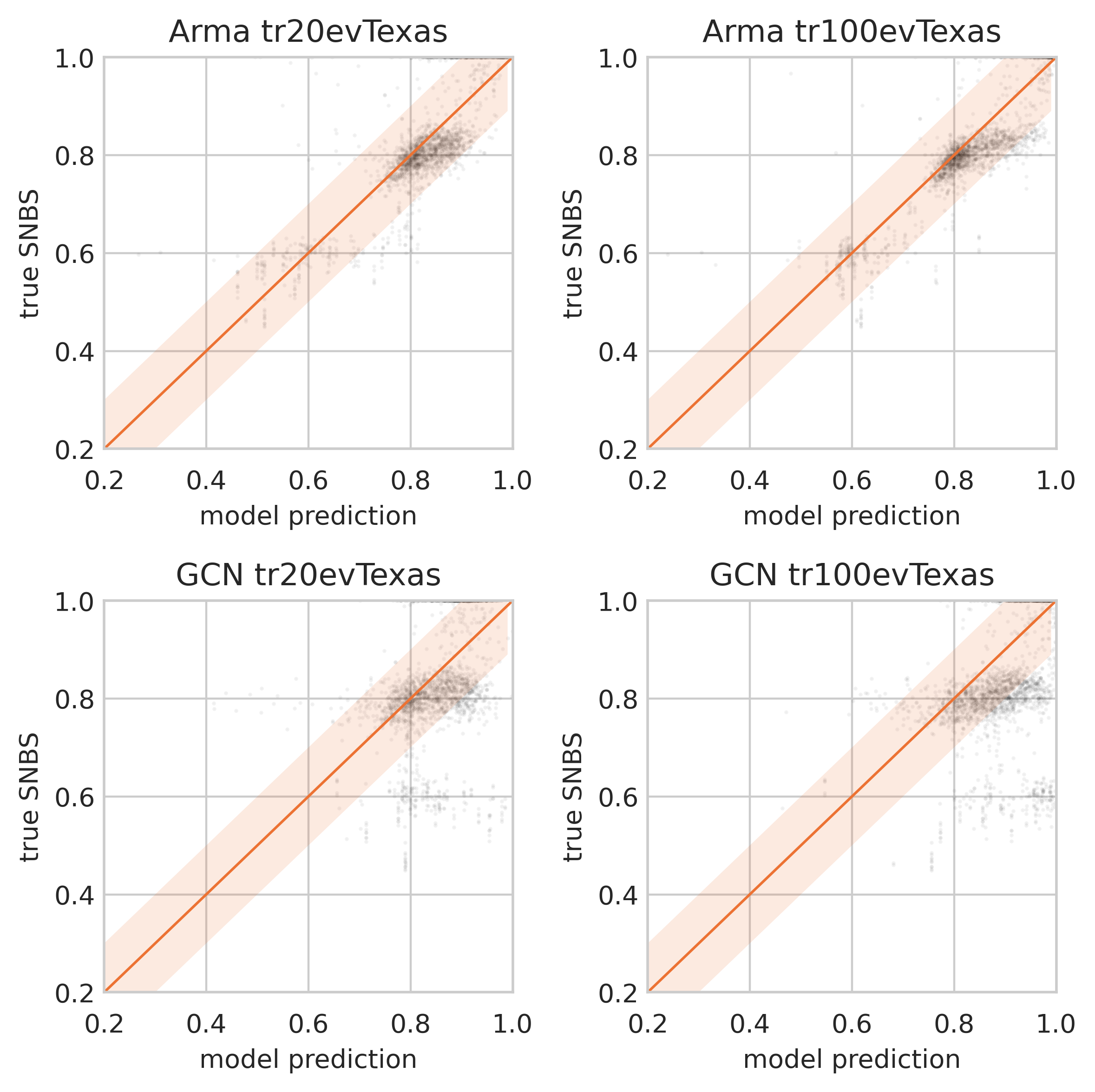
Figure 4: SNBS over predicted output of the Arma and GCN models for the transfer learning task to predict SNBS of the Texan power grid. The diagonal represents a perfect model ($R^{2}=1$), the band indicates the region for accurate predictions based on a tolerance interval of .1 . To account for the small number of nodes, a lower transparency is used in comparison to Figures 3 and 5

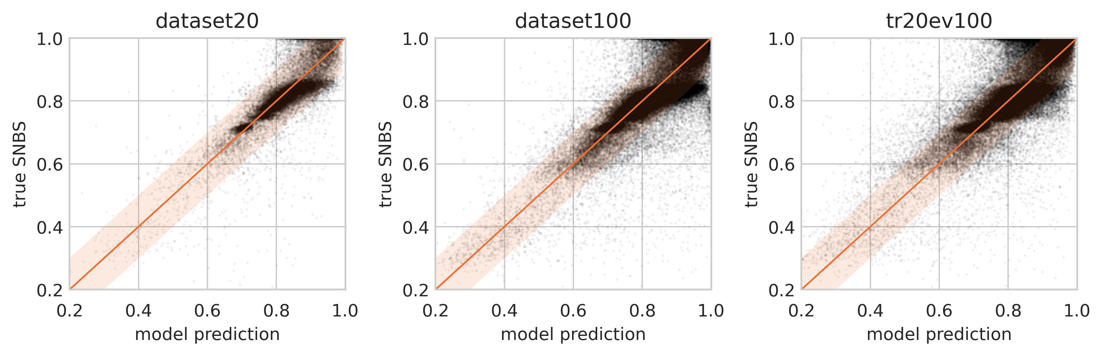
Figure 5: SNBS over predicted output of the GCNNet model for dataset20, dataset100 and trained on dataset20, but evaluated on dataset100. The diagonal represents a perfect model ($R^{2}=1$), the band indicates the region for for accurate predictions based on a threshold of .1

A.10 Detailed results of training on a smaller dataset

To investigate the influence of available training data and to connect with previous work, we train all models on only 800 grids, from [32]. The results are shown in Table 4.

Table 4: Performance after training on smaller training set. All models are trained on the same 800 grids as in [32], but evaluated on the newly introduced test set. The results are represented by $R^{2}$ score in %.

model	dataset20	dataset100	tr20ev100
Ar-bench	46.38 $\pm$ 2.355	58.55 $\pm$ 1.918	31.75 $\pm$ 1.204
ArmaNet	72.20 $\pm$ 1.168	83.70 $\pm$ 0.220	54.12 $\pm$ 3.187
GCNNet	49.48 $\pm$ 0.247	61.26 $\pm$ 1.158	39.59 $\pm$ 0.285
SAGENet	50.26 $\pm$ 0.450	60.94 $\pm$ 0.167	38.93 $\pm$ 0.902
TAGNet	73.30 $\pm$ 0.304	82.21 $\pm$ 0.143	61.47 $\pm$ 0.462

References

- [1] C.B. Field, V. Barros, T.F. Stocker, D. Qin, D.J. Dokken, K.L. Ebi, M.D. Mastrandrea, K.J. Mach, G.-K. Plattner, S.K. Allen, M. Tignor, and P.M. Midgley. Managing the Risks of Extreme Events and Disasters to Advance Climate Change Adaptation. A Special Report of Working Groups I and II of the Intergovernmental Panel on Climate Chan, 2012.
- [2] Hans-Otto Pörtner, D.C. Roberts, M. Tignor, E.S. Poloczanska, K. Mintenbeck, A. Alegría, M. Craig, S. Langdorf, S. Löschke, V. Möller, A. Okem, and B. Rama. IPCC, 2022: Climate Change 2022: Impacts, Adaptation, and Vulnerability. Contribution of Working Group II to the Sixth Assessment Report of the Intergovernmental Panel on Climate Change, 2022.
- [3] Sebastian Liemann, Lia Strenge, Paul Schultz, Holm Hinners, Johannis Porst, Marcel Sarstedt, and Frank Hellmann. Probabilistic Stability Assessment for Active Distribution Grids. In 2021 IEEE Madrid PowerTech, pages 1–6, June 2021.
- [4] Charles D. Brummitt, Paul D. H. Hines, Ian Dobson, Cristopher Moore, and Raissa M. D’Souza. Transdisciplinary electric power grid science. Proceedings of the National Academy of Sciences, 110(30):12159–12159, July 2013. Publisher: Proceedings of the National Academy of Sciences.
- [5] Martin Rohden, Andreas Sorge, Marc Timme, and Dirk Witthaut. Self-Organized Synchronization in Decentralized Power Grids. Physical Review Letters, 109(6):064101, August 2012. Publisher: American Physical Society.
- [6] Adilson E. Motter, Seth A. Myers, Marian Anghel, and Takashi Nishikawa. Spontaneous synchrony in power-grid networks. Nature Physics, 9(3):191–197, March 2013. Number: 3 Publisher: Nature Publishing Group.
- [7] Florian Dörfler, Michael Chertkov, and Francesco Bullo. Synchronization in complex oscillator networks and smart grids. Proceedings of the National Academy of Sciences of the United States of America, 2013.
- [8] Dirk Witthaut, Frank Hellmann, Jürgen Kurths, Stefan Kettemann, Hildegard Meyer-Ortmanns, and Marc Timme. Collective nonlinear dynamics and self-organization in decentralized power grids. Reviews of Modern Physics, 94(1):015005, February 2022. Publisher: American Physical Society.
- [9] Barbara Borkowska. Probabilistic Load Flow. IEEE Transactions on Power Apparatus and Systems, PAS-93(3):752–759, May 1974. Conference Name: IEEE Transactions on Power Apparatus and Systems.
- [10] Peter J. Menck, Jobst Heitzig, Jürgen Kurths, and Hans Joachim Schellnhuber. How dead ends undermine power grid stability. Nature Communications, 5(1):3969, June 2014. Number: 1 Publisher: Nature Publishing Group.
- [11] Paul Schultz, Jobst Heitzig, and Jürgen Kurths. Detours around basin stability in power networks. New Journal of Physics, 16(12):125001, December 2014.
- [12] J. Nitzbon, P. Schultz, J. Heitzig, J. Kurths, and F. Hellmann. Deciphering the imprint of topology on nonlinear dynamical network stability. New Journal of Physics, 19(3):033029, March 2017. Publisher: IOP Publishing.
- [13] Frank Hellmann, Paul Schultz, Patrycja Jaros, Roman Levchenko, Tomasz Kapitaniak, Jürgen Kurths, and Yuri Maistrenko. Network-induced multistability through lossy coupling and exotic solitary states. Nature Communications, 11(1):592, January 2020. Number: 1 Publisher: Nature Publishing Group.
- [14] Zhao Liu and Ziang Zhang. Quantifying transient stability of generators by basin stability and Kuramoto-like models. In 2017 North American Power Symposium (NAPS), pages 1–6, September 2017.
- [15] Zhao Liu, Xi He, Zhenhuan Ding, and Ziang Zhang. A Basin Stability Based Metric for Ranking the Transient Stability of Generators. IEEE Transactions on Industrial Informatics, 15(3):1450–1459, March 2019. Conference Name: IEEE Transactions on Industrial Informatics.
- [16] Dirk Witthaut and Marc Timme. Braess’s paradox in oscillator networks, desynchronization and power outage. New Journal of Physics, 2012.
- [17] Michael M. Bronstein, Joan Bruna, Taco Cohen, and Petar Veličković. Geometric Deep Learning: Grids, Groups, Graphs, Geodesics, and Gauges. arXiv:2104.13478 [cs, stat], May 2021. arXiv: 2104.13478.
- [18] William L. Hamilton. Graph Representation Learning. Synthesis Lectures on Artificial Intelligence and Machine Learning, 14(3):1–159, September 2020.
- [19] Balthazar Donon, Benjamin Donnot, Isabelle Guyon, and Antoine Marot. Graph Neural Solver for Power Systems. In Proceedings of the International Joint Conference on Neural Networks, volume 2019-July. Institute of Electrical and Electronics Engineers Inc., July 2019.
- [20] Cheolmin Kim, Kibaek Kim, Prasanna Balaprakash, and Mihai Anitescu. Graph Convolutional Neural Networks for Optimal Load Shedding under Line Contingency. In 2019 IEEE Power Energy Society General Meeting (PESGM), pages 1–5, August 2019. ISSN: 1944-9933.
- [21] Valentin Bolz, Johannes Rueß, and Andreas Zell. Power Flow Approximation Based on Graph Convolutional Networks. In 2019 18th IEEE International Conference On Machine Learning And Applications (ICMLA), pages 1679–1686, December 2019.
- [22] Nicolas Retiére, Dinh Truc Ha, and Jean-Guy Caputo. Spectral Graph Analysis of the Geometry of Power Flows in Transmission Networks. IEEE Systems Journal, 14(2):2736–2747, June 2020. Conference Name: IEEE Systems Journal.
- [23] Dawei Wang, Kedi Zheng, Qixin Chen, Gang Luo, and Xuan Zhang. Probabilistic Power Flow Solution with Graph Convolutional Network. In 2020 IEEE PES Innovative Smart Grid Technologies Europe (ISGT-Europe), pages 650–654, October 2020.
- [24] Damian Owerko, Fernando Gama, and Alejandro Ribeiro. Optimal Power Flow Using Graph Neural Networks. In ICASSP 2020 - 2020 IEEE International Conference on Acoustics, Speech and Signal Processing (ICASSP), pages 5930–5934, May 2020. ISSN: 2379-190X.
- [25] Fernando Gama, Ekaterina Tolstaya, and Alejandro Ribeiro. Graph Neural Networks for Decentralized Controllers. March 2020. _eprint: 2003.10280.
- [26] George S. Misyris, Andreas Venzke, and Spyros Chatzivasileiadis. Physics-Informed Neural Networks for Power Systems. In 2020 IEEE Power Energy Society General Meeting (PESGM), pages 1–5, August 2020. ISSN: 1944-9933.
- [27] Yuxiao Liu, Ning Zhang, Dan Wu, Audun Botterud, Rui Yao, and Chongqing Kang. Searching for Critical Power System Cascading Failures with Graph Convolutional Network. IEEE Transactions on Control of Network Systems, pages 1–1, 2021. Conference Name: IEEE Transactions on Control of Network Systems.
- [28] Brian Bush, Yuzhou Chen, Dorcas Ofori-Boateng, and Yulia R. Gel. Topological Machine Learning Methods for Power System Responses to Contingencies. Proceedings of the AAAI Conference on Artificial Intelligence, 35(17):15262–15269, May 2021. Number: 17.
- [29] Yuxiao Liu, Ning Zhang, Dan Wu, Audun Botterud, Rui Yao, and Chongqing Kang. Guiding Cascading Failure Search with Interpretable Graph Convolutional Network, January 2020. arXiv:2001.11553 [cs, eess].
- [30] Bukyoung Jhun, Hoyun Choi, Yongsun Lee, Jongshin Lee, Cook Hyun Kim, and B. Kahng. Prediction and mitigation of nonlocal cascading failures using graph neural networks, July 2022. arXiv:2208.00133 [physics].
- [31] Yin Yu, Xinyuan Jiang, Daning Huang, and Yan Li. PIDGeuN: Graph Neural Network-Enabled Transient Dynamics Prediction of Networked Microgrids Through Full-Field Measurement. arXiv:2204.08557 [cs, eess], April 2022. arXiv: 2204.08557.
- [32] Christian Nauck, Michael Lindner, Konstantin Schürholt, Haoming Zhang, Paul Schultz, Jürgen Kurths, Ingrid Isenhardt, and Frank Hellmann. Predicting basin stability of power grids using graph neural networks. New Journal of Physics, 2022.
- [33] Yoshiki Kuramoto. Self-entrainment of a population of coupled non-linear oscillators. Mathematical Problems in Theoretical Physics, 39:420–422, January 1975. ADS Bibcode: 1975LNP….39..420K.
- [34] A.R. Bergen and D.J. Hill. A Structure Preserving Model for Power System Stability Analysis. IEEE Transactions on Power Apparatus and Systems, PAS-100(1):25–35, January 1981. Conference Name: IEEE Transactions on Power Apparatus and Systems.
- [35] Peter J. Menck, Jobst Heitzig, Norbert Marwan, and Jürgen Kurths. How basin stability complements the linear-stability paradigm. Nature Physics, 9(2):89–92, February 2013. Number: 2 Publisher: Nature Publishing Group.
- [36] Adam B. Birchfield, Ti Xu, Kathleen M. Gegner, Komal S. Shetye, and Thomas J. Overbye. Grid Structural Characteristics as Validation Criteria for Synthetic Networks. IEEE Transactions on Power Systems, 32(4):3258–3265, July 2017. Conference Name: IEEE Transactions on Power Systems.
- [37] Filippo Maria Bianchi, Daniele Grattarola, Lorenzo Livi, and Cesare Alippi. Graph Neural Networks with Convolutional ARMA Filters. IEEE Transactions on Pattern Analysis and Machine Intelligence, pages 1–1, 2021. Conference Name: IEEE Transactions on Pattern Analysis and Machine Intelligence.
- [38] Thomas N. Kipf and Max Welling. Semi-Supervised Classification with Graph Convolutional Networks. arXiv:1609.02907 [cs, stat], February 2017. arXiv: 1609.02907.
- [39] William L. Hamilton, Rex Ying, and Jure Leskovec. Inductive representation learning on large graphs. In Advances in Neural Information Processing Systems, 2017. ISSN: 10495258 _eprint: 1706.02216.
- [40] Jian Du, Shanghang Zhang, Guanhang Wu, Jose M. F. Moura, and Soummya Kar. Topology Adaptive Graph Convolutional Networks. October 2017. _eprint: 1710.10370.
- [41] Jeff Bezanson, Alan Edelman, Stefan Karpinski, and Viral B. Shah. Julia: A fresh approach to numerical computing. SIAM Review, 2017. _eprint: 1411.1607.
- [42] Christopher Rackauckas and Qing Nie. DifferentialEquations.jl – A Performant and Feature-Rich Ecosystem for Solving Differential Equations in Julia. Journal of Open Research Software, 5(1):15, May 2017. Number: 1 Publisher: Ubiquity Press.
- [43] Michael Lindner, Lucas Lincoln, Fenja Drauschke, Julia M. Koulen, Hans Würfel, Anton Plietzsch, and Frank Hellmann. NetworkDynamics.jl—Composing and simulating complex networks in Julia. Chaos: An Interdisciplinary Journal of Nonlinear Science, 31(6):063133, June 2021. Publisher: American Institute of Physics.
- [44] Anton Plietzsch, Raphael Kogler, Sabine Auer, Julia Merino, Asier Gil-de Muro, Jan Liße, Christina Vogel, and Frank Hellmann. PowerDynamics.jl – An experimentally validated open-source package for the dynamical analysis of power grids. arXiv:2101.02103 [cs, eess], January 2021. arXiv: 2101.02103.
- [45] Adam Paszke, Sam Gross, Francisco Massa, Adam Lerer, James Bradbury, Gregory Chanan, Trevor Killeen, Zeming Lin, Natalia Gimelshein, Luca Antiga, Alban Desmaison, Andreas Kopf, Edward Yang, Zachary DeVito, Martin Raison, Alykhan Tejani, Sasank Chilamkurthy, Benoit Steiner, Lu Fang, Junjie Bai, and Soumith Chintala. PyTorch: An Imperative Style, High-Performance Deep Learning Library. In H. Wallach, H. Larochelle, A. Beygelzimer, F. d\textquotesingle Alché-Buc, E. Fox, and R. Garnett, editors, Advances in Neural Information Processing Systems 32, pages 8024–8035. Curran Associates, Inc., 2019.
- [46] Matthias Fey and Jan E Lenssen. FAST GRAPH REPRESENTATION LEARNING WITH PYTORCH GEOMETRIC. page 9, 2019.
- [47] Philipp Moritz, Robert Nishihara, Stephanie Wang, Alexey Tumanov, Richard Liaw, Eric Liang, Melih Elibol, Zongheng Yang, William Paul, Michael I. Jordan, and Ion Stoica. Ray: A Distributed Framework for Emerging AI Applications. arXiv:1712.05889 [cs, stat], September 2018. arXiv: 1712.05889.
- [48] Adam Birchfield. ACTIVSg2000: 2000-bus synthetic grid on footprint of Texas, visited on Nov. 1, 2021.