Landau Theory of Causal Dynamical Triangulations

Abstract

Understanding the continuum limit of a theory of discrete random geometries is a beautiful but difficult challenge. In this optic, we review here the insights that can be obtained for Causal Dynamical Triangulations (CDT) by employing the Landau approach to critical phenomena. In particular, concentrating on the cases of two and three dimensions, we will make the case that the configuration of the volume of spatial slices effectively plays the role of an order parameter, helping us to understand the phase structure of CDT. Moreover, consistency with numerical simulations of CDT provides hints that the effective field theory of the model lives in the space of theories invariant under foliation-preserving diffeomorphisms. Among such theories, Hořava-Lifshitz gravity has the special status of being a perturbatively renormalizable theory, while General Relativity sits in a subspace with enhanced symmetry. In order to reach either of them, one would likely need to fine tune some of the parameters in the CDT action, or additional ones from some generalization thereof.

Note: This is a contribution to the Handbook of Quantum Gravity which is expected to be published in 2023. It will appear as a chapter in the section dedicated to Causal Dynamical Triangulations.

1 Introduction

Lattice regularization is a common approach to taming in a nonperturbative way the ultraviolet divergences of a quantum field theory. For many quantum field theories it is relatively straightforward to formulate a corresponding lattice field theory, but showing that a nontrivial continuum limit can be obtained is generally very difficult. The standard physical picture, based on the Wilsonian renormalization group, is that such a limit should exist if the lattice model has a second-order phase transition that requires the tuning of the interaction coupling in order to be reached. In such a scenario, one would construct the continuum limit as a scaling limit in which the coupling is tuned to the phase transition in a coordinated way with the tuning of the lattice spacing to zero. Lacking an exact solution for the given model, such a scaling limit is a challenging task, especially when the universality class of the phase transition is described by an interacting theory. Luckily, even simple calculations and approximations can often help in establishing a correct physical picture. In particular, the Landau theory of critical phenomena provides very often a qualitatively (if not quantitatively) correct description of the phase transitions of a model.

In gravity, even the first step of formulating a lattice theory is nontrivial. Indeed, in general relativity the gravitational force is described in terms of the geometry of spacetime, whose dynamics is governed by background independent laws, so we should not rely on a fixed lattice background. One proposal to construct a candidate lattice theory of Euclidean quantum gravity took shape in the 1980’s in the context of noncritical bosonic string theory, and it is commonly known as dynamical triangulations (DT) Ambjorn:1997di . It is based on Regge’s coordinate-free approach to discrete gravity Regge:1961px , in which continuous manifolds are replaced by piecewise flat manifolds (triangulations and their higher-dimensional generalizations, simplicial manifolds). However, unlike in Regge calculus, in DT one is prescribed to sum over all possible triangulations, with all edge-lengths fixed to the same value $a$, thus making DT also intrinsically background independent, in the sense that there is no fixed structure at all and no identifiable points. Originally DT was constructed for two-dimensional quantum gravity David:1984tx ; Ambjorn:1985az ; Kazakov:1985ea , in which case it is related to matrix models DiFrancesco:1993nw , and it had an exciting success in reproducing continuum results in the case of conformal charge $c<1$, thus proving that this way of discretizing the functional integral over geometries makes sense. Later, it was generalized to three and four dimensions, where however the results were more disappointing: no second-order phase transition could be found deBakker:1996zx ; Bialas:1996wu . Moreover, the two phases of the model, separated by a first-order transition, were characterized by very degenerate geometries that did not approach a classical limit at large scales Ambjorn:1995dj .

The state of affairs was significantly improved with the introduction of the model of causal dynamical triangulations (CDT) by Ambjorn and Loll (initially in two dimensions Ambjorn:1998xu , and later in three and four dimensions, together with Jurkiewicz Ambjorn:2001cv ; Ambjorn:2005qt ). CDT modifies DT only by the requirement that the ensemble of triangulations be restricted with the requirement that each triangulation carries a non-singular foliation, i.e. a clear $(d+1)$-dimensional decomposition with $d$-dimensional slices (or leaves) of fixed topology, subsequent slices being always at fixed distance from each other (see Ambjorn:2001cv for the precise construction, or the two-dimensional example in Fig. 1 for an intuitive understanding). Notice in particular that the foliation induces a natural notion of time as the direction perpendicular to the foliation, and a natural choice of time coordinate $t$, such that all the vertices on a given slice are at the same value of $t$. With such a simple modification, originally motivated by the requirement of having always nonsingular light cones in a Lorentzian version of the model, the main problems of DT seemed to have been solved: a new phase of the model emerged with some classical behavior at large scales Ambjorn:2005qt , separated from another phase by a second-order phase transition Ambjorn:2012ij (see the reviews Ambjorn:2012jv ; Loll:2019rdj for a proper summary of results and a complete list references).

Figure 1: Example of a triangulated portion of spacetime in the two-dimensional CDT model. The flattened picture captures the way triangles are glued together, but does not represent faithfully intrinsic distances, as edge lengths should be all equal.

We should at this stage take a step back, and reflect upon the way phase diagrams are found in these models, which are effectively statistical models of random geometry. As for any statistical model, the standard way to chart a phase diagram is to identify suitable order parameters taking different values in the different phases. Such order parameters should necessarily correspond to expectation values of observables, meaning quantities which are independent of (unobservable) gauge choices. Here one stumbles in the problem of observables in quantum gravity (e.g. Rovelli:1990ph ; Giddings:2005id ): as in any diffeomorphism invariant and background independent approach to quantum gravity, observables in DT are necessarily nonlocal. Luckily, this is not an immediate problem for the phase diagram, as order parameters are often nonlocal (e.g. the average magnetization in the Ising model), at least for the identification of homogenous phases, and indeed the two phases of DT can be distinguished by a global observable: the average linear size of the “universe”. In particular, studying the scaling of it with the total volume of the universe, one can define an effective Hausdorff dimension $d_{H}$ of the averaged universe. It turns out that for topological dimension $d=3$ and $4$, varying the lattice Newton constant, the effective dimension jumps from $d_{H}\sim 2$ (branched polymer phase) to $d_{H}\sim\infty$ (crumpled phase) Ambjorn:1995dj . Phases with the same Hausdorff dimensions were also found in CDT, but in addition a new phase was identified as well, with $d_{H}\sim d$ Ambjorn:2005qt . Clearly, this was a great advance, providing a zeroth order test of classical behavior being possible in these models, but much more is needed in order to reconstruct the possible continuum limit. For the latter, global observables are not very instructive, as for example it is hard to imagine how to construct and interpret an effective action for the Hausdorff dimension.

In CDT, thanks to the foliation, more observables are available, of a slightly more local nature: observables that are local in time but non-local in space. The easiest observable of this type is the volume of spatial slices $N_{d-1}(t)$, simply counting the number of $(d-1)$-simplices in the spatial slice at time $t$. Armed with such observable, one can characterize the different phases of CDT in terms of volume profiles, and even derive an effective action describing the dynamics of the spatial volume Ambjorn:2004pw . The latter will be our main focus in the following.

Given the premises above, a natural question arises: are the foliation and its associated observables compatible with a fully diffeomorphism invariant and background independent continuum limit? Originally, the foliation was thought only as a way of selecting less pathological geometries in a partially gauge-fixed (proper time gauge) version of discrete quantum gravity (see Dasgupta:2001ue for a continuum point of view on this). However, the existence of observables that are local in time raises two problems: first, they would be just a gauge artifact, and should not be true observables of the theory; second, a coarse-grained effective action depending on them would only be compatible with a gauge-fixed general-covariant action for very special values of the couplings. The last point is extremely important, and, phrased differently, means that the most general and natural theory space in which a renormalization group flow of CDT should take place is that of theories invariant under foliation-preserving diffeomorphisms (FPD), and invariance under full (spacetime) diffeomorphisms would only be recovered on a submanifold of theory space. FPD-invariant theories were introduced by Hořava Horava:2008ih ; Horava:2009uw in order to construct a gravitational theory that could be at the same time perturbatively renormalizable and unitary. This is achieved by introducing in the action higher derivatives in space, but not in time, which is possible thanks to the reduced diffeomorphism invariance. Such theories, of which several versions have been introduced and studied (see Wang:2017brl ; Steinwachs:2020jkj for reviews), are commonly known as Hořava-Lifshitz (HL) gravity, as they are the gravitational analog of theories with a Lifshitz critical point. On the other hand, the space of FPD-invariant effective theories is more general and contains in particular also nonrenormalizable ones.

First possible hints of a relation between CDT and HL-type gravity theories were discussed in Horava:2009if ; Benedetti:2009ge ; Ambjorn:2010hu , relying mostly on the presence of a foliation, on a qualitative resemblance between the phase diagram of CDT with the generic Lifshitz phase diagram, and on results concerning the spectral dimension (another useful notion of effective dimension). Other dynamical arguments have subsequently been added Budd:2011zm ; Ambjorn:2013joa ; Benedetti:2014dra ; Benedetti:2016rwo , and a longer list of arguments will be reviewed in Sec. 5, but of course understanding the continuum limit of higher-dimensional background-independent statistical models like CDT is highly nontrivial, and therefore the precise relation is still open, in particular in four dimensions.

In any case, the fact that FPD-invariant effective theories are conceivable theories of dynamical geometry raises the following question: if CDT was describing a partially gauge-fixed but otherwise fully covariant theory, how would we construct a nonperturbative quantization of FPD-invariant theories in the spirit of dynamical triangulations, if not by introducing a foliation as in CDT? Most likely, the answer is that for FPD-invariant theories we should indeed use the same ensemble of triangulations as in CDT, in general with a different action, with more parameters (as for example in Anderson:2011bj ). And if a fully diffeomorphism-invariant continuum limit could ever be reached from such generalized CDT models, this should be found within a subspace of their full theory space, i.e. by a careful fine tuning of the couplings. Could we be so lucky that the standard CDT already sits in such a subspace? This might seem plausible, at least in two and three dimensions, where the CDT action is just a Regge discretization of the Einstein-Hilbert action, with cosmological and Newton constant. Consider the example of a scalar model on a regular lattice. Typically, an anisotropic action will lead to an anisotropic continuum limit, while discrete rotation symmetry will result in full rotation invariance in the continuum limit (see for example Borji:2020snd ). That is, in this case, starting from an action which is a simple discretization of a rotation-invariant action, leads to the expected result, or in other words, the fine tuning is trivial. But rotation invariance is a global symmetry. Things are more complicated for gauge symmetries, as their breaking leads to new degrees of freedom: for example, HL gravity has a new scalar degree of freedom besides the massless spin-2 graviton. It is a well known fact that in the case that the gauge invariance of a quantum field theory is broken by a lattice or by a momentum cutoff, in order to restore it in the continuum limit, and thus recover the desired target theory, one needs a nontrivial fine tuning of all the possible breaking terms in the action, as for example extensively discussed in some lattice approach to chirality Testa:1997ia , or in constructive Magnen:1992wv and functional renormalization group Ellwanger:1994iz ; Gies:2006wv approaches to Yang-Mills theory. It seems reasonable to expect that recovering full diffeomorphism invariance in CDT would require some fine tuning along those lines.

Let us recap the key elements of the discussion above. DT models provide a diffeomorphism invariant and background independent discretization of a quantum theory of dynamical geometry, but unfortunately they do not have a second order phase transition and they are dominated by very degenerate geometries. In order to solve these problems, in CDT one reduces the ensemble of triangulations by introducing a built-in regular foliation. However, the foliation being a sort of background structure, this likely breaks part of the diffeomorphism invariance of the target theory (general relativity), and in order to restore that, one would presumably need to fine tune the model, as well as add new counterterms to the action. The latter part of this summary is so far conjectural, because, due to the complexity of the models, which are mostly studied by Monte Carlo simulations, we cannot rule out in all certainty that the standard CDT action would be a lucky choice leading to a full diffeomorphism invariant theory in the continuum.

We will argue below that in two dimensions it is quite clear that indeed in the continuum limit CDT is described by an FPD-invariant theory, that in three dimensions there is some evidence supporting the same conclusion, and that even in four dimensions there are some indications in the same direction. To that end, we will focus on the effective dynamics of the volume of the spatial slices, which can be seen as an application of Landau theory to CDT. In particular, we will argue that by a deeper study of the effective action governing such observable, one can in principle distinguish between a gauge-fixed general-covariant action and an FPD-invariant one.

The rest of the review, mainly based on the results of Benedetti:2014dra ; Benedetti:2016rwo , is organized as follows. In section 2, we review the main ideas of the Landau theory of critical phenomena, the challenges of applying it to a background independent model, and how instead a Landau free energy is straightforwardly obtained for two-dimensional CDT, in a direct top-down approach. Armed with that, one recognizes in the continuum limit the two-dimensional version of HL gravity. In section 3, we review the setup and numerical results for the dynamics of the spatial volumes in three-dimensional CDT. In section 4, we review a bottom-up proposal (based on numerical data and on the intuitions we tried to motivate in this introduction) for the Landau free energy associated to such spatial volumes, viewed as (time-dependent) order parameter of the model. We also review the numerical simulations of the coarse-grained model based on such Landau free energy, showing that qualitative features of the CDT phase diagram are reproduced. An extremization analysis of the continuum limit of the Landau free energy is reviewed in section 4.3, providing in particular an analytical understanding of the condensation phenomenon observed in the semiclassical phase of CDT, and one more indication that the correct effective action of the model sits in the space of FPD-invariant theories. Lastly, we conclude in section 5 with a short summary, and a discussion of our current understanding of the relation between CDT and HL-like gravity theories.

2 Landau Theory and CDT

The goal of Landau theory (e.g. Goldenfeld:1992qy ) is to provide a theoretical framework for understanding and predicting phase transitions in statistical systems. In this respect, it has represented an important landmark in statistical physics, successfully explaining many phenomena. It is also well-known to have strong limitations, predicting wrong scaling exponents below critical dimensions, and this led to the development of the renormalization group. However, in general Landau theory remains a valid tool for a first analysis, at least at the qualitative level, for example for understanding the structure of the phase diagram of a given model.

The central aspect of Landau theory is that it postulates that phase diagrams can be explained in terms of order parameters, and that these are effectively governed by a coarse-grained free energy functional, known as Landau free energy, which depends parametrically on the coupling constants of the system. The minima of the Landau free energy determine the thermodynamically favored configuration of the order parameters, and different favored configurations correspond to different phases. Typically, there will be a disordered phase, with vanishing order parameters and unbroken symmetries, and one or more ordered phases, with non-vanishing order parameters breaking some or all of the symmetries of the system. Therefore, given a statistical model, it is crucial to identify the order parameters and construct the corresponding Landau free energy.

There are two main approaches for constructing the Landau free energy: a phenomenological (bottom-up) approach, writing it as an expansion in the order parameters, constrained by the symmetries, as in effective field theories; and a top-down approach, deriving the Landau free energy by explicitly coarse-graining the microscopic model. The latter is of course seldomly applicable in practice, but it provides a very instructive way of thinking about the Landau theory, and it is hence worth of being briefly recalled (we essentially follow Goldenfeld:1992qy for this).

Consider a spin system with Hamiltonian $H(\{s\})$, where $\{s\}=\{s_{i}\mid i\in\mathcal{L}\}$ is a configuration of spin variables $s_{i}$ on the $N$ sites of the lattice $\mathcal{L}$. The partition function is

$$Z_{\rm spin}=\sum_{\{s\}}e^{-\beta H(\{s\})}\,.$$ (1)

Next, partition the lattice into blocks $\mathcal{B}_{r}$, labeled by $r$, which can be thought of as a site of the coarse grained lattice $\mathcal{L}^{\prime}$. Each block contains $N(r)$ sites, such that $\sum_{r}N(r)=N$. We define the Landau free energy $L(\{m\})$, where $\{m\}=\{m(r)\mid r\in\mathcal{L}^{\prime}\}$, as the Gibbs free energy for the system, constrained to be in a configuration compatible with a local magnetisation configuration specified by $\{m\}$, i.e.:

$$e^{-L(\{m\})}=\sum_{\{s_{i}\mid i\in\mathcal{L},\,\frac{1}{N(r)}\sum_{j\in\mathcal{B}_{r}}s_{j}=m(r)\}}e^{-\beta H(\{s\})}\,.$$ (2)

From the definitions, it follows straightforwardly that the partition function can be expressed in terms of the Landau free energy as

$$Z_{\rm spin}=\sum_{\{m\}}e^{-L(\{m\})}\,.$$ (3)

It is clear that in this construction, $L(\{m\})$ can also be thought as a Wilsonian effective Hamiltonian. This is in particular the case because the local magnetisation $\{m\}$ is a similar (albeit coarse grained) type of variable as the original spin variables $\{s\}$, in the sense that we went from some spin variables to some other spin variables (perhaps with a different set of values, due to the averaging). The idea is however more general, and depending on the model and the relevant order parameter, one can define different coarse-graining procedures and end up with very different variables.

Landau theory and quantum gravity. Applying a similar construction to quantum gravity is of course marred with difficulties, in particular concerning the identification of order parameters, as observables are notoriously problematic in quantum gravity. Diffeomorphism invariance and background independence constrain observables to be non-local quantities, which are not very suitable for reconstructing a local effective action. Moreover, coarse graining presents several practical and conceptual obstacles, due to the absence of a background structure. Nevertheless, inventive approaches to the problem have been devised, with coarse graining procedures introduced for constructing a renormalization group flow in DT Johnston:1994qi ; Thorleifsson:1995ki ; Ambjorn:1996hu ; Renken:1996kf ; Henson:2009fy and in spin foams Markopoulou:2002ja ; Oeckl:2002ia ; Bahr:2012qj ; Dittrich:2013uqe ; Steinhaus:2020lgb . More to the point of interest here, mean field models of DT have also been proposed Renken:1997na ; Bialas:1998ci . The latter involved no coarse graining, they were rather in the spirit of defining approximated Hamiltonians (or actions, in the parlance of Euclidean QG) much like what is done when replacing the Ising model Hamiltonian with one in which spin interacts not just with its neighbour, but with an average of all the other spins (the mean field). Again this procedure, which is straightforward in the Ising case, is not at all obvious in DT, and in fact the mean field models for DT were postulated, rather than derived from the model itself.

Once more, in CDT things are (slightly) different thanks to the foliation. Small-step blocking is still a very clumsy procedure, but we do have a natural partitioning of the lattice into large blocks: the leaves of the foliations. We can therefore define a Landau free energy by summing over all triangulations that on each slice lead to a prescribed value for a nonlocal slice observable. As anticipated, the choice of slice observable on which we will concentrate is the volume of the slice, which is essentially the only one studied so far, but it would be interesting to explore other options. As a way of clarifying this set of ideas, and of introducing the more difficult higher-dimensional cases, we start by analyzing the two-dimensional CDT model in this perspective.

2.1 CDT in a nutshell

The CDT approach exactly parallels the usual lattice field theory with one fundamental difference: the fixed lattice is replaced by an ensemble of random triangulations. This is required by the fact that gravity is a theory of dynamical geometry, with no background spacetime fixed a priori.

More concretely, one defines an ensemble of “triangulations” to work with, a triangulation being defined by a simplicial manifold, i.e. a collection of $d$-dimensional flat simplices (the generalization of triangles and tetrahedra) glued along their $(d-1)$-dimensional faces and such that the neighbourhood of any vertex is homeomorphic to a $d$-dimensional ball. A dynamical triangulation is one in which all the simplices are taken to be equilateral. In the simulations we usually work with dynamical triangulations having a fixed number of $d$-simplices $N$, which we will denote $\mathcal{T}_{N}$. The ensemble of such triangulations $\{\mathcal{T}_{N}\}$ is obtained by gluing the $N$ simplices in all possible ways allowed by the simplicial manifold condition, and respecting a chosen topology. Furthermore, to avoid the sick behaviour that was found in the old models of dynamical triangulations, CDT models have one further restriction on the ensemble: only triangulations with a global time foliation, with respect to which no spatial topology change occurs, are allowed. For more details on the geometrical meaning of this restriction and on its implementation see Ambjorn:2001cv .

Once the ensemble is specified one can construct the partition function (Euclidean version of the path integral) as

$$Z=\sum_{N}\sum_{\mathcal{T}_{N}}\tfrac{1}{C(\mathcal{T}_{N})}\,e^{-S(\mathcal{T}_{N})}\,,$$ (4)

where $S(\mathcal{T}_{N})$ is the bare action, and $C(\mathcal{T}_{N})$ is the order of the automorphism group of $\mathcal{T}_{N}$, a symmetry factor naturally appearing when summing over unlabeled triangulations (e.g. Ambjorn:2012jv ). Since we wish to recover general relativity in the classical limit, it is customary to use as a bare action the Einstein-Hilbert action adapted to a simplicial manifold, which is known as the Regge action. On a dynamical triangulation, the Regge action takes the very simple form

$$S(\mathcal{T}_{N})=\kappa_{d}N-\kappa_{d-2}N_{d-2}\,,$$ (5)

where $\kappa_{d}$ and $\kappa_{d-2}$ are two coupling constants depending on the cosmological and Newton’s constant appearing in the Regge action, and $N_{d-2}$ is the number of $(d-2)$-dimensional subsimplices (also called bones or hinges).

In principle one could use a different action, with more parameters, but at this stage this would only complicate the analysis of the results, and in a minimalist attitude such a generalization of the CDT models is usually postponed till the moment (if ever) at which the model itself will ask for such an extension. For example in $3+1$ dimensions a new parameter has been introduced in the action, without which no physically interesting region would exist in the phase diagram Ambjorn:2005qt . Furthermore, we need to remember that, for fixed topology, only $d/2$ (for $d$ even) or $(d+1)/2$ (for $d$ odd) among the values $\{N_{0},N_{1},...N_{d-1},N_{d}=N\}$ are independent. Hence, for $d=3$ and $d=4$ only two of such variables are independent, and as a consequence, if we want to keep the action linear in $N_{j}$, we only have two coupling constants. The counting changes in CDT because we can distinguish subsimplices whose vertices are all on one slice from those having vertices on two adjacent slices, and additional variables can be introduced in order to keep track of that. However, new topological relations are found too. The counting for CDT was carried out in Ambjorn:2001cv , and one has that for $d=4$ there are 10 variables and 7 constraints, leaving 3 independent variables, a fact that was used in Ambjorn:2005qt to introduce the new parameter. In $d=3$ the situation is instead unchanged with respect to the DT case, as there are 5 constraints for 7 variables, and hence again only 2 independent variables. For this reason it is not possible to introduce in three dimensions the analogue of the new parameter used in four dimensions.

2.2 Balls-in-boxes models

Before continuing our discussion of CDT, it is useful to introduce the so-called balls-in-boxes (BIB) models, as they will play the role of effective models of CDT.

The statistical models known as balls-in-boxes (or zero-range process in the nonequilibrium version) are an interesting and versatile class of models which have been extensively studied in the statistical mechanics literature (see for example Evans-review ). They have also been used as mean field models of DT Bialas:1996eh ; Bialas:1997qs ; Bialas:1998ci , and later, also as effective models for the spatial volume dynamics of CDT in 3+1 dimensions Bogacz:2012sa . We briefly review in this section their definition and some of their relevant properties.

A BIB model is defined as a one-dimensional lattice with $T$ sites (boxes) to each of which is associated an integer number $m_{i}\geq m_{\rm min}\geq 0$ (the number of balls in box $i\in\{1,2,...,T\}$). The total number of balls is fixed to be $M$. The canonical partition function of the statistical model is given as

$$\begin{split}Z_{\rm BIB}(T,M)&=\sum_{m_{1}=m_{\rm min}}^{M}...\sum_{m_{T}=m_{\rm min}}^{M}\delta_{M,\sum_{i}m_{i}}\prod_{i=1}^{T}g(m_{i},m_{i+1})\\ &=\sum_{\{m_{j}\}}e^{-S(\{m_{j}\})}\delta_{M,\sum_{i}m_{i}}\,,\end{split}$$ (6)

with $m_{T+1}=m_{1}$. The last expression highlights the interpretation of such models as discretised one-dimensional path integrals, subjected to the constraint

$$\sum_{i=1}^{T}m_{i}=M\,.$$ (7)

The weight function $g(m,n)$ (or the action $S(\{m_{j}\})$) defines the particular model. In the standard BIB models there is no nearest-neighbour interaction, meaning that $g(m_{i},m_{i+1})=g(m_{i})$; the model above is a generalisation studied in Evans-prl ; Waclaw:2009zz .

Often, in particular for an analytical approach, it is useful to work in the grand canonical ensemble, for which the partition function reads

$$\begin{split}Z_{\rm BIB-gc}(T,z)&=\sum_{M}Z_{\rm BIB}(T,M)\,z^{M}\\ &=\operatorname{Tr}\,\hat{T}^{T}\,,\end{split}$$ (8)

where we introduced the transfer matrix

$$\hat{T}_{m,n}=z^{(m+n)/2}g(m,n)\,.$$ (9)

In the light of this relation, $g(m,n)$ is sometimes referred to as reduced transfer matrix.

One interesting feature of these models is that they can exhibit a condensation phenomenon. In the original BIB models, with $g(m_{i},m_{i+1})=g(m_{i})$, this means that for certain values of the parameters the model enters into a phase dominated by configurations completely localised at one (random) site. The mechanism behind such condensation remains similar in the more general models, but the nearest-neighbour interaction allows the condensate to spread over a region whose width scales with a power of the total volume $M$. As we will see, it is this type of condensation which provides the basis for an explanation of the droplet configuration in CDT based on the much simpler BIB models.

2.3 Landau theory of two-dimensional CDT

In two dimensions, only one of the $N_{k}$ variables is independent, e.g. the number of triangles $N_{2}$. This is clear also from a continuum perspective, as the curvature term is topological, hence at fixed topology the Einstein-Hilbert action reduces to a simple volume term. The two-dimensional CDT model Ambjorn:1998xu at fixed topology has thus only one coupling, the bare cosmological constant, while Newton’s constant plays no role. The corresponding partition function has therefore the interpretation of generating function for the number of triangulations of the type in figure 1 with fixed number of triangles $N$ and some given boundary conditions. Typically one fixes also the number of time slices $T$, which in fact can be seen as a new free variable, appearing thanks to the foliation.

The two-dimensional model of CDT can be solved exactly by various means Ambjorn:1998xu ; DiFrancesco:1999em ; DiFrancesco:2000nn ; DiFrancesco:2001xur , so it would seem pointless to look for a Landau theory. However, the latter appears very naturally in the process of solving the model, and it is therefore a useful example of top-down approach to a Landau free energy in a quantum gravity model. In this case, the partition function for causal triangulations with fixed $N$ and $T$ (denoted ($\mathcal{T}_{N,T}$) can be written as

$$\begin{split}Z_{\rm 2d-CDT}(N,T)&=\sum_{\mathcal{T}_{N,T}}1\\ &=\sum_{l_{1}=1}^{N}...\sum_{l_{T}=1}^{N}\delta_{N_{2},2\sum_{i}l_{i}}\prod_{i=1}^{T}g(l_{i},l_{i+1})\\ &\equiv\sum_{\{l\}}e^{-L(\{l\};N,T)}\,,\end{split}$$ (10)

with $l_{T+1}=l_{1}$ (periodic boundary conditions in the time direction), and

$$g(l_{i},l_{i+1})=\frac{(l_{i}+l_{i+1})!}{l_{i}!\,l_{i+1}!}\,,$$ (11)

counting the number of triangulations of a strip with boundary lengths $l_{i}$ and $l_{i+1}$, with open boundary conditions.

In the second line of (10) we recognize a BIB model (compare to (6)), while in the last line we defined the function $L(\{l\};N,T)$, which we interpret as a Landau free energy. Indeed, comparing to (2) and (3), we see that in the definition of $L(\{l\};N,T)$ we are summing over triangulations with a block constraint, the blocks here being the spatial slices of each triangulation, and the constraint fixing the number of edges in each block.

Notice that the Landau free energy $L(\{l\};N,T)$ contains a global constraint, but we can get rid of it by switching to the grandcanonical ensemble. That is, by summing over $N$ with a Boltzmann weight $e^{-\kappa_{2}N}$, we obtain:

$$L_{\rm gc}(\{l\};T,\kappa_{2})=2\kappa_{2}\sum_{i}l_{i}-\sum_{i}\ln\left(g(l_{i},l_{i+1})\right)\,.$$ (12)

It should be stressed that the second term is a purely entropic contribution, with no lattice coupling constant.

Continuum limit. The model is exactly solvable Ambjorn:1998xu ; DiFrancesco:1999em ; DiFrancesco:2000nn ; DiFrancesco:2001xur , and a continuum limit can be taken on the solution. It is however instructive to see what we can learn by first taking a continuum approximation, and then minimizing the continuum Landau free energy. Using Stirling’s formula one finds that, for large $l_{i}$ and $l_{i+1}$, and small $(l_{i+1}-l_{i})/(l_{i}+l_{i+1})$,

$$g(l_{i},l_{i+1})\sim 2^{l_{i}+l_{i+1}}e^{-\frac{(l_{i+1}-l_{i})^{2}}{l_{i}+l_{i+1}}}\,.$$ (13)

It is easy to take the continuum limit of the exponent in (13), thus obtaining

$$S_{\rm 2d-HL}[\ell]=\int_{-\frac{\tau}{2}}^{\frac{\tau}{2}}dt\,\frac{\dot{\ell}(t)^{2}}{4\ell(t)}\,.$$ (14)

Such action can be interpreted as an action for the length $\ell(t)$ of the slices, describing two-dimensional HL gravity in proper-time gauge, as noticed in Ambjorn:2013joa (see also the dedicated chapter of the Handbook of Quantum Gravity Sato:2022ory ).

It is well known (see for example Mattei:2005cm and references therein) that in a path integral quantisation of gravity in the proper-time gauge we loose the Hamiltonian constraint, unless we integrate over the total proper time. Such integration is not performed in CDT when computing finite-time propagators (by the definition of such observables), or when doing simulations with periodic boundary conditions in time, for obvious practical reasons. However, it should be stressed that in principle this only means that the integral over time is postponed to a later stage. Indeed, in 1+1 dimensions this integral can be carried out exactly, leading to a solution of the quantum Hamiltonian constraint, or Wheeler-DeWitt equation Ambjorn:1998xu . What we want to stress here is that in order to make contact between continuum models and CDT results with fixed total time, one should not try to impose the Hamiltonian constraint in the former. Bearing this in mind, we can try to see what a semiclassical analysis of (14) tells us.

Solving the equations of motion of (14) with the constraint $V_{2}=\int_{-\frac{\tau}{2}}^{\frac{\tau}{2}}dt\ell(t)$, and with periodic boundary conditions in time, one finds either constant or oscillating solutions. The constant solution is in fact unique, due to the volume constraint: $\ell(t)=V_{2}/\tau$. The oscillating solutions form a discrete set, due to the periodicity condition. Plugging these solutions into the action (14), since $\ell(t)\geq 0$ and $\dot{\ell}(t)\neq 0$ (except at isolated points) for the oscillating solution, it is obvious that the constant solution has the least action (it evaluates to zero) and therefore it must dominate the path integral. Note that the Hamiltonian constraint would fix the amplitude independently of the total time $\tau$, and therefore we would have periodic solutions only for special values of $\tau$. We could consider also droplet configurations of the kind that we will introduce in higher dimensions, but the constant solution would still dominate over them, as the action (14) is non-negative, and equal to zero if and only if $\dot{\ell}(t)=0$ for all $t$.

The dominance of the constant solution is in complete agreement with the Monte Carlo snapshots from numerical simulations Ambjorn:1999gi , which, unlike the higher-dimensional models, show no sign of translational symmetry breaking, and average to a constant profile. This can also be seen from the analytical solution Ambjorn:1998xu , which gives a constant $\langle\ell(t)\rangle\propto 1/\sqrt{\Lambda}$, where $\Lambda$ is the continuum cosmological constant in the grand canonical ensemble. In any case, one should also remember that in $1+1$ dimensions $\sqrt{\langle\ell^{2}\rangle-\langle\ell\rangle^{2}}\propto 1/\sqrt{\Lambda}$, i.e. fluctuations have the same magnitude as the average configuration, thus hiding any possible classical behaviour of the latter.

The role of higher order terms in the Stirling approximation has been studied in Ambjorn:2015gea , where it was shown that including enough matter fields the leading order correction (a logarithmic potential term in the exponent of (13)) becomes important and leads to a phase transition to a droplet phase, similar to the one we will describe below.

Effective theory vs minisuperspace models. We should stress once more that (14) is not a minisuperspace approximation for the quantization of the bare theory. In fact, the bare action in two-dimensional CDT is trivial. Equation (14) is instead obtained nonperturbatively as a purely entropic contribution from the sum over all triangulations. This also shows as a proof of principle that even if we start with a bare action of general relativity, the structure of triangulations of our ensemble can determine a more general universality class. Of course such a phenomenon should not come as a surprise: while it is easy to define a diffeomorphism-invariant action (in the continuum), it is highly nontrivial to define a regularized diffeomorphism-invariant measure for the path integral, and therefore it is precisely there that a possible breaking of gauge symmetries might occur.

3 Spatial volume dynamics in three-dimensional CDT

In this section we concentrate on the case $d=3$, for which very few analytical results are known Ambjorn:2001br ; Benedetti:2007pp because of the difficulty in solving statistical models in dimensions higher than two. Therefore, most of the current understanding of this case derives from Monte Carlo simulations.

In the simulations one typically uses the topological constraints in order to trade the variable $N_{1}$ for $N_{0}$, which is easier to keep track of, and thus replace (5) by

$$S(\mathcal{T}_{N})=\kappa_{3}N-\kappa_{0}N_{0}\,.$$ (15)

Furthermore, as we mentioned, in the computer simulations we work at fixed volume, and hence we replace (4) by the partition function for the canonical ensemble,

$$Z_{N}=\sum_{\mathcal{T}_{N}}\tfrac{1}{C(\mathcal{T}_{N})}\,e^{\kappa_{0}N_{0}}\,,$$ (16)

where we have made use of the simple form of the action (15). Note that the grand canonical partition function $Z$ is the discrete Laplace transform of $Z_{N}$ with respect to $N$.

The expectation value of an observable $\mathcal{O}$ is calculated as

$$\langle\mathcal{O}\rangle_{N}=\frac{1}{Z_{N}}\sum_{\mathcal{T}_{N}}\tfrac{1}{C(\mathcal{T}_{N})}\,e^{\kappa_{0}N_{0}}\mathcal{O}(\mathcal{T}_{N})\,,$$ (17)

which is related to the grand canonical expectation value as a function of $\kappa_{3}$ via

$$\langle\mathcal{O}\rangle=\frac{1}{Z}\sum_{N}e^{-\kappa_{3}N}Z_{N}\langle\mathcal{O}\rangle_{N}\,.$$ (18)

Simulations. Simulations were performed in Benedetti:2009ge ; Benedetti:2014dra using the Markov-chain Monte Carlo technique. An adaptation of some previously existing code for the Monte Carlo simulations (used in Ambjorn:2000dja ) was used for this purpose. The code generates a finite set of sample configurations $\{\mathcal{T}^{(1)},...,\mathcal{T}^{(M)}\}$ according to the probability distribution $\mathcal{P}(\mathcal{T})=\frac{1}{Z}e^{-S(\mathcal{T})}$. One then approximates the expectation value of an observable by its arithmetic mean across these samples:

$$\langle\mathcal{O}\rangle\approx\frac{1}{M}\sum_{j=1}^{M}\mathcal{O}(\mathcal{T}^{(j)}).$$ (19)

As usual in three-dimensional CDT simulations, the spacetime topology was fixed to $S^{2}\times S^{1}$, i.e. spherical spatial sections and cyclical time. Values of $N$ up to a maximum of 200k$\,\equiv 2\times 10^{5}$ were studied, although some errors for the larger values of $N$ are greater since less configurations could be generated to be averaged over, within practical time constraints. All simulations were carried out with coupling constant $\kappa_{0}=5$, in the phase where previous evidence points to the emergence of a well-behaved (three-dimensional) geometry. The total number of time-steps was set to $T=96$.

3.1 The volume data

The observable we study here is the volume of the spatial slices, which in the three-dimensional CDT model corresponds to the number of spatial triangles $N_{2}(i)$ as a function of discrete time $i$. Because the triangulation is connected we always have $N_{2}(i)>0$. Furthermore, because we restrict to simplicial manifolds, the smallest triangulation of a two-sphere has four triangles, giving

$$N_{2}(i)\geq n_{\rm min}=4\,.$$ (20)

Another possible observable is the volume of the spatial slices at half-integer values of time, which amounts to a weighted sum of the number of (3,1) and of (2,2) tetrahedra (see Fig. 2) between slices $i$ and $i+1$. We expect that in the phase of extended geometry (where $N_{(3,1)}\sim 2N_{(2,2)}$) any such differences in definitions of volume as a function of time should be irrelevant in the continuum limit.

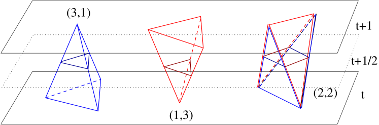
Figure 2: The three types of tetrahedral building blocks in three-dimensional CDT, and their intersections with the $t+1/2$ plane.

Note that a triangle is always shared by two tetrahedra, so that, for the number $N_{2}^{(s)}$ of spatial triangles, we have

$$N_{2}^{(s)}=\sum_{i=1}^{T}N_{2}(i)=\frac{1}{2}N_{(3,1)}\,,$$ (21)

which in the extended phase we expect to be roughly one third of the total volume $N_{3}$. For the value of $\kappa_{0}$ we used, the distribution of $N_{2}^{(s)}$ is very peaked (for $N_{3}=$100k the relative standard deviation is only $0.2\%$, see Fig. 3), and we find that $N_{(2,2)}$ is just slightly smaller than a third of the total volume.

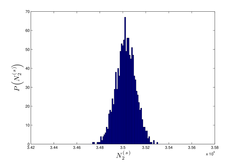
Figure 3: The distribution of the total number of spatial triangles $N_{2}^{(s)}$ (grouped in bins of size 10), for $N_{3}$=100k. The expectation value is $\langle N_{2}^{(s)}\rangle=35026$, with standard deviation $\sigma=85$.

In Fig. 4 we show the volume profile $N_{2}(i)$ from a snapshot of a Monte Carlo simulation. One notices immediately a phenomenon of spontaneous (translational) symmetry breaking: the Monte Carlo configuration shows a condensation of the volume around a specific time. Averaging over Monte Carlo configurations, the translational symmetry gets restored, but this is because a blind average amounts to summing over the degenerate vacua of the broken phase. As usual, in order to see spontaneous symmetry breaking we should select only one vacuum. For example, in a spin system this is done by first coupling the spins to an external magnetic field, which is then switched off. In the CDT simulations, we select one vacuum by performing a recentering of the Monte Carlo configurations. In practice, we have to find the center of volume $t_{CV}(j)$ for each Monte Carlo configuration $j$, and we have to shift time so that $t^{\prime}_{CV}(j)=T/2$ for every configuration in the new time variable. We performed this operation following the method given in Ambjorn:2008wc ; Gorlich:2011ga . Once the data are centered in this way, it makes sense to study the average of $N_{2}(i)$. A plot of $\langle N_{2}(i)\rangle$, together with fluctuations, is displayed in Fig. 5.

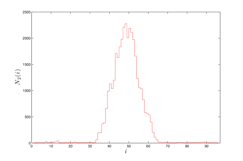
Figure 4: The spatial area $N_{2}(i)$ as a function of time, from a single configuration taken at random in the data set of Monte Carlo simulations for $N_{3}$=100k.

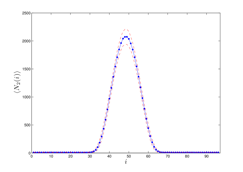
Figure 5: The mean spatial area as a function of discrete time, for $N_{3}$=100k. The blue dots represent the mean area $\langle N_{2}(i)\rangle$ of the volume data at time $i$, while the blue line is just an interpolation curve. Error bars (estimated for example by the jackknife method) are roughly of the size of the dot radii, or smaller, and thus we chose to omit them for clarity (this is done throughout the paper). The dashed red lines are interpolating curves for $\langle N_{2}(i)\rangle\pm\sigma/2$, where $\sigma=\sqrt{\langle(N_{2}(i))^{2}\rangle-\langle N_{2}(i)\rangle^{2}}$ is the size of the fluctuations.

The volume profile has a characteristic extended part (typically referred to as the blob or droplet), and a long flat tail (referred to as the stalk). Within the latter, the spatial volume is very close to its kinematical minimum, $\frac{1}{m}\sum_{i=1\ldots m}^{i\in{\rm stalk}}\langle N_{2}(i)\rangle\equiv n_{s}\sim 10$, and it is independent of the total volume. Most of the total volume is therefore concentrated in the blob. We will discuss in the following sections how to explain this condensation phenomenon, and which function best describes the volume profile.

3.2 The continuum limit

We conclude this section by discussing how the continuum limit $a\to 0$ is investigated on the basis of the simulation data. All observables and couplings in the simulations are given as dimensionless numbers, as such are also all the quantities appearing in (15) and the definition of the model. Length dimensions are introduced by multiplying the quantity of interest by the appropriate power of the cutoff $a$, the length of spacelike edges. For example, we can write $\tau=a\,\alpha\,T$ for the time interval, where we have introduced a parameter $\alpha>0$ to allow a different length of the timelike edges. Next, we can write $V_{2}=\frac{\sqrt{3}}{4}a^{2}N_{2}$ for the volume of a slice (the numerical prefactor being the area of an equilateral triangle of unit side), $V_{3}=v_{(3,1)}(\alpha)a^{3}N_{(3,1)}+v_{(2,2)}(\alpha)a^{3}N_{(2,2)}$ for the total volume, etc. Here, $v_{(3,1)}(\alpha)$ and $v_{(2,2)}(\alpha)$ stand for the volume of the $(3,1)$ and $(2,2)$ simplices with spatial edges of length one, and time edges of length $\alpha$ (they both coincide with the equilateral tetrahedron for $\alpha=1$, with volume $v_{3}=1/6\sqrt{2}$, see Ambjorn:2012jv ).

An essential part of the continuum limit procedure is to have $N\to\infty$ and $a\to 0$ in such a way that the physical volume

$$V\sim a^{d}N$$ (22)

remains finite. This implies that when we multiply a dimensionless quantity by $a^{n}$, in order to switch to its dimensional counterpart, in practice we multiply it by $N^{-n/d}$. For example, in CDT we also demand that $\tau\sim N^{-1/d}T$ stays finite.

In the thermodynamic limit we expect that, besides the total volume (22), also other dimensional large-scale observables will become independent of the cutoff $a$. Therefore, we expect to see scaling behavior when working with simulations at sufficiently large $N$, i.e. we expect that an observable $\langle\mathcal{O}(i)\rangle_{N}$, depending on the discrete time variable $i=1,\ldots,T$, will satisfy for some fixed (continuum time) $t$:

$$N^{-n/d}\langle\mathcal{O}(N^{1/d}t)\rangle_{N}=N^{\prime-n/d}\langle\mathcal{O}(N^{\prime 1/d}t)\rangle_{N^{\prime}}\,,$$ (23)

where the value of the observable at non-integer time is to be intended from an interpolating fit. The natural expectation would be that (22) and (23) hold with $n$ given by the expected dimension of the observable, but this is not guaranteed a priori and it is instead used as a check of the good classical properties of the model, as we do in the following. Moreover, not all quantities will show scaling: the dimensionless version of some quantity might remain independent of $N$. The typical example is the correlation length $l_{c}$, from $\langle\mathcal{O}(i)\mathcal{O}(j)\rangle_{N}-\langle\mathcal{O}(i)\rangle_{N}\langle\mathcal{O}(j)\rangle_{N}\sim e^{-|i-j|/l_{c}}$ (at large $|i-j|$); in order to obtain a finite dimensionful correlation length $\ell_{c}=al_{c}\sim N^{-1/d}l_{c}$, one needs to tune the couplings towards a critical point where $l_{c}$ diverges. We will not be concerned with correlation lengths here, but we will see another example of quantity that stays at the cutoff scale, i.e. the volume of the stalk in the droplet phase.

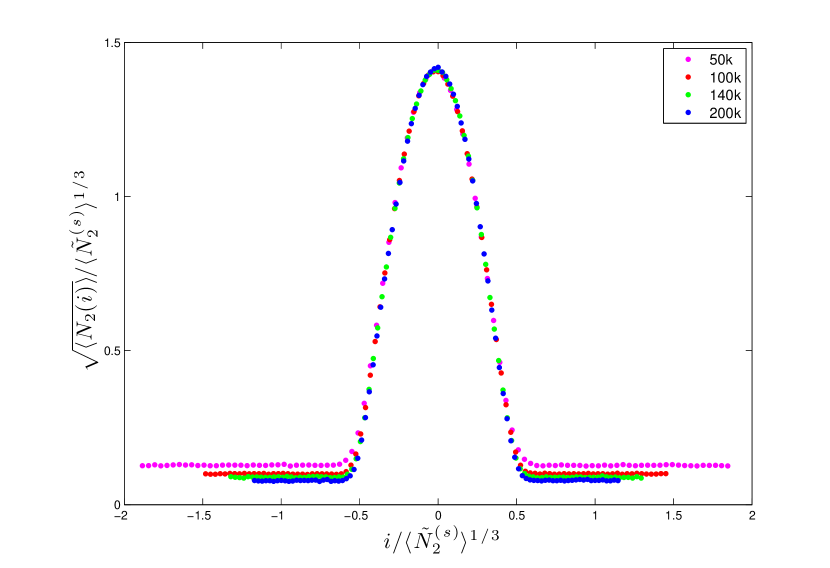
Figure 6: The square root of the mean spatial area as a function of discrete time (shifted so that the peak is at the origin). Both the mean area and the time variable are rescaled with the appropriate power of the average total volume $\tilde{N}_{2}^{(s)}=N_{2}^{(s)}-n_{s}T$, in order to display scaling.

Fig. 6 shows a scaling of the type (23). Here we have plotted $\langle N_{2}(i)\rangle^{1/2}/\langle\tilde{N}_{2}^{(s)}\rangle^{1/3}$ as a function of $i/\langle\tilde{N}_{2}^{(s)}\rangle^{1/3}$, for different data sets corresponding to different total volumes $N$. Following the procedure used in Ambjorn:2005qt , we used $\langle\tilde{N}_{2}^{(s)}\rangle=\langle N_{2}^{(s)}\rangle-n_{s}T$, instead of $\langle N_{2}^{(s)}\rangle$ (or $N_{3}$, which as we saw, is proportional to it) in the rescaling because we know that the volume in the stalk does not scale. The plot clearly shows that the superposition is extremely good inside the droplet, while in the stalk the rescaled volume goes to zero for growing $N_{3}$.

Another dynamical quantity that goes to zero in the continuum is the size of the fluctuations around the average, which we expect to be controlled by Newton’s constant. Indeed, without any fine tuning of the dimensionless couplings, all the couplings having positive (negative) length dimension will go to zero (infinity) as $a\to 0$. As Newton’s constant has the dimension of length for $d=3$, it is expected to go to zero in the naive continuum limit (in four spacetime dimensions, where Newton’s constant has dimension of length to the second power, this has been observed in Ambjorn:2008wc ). A finite coupling in the continuum could perhaps be attained by fine tuning the bare coupling to a second order phase transition.

4 Effective models

In this section we review how in four and (in more detail) three dimensions the dynamics of spatial volumes in CDT can be effectively described by BIB models. Minimization of the BIB model action, in accordance with its interpretation as a Landau free energy, leads to a good qualitative description of the full CDT phase diagram.

4.1 Four-dimensional CDT

In Bogacz:2012sa , Bogacz et al. studied a BIB model which is roughly a discretised version of a minisuperspace model corresponding to four-dimensional general relativity, and which was originally considered in Ambjorn:2004pw to explain the data from the simulations. It was found that this very simple model can account for many of the observed features of CDT in four dimensions, including its rich phase diagram. In particular, a droplet phase was found, which has remarkable similarities to the extended phase of CDT, although of course the comparison is limited to the behaviour of the spatial volume against time.

The model is defined by the following reduced transfer matrix,

$$g(m_{i},m_{i+1})=\exp\left(-c_{1}\frac{2(m_{i+1}-m_{i})^{2}}{m_{i}+m_{i+1}}-c_{2}\frac{m_{i}^{1/3}+m_{i+1}^{1/3}}{2}\right)\,.$$ (24)

In the continuum, this corresponds to the following action for the volume $V_{3}(t)$ of the 3-dimensional spatial slices,

$$S_{\rm 4d-mini}[V_{3}]=\frac{1}{2G}\int_{-\frac{\tau}{2}}^{\frac{\tau}{2}}dt\,\left(c_{1}\frac{\dot{V}_{3}^{2}(t)}{V_{3}(t)}+c_{2}V_{3}^{1/3}(t)\right)\,,$$ (25)

which is precisely of the type obtained from a minisuperspace reduction of general relativity (where $c_{1}=1/\mathcal{N}$, and $c_{2}=9(2\pi^{2})^{2/3}\mathcal{N}$, $\mathcal{N}$ being the lapse function). This is the action that was conjectured from the very beginning by Ambjorn et al. as an effective description for the extended part of the universe (or blob) in their simulations Ambjorn:2004pw , a conjecture which was further corroborated over the years Ambjorn:2005qt ; Ambjorn:2007jv ; Ambjorn:2008wc ; Ambjorn:2011ph . The novelty in Bogacz:2012sa was the suggestion that the same effective action can explain much more than just the dynamics inside the blob. Effectively, we can reinterpret the insight from Bogacz:2012sa as the observation that the BIB model with reduced transfer matrix (24) provides a good guess for a Landau free energy, i.e. in a bottom-up approach.

Notice that in the minisuperspace action that one would derive from the Einstein-Hilbert action the constant $c_{1}$ would be negative, while for a meaningful use of (25) as an effective action, and from comparison to the numerical data Ambjorn:2004pw , we must take it to be positive. It would thus seem that in CDT the conformal factor problem Gibbons:1978ac affecting Euclidean quantum gravity is solved, perhaps cured by nonperturbative contributions from the functional measure, as suggested in Dasgupta:2001ue . We will comment further on this below, arguing that in fact a simpler explanation is possible.

Another important difference between the usual minisuperspace model of general relativity and the BIB model, is that in the latter there is no analogue of the lapse to be integrated in the partition function and neither there is a summation/integration over $T$. As a consequence, there is no Hamiltonian constraint to be imposed in the semiclassical analysis. Above, we emphasised that the same situation should be expected in CDT, where the distance between one spatial slice and the next is constant and the total time extension of the universe is fixed in all simulations to date. This is also supported by the strong evidence from numerical simulations that the BIB model is a good effective description for CDT.

The equations of motion derived by varying (25) with respect to $V_{3}(t)$ are

$$c_{1}\left(\left(\frac{\dot{V}_{3}}{V_{3}}\right)^{2}-2\frac{\ddot{V}_{3}}{V_{3}}\right)+\frac{c_{2}}{3}\frac{1}{V_{3}^{2/3}}-\Lambda=0\,,$$ (26)

where the cosmological constant $\Lambda$ is introduced as a Lagrange multiplier, to be fixed by imposing the volume constraint. If we were to impose also the Hamiltonian constraint $H\equiv c_{1}\dot{V}_{3}^{2}(t)/V_{3}(t)-c_{2}V_{3}^{1/3}(t)+\Lambda V_{3}(t)=0$, the combined system of equations would reduce to a first order differential equation (by deriving the Hamiltonian constraint with respect to time, and eliminating $\ddot{V}_{3}(t)$ between the two equations). As such, its solutions would have only one free integration constant, which could be fixed for example by demanding that the maximum of $V_{3}(t)$ be at $t=0$. The solution would then be the “$\cos^{3}$” solution discussed by Ambjorn et al. in Ambjorn:2007jv ; Ambjorn:2008wc . However, without the Hamiltonian constraint the equation remains second-order, and thus there is one more free parameter, which allows us to perform a minimisation of the on-shell action.

For such a minimization one does not need to restrict to class $C^{2}(S^{1})$ functions, since for a well defined action (25) it is sufficient that $V_{3}(t)\in C^{1}(S^{1})$. This allows the authors of Bogacz:2012sa to consider droplet configurations that are not classical solutions, but that are expected on the basis of simulations and heuristic arguments. Using $V_{4}=\int_{-\frac{\tau}{2}}^{\frac{\tau}{2}}dtV_{3}(t)$ for the total volume in the continuum, they obtain the following expression for the dominant contribution to the path integral in a particular region of the the phase diagram:

$$\bar{V}_{3}(t)=\begin{cases}\frac{3\omega V_{4}}{4}\cos^{3}(\omega t)\,,&\text{for }t\in[-\frac{\pi}{2\omega},+\frac{\pi}{2\omega}]\,,\\ 0\,,&\text{for }t\in[-\frac{\tau}{2},-\frac{\pi}{2\omega})\cup(+\frac{\pi}{2\omega},+\frac{\tau}{2}]\,,\end{cases}$$ (27)

where

$$\omega=\frac{\sqrt{2}}{3V_{4}^{1/4}}\left(\frac{c_{2}}{c_{1}}\right)^{3/8}\,.$$ (28)

Notice that $V_{3}(t)=0$ obviously minimises the action (25) for positive $c_{1}$ and $c_{2}$. However, alone it would fail to satisfy the volume constraint, while a balance between the zero and the “$\cos^{3}$” solutions wins the energy balance, resulting in a condensation. Interestingly, the blob part of (27), together with (28), corresponds to the solution obtained by imposing also the Hamiltonian constraint, but this seems a mere coincidence.

The crucial point to be made here is that the presence of a potential term in (25) allows non-constant configurations such as (27) to dominate the path integral. Thus, the conclusions derived in this case are qualitatively different from those derived from (14) in the two-dimensional case.

The result is very interesting because it shows how the reduced model in four dimensions not only reproduces the extended part of the universe, but also its stalk, and it gives a prediction for their relative time extension.

It is also worth noticing that from the Einstein-Hilbert action the ratio $c_{2}/c_{1}$ would be fixed, thus leaving us with no parameters for a fit to the CDT simulations. Since the width of the universe (for fixed $V_{4}$) depends on the bare coupling $\kappa_{0}$ Ambjorn:2008wc , this is another indication that the effective action describing the volume dynamics is different form what would be expected from general relativity. We will now argue that such conclusion is even stronger in three dimensions.

4.2 Three-dimensional CDT

In three dimensions the minisuperspace reduction of the Einstein-Hilbert action contains no potential term, i.e. the action for the spatial areas in the proper-time gauge is exactly of the same form as (14), but with the length $L(t)$ replaced by the area of the spatial slices $V_{2}(t)$. As in the two-dimensional case, in the presence of a volume constraint $V_{3}=\int dtV_{2}(t)$ one finds oscillating solutions of the equations of motion, with a volume profile $V_{2}(t)\sim\cos^{2}(\omega t)$ which is compatible with the one observed inside the blob of Fig. 5. For this reason, such action has been suggested as an effective action for CDT Ambjorn:2000dja ; Ambjorn:2002nu (see also Cooperman:2013mma ). However, as pointed out in Benedetti:2014dra , in the light of the results on BIB models for two and four-dimensional CDT, the similarity of the general relativistic minisuperspace action in three dimensions to (14) immediately raises the question of how such an effective action could ever explain the important differences between two and three-dimensional CDT. Given that the two-dimensional case reduces exactly to a BIB model, and the four-dimensional case is well described (in its spatial volume dynamics) by a BIB model, we would expect a similar model to give also a good approximation for the three-dimensional model.

Of course an important difference between two and three dimensions is in the scaling of dimensionful quantities. Most importantly, Newton’s constant is dimensionless for $d=2$ while it has dimension of length for $d=3$. As a consequence, in the (naive, not fine-tuned) continuum limit, Newton’s constant (and with it the fluctuations around the average volume of the slices) scales to zero in the latter case, while it stays constant in the former. In two dimensions, as there are no other scales besides the cosmological one, the size of the fluctuations in the continuum limit is as large as the expectation value, thus blurring any classical behaviour. On the contrary, in three dimensions the fluctuations go to zero and the classical (mean field) behaviour should dominate.

Regardless of how the fluctuations behave, it turns out that the action derived from the Einstein-Hilbert action fails in reproducing the CDT results in an important way. Repeating the analysis of Bogacz et al. for three dimensions we simply have to set $c_{2}=0$ in the previous subsection, or just recall what we have said about the two-dimensional case. From (28) we then find that $\omega=0$, and the width of the droplet diverges. However, (28) does not hold in this case, as it would violate the condition $\pi/\omega<\tau$ which is to be assumed in (27). On the other hand we have already explained what happens in the two-dimensional case, and going to three dimensions we simply have to replace $V_{2}\to V_{3}$ and $\ell(t)\to V_{2}(t)$. The droplet solution which minimises the action is obtained for $\omega=\pi/\tau$. However, it is easily checked that in such a case the action is strictly positive, while for $V_{2}(t)=V_{3}/\tau$ the action vanishes. We conclude that a BIB model derived from the three-dimensional Einstein-Hilbert action would predict a constant average profile for the two-dimensional volumes. This is also supported by the numerical simulation of Bogacz:2012sa , as for $c_{2}=0$ and $c_{1}>0$ the model defined by (24) lies in the correlated fluid phase, not the droplet phase.

We are left with the challenge of explaining the droplet condensation of three-dimensional CDT as a condensation of a BIB model. This also provides us with an extraordinary opportunity to test corrections to the effective action of Ambjorn:2000dja ; Ambjorn:2002nu . In higher dimensions, such corrections are expected to be subdominant with respect to the the linear spatial curvature term coming from the Einstein-Hilbert action (the one multiplied by $c_{2}$ in (25)). Fortunately, however, the $d=3$ case is an exception to this, because this linear curvature term results in an irrelevant constant term for the potential, and hence drops out of the story, making higher order corrections relevant.

In view of that, and inspired by the reasonings outlined in the introduction, as well as by the fact that there is presently no evidence for the presence of higher-order time derivatives in the effective action Ambjorn:2011ph , in Benedetti:2014dra we proposed an alternative effective theory for the spatial areas, one derived from HL gravity.

Starting point: One sets off with the most generic, projectable, $z=2$ action for Hořava-Lifshitz gravity in three dimensions Horava:2008ih :

$$S_{\rm 3d-HL}=\frac{1}{16\pi G}\int\textrm{d}t\,\textrm{d}^{2}x\;\mathcal{N}\sqrt{g}\left\{(K_{ij}K^{ij}-\lambda K^{2})+2\Lambda-bR-\gamma R^{2}\right\}\,.$$ (29)

As discussed in the introduction, HL gravity describes a class of metric theories supporting a preferred foliation. Thus, the space-time diffeomorphism symmetry is broken down to foliation-preserving diffeomorphisms.

In (29), the action is presented in terms of ADM variables: $\mathcal{N}$ is the lapse function, $g$ is the determinant of the spatial metric, $R$ is its Ricci scalar, $K_{ij}$ is the extrinsic curvature associated to the leaves of the foliation, while $K$ is its trace.

The action contains the familiar parameter pair $(G,\Lambda)$, corresponding to Newton’s constant and the cosmological constant, respectively. The parameter $\sigma=\pm 1$ neatly encapsulates some metric signature information. Meanwhile $\lambda$, $b$ and $\gamma$ characterize the deviation from full diffeomorphism invariance. Indeed, for $\lambda=b=1$ and $\gamma=0$, one recovers the Einstein-Hilbert Lagrangian in Euclidean signature: $2\Lambda-\mathcal{R}$, where $\mathcal{R}$ is the spacetime Ricci tensor.

The theory is said to be projectable if one imposes at the outset that the lapse function is spatially constant: $\mathcal{N}=\mathcal{N}(t)$.

The $z$-exponent refers to half the maximal order of spatial derivatives appearing in the action. Thus for $z=2$, it may contain at most four spatial derivatives, permitting the inclusion of the $R^{2}$ term.

We consider spacetimes with topology $S^{2}\times S^{1}$, that is, spherical spatial slices and a compactified time. To implement this, we impose periodic boundary conditions in time, with period $\tau$.

Mini-superspace reduction: We perform a mini-superspace reduction to constant lapse, vanishing shift vector (hidden so far in the extrinsic curvature) and spatial metric $g_{ij}=\phi^{2}(t)\hat{g}_{ij}$, where $\hat{g}_{ij}$ is the standard metric on the unit sphere. And in order to compare to CDT in the canonical ensemble, we replace the cosmological term as:

$$\frac{2\Lambda}{16\pi G}\int\textrm{d}t\,\textrm{d}^{2}x\;\mathcal{N}\sqrt{g}\to\frac{2\Lambda}{16\pi G}\left(V_{3}-\int\textrm{d}t\,\textrm{d}^{2}x\;\mathcal{N}\sqrt{g}\right)\,,$$ (31)

and treat $\Lambda$ as a Lagrange multiplier.

With a redefinition of parameters, the action becomes:

$$S_{\textrm{3d-HL-mini}}[\phi]=\frac{1}{2\kappa^{2}}\int_{-\frac{\tau}{2}}^{\frac{\tau}{2}}\textrm{d}t\left\{\dot{\phi}^{2}-\omega^{2}\phi^{2}+b^{\prime}-\frac{\xi}{\phi^{2}}\right\}\,.$$ (33)

The remaining field $\phi(t)$ is a time-dependent scale factor determining the area of the spatial slice at time $t$: $V_{2}(t)=4\pi\phi^{2}(t)$. The constant $b^{\prime}$ term is clearly irrelevant for the problem of minimization of the action, and this can be traced back to the topological nature of the $R$ term in (29) for the projectable case.

The good sign of the action (a positive definite kinetic term) corresponds to $\kappa^{2}>0$, i.e. $\lambda<1/2$. However, in order to satisfy the periodic boundary conditions and to get real oscillating solutions, it turns out that one needs to take $\omega^{2}>0$ and $\xi>0$ (that is, an $R^{2}$ term with the bad sign), thus leading to a potential which is unbounded from below. Both sources of unboundedness are cured by (again CDT-inspired) constraints on the configuration space:

1. The unbounded $\phi^{2}$ term is tamed by the the fact that we are at fixed total volume, i.e. in the canonical ensemble. As the original $\Lambda$ above, $\omega^{2}$ should be treated as a Lagrange multiplier. The Euler-Lagrange equations for $\phi$ are unchanged, while variation with respect to the Lagrange multiplier imposes the constraint:

   $$\mathcal{V}\equiv 4\pi N\int_{-\frac{\tau}{2}}^{\frac{\tau}{2}}\textrm{d}t\,\phi^{2}(t)-V_{3}=0\,,$$ (34)

   that is, it fixes the 3-volume, and thus there is no unboundedness problem from the sign of the $\omega^{2}$ term.

2. The potential unboundedness stemming from the $1/\phi^{2}$ term is instead avoided by imposing a minimal spatial volume constraint at the outset, such as:

   $$\phi(t)>\epsilon\,,\quad\forall t\,.$$ (35)

   This can be thought as a regularization of the theory, and as discussed in Benedetti:2014dra , there are possible scaling limits to safely let $\epsilon\to 0$.

   Alternatively, we could think of the $1/\phi^{2}$ term in (33) as a truncation of the large-$\phi$ expansion of a potential that is not singular at $\phi=0$, e.g. $1/(\epsilon^{2}+\phi^{2})$.

Note that the constant lapse $\mathcal{N}$ has been neatly hidden away in (33). This is rather innocuous in a classical setting. But in principle, it is a degree of freedom that should be integrated over in a quantum regime leading to the imposition of a Hamiltonian constraint. Following Benedetti:2014dra , we shall not consider this scenario, rather setting $\mathcal{N}=1$ from here on. As we discussed above, that is appropriate when wishing to compare to CDT with fixed total time.

In order to rewrite, in analogy to the two and four-dimensional cases, the effective action in terms of area of the slices, we can simply change variables to:

$$V_{2}=4\pi\phi^{2}\,,$$ (36)

which comes from having assumed the slices to be 2-spheres of radius $\phi$. Leaving aside the constant term and the harmonic term, which is part of the volume constraint, one can rewrite (33) as:

$$\tilde{S}_{\textrm{3d-HL-mini}}[\phi]\equiv\frac{1}{2\kappa^{2}}\int_{-\frac{\tau}{2}}^{\frac{\tau}{2}}\textrm{d}t\left\{\dot{\phi}^{2}-\frac{\xi}{\phi^{2}}\right\}=\frac{1}{2\kappa^{2}}\int_{-\frac{\tau}{2}}^{\frac{\tau}{2}}\textrm{d}t\left\{\frac{1}{16\pi}\frac{\dot{V_{2}}^{2}}{V_{2}}-\frac{4\pi\xi}{V_{2}}\right\}\,\,.$$ (37)

BIB model and its phases: The action (37) is the form of the action that can most naturally be translated into a discrete BIB model of the type (6). The obvious discretization amounts to choosing the following reduced transfer matrix:

$$g(m_{j},m_{j+1})=\exp\left\{-\frac{2(m_{j+1}-m_{j})^{2}}{m_{j+1}+m_{j}}b_{1}+\frac{2}{m_{j+1}+m_{j}}b_{2}\right\}\,,$$ (38)

where $b_{1}$ and $b_{2}$ are parameters that can be related to the continuous ones, and the factors 2 remind us that we have chosen to write in the denominators the arithmetic mean of $m_{j}$ and $m_{j+1}$ (other choices, even non-symmetric, are possible, but are expected to be irrelevant in the continuum limit Bogacz:2012sa ).

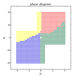
Figure 7: Phase diagram for the BIB model with reduced transfer matrix (38), with $T=80$ and $M=4000$: droplet (red triangles), localized (yellow squares), antiferromagnetic (blue pentagons), correlated fluid (green hexagons), and uncorrelated fluid (origin).

We performed Monte Carlo simulations of this BIB model in Benedetti:2016rwo , and we found evidence for five phases, whose location in the $(b_{1},b_{2})$ plane is illustrated in figure 7. Typical configurations for each phase are presented in figure 8, and they are characterized as follows (see Benedetti:2016rwo for more details):

• Droplet phase: This phase occurs for $b_{1}>0$, $b_{2}>b_{2,crit}(b_{1})$. For a typical configuration, the majority of volume condenses onto a contiguous subset of time slices of width greater than one. The remainder of the volume forms a stalk with each constituent time slice possessing minimal volume.

• Localized phase: This phase exists for $b_{1}<0$, $b_{2}>b_{2,crit}(b_{1})$. For a typical configuration, all volume resides on one time slice, while all other times possess minimal volume.

• Antiferromagnetic fluid phase: This phase exists for $b_{1}<0$, $b_{2}<b_{2,crit}(b_{1})$. A typical configuration consists of alternating peaks and troughs, where the troughs possess minimal volume.

• Correlated fluid phase: This phase exists for $b_{1}>0$, $b_{2}<b_{2,crit}(b_{1})$. A typical configuration consists of the volume approximately evenly allotted to the time slices, with relatively small fluctuations about the mean volume.

• Uncorrelated fluid phase: This phase exists near the origin, i.e. for $b_{1}\sim b_{2}\sim 0$, and probably only at the origin in the thermodynamic limit. It is a phase dominated by the entropy of configurations rather than by the action, which indeed vanishes at the origin, where the model is easily solved Bogacz:2012sa .

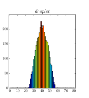
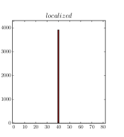
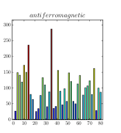
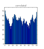
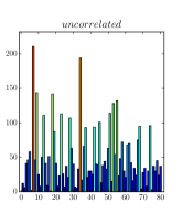
Figure 8: Typical configurations for the various phases (left-to-right): droplet, localized, antiferromagnetic, correlated fluid, uncorrelated fluid.

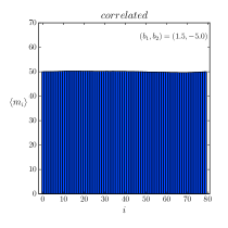
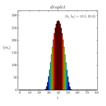
Figure 9: Mean value $\langle m_{i}\rangle$ as a function of $i$, for non-centred samples in the correlated phase and centred samples in the droplet phase.

Two of the phases above are akin to the two phases appearing in three-dimensional CDT, namely the droplet and the correlated phase. Clearly the former (see its averaged profile in Fig. 9) should correspond to the droplet configuration of Fig. 5, and we will get back to their comparison below. Notice also that although the typical configuration in the correlated phase shows relatively large fluctuation at our value of $M$ the ensemble average in figure 9 shows that they neatly average to a constant configuration. The antiferromagnetic and localized phases appear at negative kinetic term, and for this reason we will not discuss them further.

4.3 Analysis of the model

We can reverse the derivation of the BIB model and go back to the continuum, in order to look for the configurations that minimize the Landau free energy. First off, we notice that a three-dimensional interpretation of the BIB model is justified by the scaling observed in the droplet phase, see Fig. 10, which is of the same type as the scaling in the three-dimensional CDT model, see Fig. 6.

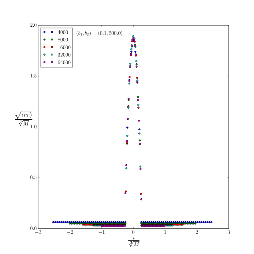
Figure 10: Scaling of averaged droplet with respect to volume $M$ (between 4k and 64k) at fixed $T=80$. We notice that rescaling both $\sqrt{\langle m_{i}\rangle}$ and $i$ with $\sqrt[3]{M}$, we obtain a droplet whose shape is essentially independent of $M$.

Let us introduce a lattice spacing $a$, and define a continuous time variable $t=aj$, with period $\tau=aT$. Furthermore, we define a continuous volume variable $V_{3}=v_{3}a^{3}M$, as well as interpret the number of balls in a given box $j$ as the two-dimensional volume of a slice at time $t$: $V_{2}=v_{2}a^{2}m$. Here, $v_{2}$ and $v_{3}$ are two arbitrary constants, that could be related to the details of the three-dimensional building blocks of CDT.

In the limit $a\to 0$, with $\tau$ and $V_{3}$ fixed, the exponent in (38) becomes the action

$$S[V_{2}]=\frac{1}{a}\int_{0}^{\tau}dt\left\{\frac{b_{1}}{v_{2}}\frac{\dot{V_{2}}^{2}}{V_{2}}-a^{2}b_{2}v_{2}\frac{1}{V_{2}}\right\}\,,$$ (39)

while the constraint on the total number of balls becomes the following volume constraint:

$$\int_{0}^{\tau}dtV_{2}=\frac{v_{2}}{v_{3}}V_{3}\,.$$ (40)

It is then natural to take $v_{2}=v_{3}\equiv v$.

The presence of the $1/a$ factor in front of the action (39) suggests that in the continuum limit the minimization of the action should provide a trustable approach to understanding the phase diagram of the BIB model. Note that it would be wrong to discard the potential term because of the $a^{2}$ multiplying it, because $V_{2}$ itself can be of order $a^{2}$.

A comparison of the actions (37) and (39) leads to the identifications:

$$\frac{1}{32\pi\kappa^{2}}=\frac{b_{1}}{av}\,,\;\;\;\frac{2\pi\xi}{\kappa^{2}}=ab_{2}v\,,$$ (41)

or:

$$\frac{b_{2}}{b_{1}}=\frac{64\pi^{2}\xi}{v^{2}a^{2}}\,.$$ (42)

One can eliminate any reference to the cutoff scale $a$ by looking only at dimensionless ratios of the parameters of the model. For example, using $va^{2}m_{min}=4\pi\epsilon^{2}$, one can write:

$$\frac{v\,b_{2}}{b_{1}m_{min}}=\frac{16\pi\xi}{\epsilon^{2}}\,.$$ (43)

In this way we can translate predictions from the continuum to the discrete.

For the continuum analysis, we will stick to the action in the $\phi$ parametrization, written as in (33) for deriving the equations of motion, and as in (37) for evaluating it on-shell (the $\omega^{2}$ term being part of the constraint it does not contribute to the on-shell action). The equations of motion derived from (33) are of Ermakov-Pinney type, i.e.:

$$\ddot{\phi}+\omega^{2}\phi-\frac{\xi}{\phi^{3}}=0\,,$$ (44)

and their solution is:

$$\phi_{0}(t)=\frac{1}{\omega A}\sqrt{(\omega^{2}A^{4}-\xi)\cos^{2}(\omega t+\psi)+\xi}\,,$$ (45)

where $A$ and $\psi$ are integration constants. Shifting the maximum of the curve to $t=0$ fixes $\psi=0$, and the maximal value $\phi_{0}(0)=A$ is then fixed by initial conditions. Meanwhile, the constraint $\mathcal{V}$ suffices to determine $\omega$ in terms of $\{V_{3},A,\xi\}$. However, notice that these solutions oscillate with period $\frac{\pi}{\omega}$, and therefore in order to satisfy periodic boundary conditions at $t=\pm\tau/2$, $\omega$ must also satisfy $\frac{\pi}{\omega}=\frac{\tau}{n}$ for some positive integer $n$. As a consequence, the space of solutions forms a discrete set.

These solutions never reach zero for $\xi>0$. This has ramifications for the space-time topology. In particular, it indicates the non-occurence of potential conical singularities, rather there is a minimal throat, at which the space-time bounces.

Besides the oscillating solutions, there is also a constant solution:

$$\bar{\phi}_{0}(t)=\sqrt{\frac{V_{3}}{4\pi\tau}}\,,$$ (46)

which is a special case of equation (45) with $A=\xi^{1/4}/\sqrt{\omega}$, and $\omega=4\pi\tau\sqrt{\xi}/V_{3}$ fixed by the volume constraint. This solution has special significance, since in comparison to the other local extrema, it has least action:

$$\tilde{S}_{\textrm{3d-HL-mini}}[\bar{\phi}_{0}]\leq\tilde{S}_{\textrm{3d-HL-mini}}[\phi_{0}]\,.$$ (48)

However, a standard second derivative test for constrained local extrema reveals that even the constant solution might not be a stable minimum for $\xi>0$ sufficiently large. Indeed the Hessian of (33) reads

$$\mathcal{H}(t,t^{\prime})=\left(-\partial_{t}^{2}-\omega^{2}-\frac{3\xi}{\phi(t)^{4}}\right)\delta(t-t^{\prime})\,,$$ (49)

and on the constant configuration it is diagonalized by the Fourier basis; as the tangent space to the constraint surface (34) at the constant solution is spanned by all the non-constant Fourier modes, we simply find that the condition for such a solution to be a minimum is

$$\left(\frac{2\pi n}{\tau}\right)^{2}-\omega^{2}-\frac{3\xi}{\bar{\phi}_{0}^{4}}=\left(\frac{2\pi n}{\tau}\right)^{2}-\frac{4\xi(4\pi\tau)^{2}}{V_{3}{}^{2}}>0\,,$$ (50)

which is violated (at least by the $n=1$ mode) as soon as $\xi>V_{3}{}^{2}/(16\tau^{4})$.

Keeping in mind that droplet-stalk configurations are of interest to us, we notice that the solutions (45) and (46) above capture fairly well the bulk of the droplet and the stalk, respectively. Therefore, with a touch of naiveté, let us graft the two together, and construct a configuration of the form:

$$\tilde{\phi}(t)=\left\{\begin{array}[]{lcl}\dfrac{1}{\omega A}\sqrt{(\omega^{2}A^{4}-\xi)\cos^{2}(\omega t)+\xi}&\textrm{for}&t\in[-\frac{\pi}{2\omega},+\frac{\pi}{2\omega}]\,,\\[8.5359pt] \dfrac{\sqrt{\xi}}{\omega A}&\textrm{for}&t\in[-\frac{\tau}{2},-\frac{\pi}{2\omega})\cup(+\frac{\pi}{2\omega},+\frac{\tau}{2}]\,,\\ \end{array}\right.$$ (51)

where one period of a configuration of the form (45) is confined to a subinterval of length $\pi/\omega<\tau$, while a constant configuration is attached in the remainder.

Such configurations are unusual for at least two reasons. First, they do not in general correspond to solutions of the Euler-Lagrange equations, except in the degenerate cases $A^{2}=(V_{3}+\sqrt{V_{3}^{2}-16\tau^{4}\xi})/(4\pi\tau)$, for which $\omega=\pi/\tau$, i.e. there is no stalk, and $A^{2}=\xi^{1/2}/\omega=V_{3}/(4\pi\tau)$, for which $\tilde{\phi}=\bar{\phi}_{0}$, i.e. there is no droplet. Second, they are only $C^{1}([-\tau/2,\tau/2])$, the second derivative being discontinuous at $t=\pm\frac{\pi}{2\omega}$. Nevertheless, we will now argue that they are relevant for the analysis of the model.

Local extrema vs absolute minima: The partition function of the system, in the continuum, reads:

$$Z_{\textrm{3d-HL-mini}}=\int_{\phi(t)>\epsilon}\mathcal{D}\phi(t)\,\delta(\mathcal{V})\,\exp\left\{-\frac{1}{2\kappa^{2}}\int_{-\frac{\tau}{2}}^{\frac{\tau}{2}}\textrm{d}t\left[\dot{\phi}^{2}-\frac{\xi}{\phi^{2}}\right]\right\}\,.$$ (52)

In the limit $\kappa\to 0$ we expect the partition function (and the observables) to be dominated by those configurations that minimize the action. Under the assumption that the space of field configurations is such that the action is at least differentiable (in the functional sense), there are two possible ways minima can arise: local extrema (i.e. solutions of the equations of motion) or minima lying on the boundary of configuration space. In the case that local extrema provide the dominant configurations for the path integral, this would imply dominance of the constant solution, because as we have seen this has the least action among all the solutions. On the other hand, if a configuration lying on the boundary of configuration space provides an absolute minimum, then we can have a non-constant profile. Such a possibility arises quite naturally in situations where an action unbounded from below is tamed by constraints. In our case, as we have already pointed out, the unboundedness of the action (37) at $\xi>0$ is tamed by the constraint (35), which introduces a boundary in configuration space. Therefore, absolute minima that are not local extrema can be expected. Indeed, it was argued in Benedetti:2014dra that this is precisely what gives rise to the droplet phase, with a profile of the form (51) dominating the partition function.

The rationale behind (51) is based on a balance between kinetic and potential terms in the action (created by their relative sign difference). If one looks at the kinetic term alone (at positive $b_{1}$, i.e. $\kappa^{2}$), then it is obvious that the minimizing configuration is a constant one, $\dot{\phi}(t)=0$. The volume constraint then fixes the value of $\phi(t)$ to (46). On the other hand, if one looks only at the potential term, then minimization would seem to push to a configuration with $\phi(t)=0$, leading to a singular value of the action which would clearly dominate over any other configuration (as long as $\dot{\phi}(t)$ stays finite). This is of course the instability caused by the unboundedness of the action, and as already repeatedly stressed it is cured by the constraint (35), as a consequence of which the potential actually favors the configuration $\phi(t)=\epsilon$. In fact, the volume constraint forbids a solution with $\phi(t)=\epsilon$ everywhere, but clearly if it were just for the potential term a delta-function configuration $V_{2}(t)=(V_{3}-4\pi\epsilon^{2}\tau)\,\delta(t-t_{0})+4\pi\epsilon^{2}$ would do the job, i.e. a localized configuration as seen in the top-right of Fig. 8, which indeed is found in particular at $b_{2}>0$ and $b_{1}=0$.

Therefore, for $\epsilon$ small enough, one sees a competition between the kinetic term, which favors the constant configuration, and the potential, which favors the delta-function configuration. What (51) envisages is a situation where the latter essentially wins, with the constant part being fixed at the minimal slice volume for the optimal choice of $A$, but with the kinetic term smoothing out the delta function, to a shape determined by local minimization of the action.

Phase transition: The discussion above was intended to provide a simple intuition of why a configuration such as (51) might dominate the path integral, but of course one has to explicitly check whether that is the case. The presence of several parameters and the fact that (34) leads to a cubic equation for $\omega$ complicate things, and in Benedetti:2014dra only a perturbative analysis for small $\epsilon$ and $\xi$ was presented.

Indeed plugging (51) into (34) we find:

$$V_{3}=4\pi\left(\frac{\pi(\xi+A^{4}\omega^{2})}{2A^{2}\omega^{3}}+\frac{\xi}{A^{2}\omega^{2}}\left(\tau-\frac{\pi}{\omega}\right)\right)\,,$$ (53)

which, multiplied by $\omega^{3}$ (non-zero otherwise we would have the constant solution again), gives us a cubic equation for $\omega$. It is convenient to rewrite the latter in terms of $\epsilon$ rather than $A$, taking $A=\sqrt{\xi}/(\epsilon\omega)$, because we expect the constant part to reach its minimal allowed value (from the considerations above, and from the perturbative analysis of Benedetti:2014dra ). We arrive at:

$$(4\pi\tau\epsilon^{4}-V_{3}\epsilon^{2})\omega^{3}-2\pi^{2}\epsilon^{4}\omega^{2}+2\pi^{2}\xi=0\,.$$ (54)

Although solvable, the general solution to such an equation is not very enlightening due to the presence of several parameters. We can gain some insight with some further assumptions on the nature of the roots. The discriminant of the cubic equation is:

$$-108\pi^{4}\xi^{2}\epsilon^{4}\left(V_{3}-4\pi\tau\epsilon^{2}\right)^{2}+64\pi^{8}\xi\epsilon^{12}\,,$$ (55)

and it has the following two roots when viewed as a function of $\xi$:

$$\xi_{1}=0\,,\;\;\;\text{and}\;\;\;\xi_{2}=\frac{16\pi^{4}\epsilon^{8}}{27\left(V_{3}-4\pi\tau\epsilon^{2}\right)^{2}}>0\,.$$ (56)

For small $\epsilon$ and large $V_{3}$, the positive root takes a very small value, and therefore we concentrate on the case $\xi>\xi_{2}$. In such case, the discriminant is negative and therefore the cubic equation has only one real root. Then we can use the representation of the real root in terms of hyperbolic functions, writing:

$$\omega_{0}=2\sqrt{\frac{-p}{3}}\cosh\left(\frac{1}{3}{\rm arcosh}\left(\frac{3q}{2p}\sqrt{-\frac{3}{p}}\right)\right)-\frac{a_{2}}{3a_{3}}\,,$$ (57)

where:

$$p=\frac{3a_{3}a_{1}-a_{2}^{2}}{3a_{3}^{2}}=-\frac{4\pi^{4}\epsilon^{4}}{3\left(V_{3}-4\pi\tau\epsilon^{2}\right)^{2}}\,,$$ (58)

$$q=\frac{27a_{3}^{2}a_{0}-9a_{3}a_{2}a_{1}+2a_{2}^{3}}{27a_{3}^{3}}=\frac{16\pi^{6}\epsilon^{8}-54\pi^{2}\xi\left(V_{3}-4\pi\tau\epsilon^{2}\right)^{2}}{27\epsilon^{2}\left(V_{3}-4\pi\tau\epsilon^{2}\right)^{3}}\,,$$ (59)

and $a_{n}$ is the coefficient of $\omega^{n}$ in the cubic equation (54). Furthermore, in (57) we have assumed $p<0$, $q<0$ and $4p^{3}+27q^{2}>0$, which are all valid for large enough $V_{3}$.

Lastly, we take (51) with $A=\sqrt{\xi}/(\epsilon\omega)$ and replace $\omega$ by the solution (57), to obtain a profile which is a function of $\xi$, $V_{3}$, $\tau$ and $\epsilon$. Denoting such configuration as $\hat{\phi}_{0}(t)$, we are interested in studying:

$$\mathcal{S}\equiv\tilde{S}_{\textrm{3d-HL-mini}}[\bar{\phi}_{0}]-\tilde{S}_{\textrm{3d-HL-mini}}[\hat{\phi}_{0}]$$ (60)

as a function of $\xi$, at fixed $\kappa^{2}$, $V_{3}$, $\tau$ and $\epsilon$, in order to check if and when the droplet configuration (51) dominates (i.e. $\mathcal{S}>0$).

More conveniently, we can re-express $\mathcal{S}$ in terms of the discrete BIB dimensionless parameters, eliminating $\xi$, $V_{3}$ and $\tau$ by means of the relations:

$$\frac{16\pi\xi}{\epsilon^{2}}=\frac{vb_{2}}{b_{1}m_{min}}\,,$$ (61)

$$\frac{V_{3}}{(4\pi\epsilon^{2})^{3/2}}=\frac{M}{m_{min}^{3/2}v^{1/2}}\,,$$ (62)

$$\frac{\tau}{(4\pi\epsilon^{2})^{1/2}}=\frac{T}{(m_{min}v)^{1/2}}\,.$$ (63)

One then finds that both $\epsilon$ and $\sqrt{v}$ factor out, so that $\mathcal{S}^{\prime}\equiv\kappa^{2}\mathcal{S}/(\epsilon\sqrt{v})$ depends only on the remaining discrete parameters. In particular, for $m_{min}=1$, $\mathcal{S}^{\prime}$ depends only on $M$, $T$ and the ratio $b_{2}/b_{1}$.

We thus come to our main conclusion: for fixed $M$ and $T$, the reasoning based on the minimization of the action predicts that there is a phase transition between a droplet ($\mathcal{S}>0$) and a correlated fluid phase ($\mathcal{S}<0$), with the boundary between the two phases being given by a straight line in the $(b_{1},b_{2})$ plane. In fact, for fixed $M$ and $T$, $\mathcal{S}^{\prime}$ is only a function of the ratio $\alpha\equiv b_{2}/b_{1}$, and the point at which $\mathcal{S}^{\prime}(\alpha_{c})=0$ corresponds to the phase transition. Unfortunately, such an equation cannot be solved in a closed form, and we are limited to a numerical evaluation of $\alpha_{c}$. For example, at $M=4000$ and $T=80$ , we find $\alpha_{c}=1.5$, while at $M=16000$ and $T=80$ , we find $\alpha_{c}=7.1$. We can also check numerically that at large volume $\alpha_{c}\propto M/T^{3}$. However, the quantitative predictions about the location of the phase transition should not be taken too seriously, because near the phase transition we expect the fluctuations to become important and affect the transition point.

The above results show that the droplet configuration (51) wins over the constant one in a certain range of parameters. What we have not shown is that there are no other solutions that win over both in that same range of parameters. In fact it is plausible that the actual dominant configuration is a smooth version of (51), i.e. one in which bulk and stalk are joined smoothly. However, we believe that the mechanism described above for our ansatz correctly captures the essential physical features of the problem, and this feeling is corroborated by the numerical simulations that have confirmed the existence of a droplet phase in the BIB model (6) with reduced transfer matrix (38).

5 Conclusions

In this review we have argued that the spatial volume profile in CDT can be interpreted as a sort of coarse grained order parameter, and that its associated Landau free energy can help us to understand the CDT phased diagram and the dynamics leading to it. At the same time it can also teach us something about the continuum limit, thanks to the partially local nature of such observable. Armed with such observable, and with the Landau theory point of view in mind, we have made the case that the continuum limit of CDT is most likely described by an FPD-invariant effective field theory, as in HL-type theories.

In particular, we have first reviewed the fact that in two-dimensional CDT the Landau free energy for the spatial length is obtained exactly and in the continuum limit it coincides with the two-dimensional HL gravity model. We have then argued that in order to explain the spacetime condensation phenomenon of three-dimensional CDT, reviewed in Sec. 3.1, a Landau free energy obtained as the discretization of a minisuperspace reduction of the Einstein-Hilbert action is not sufficient, as it would instead predict the dominance of a constant profile. By studying instead a Landau free energy inspired by HL gravity, proposed in Benedetti:2014dra , we have shown that a continuum semiclassical analysis leads to a condensation, captured by the dominant profile (51), compatible with the one observed in CDT. Such a semiclassical analysis is corroborated by the Monte Carlo simulations Benedetti:2016rwo of the effective BIB model, whose main results are summarized by the figures 7 and 11. The former shows the rich phase diagram of the BIB model proposed in Benedetti:2014dra . In particular, note the presence of a droplet phase, which however would be absent were one to set $b_{2}=0$, as in the BIB model related to minisuperspace reduction of general relativity. Figure 11 shows instead the excellent correspondence between the droplet phase of the BIB model and the CDT volume profile. Thus, we have compelling evidence that the effective dynamics of the CDT spatial slices is well captured by the BIB model (6)-(38), which in turn can be seen as a discretized path integral for a minusuperspace reduction of the Hořava-Lifshitz model (29).

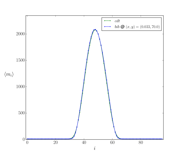
Figure 11: Comparison of the mean volume profile from the BIB model and three-dimensional CDT.

As we mentioned along the course of this review, there are a number of other reasons in support of a link between CDT and HL gravity (or more generally, FPD-invariant effective field theories). It is worth to collect them here in order to summarize the status of this relation:

• Presence of a foliation: This is on one hand a trivial observation, as it is a defining property of both CDT and HL gravity, and on the other a subtle one, as understanding the fate of the CDT foliation in the conitnuum limit is nontrivial. In particular, it is nontrivial because we have not yet identified a proper tuning towards the second-order phase transition that might lead to a continuum limit with propagating degrees of freedom (see Ambjorn:2014gsa ; Ambjorn:2020rcn for a first attempt). As a counterargument to the importance of the foliation, a generalized CDT model with a local causality constraint but no built-in foliation was introduced in Jordan:2013awa ; Jordan:2013iaa and shown to also lead to a semiclassical droplet phase with similar properties to that of standard CDT. On the other hand, even if such generalized CDT model would turn out to be indeed in the same universality class of usual CDT, this would not tell us what is their continuum interpretation: it might well be that the FPD-invariant universality class is robust under small departures from the foliated structure at the discrete level. Moreover, as argued in the introduction, the very fact that observables that are local in time are available and are being studied in CDT is by itself a signal of a likely departure from a full-diffeomorphism invariant theory.

• Analogies in the phase diagram: This was discussed for example in Ambjorn:2010hu , and it is based on the observation that a Lifshitz point is typically a tricritical point at the intersection of feromagnetic, paramagnetic and modulated phases, and that such phases, with their analog solutions in HL gravity, have a resemblance to the original three phases observed in four-dimensional CDT. The picture was slightly disturbed by the discovery of a new “bifurcation” phase in CDT Ambjorn:2014mra ; Ambjorn:2016mnn , but ultimately in our opinion its most concrete realization is in the kind of analysis we reviewed here: as reviewed in Sec. 4.2, the BIB model based on HL gravity leads to the phase diagram of Fig. 7, which at $b_{1}>0$ matches the phase diagram of CDT. A similar result holds also in four dimensions Bogacz:2012sa : in this case, no higher-order terms in the curvature are used, but nevertheless the fact that the coefficients of the kinetic and potential terms are tuned independently in order to reach the different phases suggests again a relation to HL gravity, as the ratio between the two would instead be fixed in the Einstein-Hilbert action. It would be interesting to add subleading terms in the potential of the BIB model for the four-dimensional case (see Ambjorn:2012pp for some results on such terms in CDT) to see if the new bifurcation phase of CDT can also be reproduced, although it has also been suggested that this might not be a conventional Landau-type phase transition Ambjorn:2020rcn .

• Short-scale spectral dimension: The fact that in the droplet phase of CDT the spectral dimension matches the classical value at (not too) large scales, and decreases at short scales Ambjorn:2005db was shown to be reproduced by HL gravity in Horava:2009if . However, several other approaches to quantum gravity claimed a similar result (e.g. in asymptotic safety Lauscher:2005qz ), thus weakening this point of contact. On the other hand, in Benedetti:2009ge it was pointed out that in three dimensions asymptotic safety and HL gravity give different predictions, and numerical evidence was produced in CDT favoring the HL scenario over the asymptotic safety one.

• Large-scale geometry: In Benedetti:2009ge it was also observed that the behavior of the spectral dimension at large scales, where it decays due to the compactness of spacetime, is better fitted by a stretched sphere geometry, rather than a round sphere. And the former is a solution to HL gravity.

• Absence of conformal factor problem: As we discussed in Sec. 4, the effective actions controlling the dynamics of the spatial volumes in CDT in $d=3$ and 4, have a kinetic term with the good sign, that is, there is no conformal sickness. While perhaps this could be interpreted as being due to nonperturbative contributions from the functional measure, as suggested in Dasgupta:2001ue , it might also have the much simpler explanation that in HL gravity the conformal factor problem can be avoided by an appropriate choice of the coupling $\lambda$ in (29). More investigations are probably needed in order to decide between the two scenarios, but one should keep in mind that if nonperturbative contributions could change the sign of the kinetic term for the conformal mode with respect to usual Euclidean quantum gravity Gibbons:1978ac , then either they would also spoil the good sign of the graviton term in the latter, or they would be hard to reconcile with general covariance of the theory, as the relative sign between conformal and graviton terms is fixed by full-diffeomorphism invariance. Unfortunately no results are available in CDT about a possible graviton effective action, but the possibility that only the conformal factor’s sign is changed with respect to usual Euclidean quantum gravity is corroborated by the results from three-dimensional CDT with toroidal slices Budd:2011zm , according to which both the conformal factor and the moduli have the good sign.

• Potential versus higher-derivatives: Results from Ambjorn:2011ph indicate that in four-dimensional CDT higher-order time derivatives in the effective action are subleading with respect to potential terms, that in a full action would correspond to higher-order spatial derivatives. This is suggestive again of an anisotropy.

• Exact relation in two dimensions: Lastly, two-dimensional CDT is exactly solvable and in the continuum limit it reproduces HL gravity, as reviewed in Sec. 2.3, and more in detail in Sato:2022ory . As there is currently no hint of a possible peculiarity of two dimensions when it comes to the CDT foliation, this makes a strong plausibility argument for a relation between CDT and HL gravity also in higher dimensions.

It should be stressed that clearly CDT in its usual definition has less couplings than renormalizable HL gravity models in three or four dimensions. Therefore, such renormalizable models are probably not directly relevant for comparisons to CDT, unless one extends the latter with appropriate new terms in the action, as done in Anderson:2011bj . However, as we argued in the introduction and in Sec. 2.3, the fact that one starts in CDT with a discretization of the Einstein-Hilbert action does not imply that its symmetries will be preserved. The crucial point, on which we focused in this review by indirect means, is to assess in which theory space a renormalization group flow of CDT will lead us, or in other words what is the effective field theory of CDT. Once that is established, only in a second step we will be able to worry about how to take the continuum limit with propagating degrees of freedom corresponding to our desired target theory. It is at this step that the fact that CDT has only few tunable parameters might turn out to be a limitation. At present, the two competing scenarios that can serve as justification for a program like CDT are asymptotic safety and HL gravity. While the latter is based on a Gaussian fixed point, and so it is straightforward to count the number of its relevant couplings, the former is based on a conjectural non-Gaussian fixed point, and we do not even know for sure if the number of relevant couplings is finite (except in special simple approximations Benedetti:2013jk ; Mitchell:2021qjr ). However, all evidence so far suggests that if such a nontrivial fixed point exists, then it has at least three relevant perturbations, which include higher-order curvature terms Codello:2008vh ; Benedetti:2009rx ; Falls:2014tra . Therefore, continuum scenarios and their results suggest that at some point one might need to introduce more couplings in CDT.

Lastly, we stress again that if indeed the effective field theory of CDT turns out to be a FPD-invariant one, this does not exclude the existence of a subspace of its theory space which is invariant under full diffeomorphisms. In other words, one might hope to embed asymptotically safe Euclidean gravity in the HL theory space. Reaching such subspace would probably require again a very delicate fine tuning of several breaking terms, yet perhaps in a less dramatic way than a full breaking of diffeomorphism invariance reuires, as in the functional renormalization group approach to asymptotic safety.

- (1) M. Aizenman and H. Duminil-Copin, Marginal triviality of the scaling limits of critical 4D Ising and models, Annals Math. 194 (2021) 163 [1912.07973].
- (2) S. Weinberg, ULTRAVIOLET DIVERGENCES IN QUANTUM THEORIES OF GRAVITATION, in General Relativity: An Einstein Centenary Survey, S.W. Hawking and W. Israel, eds., (Cambridge, UK), pp. 790–831, Univ. Pr. (1979).
- (3) M. Niedermaier and M. Reuter, The Asymptotic Safety Scenario in Quantum Gravity, Living Rev. Rel. 9 (2006) 5.
- (4) A. Bonanno, A. Eichhorn, H. Gies, J.M. Pawlowski, R. Percacci, M. Reuter et al., Critical reflections on asymptotically safe gravity, Front. in Phys. 8 (2020) 269 [2004.06810].
- (5) J. Ambjørn, B. Durhuus and T. Jonsson, Quantum Geometry: A Statistical Field Theory Approach, Cambridge Monographs on Mathematical Physics, Cambridge Univ. Press, Cambridge, UK (12, 2005), 10.1017/CBO9780511524417.
- (6) T. Regge, General relativity without coordinates, Nuovo Cim. 19 (1961) 558.
- (7) F. David, Planar Diagrams, Two-Dimensional Lattice Gravity and Surface Models, Nucl. Phys. B 257 (1985) 45.
- (8) J. Ambjorn, B. Durhuus and J. Frohlich, Diseases of Triangulated Random Surface Models, and Possible Cures, Nucl. Phys. B 257 (1985) 433.
- (9) V.A. Kazakov, A.A. Migdal and I.K. Kostov, Critical Properties of Randomly Triangulated Planar Random Surfaces, Phys. Lett. B 157 (1985) 295.
- (10) P. Di Francesco, P.H. Ginsparg and J. Zinn-Justin, Gravity and random matrices, Phys. Rept. 254 (1995) 1 [hep-th/9306153].
- (11) T. Budd, Lessons from the Mathematics of Two-Dimensional Euclidean Quantum Gravity, in Handbook of Quantum Gravity, C. Bambi, L. Modesto and I. Shapiro, eds., Springer Singapore (2023) [2212.03031].
- (12) B.V. de Bakker, Further evidence that the transition of 4-D dynamical triangulation is first order, Phys. Lett. B 389 (1996) 238 [hep-lat/9603024].
- (13) P. Bialas, Z. Burda, A. Krzywicki and B. Petersson, Focusing on the fixed point of 4-D simplicial gravity, Nucl. Phys. B 472 (1996) 293 [hep-lat/9601024].
- (14) J. Ambjorn and J. Jurkiewicz, Scaling in four-dimensional quantum gravity, Nucl. Phys. B 451 (1995) 643 [hep-th/9503006].
- (15) V. Bonzom, R. Gurau, A. Riello and V. Rivasseau, Critical behavior of colored tensor models in the large N limit, Nucl. Phys. B 853 (2011) 174 [1105.3122].
- (16) R. Gurau, Random Tensors, Oxford University Press, Oxford (2016).
- (17) J. Laiho and D. Coumbe, Evidence for Asymptotic Safety from Lattice Quantum Gravity, Phys. Rev. Lett. 107 (2011) 161301 [1104.5505].
- (18) D. Benedetti and R. Gurau, Phase Transition in Dually Weighted Colored Tensor Models, Nucl. Phys. B 855 (2012) 420 [1108.5389].
- (19) R. Gurau and J.P. Ryan, Melons are branched polymers, Annales Henri Poincare 15 (2014) 2085 [1302.4386].
- (20) V. Bonzom, Large Limits in Tensor Models: Towards More Universality Classes of Colored Triangulations in Dimension , SIGMA 12 (2016) 073 [1603.03570].
- (21) J. Ambjorn, L. Glaser, A. Goerlich and J. Jurkiewicz, Euclidian 4d quantum gravity with a non-trivial measure term, JHEP 10 (2013) 100 [1307.2270].
- (22) D. Coumbe and J. Laiho, Exploring Euclidean Dynamical Triangulations with a Non-trivial Measure Term, JHEP 04 (2015) 028 [1401.3299].
- (23) J. Laiho, S. Bassler, D. Coumbe, D. Du and J.T. Neelakanta, Lattice Quantum Gravity and Asymptotic Safety, Phys. Rev. D 96 (2017) 064015 [1604.02745].
- (24) J. Ambjorn and R. Loll, Nonperturbative Lorentzian quantum gravity, causality and topology change, Nucl. Phys. B 536 (1998) 407 [hep-th/9805108].
- (25) J. Ambjorn, J. Jurkiewicz and R. Loll, Dynamically triangulating Lorentzian quantum gravity, Nucl. Phys. B 610 (2001) 347 [hep-th/0105267].
- (26) J. Ambjorn, J. Jurkiewicz and R. Loll, Reconstructing the universe, Phys. Rev. D 72 (2005) 064014 [hep-th/0505154].
- (27) M. Visser, How to Wick rotate generic curved spacetime, 1702.05572.
- (28) A. Baldazzi, R. Percacci and V. Skrinjar, Wicked metrics, Class. Quant. Grav. 36 (2019) 105008 [1811.03369].
- (29) J. Ambjorn, S. Jordan, J. Jurkiewicz and R. Loll, Second- and First-Order Phase Transitions in CDT, Phys. Rev. D 85 (2012) 124044 [1205.1229].
- (30) J. Ambjorn, A. Goerlich, J. Jurkiewicz and R. Loll, Nonperturbative Quantum Gravity, Phys. Rept. 519 (2012) 127 [1203.3591].
- (31) R. Loll, Quantum Gravity from Causal Dynamical Triangulations: A Review, Class. Quant. Grav. 37 (2020) 013002 [1905.08669].
- (32) C. Rovelli, What Is Observable in Classical and Quantum Gravity?, Class. Quant. Grav. 8 (1991) 297.
- (33) S.B. Giddings, D. Marolf and J.B. Hartle, Observables in effective gravity, Phys. Rev. D 74 (2006) 064018 [hep-th/0512200].
- (34) J. Ambjorn, J. Jurkiewicz and R. Loll, Semiclassical universe from first principles, Phys. Lett. B 607 (2005) 205 [hep-th/0411152].
- (35) A. Dasgupta and R. Loll, A Proper time cure for the conformal sickness in quantum gravity, Nucl. Phys. B 606 (2001) 357 [hep-th/0103186].
- (36) P. Horava, Membranes at Quantum Criticality, JHEP 03 (2009) 020 [0812.4287].
- (37) P. Horava, Quantum Gravity at a Lifshitz Point, Phys. Rev. D 79 (2009) 084008 [0901.3775].
- (38) A. Wang, Hořava gravity at a Lifshitz point: A progress report, Int. J. Mod. Phys. D 26 (2017) 1730014 [1701.06087].
- (39) C.F. Steinwachs, Towards a unitary, renormalizable and ultraviolet-complete quantum theory of gravity, Frontiers in Physics 8 (2020) [2004.07842].
- (40) P. Horava, Spectral Dimension of the Universe in Quantum Gravity at a Lifshitz Point, Phys. Rev. Lett. 102 (2009) 161301 [0902.3657].
- (41) D. Benedetti and J. Henson, Spectral geometry as a probe of quantum spacetime, Phys. Rev. D 80 (2009) 124036 [0911.0401].
- (42) J. Ambjorn, A. Gorlich, S. Jordan, J. Jurkiewicz and R. Loll, CDT meets Horava-Lifshitz gravity, Phys. Lett. B 690 (2010) 413 [1002.3298].
- (43) T.G. Budd, The effective kinetic term in CDT, J. Phys. Conf. Ser. 36 (2012) 012038 [1110.5158].
- (44) J. Ambjørn, L. Glaser, Y. Sato and Y. Watabiki, 2d CDT is 2d Hořava–Lifshitz quantum gravity, Phys. Lett. B 722 (2013) 172 [1302.6359].
- (45) D. Benedetti and J. Henson, Spacetime condensation in (2+1)-dimensional CDT from a Hořava–Lifshitz minisuperspace model, Class. Quant. Grav. 32 (2015) 215007 [1410.0845].
- (46) D. Benedetti and J.P. Ryan, Capturing the phase diagram of (2 + 1)-dimensional CDT using a balls-in-boxes model, Class. Quant. Grav. 34 (2017) 105012 [1612.09533].
- (47) C. Anderson, S.J. Carlip, J.H. Cooperman, P. Horava, R.K. Kommu and P.R. Zulkowski, Quantizing Horava-Lifshitz Gravity via Causal Dynamical Triangulations, Phys. Rev. D 85 (2012) 044027 [1111.6634].
- (48) M. Borji and C. Kopper, Perturbative renormalization of the lattice regularized with flow equations, J. Math. Phys. 61 (2020) 112304 [2006.15943].
- (49) M. Testa, The Rome approach to chirality, in APCTP - ICTP Joint International Conference (AIJIC 97) on Recent Developments in Nonperturbative Quantum Field Theory, pp. 114–127, 7, 1997 [hep-lat/9707007].
- (50) J. Magnen, V. Rivasseau and R. Seneor, Construction of Y M(4) with an infrared cutoff, Commun. Math. Phys. 155 (1993) 325.
- (51) U. Ellwanger, Flow equations and BRS invariance for Yang-Mills theories, Phys. Lett. B 335 (1994) 364 [hep-th/9402077].
- (52) H. Gies, Introduction to the functional RG and applications to gauge theories, Lect. Notes Phys. 852 (2012) 287 [hep-ph/0611146].
- (53) N. Goldenfeld, Lectures on phase transitions and the renormalization group, CRC Press (1992).
- (54) D.A. Johnston, J.P. Kownacki and A. Krzywicki, Random geometries and real space renormalization group, Nucl. Phys. B Proc. Suppl. 42 (1995) 728 [hep-lat/9407018].
- (55) G. Thorleifsson and S. Catterall, A real space renormalization group for random surfaces, Nucl. Phys. B 461 (1996) 350 [hep-lat/9510003].
- (56) J. Ambjorn, P. Bialas and J. Jurkiewicz, RG flow in an exactly solvable model with fluctuating geometry, Phys. Lett. B 379 (1996) 93 [hep-lat/9602021].
- (57) R.L. Renken, A Renormalization group for dynamical triangulations in arbitrary dimensions, Nucl. Phys. B 485 (1997) 503 [hep-lat/9607074].
- (58) J. Henson, Coarse graining dynamical triangulations: A New scheme, Class. Quant. Grav. 26 (2009) 175019 [0907.5602].
- (59) F. Markopoulou, Coarse graining in spin foam models, Class. Quant. Grav. 20 (2003) 777 [gr-qc/0203036].
- (60) R. Oeckl, Renormalization of discrete models without background, Nucl. Phys. B 657 (2003) 107 [gr-qc/0212047].
- (61) B. Bahr, B. Dittrich, F. Hellmann and W. Kaminski, Holonomy Spin Foam Models: Definition and Coarse Graining, Phys. Rev. D 87 (2013) 044048 [1208.3388].
- (62) B. Dittrich, M. Martín-Benito and E. Schnetter, Coarse graining of spin net models: dynamics of intertwiners, New J. Phys. 15 (2013) 103004 [1306.2987].
- (63) S. Steinhaus, Coarse Graining Spin Foam Quantum Gravity—A Review, Front. in Phys. 8 (2020) 295 [2007.01315].
- (64) R.L. Renken, S.M. Catterall and J.B. Kogut, Phase structure of dynamical triangulation models in three-dimensions, Nucl. Phys. B 523 (1998) 553 [hep-lat/9712011].
- (65) P. Bialas, Z. Burda and D. Johnston, Phase diagram of the mean field model of simplicial gravity, Nucl. Phys. B 542 (1999) 413 [gr-qc/9808011].
- (66) M.R. Evans and T. Hanney, Nonequilibrium statistical mechanics of the zero-range process and related models, J. Phys. A: Math. and Gen. 38 (2005) R195.
- (67) P. Bialas, Z. Burda, B. Petersson and J. Tabaczek, Appearance of mother universe and singular vertices in random geometries, Nucl. Phys. B 495 (1997) 463 [hep-lat/9608030].
- (68) P. Bialas, Z. Burda and D. Johnston, Condensation in the backgammon model, Nucl. Phys. B 493 (1997) 505 [cond-mat/9609264].
- (69) L. Bogacz, Z. Burda and B. Waclaw, Quantum widening of CDT universe, Phys. Rev. D 86 (2012) 104015 [1204.1356].
- (70) M.R. Evans, T. Hanney and S.N. Majumdar, Interaction-driven real-space condensation, Phys. Rev. Lett. 97 (2006) 010602.
- (71) B. Waclaw, J. Sopik, W. Janke and H. Meyer-Ortmanns, Tuning the shape of the condensate in spontaneous symmetry breaking, Phys. Rev. Lett. 103 (2009) 080602 [0901.3664].
- (72) P. Di Francesco, E. Guitter and C. Kristjansen, Integrable 2-D Lorentzian gravity and random walks, Nucl. Phys. B 567 (2000) 515 [hep-th/9907084].
- (73) P. Di Francesco, E. Guitter and C. Kristjansen, Generalized Lorentzian triangulations and the Calogero Hamiltonian, Nucl. Phys. B 608 (2001) 485 [hep-th/0010259].
- (74) P. Di Francesco and E. Guitter, Critical and multicritical semirandom (1+d)-dimensional lattices and hard objects in d-dimensions, J. Phys. A 35 (2002) 897 [cond-mat/0104383].
- (75) A.K. Murtazaev and Z.G. Ibaev, On choosing the order parameter of modulated magnetic structures, Journal of Experimental and Theoretical Physics 116 (2013) 266.
- (76) Y. Sato, CDT and Horava-Lifshitz QG in Two Dimensions, in Handbook of Quantum Gravity, C. Bambi, L. Modesto and I. Shapiro, eds., Springer Singapore (2023) [2212.03446].
- (77) F. Mattei, C. Rovelli, S. Speziale and M. Testa, From 3-geometry transition amplitudes to graviton states, Nucl. Phys. B 739 (2006) 234 [gr-qc/0508007].
- (78) J. Ambjorn, K.N. Anagnostopoulos and R. Loll, A New perspective on matter coupling in 2-D quantum gravity, Phys. Rev. D 60 (1999) 104035 [hep-th/9904012].
- (79) J. Ambjørn, A. Görlich, J. Jurkiewicz and H. Zhang, The microscopic structure of 2D CDT coupled to matter, Phys. Lett. B 746 (2015) 359 [1503.01636].
- (80) J. Ambjorn, J. Jurkiewicz, R. Loll and G. Vernizzi, Lorentzian 3-D gravity with wormholes via matrix models, JHEP 09 (2001) 022 [hep-th/0106082].
- (81) D. Benedetti, R. Loll and F. Zamponi, (2+1)-dimensional quantum gravity as the continuum limit of Causal Dynamical Triangulations, Phys. Rev. D 76 (2007) 104022 [0704.3214].
- (82) J. Ambjorn, J. Jurkiewicz and R. Loll, Nonperturbative 3-D Lorentzian quantum gravity, Phys. Rev. D 64 (2001) 044011 [hep-th/0011276].
- (83) J.H. Cooperman and J. Miller, A first look at transition amplitudes in (2 + 1)-dimensional causal dynamical triangulations, Class. Quant. Grav. 31 (2014) 035012 [1305.2932].
- (84) T.G. Budd and R. Loll, Exploring Torus Universes in Causal Dynamical Triangulations, Phys. Rev. D 88 (2013) 024015 [1305.4702].
- (85) J. Ambjorn, A. Gorlich, J. Jurkiewicz and R. Loll, The Nonperturbative Quantum de Sitter Universe, Phys. Rev. D 78 (2008) 063544 [0807.4481].
- (86) A. Gorlich, Causal Dynamical Triangulations in Four Dimensions, Ph.D. thesis, Jagiellonian U., Astron. Observ., 2010. 1111.6938.
- (87) J. Ambjorn, A. Gorlich, J. Jurkiewicz and R. Loll, Planckian Birth of the Quantum de Sitter Universe, Phys. Rev. Lett. 100 (2008) 091304 [0712.2485].
- (88) J. Ambjorn, A. Gorlich, J. Jurkiewicz, R. Loll, J. Gizbert-Studnicki and T. Trzesniewski, The Semiclassical Limit of Causal Dynamical Triangulations, Nucl. Phys. B 849 (2011) 144 [1102.3929].
- (89) G.W. Gibbons, S.W. Hawking and M.J. Perry, Path Integrals and the Indefiniteness of the Gravitational Action, Nucl. Phys. B 138 (1978) 141.
- (90) J. Ambjorn, J. Jurkiewicz and R. Loll, 3-d Lorentzian, dynamically triangulated quantum gravity, Nucl. Phys. B Proc. Suppl. 106 (2002) 980 [hep-lat/0201013].
- (91) J. Ambjorn, A. Görlich, J. Jurkiewicz, A. Kreienbuehl and R. Loll, Renormalization Group Flow in CDT, Class. Quant. Grav. 31 (2014) 165003 [1405.4585].
- (92) J. Ambjorn, J. Gizbert-Studnicki, A. Görlich, J. Jurkiewicz and R. Loll, Renormalization in quantum theories of geometry, Front. in Phys. 8 (2020) 247 [2002.01693].
- (93) S. Jordan and R. Loll, Causal Dynamical Triangulations without Preferred Foliation, Phys. Lett. B 724 (2013) 155 [1305.4582].
- (94) S. Jordan and R. Loll, De Sitter Universe from Causal Dynamical Triangulations without Preferred Foliation, Phys. Rev. D 88 (2013) 044055 [1307.5469].
- (95) J. Ambjørn, J. Gizbert-Studnicki, A. Görlich and J. Jurkiewicz, The effective action in 4-dim CDT. The transfer matrix approach, JHEP 06 (2014) 034 [1403.5940].
- (96) J. Ambjørn, J. Gizbert-Studnicki, A. Görlich, J. Jurkiewicz, N. Klitgaard and R. Loll, Characteristics of the new phase in CDT, Eur. Phys. J. C 77 (2017) 152 [1610.05245].
- (97) J. Ambjorn, J. Gizbert-Studnicki, A. Gorlich and J. Jurkiewicz, The Transfer matrix in four-dimensional CDT, JHEP 09 (2012) 017 [1205.3791].
- (98) J. Ambjorn, J. Jurkiewicz and R. Loll, Spectral dimension of the universe, Phys. Rev. Lett. 95 (2005) 171301 [hep-th/0505113].
- (99) O. Lauscher and M. Reuter, Fractal spacetime structure in asymptotically safe gravity, JHEP 10 (2005) 050 [hep-th/0508202].
- (100) D. Benedetti and F. Guarnieri, One-loop renormalization in a toy model of Hořava-Lifshitz gravity, JHEP 03 (2014) 078 [1311.6253].
- (101) A.O. Barvinsky, D. Blas, M. Herrero-Valea, S.M. Sibiryakov and C.F. Steinwachs, Hořava Gravity is Asymptotically Free in 2 + 1 Dimensions, Phys. Rev. Lett. 119 (2017) 211301 [1706.06809].
- (102) A.O. Barvinsky, M. Herrero-Valea and S.M. Sibiryakov, Towards the renormalization group flow of Horava gravity in dimensions, Phys. Rev. D 100 (2019) 026012 [1905.03798].
- (103) A.O. Barvinsky, A.V. Kurov and S.M. Sibiryakov, Beta functions of (3+1)-dimensional projectable Hořava gravity, Phys. Rev. D 105 (2022) 044009 [2110.14688].
- (104) D. Benedetti, On the number of relevant operators in asymptotically safe gravity, EPL 102 (2013) 20007 [1301.4422].
- (105) A. Mitchell, T.R. Morris and D. Stulga, Provable properties of asymptotic safety in f(R) approximation, JHEP 01 (2022) 041 [2111.05067].
- (106) A. Codello, R. Percacci and C. Rahmede, Investigating the Ultraviolet Properties of Gravity with a Wilsonian Renormalization Group Equation, Annals Phys. 324 (2009) 414 [0805.2909].
- (107) D. Benedetti, P.F. Machado and F. Saueressig, Asymptotic safety in higher-derivative gravity, Mod. Phys. Lett. A 24 (2009) 2233 [0901.2984].
- (108) K. Falls, D.F. Litim, K. Nikolakopoulos and C. Rahmede, Further evidence for asymptotic safety of quantum gravity, Phys. Rev. D 93 (2016) 104022 [1410.4815].