Superfluid excitations in a rotating two-dimensional bubble trap

Abstract

We studied a rotating BEC confined in a bubble trap, approximated by a Mexican hat and shifted harmonic oscillator potentials. Using a variational technique and perturbation theory, we determined the vortex configurations in this system by varying the interparticle interaction and the angular velocity of the atomic cloud. We found that the phase diagram of the system has macrovortex structures for small positive values of the interaction parameter, and the charge of the central vortex increases with rotation. Strengthening the atomic interaction makes the macrovortex unstable and decays into multiple singly-charged vortices that arrange themselves in a lattice configuration. We also look for experimentally realizable methods to determine the vortex configuration without relying upon absorption imaging since the structures are not always visible in the latter. More specifically, we study how the vortex distribution affects the collective modes of the condensate by solving the Gross-Pitaevskii equation numerically and by analytical predictions using the sum-rule approach for the frequencies of the modes. These results reveal important signatures to characterize the macrovortices and vortex lattice transitions in the experiments.

I Introduction

The behavior of a quantum gas, while sharing many similarities with its classical counterpart, differs dramatically from it when subject to rotation. A classical gas under rotation develops a rigid body velocity field Landau and Lifshitz (1976), propelled by the centrifugal effects as seen in the laboratory frame. In contrast, a quantum gas might excite collective modes or, in some situations, develop one or more quantized vortices: lines of vanishing density around which the phase of the condensate changes by an integer multiple of $2\pi$ Pitaevskii and Stringari (2016); Pethick and Smith (2008). Early experiments in the field used harmonic potentials to trap the gas Anderson et al. (1995); Davis et al. (1995); Bradley et al. (1995). This naturally imposes a limit on the rotation frequency, as the centrifugal effects weaken the confinement of the trap. For sufficiently large angular velocities, multiple vortices develop in the bulk of the condensate, and the gas becomes populated by a vortex lattice Abo-Shaeer et al. (2001); Butts and Rokhsar (1999), with the average velocity field due to the many vortices mimicking a rigid body velocity field. For even higher velocities, the system is expected to enter a highly degenerate state known as the lowest Landau level Fetter (2008), with a Hamiltonian mathematically equivalent to the one of an electron moving in a 2D uniform magnetic field, in the context of the quantum Hall effect Tong (2016).

Producing high angular velocities is experimentally challenging since the harmonic trap confinement gets weaker when approaching this regime due to centrifugal effects. This feature attracted research interest in potentials with a stronger than harmonic confinement, where this critical, deconfining angular velocity could be approached or even surpassed. A popular stronger than harmonic trap was the quartic potential Danaila (2005); Cozzini (2006); Fetter (2001), where in addition to dense vortex lattices, giant, multi-quantized vortices called macrovortices or giant vortices were also predicted and observed Fu and Zaremba (2006); Aftalion and Danaila (2004).

In this context, a very rich potential under theoretical and experimental scrutiny is the bubble trap potential, proposed by Garraway and Zobay in 2001 Zobay and Garraway (2001, 2004). The bubble trap is an adiabatic potential formed by superpositioning a static inhomogeneous magnetic field with a spatially homogeneous radio frequency (RF). This confines the atoms to an isomagnetic surface. In typical experiments, gravity cannot be neglected, and the resulting equilibrium configuration pools the atoms at the bottom of the surface Colombe et al. (2004); Garraway and Perrin (2016).

Besides providing stronger than harmonic confinement for the condensate, the bubble trap also allows for control over the topology of the system. By varying the parameters of the field, one can control how strongly the atoms are confined to the isomagnetic surface. This allows for studying nearly two-dimensional (2D) gases bound to surfaces Perrin and Garraway (2017). The topology has non-trivial consequences over many properties of the gas. We mention, for instance, the effects of the dimensionality over the condensation temperature, which are already notorious Pitaevskii and Stringari (2016); Pethick and Smith (2008). Padavic and Sun analyzed how the collective modes of a spherical condensate change when it transitions from a filled to a hollow sphere, finding a dip in the breathing modes and a restructuring in the surface modes due to the emergence of a second interior surface Padavić et al. (2018); Sun et al. (2018).

As with the quartic potential and in contrast to the harmonic potential, because the energy of single particle states varies faster than linearly with angular momentum when confined to the bubble trap, the condensate can accommodate macrovortices as well as vortex lattices Lundh (2002); Jackson et al. (2004). However, the experimental status of these predictions remains to be determined: the dense vortex lattice expected to be seen close to the critical rotation frequency was not observed Herve (2018). When using the bubble trap to form a ring, an unstable charge $3$ vortex has been observed to split into $3$ unit charge vortices de Goër de Herve et al. (2021). Moreover, ongoing experimental efforts exist to realize the bubble trap in microgravity conditions aboard the Cold Atom Laboratory in the International Space Station. In the future, a rotating version of the experiment is expected Carollo et al. (2022).

These facts emphasize the need to understand how the vortex charge and charge distribution behave with varying rotation and interaction strengths under the bubble trap potential, a situation we seek to address in this work. We study vortex configurations for a rotating gas confined in a bubble trap, approximating it by the Mexican hat (MH) and shifted harmonic oscillator potentials (SHO). Using a variational technique and numerical methods, we construct a phase diagram studying the total vortex charge and charge distribution as the interaction parameter and the angular velocity of the gas vary. We make predictions for discontinuous first-order transitions, where the total vortex charge increases, and continuous second-order transitions, where only the charge distribution varies. For weak interactions and low rotation speeds, the system is characterized by a central macrovortex, but as interaction increases, it breaks into multiple charge $1$ vortices. The shifted harmonic oscillator potential can withstand a broader range of interaction parameters before breaking the macrovortex compared to the Mexican hat potential. We also develop sum rules and numerical predictions using real and imaginary time simulations of the Gross–Pitaevskii equation (GPE) for the monopole and quadrupole collective modes of the gas, searching for a signature of the charge and charge distribution of vortices. We find that monopole frequencies increase with rotation only when there is a corresponding increase in vortex charge, and it is larger for a vortex lattice than for a macrovortex. At the same time, there is a frequency split proportional to the total angular momentum between quadrupole modes co and anti-rotating with the gas.

This work is structured as follows: in Sec. II.1, we present the bubble trap. Since dealing directly with this potential can be complicated, we also discuss two approximations — the Mexican hat and the shifted harmonic oscillator, or ring trap potential. Then, in Sec. II.2, we present the total Hamiltonian of the system, including rotation, from which we compute the energy of the system. This energy is minimized using a functional space described in Sec. III, where we also present our results for the MH and SHO potentials. Seeking experimental alternatives to characterize the vortex configurations of the gas, in Sec. IV we introduce the sum rules formalism for evaluating the monopole and two-dimensional quadrupole collective modes, with special attention to how the vortex configuration affects these frequencies. Finally, we present our conclusions in Sec. V. In the Appendices, we provide more details on the derivation of results reported in the main text related to the virial theorem (Appendix A), compressibility sum rules (Appendix B) and the calculation of some relevant moments (Appendix C).

II Bubble trap with rotation

II.1 Bubble trap

Experimentally, a bubble trap can be constructed by combining a linearly or circularly polarized RF magnetic field and an inhomogeneous static magnetic field. Suppose an atom possessing a fine structure interacts with this setting. Particles will be attracted or repelled from areas of low magnetic fields, depending on their spin orientation. Then for some atoms, there will be a region of space where the split energy levels due to the Zeeman effect will resonate with the applied radio frequency, causing the spin state to change to its opposite. Therefore the potential landscape experienced by the particle will be inverted: it will now be attracted or repelled from areas of higher magnetic field and cross the region again. If their velocity is small enough, they oscillate around this region, trapped close to an isomagnetic surface.

In particular, the isomagnetic surface of an ellipsoid of revolution is generated by combining a quadrupole static magnetic field and an RF field. Under adiabatic conditions, i.e., if atoms cross the region with small enough velocities, it can be shown that an expression of the potential is given by Perrin and Garraway (2017):

$$\tilde{V}_{\textrm{Bubble}}(r)=M_{F}\sqrt{\left(\frac{1}{2}\frac{\tilde{M}\tilde{\omega}_{0}^{2}\tilde{r}^{2}}{2}-\hbar\tilde{\Delta}\right)^{2}+(\hbar\tilde{\Theta})^{2}},$$ (1)

where $\tilde{\Delta}$ corresponds to the detuning between the applied RF field and the energy states, and $\tilde{\Theta}$ is the Rabi coupling between these states. In the limit $\tilde{\Delta}=\tilde{\Theta}=0$, the potential of Eq. (1) reduces to a usual harmonic oscillator trap. On the other hand, for large $\tilde{\Delta}$, it can be approximated near its minimum by a radially shifted harmonic trap with frequency $\tilde{\omega}_{\rm SHO}=({M_{F}\tilde{\Delta}}/{\tilde{\Theta}})^{1/2}\tilde{\omega}_{0}$.

Hereafter we reserve the tilde notation for quantities with dimensions. Dimensionless quantities are constructed considering $r\equiv\tilde{r}/{\tilde{\ell}_{0}}$ (with $\tilde{\ell}_{0}\equiv[{\hbar}/({\tilde{M}\tilde{\omega}_{0})}]^{1/2}$), $\Theta\equiv\tilde{\Theta}/{\tilde{\omega}_{0}}$, $\Delta\equiv\tilde{\Delta}/{\tilde{\omega}_{0}}$, and energies in units of $\hbar\tilde{\omega}_{0}$. Choosing the atomic hyperfine state $M_{F}=2$ yields

$$V_{\textrm{Bubble}}(r)=2\sqrt{\left(\frac{r^{2}}{4}-\Delta\right)^{2}+\Theta^{2}},$$ (2)

with a trap minimum corresponding to $r_{\rm min}=2\sqrt{\Delta}$.

We considered two limits of the bubble trap potential. For that, it is convenient to rewrite Eq. (2) in terms of $r_{\rm min}$,

$${V}_{\textrm{Bubble}}({r})=\frac{r_{\rm min}^{2}}{2}\sqrt{\left(\frac{r^{2}}{r_{\rm min}^{2}}-1\right)^{2}+\sigma^{2}},$$ (3)

where we defined the width $\sigma\equiv\Theta/\Delta$.

Shifted harmonic oscillator.— Considering the expansion of Eq. (3) around the trap minimum, $r=r_{\rm min}+\delta r$, we obtain

$${V}_{\textrm{Bubble}}({r})=\frac{r_{\rm min}^{2}\sigma}{2}+\frac{\delta r^{2}}{\sigma}+O(\delta r^{3}).$$ (4)

This allows us to characterize the bubble trap as a shifted harmonic oscillator potential with trap frequency $\omega_{\rm SHO}=\sqrt{2/\sigma}=\sqrt{2{\Delta}/{\Theta}}$. From the expression above, we see that, for a fixed value of $\Theta$, as we increase the value of the detuning parameter $\Delta$, we get a thinner shell potential with a larger radius for $\Delta>\Theta$, as depicted in Fig. 1a.

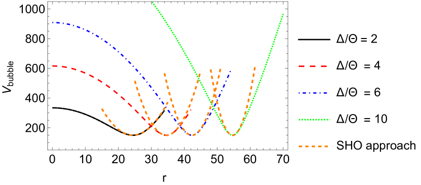
(a)

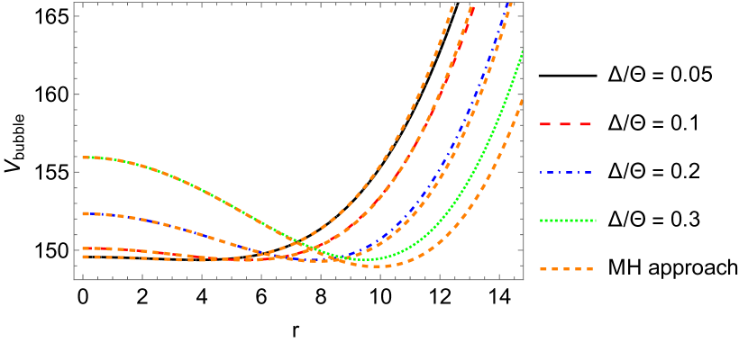
(b)

Figure 1: Comparison between bubble trap potentials, given by Eq. (2), with $\Theta=75$ and several values of $\Delta$. We employed two approximations: (a) the shifted harmonic oscillator, Eq. (4), and (b) the Mexican hat, Eq. (5). The latter is valid for small values of the detuning parameter ($\Delta/\Theta\ll 1$).

Mexican hat.— We explored another limit of Eq. (3) considering the expansion of $r\rightarrow 0$,

$$\begin{split}{V}_{\textrm{Bubble}}(r)=&\frac{r_{\rm min}^{2}\sqrt{1+\sigma^{2}}}{2}-\frac{1}{2\sqrt{1+\sigma^{2}}}r^{2}\\ +&\frac{\sigma^{2}}{4r_{\rm min}^{2}(1+\sigma^{2})^{3/2}}r^{4}+O(r^{6}).\end{split}$$ (5)

This approximation is reasonable if $\sigma>1$, i.e., for a thick bubble. Figure 1b shows that the MH approximation is in excellent agreement with the bubble trap for $1/\sigma=0.05$, but gets progressively worst for thinner shells.

II.2 Hamiltonian in the rotating frame

In the previous section, we were treating a spherically-shaped bubble trap. However, this work aims to explore ring trap configurations under rotation. A ring trap can be produced by superposing a bubble trap with a vertical optical trap. That gives us a widely tunable trap, with the radius of the ring varying from $10\mu$m to $100\mu$m, and with a fixed coordinate $z_{0}$ in the vertical direction for the trapped atoms de Goër de Herve et al. (2021). It is straightforward to derive the SHO and MH potential profiles in 2D from Eqs. (4) and (5), respectively, after the replacement $r=\sqrt{\rho^{2}+z_{0}^{2}}$, where $\rho$ is the usual polar coordinate. For the SHO case, we have to consider additionally $\rho\gg z_{0}$, which is a very reasonable experimental condition Garraway and Perrin (2016); de Goër de Herve et al. (2021).

An alternative way of generating a ring configuration is dynamically, with the gas initially pooled at the bottom of a bubble trap due to the action of gravity. Then, suppose we increase the rotation rate. In that case, centrifugal effects propel the gas over the isomagnetic surface. Eventually, the potential minimum, considering gravity and rotation, assumes some non-zero value in the gravity direction. The disposition of the gas is then one of a dynamical ring. However, the precise parameterization of the radius of the ring and the minimum height of the potential as a function of the angular speed is a challenging problem Guo et al. (2020).

There are two main experimental methods for rotating the atoms. One consists in deforming the trap and rotating the deformation Jin et al. (1996); Mewes et al. (1996). The other is based on a blue-detuned laser to stir the atoms in the ring trap Marzlin et al. (1997); Dum et al. (1998). The rotating frame Hamiltonian $H^{\prime}$ is related to the one in the laboratory frame $H$ by

$$H^{{}^{\prime}} = H-\mathbf{\Omega}\cdot\mathbf{L},$$

$$H^{{}^{\prime}} = \sum_{i=1}^{N}\left[\frac{\mathbf{p}_{i}^{2}}{2}+V(\mathbf{r}_{i})\right]+\frac{G_{2D}}{N}\sum_{i<j}\delta(\mathbf{r}_{i}-\mathbf{r}_{j})$$ (6)

$$- \sum_{i=1}^{N}\mathbf{\Omega}\cdot\left(\mathbf{r}_{i}\times\mathbf{p}_{i}\right),$$

where the usual polar coordinates give the two-dimensional position of the atoms, ${\mathbf{r}}_{i}\equiv(\rho_{i},\varphi_{i})$, and $N$ is the total number of particles. In Eq. (II.2) we also introduced the angular velocity $\mathbf{\Omega}$ and the dimensionless 2D coupling constant $G_{2D}\equiv N\tilde{g}_{2D}/(\hbar\tilde{\omega}_{0}\tilde{\ell}_{0}^{2})$, where $\tilde{g}_{2D}$ characterizes the inter-atomic interactions. The 2D interaction strength is related to its three-dimensional (3D) counterpart by

$$\tilde{g}_{2D}=\frac{\tilde{g}_{3D}}{\sqrt{2\pi}\tilde{Z}},$$ (7)

where $\tilde{Z}$ is associated with the length scale of the optical-trap confinement in the $z$-direction.

III Phase Diagram

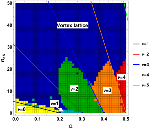
(a)

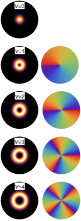
(b)

Figure 2: (a) Phase diagram of the Mexican hat potential, Eq. (11), with $\lambda=0.1$. The colors represent the region of each macrovortex configuration, i.e., the pure states, with increasing values of vorticity (starting from the left side, with $\nu$ going from $0$ to $4$) as predicted by variational calculations. The lines represent first-order phase transitions calculated with perturbation theory, Eq. (13). (b) Phase and density profiles of the macrovortex states. The first profile shows a zero vorticity configuration represented in the phase diagram by the area below the solid black line.

To characterize the phase diagram of the system, we applied the variational technique as described in the following. Provided the interaction parameter $G_{2D}$ is sufficiently small, we can consider the eigenstates of the harmonic potential without radial excitations, and angular momentum $m$ as our unperturbed states $|\Phi_{m}\rangle$ Jackson and Kavoulakis (2004). Therefore, the condensate wave function can be represented by the variational ansatz

$$|\psi\rangle=\sum_{m=0}^{N_{\rm max}}c_{m}|\Phi_{m}\rangle,$$ (8)

with

$$\langle\bm{r}|\Phi_{m}\rangle=\frac{\rho^{m}e^{im\varphi}}{\sqrt{\pi m!}}e^{-\frac{\rho^{2}}{2}},$$ (9)

and

$$\sum_{m=0}^{N_{\rm max}}|c_{m}|^{2}=1.$$ (10)

These functions are the basis of the functional space over which we minimize the energy.

We begin by choosing a value for the rotation speed $\Omega$ and the interaction parameter $G_{2D}$. We find numerically the set of coefficients which minimize the energy, given by the expected value of Eq. (II.2). It is possible to classify this $(\Omega,G_{2D})$ pair as a macrovortex if $|c_{m}|^{2}\approx 1$ (within a $10^{-3}$ tolerance) for only one $m$ or as a vortex lattice if there are multiple coefficients contributing to the wave function. Then, the procedure is repeated for several values of $(\Omega,G_{2D})$.

III.1 Mexican hat

III.1.1 First-order transition

For the Mexican hat, we have Eq. (II.2) with

$$V(\rho)=\frac{1}{2}(-\rho^{2}+\lambda\rho^{4}).$$ (11)

To use the eigenfunctions given by Eq. (9) we also require $\lambda\ll 1$. In Fig. 2a, we present our results for $\lambda=0.1$. Hereafter we denote the macrovortex charge by $\nu$. In the parameter space explored in this work, $0.0\leqslant\Omega\leqslant 0.5$ and $0\leqslant G_{2D}\leqslant 50$, we observed macrovortices with charge varying from $\nu=0$ up to 4. The density profiles and respective phases of the wave functions in each of these regions are illustrated in Fig. 2b. In addition, we observed an upper (blue) region not described by one single coefficient $c_{m}$, signalling the appearance of vortex lattices.

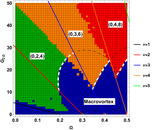
(a)

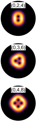
(b)

Figure 3: (a) Phase diagram of the Mexican hat potential, Eq. (11), with $\lambda=0.1$. The blue region collects the zero vorticity regime plus the macrovortex regions, whereas the other colored regions correspond to different vortex lattices indexed by $(0,m_{0},2m_{0})$. The solid lines represent the perturbative prediction for the first-order transition between the macrovortex regions. The dashed curves delimit the stability region of each macrovortex configuration, with the highlighted white thick dashed curves representing the second-order transition from a macrovortex to a vortex lattice phase. Above (below) the white curves, the system is expected to be in a lattice (macrovortex) configuration. (b) Vortex lattice density profiles.

A few words about the parameter space we chose to employ in this work are in order. The confinement in the $z$-direction must be strong enough so that the relevant dynamics takes place only in the $xy$-plane. A length scale $Z=0.1$ is one order of magnitude smaller than the harmonic oscillator length, thus accomplishing this goal. The interaction strength is given by $G_{2D}=\sqrt{8\pi}N{a}_{s}/Z$. Thus, even for the maximum value of $G_{2D}=50$ that we considered, we have $Na_{s}\sim 1$. Hence, we are far from the Thomas-Fermi regime, and the ansatz of Eq. (8) is valid.

Next, we wanted to compare our numerical variational results with perturbation theory predictions. We calculated the expectation value of $H^{{}^{\prime}}$ in the pure macrovortex states $|\Phi_{\nu}\rangle$ by using first-order perturbation theory to consider the interaction energy per particle and the anharmonicity contribution of the trap Jackson et al. (2004). Then we compared the energy of states $\nu$ and $\nu+1$ to extract the macrovortex phase boundaries. This gives us an analytical expression for the critical frequency $\Omega$, which delimits the transition between macrovortices states in the $G_{2D}\times\Omega$ phase diagram.

The energy $E_{\nu}$ of a pure macrovortex state $|\Phi_{\nu}\rangle$ is given by

$$E_{\nu} = \langle\Phi_{\nu}|H^{{}^{\prime}}|\Phi_{\nu}\rangle$$ (12)

$$= \frac{1}{2}\lambda\;(1+\nu)(2+\nu)+\frac{G_{2D}}{4\pi}\frac{(2\nu)!}{2^{2\nu}(\nu!)^{2}}$$

$$- \nu\Omega.$$

Comparing the energies $E_{\nu}$ and $E_{\nu+1}$, we obtain the critical frequency for the macrovortex phase transition,

$$\Omega\left(G_{2D}\right)=\lambda\;(1+\nu)-\frac{G_{2D}}{2\pi}\frac{(2\nu-2)!}{2^{2\nu}(\nu-1)!\nu!}.$$ (13)

Equation (13) is a line in the $G_{2D}\times\Omega$ phase diagram, with the intercept proportional to the anharmonicity.

We included the first-order perturbation theory results, Eq. (13), as solid lines in Fig. 2a. The lines delimit reasonably well the transition between the different macrovortex configurations for small values of $G_{2D}$. However, as we increase the value of the interaction, perturbation theory no longer accurately predicts the contours of transitions.

III.1.2 Second-order transition

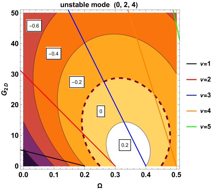
(a)

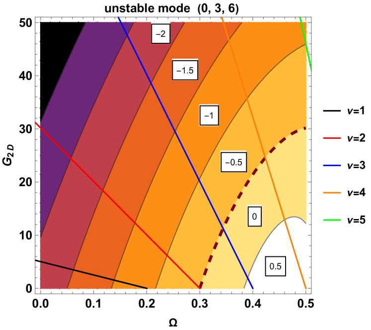
(b)

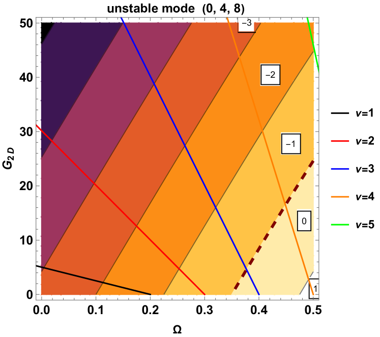
(c)

Figure 4: The figures show the value of the smallest eigenvalue of the stability matrix for the pure states $m_{0}=2,3,4$. The boundary of the positive region in each diagram corresponds to a second-order (continuous) phase transition from a macrovortex to vortex lattice regime. The solid lines are the results of first-order pertubation theory calculation, Eq. (13).

Let us consider the state of the system, starting from a macrovortex configuration, as we increase the interaction parameter $G_{2D}$. Initially, the state is characterized by some coefficient $|c_{m_{0}}|^{2}=1$ signalling unit occupation of the $m_{0}$ component in Eq. (8). As $G_{2D}$ increases, the occupation of $m_{0}$ slowly decreases and other states start to contribute to the total wave function. Eventually, the occupations of these states cease to be negligible and the system transitions from a pure macrovortex to a vortex lattice configuration.

Using the same variational results reported in the previous section, we now focus on the macrovortex to vortex lattice transitions. In Fig. 3a we indicate all the individual macrovortex regions ($\nu=0$ to 4) in blue. The other areas in the phase diagram correspond to vortex lattices. The classification of each of the lattice regions is given by a triple of numbers $(m_{1},m_{0},m_{2})$, which label the most occupied states, with $|c_{m_{0}}|^{2}+|c_{m_{1}}|^{2}+|c_{m_{2}}|^{2}\approx 1$ (within a $10^{-3}$ tolerance) and $|c_{m_{0}}|^{2}>|c_{m_{1}}|^{2},|c_{m_{2}}|^{2}$. For completeness, we keep the solid lines corresponding to Eq. (13) that would represent the boundaries of the macrovortex regions. In Fig. 3b, we show the density profiles of the vortex lattices.

The transition from the macrovortex state to the lattice configuration formed by singly-charged vortices occurs for sufficiently high interaction parameter values, which leave the macrovortex configuration energetically unstable. Analyzing the coefficients $c_{m}$, we also conclude that the most likely lattice mode for the decay of the macrovortex has the $(0,m_{0},2m_{0})$ combination of coefficients. This indicates that this mode is the most unstable one, which we confirmed by performing a stability analysis which we now describe.

We constructed a stability matrix formed by the derivative of the energy with respect to the coefficients of the system close to the transition Jackson et al. (2004). Suppose the system is stable in a macrovortex configuration characterized by angular momentum $m_{0}$. In that case, the energy derivative with respect to all $c_{m}$ must vanish, and the eigenvalues must be positive. The total energy is given by

$$E =\langle\psi(\mathbf{r})|H^{{}^{\prime}}|\psi(\mathbf{r})\rangle$$ (14)

$$=\frac{1}{S}\sum_{m}c_{m}^{2}\epsilon_{m}$$

$$+\frac{1}{S^{2}}\sum_{m,n,l,k}c_{m}c_{n}c_{l}c_{k}\langle m,n|V_{\rm int}|l,k\rangle\;\delta_{m+n,l+k},$$

where $\epsilon_{m}\equiv\lambda(m+1)(m+2)/2-m\Omega$ corresponds to the energy of a particle in the absence of interaction, $S\equiv\sum_{m}|c_{m}|^{2}$, and $V_{\rm int}\equiv(G_{2D}/N)\sum_{i<j}^{N}\delta(\mathbf{r}_{i}-\mathbf{r}_{j})$ is the interaction term. Its matrix elements are

$$\langle m,n|V_{\rm int}|l,k\rangle$$

$$=\int d^{2}\bm{r}\int d^{2}\bm{r^{\prime}}\Phi_{m}^{*}(\bm{r})\Phi_{n}^{*}(\bm{r^{\prime}})V_{\rm int}(\bm{r}-\bm{r^{\prime}})\Phi_{l}(\bm{r^{\prime}})\Phi_{k}(\bm{r})$$

$$=\frac{G_{2D}}{4\pi}\frac{(m+n)!}{2^{m+n}\sqrt{m!n!l!k!}}.$$ (15)

Note that $\partial E/\partial c_{m}=0$ when $c_{m_{0}}\to 1$ and $c_{m}\to 0$ for $m\neq m_{0}$, as required.

Since the coefficients are small, we need only to keep terms that are at most bilinear in $c_{m}$ for $m\neq 0$ in the interaction term. Because of the Kronecker delta, only the terms proportional to $\langle m_{i}m_{0}|V_{\rm int}|m_{i}m_{0}\rangle$ and $\langle m_{0}m_{0}|V_{\rm int}|m_{1}m_{2}\rangle$ need to be retained in the sum, the latter being the only off-diagonal element in the matrix.

The $m_{1}$ and $m_{2}$ numbers characterize the two relevant states at the transition, and the elements of the stability matrix corresponding to the state $m_{0}$ are related to the second derivative of the energy with respect to $m_{1}$ and $m_{2}$,

$$\frac{\partial^{2}E^{(2)}}{\partial{c_{m_{1}}}\partial{c_{m_{2}}}}=4c_{0}^{2}\langle m_{1}m_{2}|V_{\rm int}|m_{0}m_{0}\rangle\;\delta_{m_{1}+m_{2},2m_{0}},$$ (16)

and

$$\frac{\partial^{2}E^{(2)}}{\partial^{2}{c_{m_{i}}}} = 2\epsilon_{m_{i}}+8c_{0}^{2}\langle m_{i}m_{0}|V_{\rm int}|m_{i}m_{0}\rangle+$$ (17)

$$+ 4c_{0}^{2}\langle m_{0}m_{0}|V_{\rm int}|m_{0}m_{0}\rangle$$

$$= 2(\epsilon_{m_{i}}-\epsilon_{0})+8c_{0}^{2}\langle m_{i}m_{0}|V_{\rm int}|m_{i}m_{0}\rangle$$

$$- 4c_{0}^{2}\langle m_{0}m_{0}|V_{\rm int}|m_{0}m_{0}\rangle.$$

In Eq. (17) we used the identity $8c_{0}^{2}\langle m_{0}m_{0}|V_{\rm int}|m_{0}m_{0}\rangle=-2\epsilon_{0}$, which can be derived from the fact that $c_{m}=c_{m_{0}}$ is an energy minimum (${\partial E}/{\partial c_{m_{0}}}=0$). After choosing a value for the pure state $m_{0}$ and two values $m_{1}$ and $m_{2}$, we construct a $2\times 2$ matrix, with the diagonal values given by Eq. (17) and the off-diagonal values given by Eq. (16). This matrix is then diagonalized, and the resulting eigenvalues are used to analyze the stability of the pure state $m_{0}$. One of the eigenvalues is always positive, making the smallest eigenvalue the relevant one to investigate the stability.

The instability of the pure mode $m_{0}$ towards the decay to the lattice mode $(m_{1},m_{0},m_{2})$ is illustrated in Fig. 4 for the different types of lattices observed in the variational results, namely (0,2,4), (0,3,6), and (0,4,8). The figures represent the smallest eigenvalue of the stability matrix of the state $m_{0}$. The boundaries in the $G_{2D}\times\Omega$ diagram where this eigenvalue becomes negative represent the transition to a lattice configuration, which we highlight with a dashed curve.

Although the contour where the smallest eigenvalue changes signs intersects regions with different macrovortex charges $\nu$, a transition to a vortex lattice is only physically sensible if $\nu=m_{0}$. For example, in Fig. 4a, where $m_{0}=2$, it is the portion of the dashed curve between the lines corresponding to $\nu=2$ (red) and $\nu=3$ (blue). Analogously, the same is valid for $\nu=3$ and $\nu=4$ (orange) in Fig. 4b, and $\nu=4$ and $\nu=5$ (green) in Fig. 4c.

Furthermore, the instability to decay to the lattice mode is more significant as the negative eigenvalue is larger in magnitude. This explains the competition between lattice modes, which defines the boundaries of the colored regions in the diagram of Fig. 3.

To make comparisons easier, we included the dashed curves of Fig. 4 in the $G_{2D}\times\Omega$ phase diagram, Fig. 3. The regions where a macrovortex to vortex lattice transition is expected, as discussed above, are highlighted as white dashed curves. We see they reasonably delimit the beginning of the vortex lattice regions obtained with the variational technique.

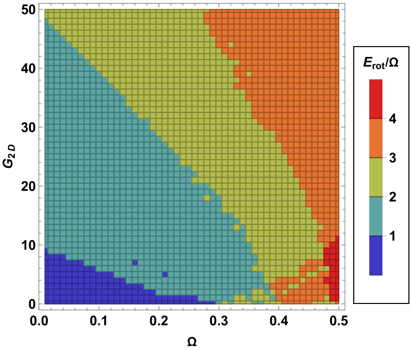
(a)

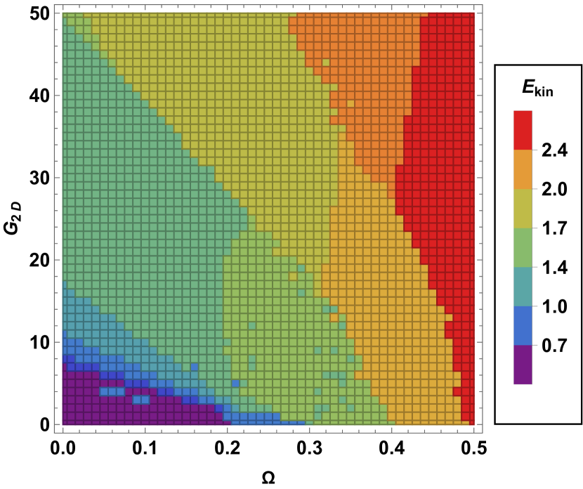
(b)

Figure 5: Partial energy diagrams for the Mexican hat potential, Eq. (11), with $\lambda=0.1$, where signatures of the first- and second-order phase transitions can be seen. (a) The rotational energy shows the first-order boundaries, corresponding to transitions between macrovortices with different charges. (b) The kinetic energy signalizes the second-order (continuous) macrovortex to vortex lattice transitions.

The wave function, Eq. (8), can also be used to compute the partial energies of the system,

$$E_{kin} = \frac{1}{2}\sum_{i}\langle\psi\left|p_{i}^{2}\right|\psi\rangle,$$

$$E_{trap} = \sum_{i}\langle\psi\left|V(\bm{r}_{i})\right|\psi\rangle,$$

$$E_{int} = \frac{G_{2D}}{N}\sum_{i<j}\langle\psi\left|\delta(\bm{r}_{i}-\bm{r}_{j})\right|\psi\rangle,$$

$$E_{rot} = \sum_{i}\langle\psi\left|\bm{\Omega}\cdot\bm{L}_{i}\right|\psi\rangle,$$ (18)

the kinetic, trapping potential, interaction, and rotation energies, respectively. They are related to the total energy $E$ through

$$E=E_{kin}+E_{trap}+E_{int}-E_{rot}.$$ (19)

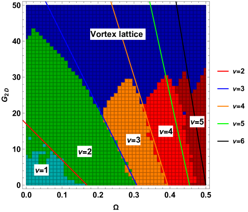
(a)

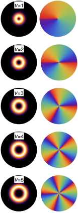
(b)

Figure 6: (a) Phase diagram of the SHO potential, Eq. (20), with $\rho_{0}=2.5$. The blue color represents the vortex lattice region, while the other colors indicate the region of each macrovortex configuration with increasing values of vorticity, with $\nu$ going from $1$ to $5$. The lines denote the first-order phase transition calculated through perturbation theory, Eq. (22), which approximately delimited each macrovortex region. In contrast to Figure 2, the SHO potential appears to act as a pinning potential stabilizing the macrovortices, as these states occupy a larger area of the phase diagram when compared to the MH potential. (b) Phase and density profiles of the corresponding macrovortex states.

The phase diagram analysis of these partial energies also gives insights into the transitions between different macrovortex states and vortex lattices. This can be seen in Fig. 5a, which illustrates the quantized values of the rotational energy normalized by the frequency $\Omega$. In Fig. 5b, on the other hand, the variation in the kinetic energy appears to signal the second-order transitions. It decreases abruptly when we have the decay to a vortex lattice, which is more energetically favorable for larger values of the interaction parameter $G_{2D}$. We conclude that, in this trap, a multiply-charged vortex can be energetically stable for sufficiently weak interactions. However, as the interaction strength increases, it eventually becomes energetically favorable for the system to spread its angular momentum to additional states, and multiply-quantized vortex states break into singly-charged vortices. We found that the diagrams for $E_{trap}$ and $E_{int}$ did not yield any additional information about the transitions.

III.2 Shifted harmonic oscillator

For the SHO potential, we have Eq. (II.2) with

$$V(\rho)=\frac{1}{2}(\rho-\rho_{0})^{2}.$$ (20)

Besides the change in the trapping potential, the variational numerical procedure is the same as the one described in Sec. III.1. We employed the same range of $\Omega$ and $G_{2D}$ values as in the MH case to allow for direct comparison between the two traps.

Figure 6a shows the phase diagram concerning the macrovortices. We observe that the macrovortex region fills a larger area of the phase diagram for the SHO when compared to the MH case. This reflects the fact that the SHO potential works as a stabilizer “pinning” potential of the macrovortex configuration, making it more stable against a continuous transition to the lattice phase if compared to the MH trap. Furthermore, we see that, for the same $\Omega$ used in the case of MH, we obtained higher values for the charge $\nu$ of the macrovortex. Thus, we conclude that with the shifted harmonic oscillator trap, we could transfer angular momentum more efficiently to the superfluid, reaching higher vorticities with lower $\Omega$ values and having a more stable macrovortex configuration to be studied experimentally. In Fig. 6b, we reproduce the density and phase profiles of the observed macrovortices.

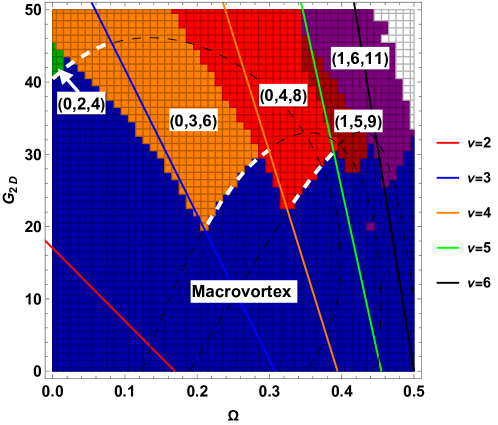
(a)

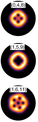
(b)

Figure 7: (a) Phase diagram for the shifted harmonic oscillator potential, Eq. (20), with $\rho_{0}=2.5$. The blue color represents the macrovortex region, and the white color denotes a region where the numerical procedure is unstable, signalling its limit for large values of $\Omega$ and $G_{2D}$. The other colors define regions corresponding to different lattice regimes, indexed by the $(m_{1},m_{0},m_{2})$ triples. As in the diagram of Fig. 3a, the highlighted white thick dashed line represents the second-order transition from the macrovortex to the vortex lattice phase. (b) Corresponding vortex lattice density profiles. The (0,2,4) and (0,3,6) density plots are the same as those depicted in Fig. 3b.

To accurately describe the regions with large values of $\Omega$ and $G_{2D}$, we had to carefully check the number of terms used in the variational calculation, Eq. (8). We employed $N_{\rm max}\sim 3\nu$ in the case of macrovortices and $N_{\rm max}\sim 3m_{0}$ for vortex lattices. For a macrovortex, $N_{\rm max}=\nu$ would suffice, but for a vortex lattice described by the triple $(m_{1},m_{0},m_{2})$, we need $N_{\rm max}$ to be at least the maximum between these three values. For a fixed value of $m_{0}$, the $m_{1}+m_{2}=2m_{0}$ constrain makes the triples of the form $(0,m_{0},2m_{0})$ the more demanding ones (for $m_{1}\neq 0$ then $m_{2}<2m_{0}$ and fewer coefficients are required). Hence we employed $N_{\rm max}\sim 3\nu$ or $\sim 3m_{0}$ to have a margin of safety and also because, given a $(\Omega,G_{2D})$ pair, we do not know a priori what the vortex configuration is.

Using first-order perturbation theory, we determined the energy for a pure macrovortex state characterized by a single number $\nu$,

$$E_{\nu}=1+\nu+\frac{\rho_{0}^{2}}{2}-\frac{\rho_{0}\sqrt{\pi}}{2}\frac{(2\nu+1)!}{2^{2\nu}(\nu!)^{2}}+\frac{G_{2D}}{4\pi}\frac{(2\nu)!}{2^{2\nu}(\nu!)^{2}}-\nu\Omega.$$ (21)

Equating the energies $E_{\nu}$ and $E_{\nu+1}$, we obtain the critical frequency for the macrovortex phase transition,

$$\Omega\left(G_{2D}\right)=1-\frac{\rho_{0}\sqrt{\pi}}{2}\frac{(2\nu)!}{2^{2\nu}(\nu!)^{2}}-\frac{G_{2D}}{2\pi}\frac{(2\nu-2)!}{2^{2\nu}(\nu-1)!\nu!}.$$ (22)

We included the lines given by Eq. (22) in Fig. 6a. We observe a qualitative agreement for $\nu<4$, but for higher values of the macrovortex charge, the regions are not well-described by first-order perturbation theory.

The absence of the $\nu=0$ mode is a consequence of Eq. (21), which shows that for any value of $\Omega$, $E_{0}$ is always larger than $E_{1}$. This equation was derived using an ansatz where a hole cannot be present in the center of the condensate for zero angular momentum, so it is natural to expect the absence of a zero angular momentum region. Since our interest is in rotating condensates, this region should not affect our analysis.

In Fig. 7a we focus on the vortex lattices. Because of angular momentum conservation, as in the case of MH, we have the constraint $m_{1}+m_{2}=2m_{0}$, with $m_{0}$ having majority occupation and $|c_{m_{0}}|^{2}+|c_{m_{1}}|^{2}+|c_{m_{2}}|^{2}\approx 1$ (within a $10^{-3}$ tolerance). The blue color characterizes the macrovortices region and each other color indicates a vortex lattice, indexed by the $(m_{1},m_{0},m_{2})$ triples. The correspondent lattices density profiles are given in Fig. 7b. The analysis based on the stability matrices calculated for each pure state mode, as shown in Fig. 8, accurately predicted the boundary between the macrovortex and lattice regions.

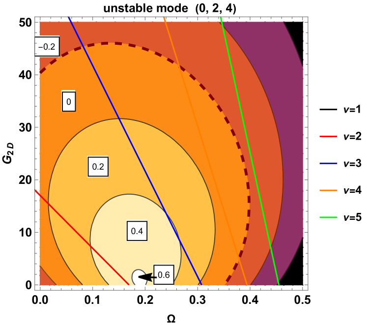
(a)

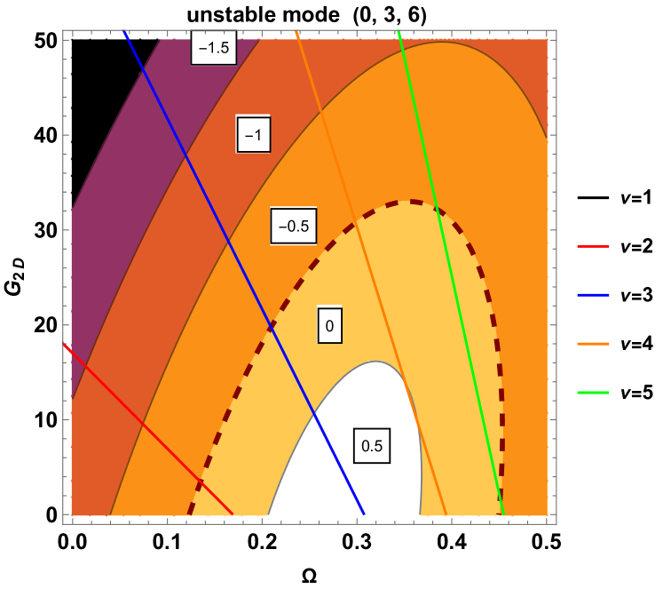
(b)

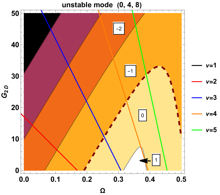
(c)

Figure 8: The figures indicate the value of the smallest eigenvalue of the stability matrix for the pure macrovortex states $m_{0}=2,3,4$. The boundary of the positive region in each diagram corresponds to a second-order (continuous) phase transition from macrovortex to vortex lattice regime.

In the MH case, we only observed lattices of the $(0,m_{0},2m_{0})$ type. For the SHO trapping potential, we notice the presence of the vortex lattices $(1,5,9)$ and $(1,6,11)$, which have a central vortex of charge one.

For large values of $\Omega$ and $G_{2D}$, the white region in Fig. 7a, we observed a non-negligible value for more than three $c_{m}$ coefficients. Increasing the number of $N_{\rm max}$ terms used in the variational calculation, Eq. (8), led to numerical instabilities. This indicates the limitation of the procedure we adopted, as it is, for large values of $\Omega$ and $G_{2D}$. In future studies, we intend to investigate if the parameter space can be constrained to improve the variational procedure, if a different ansatz is necessary for this region, or if more than three $c_{m}$ coefficients truly characterize the phase.

Finally, in Fig. 9, we present the analysis of the partial energy diagrams. As in the case of the MH potential, the rotational energy normalized by $\Omega$ shows the quantized values of $\nu$ related to the phases of macrovortices. On the other hand, the kinetic energy diagram shows a sudden decrease in energy when crossing the boundary from a macrovortex to a vortex lattice configuration.

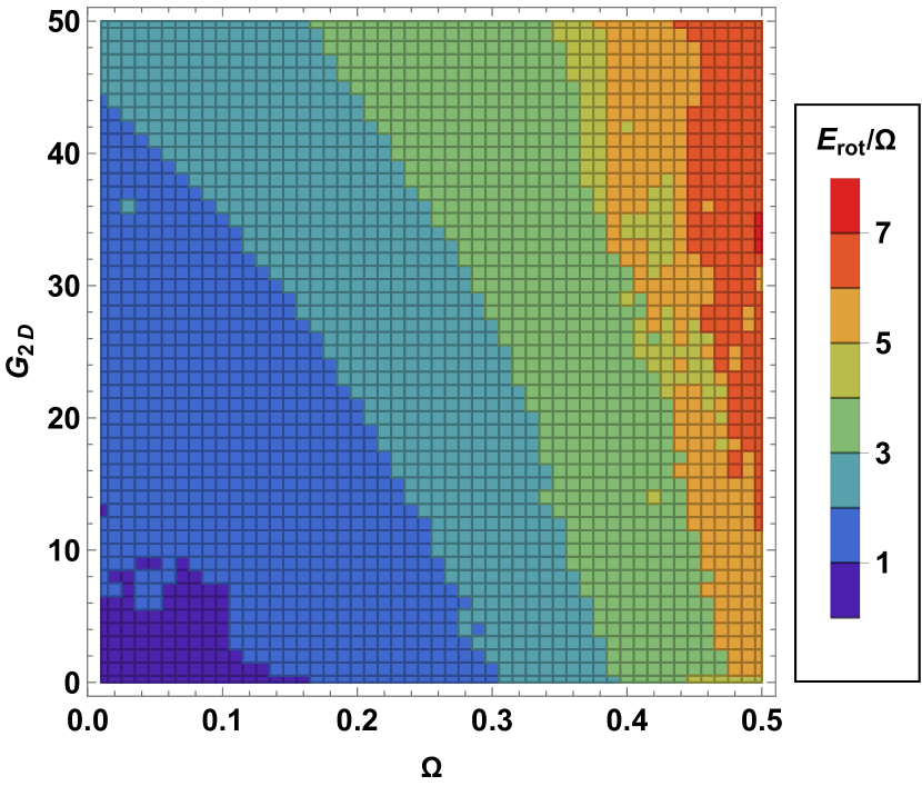
(a)

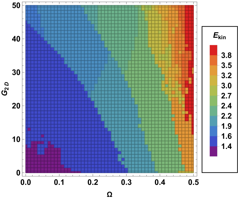
(b)

Figure 9: Partial energy diagrams for the SHO potential, Eq. (20), with $\rho_{0}=2.5$. (a) The rotational energy indicates the first-order phase transitions between macrovortices. (b) In the kinetic energy, it is possible to see the second-order (continuous) transitions from macrovortices to vortex lattices.

The energy analysis is explored further in the next section, where we show how the frequencies of the collective modes change when the system evolves from a macrovortex to a singly-charged vortex lattice configuration.

IV Collective modes and Sum Rules

Consider an arbitrary physical operator $\hat{F}$ exciting the system from its ground state $|0\rangle$ to an excited state. The response of the system ground state to the action of the operator $\hat{F}$ is characterized by the strength function,

$$S(\omega)=\sum_{n>0}|\langle n|\hat{F}|0\rangle|^{2}\delta(\omega-\omega_{n}),$$ (23)

where $\omega_{n}=E_{n}-E_{0}$, with the Hamiltonian of the system satisfying $\hat{H}|n\rangle=E_{n}|n\rangle$. Determining $S(\omega)$ can be difficult since it involves the calculation of all the eigenstates of $\hat{H}$. The sum-rule technique provides a useful alternative to the explicit evaluation of $S(\omega)$. It is based on the determination of the moments $m_{p}$ of the strength function,

$$m_{p}=\int_{0}^{\infty}S(\omega)\omega^{p}d\omega=\sum_{n>0}|\langle n|\hat{F}|0\rangle|^{2}\omega_{n}^{p},$$ (24)

which can be rewritten as mean values on the ground state of the system. For operators $\hat{F}$ such that $\langle 0|\hat{F}|0\rangle=0$, and $p\geqslant 0$, one has

$$m_{p} =\sum_{n}\langle 0|\hat{F}^{\dagger}|n\rangle\langle n|\hat{F}|0\rangle(E_{n}-E_{0})^{p}$$ (25)

$$=\langle 0|\hat{F}^{\dagger}(\hat{H}-E_{0})^{p}\hat{F}|0\rangle,$$

where we used the completeness relation $\sum_{n}|n\rangle\langle n|=\hat{I}$. The sum-rule approach is particularly useful when a few moments can characterize the strength function. It is straightforward to check that the moments in Eq. (25) with $p>0$ can be expressed through commutators and anti-commutators involving the excitation operator and the Hamiltonian of the system $\hat{H}$ Lipparini and Stringari (1989).

To investigate the collective modes of a system described by $\hat{H}$, we consider a complete set of exact eigenstates $\{|n\rangle\}$ and eigenvalues $\{E_{n}\}$ of this Hamiltonian, with $E_{0}\leqslant E_{1}\leqslant E_{2}...$, and also an excitation operator of the system $\hat{F}$. An upper bound $\hbar\omega^{\rm upper}$ to the minimum excitation energy $\hbar\omega^{\rm min}=E_{1}-E_{0}$ of the states excited by $\hat{F}$ is given by

$$\hbar\omega^{\rm upper}\geqslant\sqrt{m_{3}/m_{1}}.$$ (26)

This follows from the definition of the moments in Eq. (24), from which we can show that

$$\frac{(\omega^{\rm upper})^{2}-(\omega^{\rm min})^{2}}{(\omega_{1}-\omega_{0})^{2}}+1 = \frac{\sum\limits_{n>0}|\langle n|\hat{F}|0\rangle|^{2}\frac{(\omega_{n}-\omega_{0})^{3}}{(\omega_{1}-\omega_{0})^{3}}}{\sum\limits_{n>0}|\langle n|\hat{F}|0\rangle|^{2}\frac{(\omega_{n}-\omega_{0})}{(\omega_{1}-\omega_{0})}}.$$

Since we have

$$\frac{(\omega_{n}-\omega_{0})}{(\omega_{1}-\omega_{0})}\geqslant 1,$$ (28)

we conclude that $\omega^{\rm upper}\geqslant\omega^{\rm min}$. The advantage of the sum-rule approach is that just the ground state is required to calculate the moments [see Eq. (25)] and then to find the strength function. If, in particular, the excitation operator $\hat{F}$ excites a single state and we have knowledge of the exact ground state, $\hbar\omega^{\rm upper}$ gives the exact excitation energy.

Before we introduce the collective modes, which are characterized by the symmetries of the chosen excitation operator $\hat{F}$, we need to generalize the definition of the moments for a non-Hermitian operator ($\hat{F}\neq\hat{F}^{\dagger}$). Calling $\hat{F}=F_{+}$ and $\hat{F}^{\dagger}=F_{-}$, we define

$$m_{p}^{\pm}=\int_{0}^{\infty}\;d\omega\left[S_{+}(\omega)\pm S_{-}(\omega)\right]\omega^{p},$$ (29)

with

$$S_{\pm}(\omega)=\sum_{n>0}|\langle n|F_{\pm}|0\rangle|^{2}\delta(\omega-\omega_{\pm}),$$ (30)

where $E_{\pm}$ corresponds to the energies of the modes that we want to determine. In terms of the previous definition given by Eq. (24), we have that $m_{p}^{\pm}=m_{p}(\hat{F})\pm m_{p}(\hat{F}^{\dagger})$. We will apply the general formula in Eq. (29) to deal with the quadrupole mode operator.

IV.1 Excitation Operator

We start by defining a general excitation operator using spherical coordinates and the spherical harmonics expansion. We note that these operators can be defined disregarding an overall multiplicative constant since the moments depend on ratios involving the operators both in the numerator and the denominator. The general form of the operator is

$$\hat{F}(n,\ell,m)\propto\sum_{j}r_{j}^{2n+\ell}Y_{\ell,m}(\theta_{j},\phi_{j}),$$ (31)

where $Y_{\ell,m}$ represents the spherical harmonics and the sum is taken over the particles of the system. The excitation with $n=1$ and $\ell=m=0$ is called the monopole mode, and the corresponding operator is

$$\hat{F}_{M}\equiv\hat{F}(1,0,0)\propto\sum_{j}r_{j}^{2}=\sum_{j}(x_{j}^{2}+y_{j}^{2}+z_{j}^{2}).$$ (32)

The excitations with $n=0$ and $\ell=2$ are identified with the quadrupole modes, which are classified into five types depending on the value of $m$,

$$\hat{F}_{Q} \equiv \hat{F}(0,2,m)\propto\sum_{j}r_{j}^{2}Y_{2,m}(\theta_{j},\phi_{j})$$ (33)

$$\propto \begin{cases}\sum\limits_{j}(x_{j}\pm iy_{j})^{2},&\text{for }m=\pm 2,\\ \sum\limits_{j}(x_{j}\pm iy_{j})z_{j},&\text{for }m=\pm 1,\\ \sum\limits_{j}(x_{j}^{2}+y_{j}^{2}-2z_{j}^{2}),&\text{for }m=0.\end{cases}$$

IV.2 Monopole mode

Previously, we considered the upper bound of the lowest energy excited by an operator $\hat{F}$. The equality in Eq. (26) holds whenever $\hat{F}$ excites one single mode. This section studies the breathing oscillation expected to be excited by the monopole operator. We extracted the frequency of the lowest excited mode from

$$\hbar\omega=\sqrt{m_{3}/m_{1}}.$$ (34)

The explicit calculation of the moments $m_{p}$ for $p>0$ can be carried out in terms of commutators between the excitation operator and the Hamiltonian of the system evaluated on the ground state Lipparini and Stringari (1989),

$$m_{1}=\frac{1}{2}\langle 0|[\hat{F},[\hat{H},\hat{F}]]|0\rangle,$$ (35)

and

$$m_{3}=\frac{1}{2}\langle 0|[[\hat{F},\hat{H}],[\hat{H},[\hat{H},\hat{F}]]]|0\rangle.$$ (36)

In the following, we considered the perturbation given by the 2D version of Eq. (32) and the rotating frame many-body Hamiltonian, Eq. (II.2).

For the Mexican hat trapping potential with anharmonicity $\lambda$ we obtain the frequency

$$\omega_{{M}}^{MH}=\sqrt{2\frac{E_{kin}}{E_{ho}}-2+2\frac{E_{int}}{E_{ho}}+8\lambda\frac{\langle\rho^{4}\rangle}{\langle\rho^{2}\rangle}}.$$ (37)

Using the Virial theorem (see appendix A), it can be rewritten as

$$\omega_{{M}}^{MH}=\sqrt{2+6\frac{E_{kin}}{E_{ho}}+6\frac{E_{int}}{E_{ho}}}.$$ (38)

Repeating the same calculation for the shifted harmonic oscillator trap with radius $\rho_{0}$ yields

$$\omega_{{M}}^{\rm SHO}=\sqrt{2\frac{E_{kin}}{E_{ho}}+2+2\frac{E_{int}}{E_{ho}}-\rho_{0}\frac{\langle\rho\rangle}{\langle\rho^{2}\rangle}},$$ (39)

which is equivalent to

$$\omega_{{M}}^{\rm SHO}=\sqrt{1+3\frac{E_{kin}}{E_{ho}}+3\frac{E_{int}}{E_{ho}}}.$$ (40)

Equations (37)-(40) contain the kinetic and interaction energies given by the same expressions as in Eq. (III.1.2). The difference is that in Secs. III.1.2 and III.2, we used the variational wave function to compute the partial energies, but here we employed the ground state solution of the GPE. Equations (37)-(40) also feature $E_{ho}$, given by

$$E_{ho}=\frac{\langle\rho^{2}\rangle}{2}.$$

IV.3 Quadrupole mode

To calculate the quadrupole modes in a condensate with vortices, we have to include a larger number of modes and moments in the analysis. Importantly, a splitting in the quadrupole mode frequency is expected due to vortices in the condensate  Zambelli and Stringari (1998). This can be understood by noting that the average velocity flow associated with the collective oscillation can be either parallel or opposite to the vortex flow, depending on the sign of the angular momentum carried by the excitation, thus producing a shift in the collective mode frequency. Specifically, to deal with the frequency degenerescence in the sum rule, we used the two modes approach,

$$S_{\pm}(\omega)=\sigma^{\pm}\delta(\omega-\omega_{\pm}),$$ (41)

with $\sigma^{+}=\sigma^{-}=\sigma_{0}$ ($m_{0}^{-}=\sigma^{+}-\sigma^{-}=0$). We have, according to Eq.(29),

$$m_{1}^{+}=\sigma_{0}\left(\omega_{+}+\omega_{-}\right),$$ (42)

$$m_{-1}^{+}=\sigma_{0}\left(\frac{1}{\omega_{+}}+\frac{1}{\omega_{-}}\right)=\frac{m_{1}^{+}}{\omega_{+}\omega_{-}},$$ (46)

$$m_{2}^{-}=\sigma_{0}\left(\omega_{+}^{2}-\omega_{-}^{2}\right)=m_{1}^{+}\left(\omega_{+}-\omega_{-}\right),$$

$$m_{3}^{+}=\sigma_{0}\left(\omega_{+}^{3}+\omega_{-}^{3}\right)=m_{1}^{+}\left(\omega_{+}^{2}-\omega_{+}\omega_{-}+\omega_{-}^{2}\right),$$

$$m_{4}^{-}=\sigma_{0}\left(\omega_{+}^{4}-\omega_{-}^{4}\right)=m_{2}^{-}\left(\omega_{+}^{2}+\omega_{-}^{2}\right).$$

Using Eqs. (42) and (46) yields

$$\omega_{+}-\omega_{-}=\frac{m_{2}^{-}}{m_{1}^{+}},$$

$$\omega_{+}\omega_{-}=\frac{m_{1}^{+}}{m_{-1}^{+}},$$ (47)

and solving for the energies,

$$\omega_{\pm}=\frac{1}{2}\left[\sqrt{\left(\frac{m_{2}^{-}}{m_{1}^{+}}\right)^{2}+4\frac{m_{1}^{+}}{m_{-1}^{+}}}\mp\frac{m_{2}^{-}}{m_{1}^{+}}\right].$$ (48)

Equations (46) and (46) provide the identity

$$\frac{m_{3}^{+}}{m_{1}^{+}}=\frac{m_{4}^{-}}{m_{2}^{-}}-\frac{m_{1}^{+}}{m_{-1}^{+}}.$$ (49)

Finally, to avoid the calculation of the $m_{-1}$ moments which are intricate, we rewrite Eq. (IV.3) using the identity above,

$$\omega_{\pm}=\frac{1}{2}\left[\sqrt{\left(\frac{m_{2}^{-}}{m_{1}^{+}}\right)^{2}+4\left(\frac{m_{4}^{-}}{m_{2}^{-}}-\frac{m_{3}^{+}}{m_{1}^{+}}\right)}\mp\frac{m_{2}^{-}}{m_{1}^{+}}\right].$$ (50)

As we will see afterwards, when we have the annular structure of the condensate, both the low- ($\omega_{-}$) and high-lying ($\omega_{+}$) energy branches acquire additional modes. These new modes, which have opposite azimuthal quantum numbers $m$, are very close in energy to the original $m=\pm 2$ modes. A full treatment of the 4-mode system would be very complicated. Instead, we assume that two doubly-degenerate energy levels are present in our analysis. Then, in the sum-rule calculation, we consider Eq. (29) with

$$\omega_{+}(\omega) = \sigma_{H}\delta(\omega-\omega_{H})+\sigma_{L}\delta(\omega-\omega_{L}),$$

$$\omega_{-}(\omega) = \sigma_{H}^{\dagger}\delta(\omega-\omega_{H})+\sigma_{L}^{\dagger}\delta(\omega-\omega_{L}).$$ (51)

That is, we assume the degenerescence between the energies of the higher ($\sigma_{H}$ and $\sigma_{H}^{\dagger}$) and lower ($\sigma_{L}$ and $\sigma_{L}^{\dagger}$) branches of the $m=\pm 2$ modes Cozzini (2006).

This gives us six equations,

$$m_{0}^{-}=\sigma_{H}+\sigma_{L}-\sigma_{H}^{\dagger}-\sigma_{L}^{\dagger}=0,$$ (52)

$$m_{-1}^{+}-=\frac{\sigma_{H}}{\omega_{H}}+\frac{\sigma_{L}}{\omega_{L}}+\frac{\sigma_{H}^{\dagger}}{\omega_{H}}+\frac{\sigma_{L}^{\dagger}}{\omega_{L}},$$ (53)

$$m_{1}^{+}=\sigma_{H}\omega_{H}+\sigma_{L}\omega_{L}+\sigma_{H}^{\dagger}\omega_{H}+\sigma_{L}^{\dagger}\omega_{L},$$ (54)

$$m_{2}^{-}=\sigma_{H}\omega_{H}^{2}+\sigma_{L}\omega_{L}^{2}-\sigma_{H}^{\dagger}\omega_{H}^{2}-\sigma_{L}^{\dagger}\omega_{L}^{2},$$ (55)

$$m_{3}^{+}=\sigma_{H}\omega_{H}^{3}+\sigma_{L}\omega_{L}^{3}+\sigma_{H}^{\dagger}\omega_{H}^{3}+\sigma_{L}^{\dagger}\omega_{L}^{3},$$ (56)

$$m_{4}^{-}=\sigma_{H}\omega_{H}^{4}+\sigma_{L}\omega_{L}^{4}-\sigma_{H}^{\dagger}\omega_{H}^{4}-\sigma_{L}^{\dagger}\omega_{L}^{4},$$ (57)

to be solved for six variables. We start with Eqs. (52)-(55) and solve for $\sigma_{H},\sigma_{H}^{\dagger}$, $\sigma_{L}$, and $\sigma_{L}^{\dagger}$. Then, we replace these solutions in Eqs. (56) and (57), which yields

$$\frac{m_{4}^{-}}{m_{2}^{-}}=\omega_{H}^{2}+\omega_{L}^{2},$$

$$\frac{m_{3}^{+}}{m_{1}^{+}}=\frac{m_{4}^{-}}{m_{2}^{-}}-\omega_{H}^{2}\omega_{L}^{2}\frac{m_{-1}^{+}}{m_{1}^{+}}.$$ (58)

Then, we find that

$$\omega_{H,L}^{4}-\left(\frac{m_{4}^{-}}{m_{2}^{-}}\right)\omega_{H,L}^{2}+\frac{m_{1}^{+}}{m_{-1}^{+}}\left(\frac{m_{4}^{-}}{m_{2}^{-}}-\frac{m_{3}^{+}}{m_{1}^{+}}\right)=0,$$ (59)

with the solutions,

$$\omega_{H,L}^{2}=\frac{1}{2}\left[\frac{m_{4}^{-}}{m_{2}^{-}}\pm\sqrt{\left(\frac{m_{4}^{-}}{m_{2}^{-}}\right)^{2}-4\frac{m_{1}^{+}}{m_{-1}}\left(\frac{m_{4}^{-}}{m_{2}^{-}}-\frac{m_{3}^{+}}{m_{1}^{+}}\right)}\right].$$ (60)

To calculate the two- and four-modes frequencies in Eqs. (50) and (60), we considered the non-Hermitian quadrupole perturbation operator as in Eq. (33),

$$F_{\pm}=\sum_{j=1}^{N}(x_{j}\pm iy_{j})^{2},$$ (61)

where $F_{+}=F_{-}^{\dagger}$. The details of the calculations of the modes are given in Appendix C.

IV.4 Comparison with numerical simulations

Finally, to complete our analysis of the collective modes, we considered numerical solutions of the Gross-Pitaevski equation,

$$i\frac{\partial\psi}{\partial t}=-\frac{1}{2}\nabla^{2}\psi+V\psi+G_{2D}|\psi|^{2}\psi-\bm{\Omega}\cdot\bm{L}\psi,$$ (62)

where $\nabla^{2}$ is the two-dimensional Laplacian operator. The propagation in imaginary time yields the ground state, while real time simulations can be employed to study the dynamics of the condensate. We modified the code developed in Ref. Kishor Kumar et al. (2019), which uses a Crank-Nicolson scheme to find the numerical wave function.

Our variational results obtained in Sec. III, for a given $\Omega$ and $G_{2D}$, were used as the initial conditions for imaginary time propagation. The resulting numerical ground state of the system is then used both for computing the average values described in Secs. IV.2 and IV.3 and for investigating the collective modes in real time propagation.

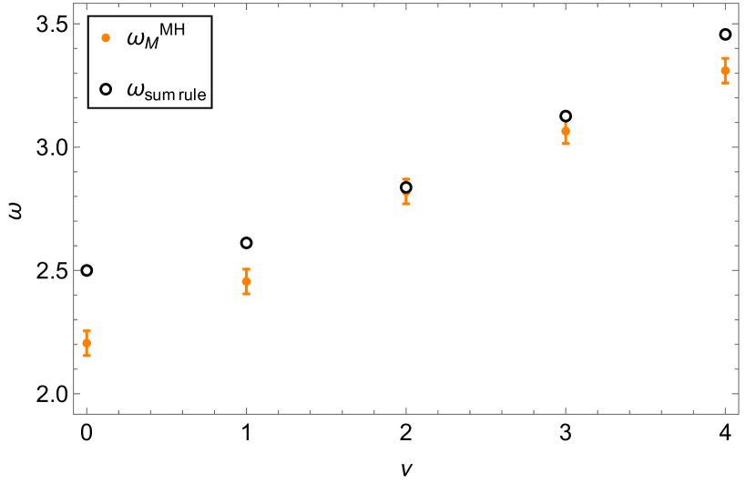
(a)

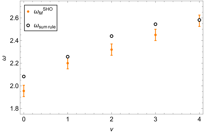
(b)

Figure 10: Comparison between the monopole frequency obtained with the numerical solutions of the GPE and the results of the sum rules predictions as given by Eq. (39). (a) MH with $\lambda=0.05$ and (b) SHO with $\rho_{0}=2.5$, both with the same interaction strength $G_{2D}=50$. The frequency increases with larger vorticities, indicating that vortices reduce the compressibility of the gas.

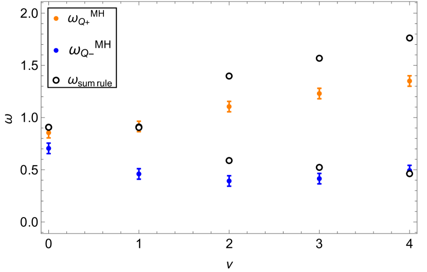
(a)

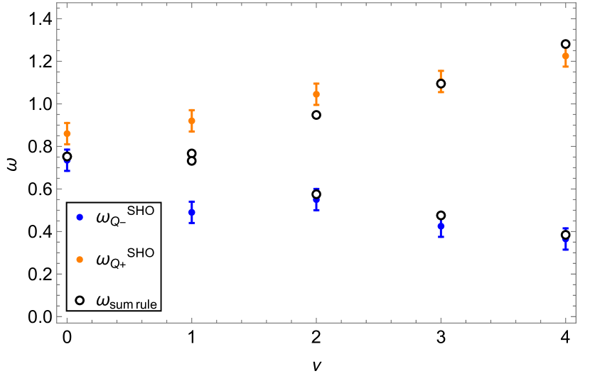
(b)

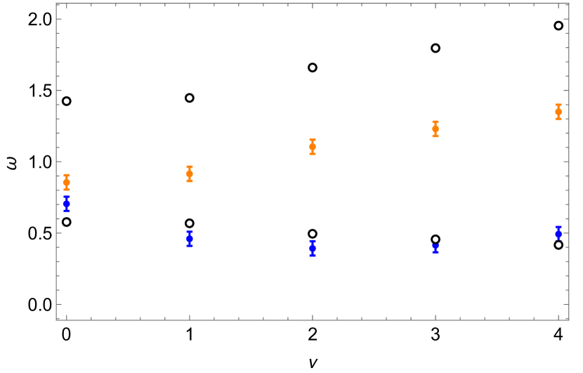
(c)

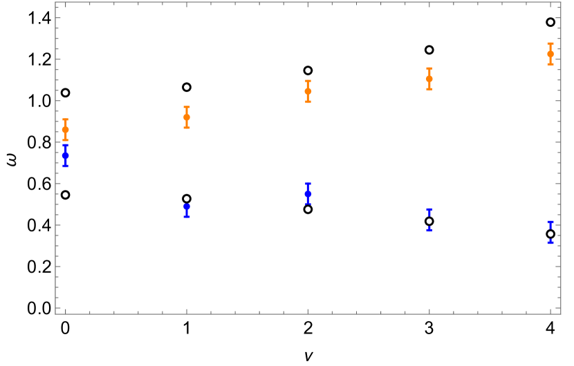
(d)

Figure 11: Comparison between the quadrupole frequency obtained with the numerical solution of the GPE, the results of the (a-b) two-modes quadrupole sum rule, Eq. (50), and the (c-d) four-modes quadrupole sum rule, Eq. (60). Panels (a) and (c) contain the results regarding the MH potential with $\lambda=0.05$, and (b) and (d) stand for the SHO potential with $\rho_{0}=2.5$. In both cases, we employed the same interaction strength $G_{2D}=50$. We can see that the splitting between the modes increases with increasing $\nu$, being proportional to the angular momentum. The four-modes approach better reproduces the numerical results.

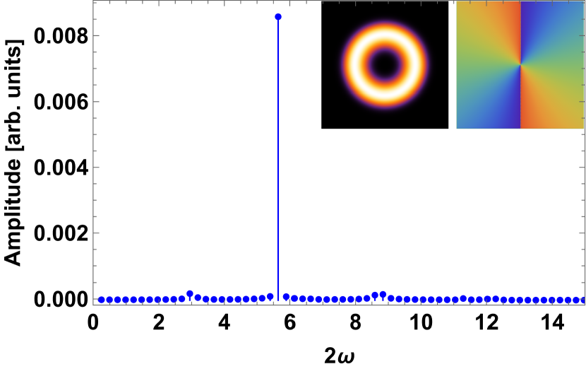
(a)

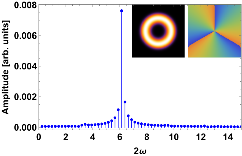
(b)

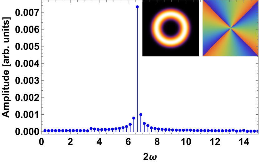
(c)

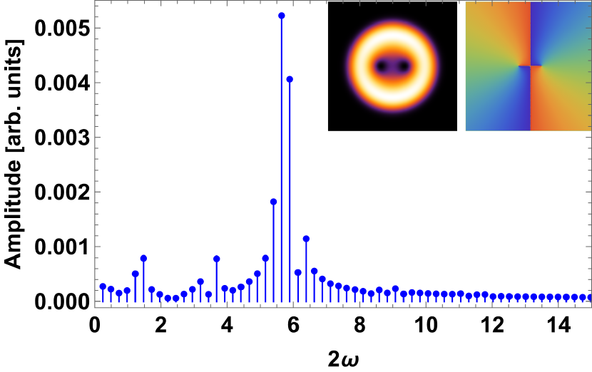
(d)

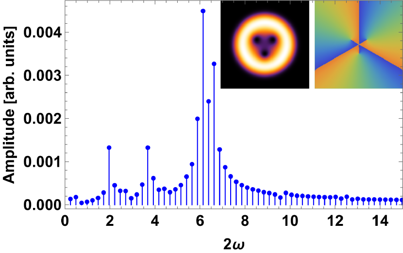
(e)

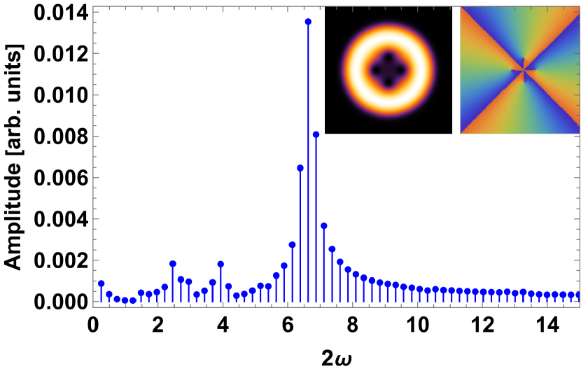
(f)

Figure 12: Monopole mode of the Mexican hat trap with $\lambda=0.05$. The interaction parameter is $G_{2D}=50$ for the (a-c) macrovortices and $G_{2D}=100$ for the (d-f) vortex lattices. The rotation frequencies are $\Omega=0.3$, $0.4$, and $0.5$ for panels (a) and (d), (b) and (e), (c) and (f), respectively. In the insets, we reproduce the density and phase profiles of the ground state.

A straightforward way of exciting collective modes is considering slightly different Hamiltonians in the imaginary and real time simulations. This means that the ground state obtained in the imaginary time simulation is not an eigenstate of the Hamiltonian used for the real time evolution. The subsequent dynamics are used to probe the collective modes. To observe the monopole mode, we increased the value of $G_{2D}$ by 20%. We introduced a small anisotropy in the trapping potential for the quadrupole mode, increasing the frequency in the $x$ direction by 5%. For each $\Omega$, $G_{2D}$, collective mode and trapping potential, we computed the wave function in $1024$ different instants, forming a time series. We extracted the frequency of the monopole mode $\omega_{\mathrm{M}}$ by performing a Fourier analysis of $\langle x^{2}\rangle$. Analogously, we obtained the quadrupole mode frequency $\omega_{\mathrm{Q}}$ by considering $\langle x^{2}-y^{2}\rangle/\langle x^{2}+y^{2}\rangle$.

In the following, we considered the MH with anharmonicity $\lambda=0.05$ and the SHO trap with the shift $\rho_{0}=2.5$. The resolution of the FFT technique gives the error bars in the numerical results. The predictions using sum rules correspond to the expressions of Eqs. (38) and (40) for the monopole, and Eqs. (50) and Eq.(60) for the quadrupole modes. These are functions of the partial energies of the system, which we calculated with the numerical ground state solution obtained with the imaginary time propagation of the GPE.

In Fig. 10, we show the monopole frequency of the macrovortex configuration as a function of the vorticity $\nu$, for the MH and SHO traps, with a fixed interaction strength $G_{2D}=50$. The sum rule prediction reasonably agrees with the numerical results for the MH and the SHO potential.

Regarding the quadrupole results, Fig. 11, we see the increase in the modes separation with the macrovortex vorticity $\nu$. The four-modes sum rule prediction, Eq. (60), is better suited to reproduce the numerical data when compared to the two-modes approach. However, for the MH trap, we observe the sum rule overestimation of the numerical results of the high-frequency branch. In the MH case, the higher modes coupling due to the anharmonic term is not negligible, indicating that we should include more modes in the sum rules derivation. It is worth remembering that the four-modes approach also accounted for the additional modes that appear due to the existence of two walls in the ring configuration, with very close frequencies, both showing the separation into its components $m=\pm 2$ as we increase the vorticity of the condensed cloud. However, as these modes have very close energy values, it is difficult to distinguish them, mostly for large $\Omega$, so we only include two energy branches, each representing the mixture of the $+2$ and $-2$ components of each wall mode.

It is important to note that Eq. (60) depends on the compressibility moment $m_{-1}$, for which the formula has not yet been presented. Unlike the other modes, this particular moment is not described in terms of partial energies. Its calculation is based on linear response theory, with the proper perturbation for each condensate mode, as detailed in Appendix B.

Finally, we compare the collective modes frequency of the macrovortex and the vortex lattice states for the same value of $\Omega$. While we used $G_{2D}=50$ for all the macrovortex configurations, to have stable vortex lattices, we had to increase the value of interaction to $G_{2D}=100$. Figure 12 contains the macrovortex and vortex lattice monopole frequency for three values of the rotation frequency $\Omega=0.3,0.4$, and $0.5$ in the MH trap. We observe that the well-defined peak of the macrovortex case evolves to a Lorentzian-shaped one in the corresponding vortex lattice configuration. The same situation is illustrated in Fig. 13, where we explored the frequency spectrum of the quadrupole mode in the SHO trap. The damping of the oscillations in the lattice case, i.e., the broadening of the collective mode peak, can be attributed to the appearance of additional modes due to the oscillation of the vortices. During the collective dynamics, the separation of the vortices and, consequently, their interaction will change over time. In this process, part of their energy can be transferred to the sound wave modes, keeping the total energy of the system constant.

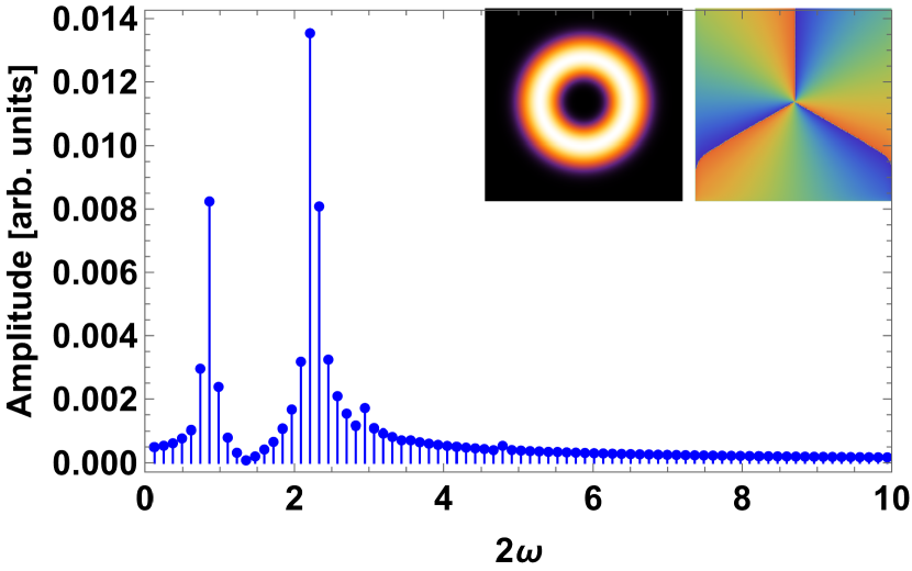
(a)

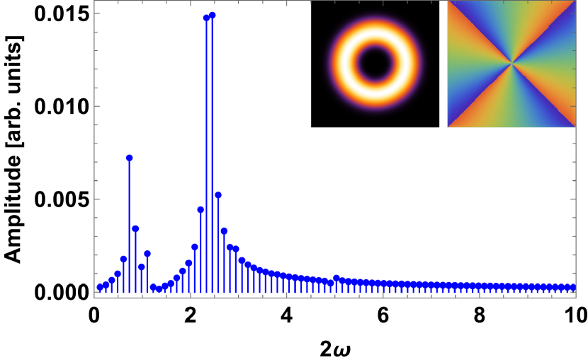
(b)

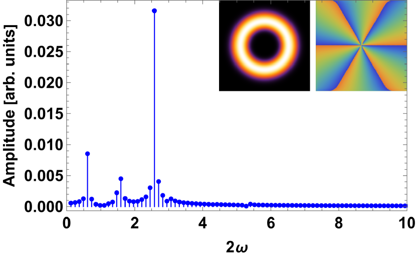
(c)

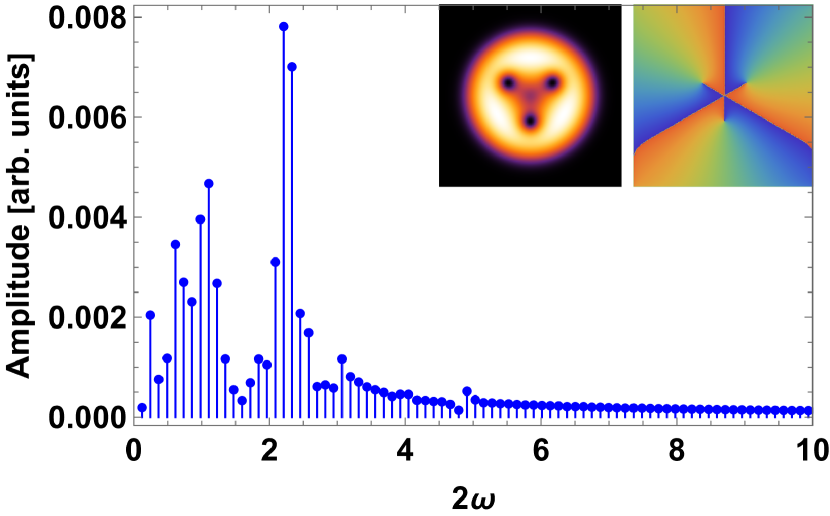
(d)

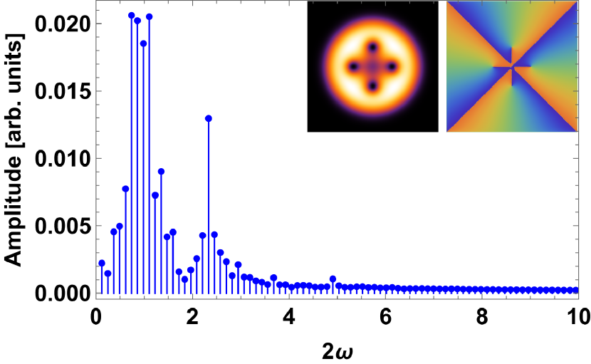
(e)

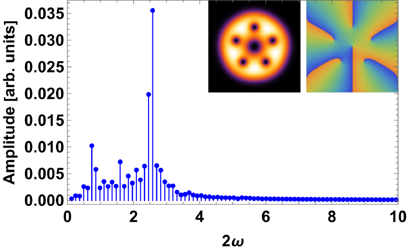
(f)

Figure 13: Quadrupole mode of the shifted harmonic oscillator with $\rho_{0}=2.5$. The interaction parameter is $G_{2D}=50$ for the (a-c) macrovortices and $G_{2D}=100$ for the (d-f) vortex lattices. The rotation frequencies are $\Omega=0.3$, $0.4$, and $0.5$ for panels (a) and (d), (b) and (e), (c) and (f), respectively. In the insets, we reproduce the density and phase profiles of the ground state.

V Conclusions

We studied the vortex configurations that appear in different ring confinements that can be implemented in bubble trap experiments. We used analytical and numerical calculations to determine the phase diagram of the system and its collective mode dynamics. We showed how the configuration of the vortices significantly affects the condensate ground state solution in the rotating frame and the frequency of the collective modes. The magnitude of the frequency of the monopole mode increases with the cloud vorticity, reflecting the lower compressibility of condensates with vortices. Also, we observed the damping of the collective modes associated with the vortex lattice formation, which can be an auxiliary method to probe the macrovortex to singly-charged vortex lattice transition in the experiments. We emphasise that the experimental conditions make the configuration of vortices hard to resolve in free-expansion and in-situ images due to the fast radial expansion of the rotating cloud Guo (2021).

In future works, we want to improve our variational phase diagram, including higher values for the external rotation and the atomic interaction to further map the experimental conditions. For that, we intend to use the Bogoliubov-de Gennes equations to track the dynamic instabilities of the system and then recalculate the phase diagram with less computational cost. We will also extend our analytical calculations to explore higher interaction regimes using the Thomas-Fermi (TF) ansatz for the ground-state solution. It will be interesting to compare the frequency evolution of the collective modes from the macrovortex to the TF-lattice regime. The latter has the vortex core and the lattice parameter (space between vortices) much smaller than the ring dimensions. While useful in many analyses, numerical methods have the disadvantage of not always elucidating the underlying physics, so an analytical expression for the frequencies of the modes is very desirable.

Appendix A Virial Theorem

In the following discussions, we restrict ourselves to a situation where $N$ particles are confined in a Mexican hat or a shifted harmonic potential and experience contact interactions described by a delta function. The Hamiltonian is given by Eq. (II.2), and we assume that the state of the system is stationary. We define the expectation value of a quantity $x$ as the usual inner product with the wave function, i.e., $\langle x\rangle\equiv\int d^{2}r\;\psi^{*}x\psi$. Then, the expectation value of $\sum_{i}\mathbf{q}_{i}\cdot\mathbf{p}_{i}$, with ${\bf{q}}_{i}$ corresponding to the generalized coordinates of the $i$-th particle, is constant in time,

$$\frac{d}{dt}\left\langle\sum_{i}\mathbf{q}_{i}\cdot\mathbf{p}_{i}\right\rangle=0.$$ (63)

On the other hand, Heisenberg’s equation of motion gives

$$\frac{d}{dt}\sum_{i}\mathbf{q}_{i}\cdot\mathbf{p}_{i}=\frac{i}{\hbar}\left[\hat{H},\sum_{i}\mathbf{q}_{i}\cdot\mathbf{p}_{i}\right].$$ (64)

We derived the Virial relation for two different trap potentials: the Mexican hat, Eq. (11), and the SHO, Eq. (20). For the MH trap,

$$E_{kin}+E_{int}+E_{ho}-\lambda\langle\rho^{4}\rangle=0,$$ (65)

which can be rewritten as

$$2E_{kin}-2E_{trap}^{MH}+2E_{int}-\lambda\langle\rho^{4}\rangle=0,$$ (66)

with

$$E_{trap}^{MH}=-\frac{1}{2}\langle\rho^{2}\rangle+\frac{\lambda}{2}\langle\rho^{4}\rangle.$$ (67)

On the other hand, for the SHO,

$$2E_{kin}+2E_{int}-2E_{ho}+\rho_{0}\langle\rho\rangle=0,$$ (68)

which can be rewritten as

$$2E_{kin}-2E_{trap}^{\rm SHO}+2E_{int}-\rho_{0}\langle\rho\rangle+\rho_{0}^{2}=0,$$ (69)

with

$$E_{trap}^{\rm SHO}=\frac{1}{2}\langle(\rho-\rho_{0})^{2}\rangle.$$ (70)

Appendix B Compressibility Sum Rules

The more accurate results for the sum rule frequencies involve the determination of the compressibility moment $m_{-1}$. Differently from $m_{1}$ and $m_{3}$, it is more convenient to relate the moment $m_{-1}$ to the static response function Pitaevskii and Stringari (2016). A rule for calculating $m_{-1}$ is through the explicit determination of the polarization.

B.1 Monopole

To calculate the ratio $m_{1}/m_{-1}$, which involves the inverse energy weighted moment, we considered

$$2m_{-1}=-\chi_{M}(0),$$ (71)

where the susceptibility $\chi_{M}(0)$ characterizes the static limit of the dynamic response function. For the moment $m_{1}$, we have the expression

$$m_{1}=\frac{2N\hbar^{2}\langle{\tilde{\rho}}^{2}\rangle}{\tilde{M}},$$ (72)

where $\tilde{M}$ corresponds to the mass of the particle and the mean value of the momentum squared is taken with respect to the ground state of the system.

To determine $\chi_{M}(0)$, first we considered the Hamiltonian of Eq. (II.2) with the perturbation

$$H_{pert}=\frac{1}{2}\tilde{M}\tilde{\omega}_{0}^{2}\gamma\sum_{i}\tilde{\rho}_{i}^{2}.$$ (73)

After, we applied the procedure to produce dimensionless quantities,

$$\tilde{\rho} = \tilde{\ell}_{\gamma}r_{1},$$

$$\tilde{\mu} = \mu_{1}\hbar\tilde{\omega}_{\gamma},$$

$$\tilde{\psi} = \sqrt{\frac{N}{\sqrt{2\pi}{Z}\tilde{\ell}_{\gamma}^{2}}}\psi_{1},$$

with $\tilde{\omega}_{\gamma}=(1+\gamma)^{1/2}\tilde{\omega}_{0}$ and $\tilde{\ell}_{\gamma}=\sqrt{\hbar/\tilde{M}\tilde{\omega}_{\gamma}}$.

We solved the corresponding time-independent GPE, obtained substituting $\psi_{1}(t)=\psi_{1}(0)e^{-\mu_{1}t}$ in Eq.(62). The term $\mathbf{\Omega}\cdot\mathbf{L}$ was replaced by $\mathbf{\Omega}\cdot\mathbf{r}\times\mathbf{v}$, where we considered the solid-body rotation $\mathbf{v}=\mathbf{\Omega}\times\mathbf{r}$. Using the TF approximation for the MH trap potential yields

$$n_{vl}^{MH}(r_{1})=|\psi_{1}|^{2}=\frac{\mu_{1}+\frac{1}{2}\left[\Omega_{1}^{2}r_{1}^{2}+r_{1}^{2}-\lambda_{1}(\tilde{\ell}_{\gamma})r_{1}^{4}\right]}{G_{2D}},$$ (74)

where

$$\lambda_{1}(\gamma)=\frac{\lambda\tilde{\ell}_{\gamma}^{2}}{(1+\gamma)},$$ (75)

and $\Omega_{1}=\tilde{\Omega}/\tilde{\omega}_{\gamma}$. For $\chi_{M}(0)$, we have the identity

$$\chi_{M}(0)=\frac{2N}{M}\frac{\partial\langle\tilde{\rho}^{2}\rangle}{\partial\tilde{\omega}_{\gamma}^{2}}\bigg{|}_{\gamma\rightarrow 0}=\frac{2N}{M}\frac{\partial\gamma}{\partial\tilde{\omega}_{\gamma}^{2}}\frac{\partial\langle\tilde{\rho}^{2}\rangle}{\partial\gamma}\bigg{|}_{\gamma\rightarrow 0}.$$ (76)

Then,

$$\frac{\partial\langle\tilde{\rho}^{2}\rangle}{\partial\gamma}=\frac{\partial[\tilde{\ell}_{\gamma}^{2}\langle r_{1}^{2}\rangle]}{\partial\gamma}=2\tilde{\ell}_{\gamma}\frac{\partial\tilde{\ell}_{\gamma}}{\partial\gamma}\langle r_{1}^{2}\rangle+\tilde{\ell}_{\gamma}^{2}\frac{\partial\langle r_{1}^{2}\rangle}{\partial\gamma}.$$ (77)

Angular momentum conservation gives

$$\frac{\partial}{\partial\gamma}[\Omega_{1}\langle r_{1}^{2}\rangle]=0.$$ (78)

Remembering that

$$\langle r_{1}^{2}\rangle=\frac{(1+\Omega_{1}^{2})}{2\lambda_{1}},$$ (79)

we get

$$\frac{m_{1}}{m_{-1}}=-2\hbar^{2}\tilde{\omega}_{0}^{2}\frac{\langle r_{1}^{2}\rangle\tilde{\ell}_{\gamma}^{2}}{2\tilde{\ell}_{\gamma}\frac{\partial\tilde{\ell}_{\gamma}}{\partial\gamma}\langle r_{1}^{2}\rangle+\frac{\tilde{\ell}_{\gamma}^{2}\frac{\partial\lambda_{1}}{\partial\gamma}\frac{\partial\langle r_{1}^{2}\rangle}{\partial\lambda_{1}}}{1+\frac{\Omega_{1}}{\langle r_{1}^{2}\rangle}\frac{\partial\langle r_{1}^{2}\rangle}{\partial\Omega_{1}}}}.$$ (80)

Then, taking the limit $\gamma\rightarrow 0$, yields

$$\sqrt{\frac{m_{1}}{m_{-1}}}=\hbar\tilde{\omega}_{0}\sqrt{6\Omega^{2}+2},$$ (81)

with $\Omega=\tilde{\Omega}/\tilde{\omega}_{0}$

Analogously for the SHO trap, with a TF density profile given by

$$n^{\rm SHO}_{vl}(r_{1})=\frac{\mu_{1}+\frac{1}{2}\left[\Omega_{1}^{2}r_{1}^{2}-r_{1}^{2}-\frac{1}{1+\gamma}({r}_{0}^{2}-2r_{1}{r}_{0})\right]}{G_{2D}},$$ (82)

where ${r}_{0}=\tilde{\rho}_{0}/\tilde{\ell}_{\gamma}$. We find

$$\sqrt{\frac{m_{1}}{m_{-1}}}=\hbar\tilde{\omega}_{0}\sqrt{\frac{12{\eta\prime}^{2}(1-{\Omega}^{2})^{3}+80r_{0}^{2}(1+3{\Omega}^{2})}{20r_{0}^{2}(5-{\Omega}^{2})-{\eta\prime}^{2}(1-{\Omega}^{2})^{3}}}.$$ (83)

where

$$\eta\prime=\left(\frac{6}{\pi}\frac{G_{2D}}{r_{0}}\right)^{1/3}.$$ (84)

B.2 Quadrupole

Using the same dimensionless quantities of the main text, we calculated the static quadrupole response through the perturbation with strength $\varepsilon$,

$$\delta V_{ext}=\frac{1}{2}\varepsilon(x^{2}-y^{2}),$$ (85)

which introduces an asymmetry in the confining potential. More specifically, we determined the compressibility mode by calculating the limit

$$m_{-1}^{+}={4N}\lim_{\varepsilon\rightarrow 0}\langle x^{2}+y^{2}\rangle\left(\frac{\partial\delta_{\varepsilon}}{\partial\varepsilon}\right),$$ (86)

where

$$\delta_{\varepsilon}=\frac{\langle y^{2}-x^{2}\rangle}{\langle x^{2}+y^{2}\rangle}.$$ (87)

First, we considered the perturbed density profile for the MH potential,

$$n_{vl}^{MH}\left(\rho\right) =\frac{\mu+\frac{{\Omega}^{2}}{2}\left(x^{2}+y^{2}\right)+\frac{1}{2}\left[\left(1+\varepsilon\right)x^{2}+\left(1-\varepsilon\right)y^{2}\right]}{G_{2D}}$$

$$-\frac{\frac{\lambda}{2}\left(x^{2}+y^{2}\right)^{2}}{G_{2D}}.$$ (88)

By using Eq. (86), it is straightforward to show that

$$m_{-1}^{+}=\frac{\pi N}{3G_{2D}}(R_{2}^{6}-R_{1}^{6}),$$ (89)

where the boundaries of the TF profile are $R_{1}$ and $R_{2}$, with $R_{2}>R_{1}$. Using the simplified notation $R_{\pm}^{2}=R_{2}^{2}\pm R_{1}^{2}$, we get

$$\frac{m_{1}^{+}}{m_{-1}^{+}}=4\lambda\frac{R_{+}^{2}R_{-}^{4}}{3R_{+}^{4}+R_{-}^{4}},$$ (90)

where we used that

$$m_{1}^{+}=8N\langle\rho^{2}\rangle.$$ (91)

Then, we applied the TF profile to determine the MH solution,

$$\sqrt{\frac{m_{1}^{+}}{m_{-1}^{+}}}=2\sqrt{\frac{(1+{\Omega}^{2})\eta^{2}}{3(1+{\Omega}^{2})^{2}+\eta^{2}}},$$ (92)

with

$$\eta=\left(\frac{12G_{2D}\lambda^{2}}{\pi}\right)^{1/3}.$$ (93)

On the other hand, for the macrovortex profile with charge $\nu$, we have

$$\sqrt{\frac{m_{1}^{+}}{m_{-1}^{+}}}=2{R_{-}^{2}}\sqrt{\frac{12\nu^{2}+R_{+}^{4}-R_{-}^{4}}{3R_{+}^{8}-2R_{-}^{4}R_{+}^{4}-R_{-}^{8}}}.$$ (94)

For the SHO case, considering the simplified notation of the ring mean radius $R=({R_{1}+R_{2}})/{2}$ and width $d=R_{2}-R_{1}$, we get

$$\sqrt{\frac{m_{1}^{+}}{m_{-1}^{+}}}=\sqrt{\frac{8(1-{\Omega}^{2})(3d^{4}+20R^{2}d^{2})}{5(3d^{4}+40d^{2}R^{2}+48R^{4})}}.$$ (95)

Whereas, if we consider the macrovortex profile,

$$\sqrt{\frac{m_{1}^{+}}{m_{-1}^{+}}}=\sqrt{\frac{8d^{2}\left[(d^{2}-4R^{2})^{2}(3d^{2}+20R^{2})-48(d^{2}-20R^{2})\nu^{2}\right]}{5(d^{2}-4R^{2})^{2}(3d^{4}+40d^{2}R^{2}+48R^{4})}}.$$ (96)

Appendix C Details of the moments calculations

The moments are given by

$$m_{1}^{+}=\langle 0|[F_{-},[H,F_{+}]]|0\rangle,$$

$$m_{2}^{-}=\langle 0|[[F_{-},H],[H,F_{+}]]|0\rangle,$$

$$m_{3}^{+}=\langle 0|[[F_{-},H],[H,[H,F_{+}]]]|0\rangle,$$

$$m_{4}^{-}=\langle 0|[[[F_{-},H],H],[H,[H,F_{+}]]]|0\rangle.$$ (97)

For the Mexican hat trap, we obtain

$$\frac{m_{2}^{-}}{m_{1}^{+}}=\left[\frac{1}{{\Omega}}\frac{E_{rot}}{E_{ho}}-4{\Omega}\right],$$

$$\frac{m_{3}^{+}}{m_{1}^{+}}=2\left[\frac{E_{kin}}{E_{ho}}-1+6{\Omega}^{2}-3\frac{E_{rot}}{E_{ho}}+3\lambda\frac{\langle\rho^{4}\rangle}{\langle\rho^{2}\rangle}\right],$$

$$\frac{m_{4}^{-}}{m_{2}^{-}}=4\bigg{\{}\frac{\frac{E_{kin}}{E_{ho}}-1+2{\Omega^{2}}-\frac{3}{2}\frac{E_{rot}}{E_{ho}}}{1-\frac{1}{4{\Omega}^{2}}\frac{E_{rot}}{E_{ho}}}$$

$$\qquad\qquad+\frac{\frac{1}{4{\Omega}^{2}}\frac{E_{rot}}{E_{ho}}-3\lambda\left(\frac{1}{2{\Omega}}\frac{\left\langle\rho^{2}{L}_{z}\right\rangle}{\left\langle{\rho}^{2}\right\rangle}-\frac{\left\langle\rho^{4}\right\rangle}{\left\langle\rho^{2}\right\rangle}\right)}{1-\frac{1}{4{\Omega}^{2}}\frac{E_{rot}}{E_{ho}}}\bigg{\}}.$$ (98)

For the SHO trap, we have

$$\frac{m_{2}^{-}}{m_{1}^{+}}=\left[\frac{1}{{\Omega}}\frac{E_{rot}}{E_{ho}}-4{\Omega}\right],$$ (99)

$$\frac{m_{3}^{+}}{m_{1}^{+}}=2\left[\frac{E_{kin}}{E_{ho}}+1+6{\Omega}^{2}-3\frac{E_{rot}}{E_{ho}}-\frac{3}{4}\rho_{0}\frac{\langle\rho\rangle}{\langle\rho^{2}\rangle}\right],$$

$$\frac{m_{4}^{-}}{m_{2}^{-}}=4\bigg{\{}\frac{\frac{E_{kin}}{E_{ho}}+1+2{\Omega^{2}}-\frac{3}{2}\frac{E_{rot}}{E_{ho}}}{1-\frac{1}{4{\Omega}^{2}}\frac{E_{rot}}{E_{ho}}}$$

$$\qquad\qquad-\frac{\frac{1}{4{\Omega}^{2}}\frac{E_{rot}}{E_{ho}}-\frac{3}{4}\rho_{0}\left(\frac{1}{2{\Omega}}\frac{\left\langle{L}_{z}/\rho\right\rangle}{\left\langle{\rho}^{2}\right\rangle}-\frac{\left\langle\rho\right\rangle}{\left\langle\rho^{2}\right\rangle}\right)}{1-\frac{1}{4{\Omega}^{2}}\frac{E_{rot}}{E_{ho}}}\bigg{\}}.$$ (100)

In the equations above, we have the rotational energy,

$$E_{rot}=\Omega\langle L_{z}\rangle,$$ (101)

with the angular momentum given by

$$L_{z}=\left(x\,p_{y}-p_{x}\,y\right).$$ (102)

We also used the identity

$$\frac{\langle L_{z}\rangle}{2\Omega\langle\rho^{2}\rangle}=\frac{1}{4\Omega^{2}}\frac{E_{rot}}{E_{ho}}.$$ (103)

References

• Landau and Lifshitz (1976) L. D. Landau and E. M. Lifshitz, Mechanics, 3rd ed. (Pergamon Press, Moscow, 1976) p. 170.
• Pitaevskii and Stringari (2016) L. Pitaevskii and S. Stringari, Bose-Einstein Condensation and Superfluidity (Oxford University Press, 2016).
• Pethick and Smith (2008) C. J. Pethick and H. Smith, Bose-Einstein Condensation in Dilute Gases (Cambridge University Press, 2008).
• Anderson et al. (1995) M. H. Anderson, J. R. Ensher, M. R. Matthews, C. E. Wieman,  and E. A. Cornell, Observation of Bose-Einstein condensation in a dilute atomic vaporScience 269, 198 (1995).
• Davis et al. (1995) K. B. Davis, M. O. Mewes, M. R. Andrews, N. J. van Druten, D. S. Durfee, D. M. Kurn,  and W. Ketterle, Bose-Einstein Condensation in a Gas of Sodium AtomsPhys. Rev. Lett. 75, 3969 (1995).
• Bradley et al. (1995) C. C. Bradley, C. A. Sackett, J. J. Tollett,  and R. G. Hulet, Evidence of Bose-Einstein Condensation in an Atomic Gas with Attractive InteractionsPhys. Rev. Lett. 75, 1687 (1995).
• Abo-Shaeer et al. (2001) J. R. Abo-Shaeer, C. Raman, J. M. Vogels,  and W. Ketterle, Observation of Vortex Lattices in Bose-Einstein CondensatesScience 292, 476 (2001).
• Butts and Rokhsar (1999) D. A. Butts and D. S. Rokhsar, Predicted signatures of rotating Bose–Einstein condensatesNature 397, 327 (1999).
• Fetter (2008) A. L. Fetter, Rotating trapped Bose-Einstein condensatesLaser Phys. 18, 1 (2008).
• Tong (2016) D. Tong, Lectures on the Quantum Hall Effect (2016)arXiv:1606.06687 .
• Danaila (2005) I. Danaila, Three-dimensional vortex structure of a fast rotating Bose-Einstein condensate with harmonic-plus-quartic confinementPhys. Rev. A 72, 013605 (2005).
• Cozzini (2006) M. Cozzini, Diffused vorticity approach to the oscillations of a rotating Bose-Einstein condensate confined in a harmonic plus quartic trapPramana 66, 31 (2006).
• Fetter (2001) A. L. Fetter, Rotating vortex lattice in a Bose-Einstein condensate trapped in combined quadratic and quartic radial potentialsPhys. Rev. A 64, 063608 (2001).
• Fu and Zaremba (2006) H. Fu and E. Zaremba, Transition to the giant vortex state in a harmonic-plus-quartic trapPhys. Rev. A 73, 013614 (2006).
• Aftalion and Danaila (2004) A. Aftalion and I. Danaila, Giant vortices in combined harmonic and quartic trapsPhys. Rev. A 69, 033608 (2004).
• Zobay and Garraway (2001) O. Zobay and B. M. Garraway, Two-dimensional atom trapping in field-induced adiabatic potentialsPhys. Rev. Lett. 86, 1195 (2001).
• Zobay and Garraway (2004) O. Zobay and B. M. Garraway, Atom trapping and two-dimensional Bose-Einstein condensates in field-induced adiabatic potentialsPhys. Rev. A. 69, 15 (2004).
• Colombe et al. (2004) Y. Colombe, E. Knyazchyan, O. Morizot, B. Mercier, V. Lorent,  and H. Perrin, Ultracold atoms confined in rf-induced two-dimensional trapping potentialsEPL 67, 593 (2004).
• Garraway and Perrin (2016) B. M. Garraway and H. Perrin, Recent developments in trapping and manipulation of atoms with adiabatic potentialsJ. Phys. B 49, 172001 (2016).
• Perrin and Garraway (2017) H. Perrin and B. M. Garraway, Trapping Atoms With Radio Frequency Adiabatic Potentials, in Adv. At. Mol. Opt. Phys., Vol. 66 (2017) pp. 181–262.
• Padavić et al. (2018) K. Padavić, K. Sun, C. Lannert,  and S. Vishveshwara, Physics of hollow Bose-Einstein condensatesEPL 120, 20004 (2018).
• Sun et al. (2018) K. Sun, K. Padavić, F. Yang, S. Vishveshwara,  and C. Lannert, Static and dynamic properties of shell-shaped condensatesPhys. Rev. A. 98, 013609 (2018).
• Lundh (2002) E. Lundh, Multiply quantized vortices in trapped Bose-Einstein condensatesPhys. Rev. A 65, 043604 (2002)0103272 .
• Jackson et al. (2004) A. D. Jackson, G. M. Kavoulakis,  and E. Lundh, Phase diagram of a rotating Bose-Einstein condensate with anharmonic confinementPhys. Rev. A. 69, 053619 (2004).
• Herve (2018) M. d. G. Herve, Superfluid dynamics of annular Bose gases, Ph.D. thesis, Université Paris 13, Paris (2018).
• de Goër de Herve et al. (2021) M. de Goër de Herve, Y. Guo, C. De Rossi, A. Kumar, T. Badr, R. Dubessy, L. Longchambon,  and H. Perrin, A versatile ring trap for quantum gasesJ. Phys. B 54, 125302 (2021).
• Carollo et al. (2022) R. A. Carollo, D. C. Aveline, B. Rhyno, S. Vishveshwara, C. Lannert, J. D. Murphree, E. R. Elliott, J. R. Williams, R. J. Thompson,  and N. Lundblad, Observation of ultracold atomic bubbles in orbital microgravityNature 606, 281 (2022).
• Guo et al. (2020) Y. Guo, R. Dubessy, M. d. G. de Herve, A. Kumar, T. Badr, A. Perrin, L. Longchambon,  and H. Perrin, Supersonic Rotation of a Superfluid: A Long-Lived Dynamical RingPhys. Rev. Lett. 124, 025301 (2020).
• Jin et al. (1996) D. S. Jin, J. R. Ensher, M. R. Matthews, C. E. Wieman,  and E. A. Cornell, Collective Excitations of a Bose-Einstein Condensate in a Dilute GasPhys. Rev. Lett. 77, 420 (1996).
• Mewes et al. (1996) M.-O. Mewes, M. R. Andrews, N. J. van Druten, D. M. Kurn, D. S. Durfee, C. G. Townsend,  and W. Ketterle, Collective Excitations of a Bose-Einstein Condensate in a Magnetic TrapPhys. Rev. Lett. 77, 988 (1996).
• Marzlin et al. (1997) K.-P. Marzlin, W. Zhang,  and E. M. Wright, Vortex Coupler for Atomic Bose-Einstein CondensatesPhys. Rev. Lett. 79, 4728 (1997)9708198 .
• Dum et al. (1998) R. Dum, J. I. Cirac, M. Lewenstein,  and P. Zoller, Creation of Dark Solitons and Vortices in Bose-Einstein CondensatesPhys. Rev. Lett. 80, 2972 (1998).
• Jackson and Kavoulakis (2004) A. D. Jackson and G. M. Kavoulakis, Vortices and hysteresis in a rotating Bose-Einstein condensate with anharmonic confinementPhys. Rev. A. 70, 023601 (2004).
• Lipparini and Stringari (1989) E. Lipparini and S. Stringari, Sum rules and giant resonances in nucleiPhys. Rep. 175, 103 (1989).
• Zambelli and Stringari (1998) F. Zambelli and S. Stringari, Quantized Vortices and Collective Oscillations of a Trapped Bose-Einstein CondensatePhys. Rev. Lett. 81, 1754 (1998).
• Kishor Kumar et al. (2019) R. Kishor Kumar, V. Lončar, P. Muruganandam, S. K. Adhikari,  and A. Balaž, C and Fortran OpenMP programs for rotating Bose-Einstein condensatesComput. Phys. Commun. 240, 74 (2019).
• Guo (2021) Y. Guo, Annular quantum gases in a bubble-shaped trap: from equilibrium to strong rotations.Ph.D. thesis (2021).