Standoff Tracking Using DNN-Based MPC with Implementation on FPGA

Abstract

This work studies the standoff tracking problem to drive an unmanned aerial vehicle (UAV) to slide on a desired circle over a moving target at a constant height. We propose a novel Lyapunov guidance vector (LGV) field with tunable convergence rates for the UAV’s trajectory planning and a deep neural network (DNN)-based model predictive control (MPC) scheme to track the reference trajectory. Then, we show how to collect samples for training the DNN offline and design an integral module (IM) to refine the tracking performance of our DNN-based MPC. Moreover, the hardware-in-the-loop (HIL) simulation with an FPGA@$200$$\mathrm{M}\mathrm{H}\mathrm{z}$ demonstrates that our method is a valid alternative to embedded implementations of MPC for addressing complex systems and applications which is impossible for directly solving the MPC optimization problems.

I Introduction

Using unmanned aerial vehicles (UAVs) for convoy protection and aerial surveillance has attracted broad attention. To achieve it, it is essential for the UAV to standoff track a moving target, which not only permits a persistent tracking but also expands its surveillance area. In the literature, it is also called the target circumnavigation or encirclement [1, 2, 3, 4].

The first of this strategy lies in designing a good guidance law. In [5], a Lyapunov guidance vector (LGV) is initially proposed and then extended in [6, 7, 8]. The issue on the non-adjustable convergence rate of these works is resolved in [9] with a gradient-based method. In this work, we directly propose a new LGV with easily tunable convergence rates, which contains the GVs in [5, 6, 7, 8] as a special case.

The second is to regulate the UAV to track the LGV in the complex environment subject to dynamics constraint and state-control vector constraints. If there is no constraint, it is conceivable to utilize the backstepping controller by regarding the guidance law as the reference signal. For example, Ref. [10] adopts a structure of five backstepping steps that resembles the multi-loop proportional-integral-derivative (PID) controller in [11, 12, 13]. While they cannot explicitly handle the state and control constraints, the model predictive control (MPC) becomes a natural alternative [14]. Since the MPC law is usually obtained by solving online optimization problems, it is only applicable to “simple” systems with moderate sizes [15, 16, 17, 18, 19]. If the size of the MPC optimization problem is small for linear time-invariant (LTI) system, the so-called explicit MPC [18] appears to be perfect as its control law has a piece-wise affine (PWA) form, meaning that it can be obtained via a simple search over a finite number of polyhedra. Unfortunately, this number grows exponentially with respect to the MPC size, including the numbers of prediction horizons, decision variables and their constraints. For instance, such a number is up to $1638$ for a single-input LTI system with $4$ box-constrained states and $10$ prediction horizon [19].

How to implement the MPC on a resource-limited embedded platform in a fast and faithful way is a long-standing problem. With the development of the deep learning and the advanced RISC machine (ARM) or field-programmable gate array (FPGA), such a problem has attracted resurgent interest. Roughly speaking, the related works can be categorized into two types of approaches, depending on whether the MPC law is computed iteratively or approximated via a deep neural network (DNN). The works on developing tailored iterative solvers for an embedded platform include [20, 21, 22, 23]. Specifically, Ref. [22] exploits the structure of the MPC optimization problem and develops PRESAS for online solving the sequential quadratic programs (QP). A particle swarm optimization (PSO) method is designed in [23] to search the MPC solution in parallel.

The other alternative that is closely related to this work is on the use of an offline trained DNN to implement the MPC law. For example, a DNN is trained to approximate the PWA function of the explicit MPC law in [19], and a primal-dual learning framework is proposed in [24] to regulate a linear parameter-varying system. In fact, the DNN-based MPC has demonstrated promising results on resonant power converters [25], PMSMs [26], and UAVs [27] whose DNN-based MPC is however only evaluated on a high-performance NVIDIA TX2 CPU@$2$$\mathrm{G}\mathrm{H}\mathrm{z}$ with Pytorch. Moreover, the DNN is adopted to warm start a sequence of primal active-set algorithms in [28]. Note that it is also unknown how many iterations are required to obtain a certifiable solution of the MPC optimization problem. In [29], a correction factor is further introduced, hoping to achieve offset-free set-point tracking. Clearly, there is a tradeoff between the approximation error of the MPC law and the size of the DNN, which is key to the performance of the closed-loop system, and how to quantify their relationship remains an open problem.

In contrast to the aforementioned works, we first adopt a DNN-based MPC for the UAV to track our LGV and then design a simple integral module (IM) to refine the tracking performance. Since we aim at the UAV’s resource-limited onboard implementation, the DNN size cannot be too large which inevitably induces approximation errors. Thus, we do not expect that the DNN-based MPC is able to exactly track our LGV and thus propose the IM to further reduce the steady-state tracking error, allowing to use a relatively small size of the DNN. The idea is presented in the preliminary version of this article in [30]. Table I indeed clarifies the computing efficiency of implementing our DNN-based MPC on an FPGA. To speedup the use of an FGPA for a control designer, we introduce a verification and implementation framework that enables to directly generate and verify verilog codes from algorithms developed in MATLAB. Moreover, the hardware-in-the-loop (HIL) simulation with an FPGA@$200$$\mathrm{M}\mathrm{H}\mathrm{z}$ demonstrates that our method is a valid alternative to embedded implementations of MPC for managing complex systems and applications. Overall, our contributions are summarized as follows.

TABLE I: A comparison of the existing works.

Ref.	Method	Systems	$\mathrm{dim}(\bm{x})$	$\mathrm{dim}(\bm{u})$	$N_{p}$	$N_{c}$	Platform	Latency	Latency (200$\mathrm{M}\mathrm{H}\mathrm{z}$)1
[16]	Active-set	Linear	2	2	3	1	F28335 DSP ($150$$\mathrm{M}\mathrm{H}\mathrm{z}$)	$<0.3$$\mathrm{m}\mathrm{s}$	$<0.23$$\mathrm{m}\mathrm{s}$
[22]	PRESAS	Nonlinear	11	4	20	20	ARM Cortex-A7 ($900$$\mathrm{M}\mathrm{H}\mathrm{z}$)	$6.44$$\mathrm{m}\mathrm{s}$	$28.98$$\mathrm{m}\mathrm{s}$
[23]	PSO	Nonlinear	3	3	5	1	ARM Cortex-A9 ($800$$\mathrm{M}\mathrm{H}\mathrm{z}$)	$60.62$$\mathrm{m}\mathrm{s}$	$242.48$$\mathrm{m}\mathrm{s}$
							Altera FPGA ($50$$\mathrm{M}\mathrm{H}\mathrm{z}$)	$1.09$$\mathrm{m}\mathrm{s}$	$0.27$$\mathrm{m}\mathrm{s}$
[19]	DNN	Linear	4	1	10	10	ARM Cortex-M0 ($48$$\mathrm{M}\mathrm{H}\mathrm{z}$)	$3.8$$\mathrm{m}\mathrm{s}$	$0.912$$\mathrm{m}\mathrm{s}$
[24]	DNN	Linear	4	3	3	3	TC27x ECU DSP ($200$$\mathrm{M}\mathrm{H}\mathrm{z}$)	$1.8$$\mathrm{m}\mathrm{s}$	$1.8$$\mathrm{m}\mathrm{s}$
[25]	DNN	Nonlinear	2	2	10	10	FPGA2	$2.1\upmu$$\mathrm{s}$	–
[27]	DNN	Linear	8	3	30	30	NVIDIA TX2 CPU3  ($2$$\mathrm{G}\mathrm{H}\mathrm{z}$)	$1.66$$\mathrm{m}\mathrm{s}$	$16.6$$\mathrm{m}\mathrm{s}$
This work	DNN	Nonlinear	12	4	20	10	ARM Cortex-A53 ($200$$\mathrm{M}\mathrm{H}\mathrm{z}$)	$1.030$$\mathrm{m}\mathrm{s}$	$1.030$$\mathrm{m}\mathrm{s}$
							Zynq FPGA ($200$$\mathrm{M}\mathrm{H}\mathrm{z}$)	$0.126$$\mathrm{m}\mathrm{s}$	$0.126$$\mathrm{m}\mathrm{s}$

• Eq. (9) in [20] is adopted to covert the reported latency in the reference work to that on the same type processor @200$\mathrm{M}\mathrm{H}\mathrm{z}$.

• The specifics of FPGA are not provided in [25].

• The NVIDIA TX2 CPU contains a dual-core NVIDIA Denver 2 processor @$2$$\mathrm{G}\mathrm{H}\mathrm{z}$ and a quad-core ARM Cortex-A57 processor @$2$$\mathrm{G}\mathrm{H}\mathrm{z}$.

• A novel LGV law with tunable convergence rates is proposed for standoff tracking a moving target, which covers the GV in [5, 6, 7, 8] as a special case.

• We propose a DNN-based MPC with a simple IM to track the LGV.

• An easily accessible framework is introduced for fast generating and verifying verilog codes from algorithms developed in MATLAB.

The rest of the paper is organized as follows. In Section II, we describe the standoff tracking problem. We propose a new LGV for planning the standoff tracking trajectory in Section III and design MPCs to track the reference trajectory in Section IV. In Section V, we collect training samples and propose a DNN-based MPC with an IM track our LGV. The HIL simulation with an FPGA@$200$$\mathrm{M}\mathrm{H}\mathrm{z}$ is performed in Section VI, and some conclusion remarks are drawn in Section VII.

Notation: Throughout this paper, scalars, vectors, and matrices are respectively denoted by lowercase letters, lowercase bold letters, and uppercase letters, e.g. $a$, $\bm{a}$, and $A$. The vectors $\bm{0}_{n},\bm{1}_{n}$ and the matrix $I_{n}$ denote the zero and one vectors and an identity matrix with specified dimensions. The superscript $(\cdot)^{\text{T}}$ represents the matrix transpose. The symbol $\|\cdot\|$ denotes the Euclidean norm. The function $\text{col}(\cdot)$ and $\text{blkdiag}(\cdot)$ return a column vector by stacking each vector on top of the other and a block diagonal matrix, respectively. For a vector $\bm{x}$, then $\bm{x}\in[0,\bar{x}]$ means that every element of $\bm{x}$ belongs to this interval. Moreover, $\bm{x}(t)$ and $\bm{x}(k)$ represent the continuous- and discrete-time state vectors with the relation that $t=t_{0}+k\tau$, where $t_{0}$ is the initial time instant and $\tau$ is the sampling period. The vector ${\bm{x}}(i|k)$ represents the predicted state at time step $k+i$ based on $\bm{x}(k)$.

II Problem Formulation

The standoff tracking of this work requires a quadrotor UAV to slide on a desired circle over a moving target at a constant height, and is also called the target circumnavigation or target encirclement in [1, 3, 2, 4].

II-A The kinematic model of the moving target

The moving target of interest travels in the single-integrator form

$$\dot{\bm{p}}_{o}(t)=\bm{v}_{o}(t),$$ (1)

where $\bm{p}_{o}(t)=[x_{o}(t),y_{o}(t),z_{o}(t)]^{\text{T}}$ and $\bm{v}_{o}(t)\in\mathbb{R}^{3}$ respectively denote its position and velocity.

II-B The dynamical model of the quadrotor UAV

To standoff track the target in (1), we adopt a quadrotor UAV in [11] whose Newton-Euler dynamical model is expressed by

$$\begin{split}\ddot{\bm{\xi}}(t)=&\bm{g}+{m}^{-1}\left(R(\bm{\eta}(t))\bm{t}_{b}(t)-\text{diag}(d_{x},d_{y},d_{z})\dot{\bm{\xi}}(t)\right),\\ \ddot{\bm{\eta}}(t)=&J^{-1}(\bm{\eta}(t))\left(\bm{\tau}_{b}(t)-C(\bm{\eta}(t),\dot{\bm{\eta}}(t))\dot{\bm{\eta}}(t)\right),\end{split}$$ (2)

where ${\bm{\xi}}(t)=[x_{q}(t),y_{q}(t),z_{q}(t)]^{\text{T}}$, $\bm{\eta}(t)=[\phi(t),\theta(t),\psi(t)]^{\text{T}}$ denote the 3D position and the vector of Euler angles in the inertial frame, respectively. $R(\bm{\eta}(t))$, $J(\bm{\eta}(t))$, $C(\bm{\eta}(t),\dot{\bm{\eta}}(t))$, $\bm{t}_{b}(t)$, and $\bm{\tau}_{b}(t)$ denote the rotation matrix from the body frame to the inertial frame, the Jacobian matrix, the Coriolis matrix, the total thrust and torque in the body frame, respectively. Moreover, $\bm{t}_{b}(t)$ and $\bm{\tau}_{b}(t)$ are determined by the control input to the rotor in the following form

$$\begin{split}\bm{t}_{b}(t)&=\begin{bmatrix}0,&0,&l_{c}\sum_{i=1}^{4}u_{i}(t)\end{bmatrix}^{\text{T}}\in\mathbb{R}^{3},\\ \bm{\tau}_{b}(t)&=\begin{bmatrix}l\cdot l_{c}\left(-u_{2}(t)+u_{4}(t)\right)\\ l\cdot l_{c}\left(-u_{1}(t)+u_{3}(t)\right)\\ d_{c}\left(-u_{1}(t)+u_{2}(t)-u_{3}(t)+u_{4}(t)\right)\end{bmatrix}\in\mathbb{R}^{3},\end{split}$$ (3)

where $\bm{u}(t)=[u_{1}(t),u_{2}(t),u_{3}(t),u_{4}(t)]^{\text{T}}\in[0,\bar{u}]$ and other unspecified quantities are constant parameters. More details of (2) can be found in [11, Chapter 2]. In simulations, we directly obtain the codes from [31] for the UAV’s dynamics with a sampling period $\tau=0.1$.

II-C The objective of standoff tracking

Let the relative 3D position between the target and UAV be

$$[x(t),y(t),z(t)]^{\text{T}}=[x_{q}(t)-x_{o}(t),y_{q}(t)-y_{o}(t),z_{q}(t)-z_{o}(t)]^{\text{T}}$$ (4)

and define their relative velocity and distance in the horizon plane as

$$\bm{v}(t)=[\dot{x}(t),\dot{y}(t)]^{\text{T}},~{}~{}r(t)=\left(x^{2}(t)+y^{2}(t)\right)^{1/2}.$$ (5)

Then, the standoff tracking requires the UAV in (2) to loiter over the target in (1) such that

$$\lim_{t\rightarrow\infty}r(t)=r_{d},~{}\lim_{t\rightarrow\infty}z(t)=z_{d},~{}~{}\lim_{t\rightarrow\infty}\|\bm{v}(t)\|=v_{d},$$ (6)

where the triple $[r_{d},z_{d},r_{d}]^{\text{T}}$ denotes the desired standoff tracking pattern.

To achieve (6), the maximum of the UAV’s speed $\|\dot{\bm{\xi}}(t)\|$ is assumed to be sufficiently greater than that of the target [6], and the UAV is able to localize the target with onboard sensors [8].

III Lyapunov Guidance Vector for Standoff Tracking

In general, the guidance commands for the standoff tracking of the UAV are separately designed in the horizontal plane and its vertical direction. Since the guidance in the vertical direction is trivial, this section focuses on the guidance design in the horizontal plane via a new LGV.

III-A The gradient-based LGV

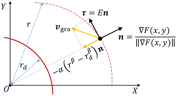
Figure 1: Illustration of the gradient-based LGV in (10).

We build a Cartesian frame with the target position as its origin and define a scalar field as follows

$$F(x,y)=x^{2}+y^{2}.$$ (7)

Then, the objective of $\lim_{t\rightarrow\infty}r(t)=r_{d}$ requires the UAV to slide on the following isoline [32]

$$\mathcal{L}(r_{d})=\left\{[x,y]^{\text{T}}\in\mathbb{R}^{2}|F(x,y)=r_{d}^{2}\right\},$$

which is represented by the red solid arc in Fig. 1. To this goal, a term of $-\alpha\left(r^{\beta}(t)-r_{d}^{\beta}\right){\bm{n}}(t)$ is naturally needed for the GV to pull the UAV towards $\mathcal{L}(r_{d})$ at the negative gradient direction with a force depending on the error of $r^{\beta}(t)-r_{d}^{\beta}$, where $\alpha$ is a positive parameter, $\beta\in\mathbb{N}_{+}$ is a constant exponent, $r(t)$ is the range (c.f. (5)) from the UAV to the target, and $\bm{n}(t)$ denotes the unit gradient vector, i.e.,

$${\bm{n}}(t)=\frac{\nabla F(x(t),y(t))}{\|\nabla F(x(t),y(t))\|}=\begin{bmatrix}x(t)/r(t)\\ y(t)/r(t)\end{bmatrix}$$ (8)

where $\nabla F(x,y)=\begin{bmatrix}2x,2y\end{bmatrix}^{{\mathrm{T}}}$ is the gradient of (7). If the UAV reaches $\mathcal{L}(r_{d})$, i.e., $r(t)=r_{d}$, it is required to move along $\mathcal{L}(r_{d})$. Thus, an orthogonal vector $\bm{\tau}(t)$ to the unit gradient vector ${\bm{n}}(t)$ is further introduced, i.e.,

$${\bm{\tau}}(t)= \begin{bmatrix}\cos\gamma&-\sin\gamma\\ \sin\gamma&\cos\gamma\end{bmatrix}{\bm{n}}(t)=E{\bm{n}}(t),$$ (9)

where $\gamma=\pi/2$ or $-\pi/2$ determines the rotation angle and without loss of generality, we set $\gamma=\pi/2$ in this work.

Then, we design a GV as follows

$$\bm{v}_{\text{gra}}(t)={\bm{\tau}}(t)-\alpha\left(r^{\beta}(t)-r_{d}^{\beta}\right){\bm{n}}(t).$$ (10)

See Fig. 1 for an illustration.

For the objective of $\lim_{t\rightarrow\infty}\|\bm{v}(t)\|=v_{d}$, we scale (10) as

$$\bar{\bm{v}}_{\text{gra}}(t)=v_{d}\frac{\bm{v}_{\text{gra}}(t)}{\|\bm{v}_{\text{gra}}(t)\|}$$

$$=\frac{-v_{d}/r(t)}{\sqrt{1+\alpha^{2}\left(r^{\beta}(t)-r_{d}^{\beta}\right)^{2}}}\begin{bmatrix}\alpha x(t)\left(r^{\beta}(t)-r_{d}^{\beta}\right)-y(t)\\ \alpha y(t)\left(r^{\beta}(t)-r_{d}^{\beta}\right)+x(t)\end{bmatrix}.$$

Instead of using a constant $\alpha$ in [13], we further use its time-varying version to accelerate the GV convergence, i.e.,

$$\alpha(t)=\left({4r^{\beta}(t)r_{d}^{\beta}}\right)^{-1/2}.$$ (11)

Inserting (11) into $\bar{\bm{v}}_{\text{gra}}(t)$ yields our LGV, i.e.,

$$\begin{split}\bm{v}_{L}(t)=&~{}\frac{-v_{d}}{r(t)\left(r^{\beta}(t)+r_{d}^{\beta}\right)}\\ &\times\begin{bmatrix}x(t)\left(r^{\beta}(t)-r_{d}^{\beta}\right)+2y(t)\sqrt{r^{\beta}(t)r_{d}^{\beta}}\\ y(t)\left(r^{\beta}(t)-r_{d}^{\beta}\right)-2x(t)\sqrt{r^{\beta}(t)r_{d}^{\beta}}\end{bmatrix}.\end{split}$$ (12)

Lemma 1

Consider a stationary target located at $[x_{o},y_{o}]^{\text{T}}$ and the position $[x_{q}(t),y_{q}(t)]^{\text{T}}$ governed by the LGV in (12), i.e., $[\dot{x}_{q}(t),\dot{y}_{q}(t)]^{\text{T}}=\bm{v}_{L}(t)$. Then, it holds that

$$\lim_{t\rightarrow\infty}r^{\beta}(t)=r_{d}^{\beta}~{}\text{and}~{}\lim_{t\rightarrow\infty}v(t)=v_{d}$$

where $v(t)=\|\bm{v}(t)\|$, and $r(t),\bm{v}(t)$ are given in (5).

Proof:

First, $\lim_{t\rightarrow\infty}v(t)=v_{d}$ trivially holds as it follows from (12) that $\|\bm{v}_{L}(t)\|=v_{d}$. Then, we consider a Lyapunov function candidate as

$$L_{1}(r(t))=\frac{1}{2}\left(r^{\beta}(t)-r_{d}^{\beta}\right)^{2},$$ (13)

and take its derivative along with (12)

$$\dot{L}_{1}(r(t)) =\beta r^{\beta-1}(t)\left(r^{\beta}(t)-r_{d}^{\beta}\right){r^{-1}(t)}[x(t),y(t)]^{\text{T}}\bm{v}_{L}(t)$$

$$=-\frac{2\beta v_{d}r^{\beta-1}(t)}{r^{\beta}(t)+r_{d}^{\beta}}L_{1}(r(t))$$ (14)

$$\leq 0.$$

Clearly, $L_{1}(r_{d})=0$, and $L_{1}(r(t))>0$ for any $r(t)\neq r_{d}$. By [33, Theorem 4.2], it implies that $r^{\beta}(t)$ asymptotically converges to $r_{d}^{\beta}$, i.e., $\lim_{t\rightarrow\infty}r^{\beta}(t)=r_{d}^{\beta}$.  

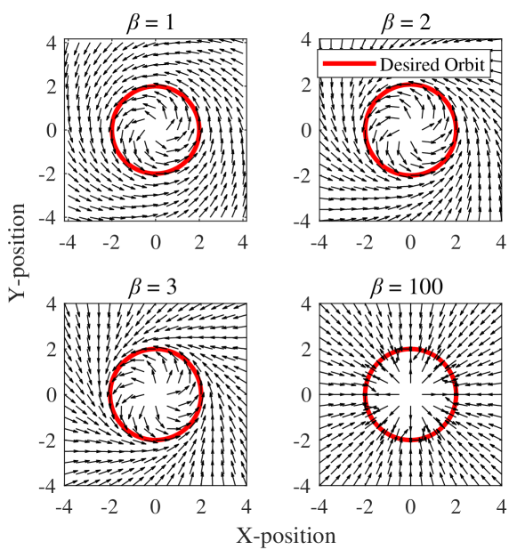
Figure 2: The LGV fields with different exponents $\beta\in\{1,2,3,100\}$.

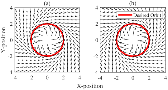
Figure 3: The LGV fields: (a) the counterclockwise direction; (b) the clockwise direction.

If $r(t)\geq r_{d}$, which usually holds for $t=t_{0}$ in the standoff tracking problem [34], it follows from (III-A) that

$$\dot{L}_{1}(r(t))\leq-\left({\beta v_{d}}/{r_{d}}\right)L_{1}(r(t)).$$ (15)

Jointly with (13), it implies that the larger $\beta$, the faster the decreasing rate of $r(t)$ to $r_{d}$. On the other hand, if $r(t)<r_{d}$, one can easily obtain that $\dot{L}_{1}(r(t))>-\left({\beta v_{d}}/{r_{d}}\right)L_{1}(r(t)).$ Jointly with Lemma 1 and (13), it implies that $r(t)$ will increase to $r_{d}$ with an exponential rate faster than ${\beta v_{d}}/{r_{d}}$. From this perspective, increasing $\beta$ can speed up the convergence of the LGV, which is also verified by Fig. 2. Since there are physical input limits for the UAV in (2), e.g., ${\bm{u}}(t)\in[0,\bar{u}]$, the UAV cannot follow an LGV with an arbitrarily large $\beta$. In fact, $|\dot{r}(t)|\leq v_{d}$ implies that the convergence rate of the LGV has an upper bound. The fastest one needs manual tuning to match this limit as there is no theoretical result to justify how to achieve it. Note that there is a trade-off between the convergence rate and the computational burden in (12). In our simulations, we fix $\beta=3$ for an illustration. Interestingly, the case of $\beta=2$ leads to the GV method in [6, 7, 8]. Thus, we not only further justify their design but also generalize it to obtain faster convergence rates. A discrete-time version of (12) with $\beta=2$ is also devised in our previous work [8], where the sampling frequency should be faster than an explicit lower bound to ensure its effectiveness.

The LGV field in (12) will guide the UAV to encircle the target in a counterclockwise direction. If the desired direction is clockwise, we simply let $\gamma=-\pi/2$ in (8) and the LGV is modified as

$$\begin{split}\bm{v}_{L}(t)=&~{}\frac{-v_{d}}{r(t)\left(r^{\beta}(t)+r_{d}^{\beta}\right)}\\ &\times\begin{bmatrix}x(t)\left(r^{\beta}(t)-r_{d}^{\beta}\right)-2y(t)\sqrt{r^{\beta}(t)r_{d}^{\beta}}\\ y(t)\left(r^{\beta}(t)-r_{d}^{\beta}\right)+2x(t)\sqrt{r^{\beta}(t)r_{d}^{\beta}}\end{bmatrix}.\end{split}$$ (16)

See Fig. 3 for an illustration. There is no loss of generality to select any direction, as one can achieve the same results for the other direction. Note that if the controller continuously switches its direction, it will potentially destabilize the closed-loop system.

III-B The Justification of our LGV from the geometry perspective

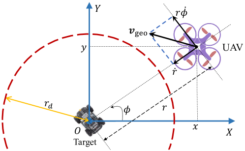
Figure 4: Coordinate frame centered at the target.

We further justify our LGV in (12) from the geometry perspective. As illustrated in Fig. 4, we establish a polar frame centered at the target and denote the coordinates of the UAV by the radius $r(t)$ and angle $\phi(t)$, respectively. Then, their relative position $x(t)=x_{q}(t)-x_{o}(t)$ and $y(t)=y_{q}(t)-y_{o}(t)$ on the horizon plane are expressed as

$$x(t)=r(t)\cos\phi(t)~{}\text{and}~{}y(t)=r(t)\sin\phi(t).$$

Taking the time derivative of $x(t)$ and $y(t)$ leads to that

$$\begin{bmatrix}\dot{x}(t)\\ \dot{y}(t)\end{bmatrix}=\begin{bmatrix}\cos\phi(t)&-\sin\phi(t)\\ \sin\phi(t)&\cos\phi(t)\end{bmatrix}\begin{bmatrix}\dot{r}(t)\\ r(t)\dot{\phi}(t)\end{bmatrix}\triangleq\bm{v}_{\text{geo}}(t).$$ (17)

Thus, we can first design the radial velocity $\dot{r}(t)$ and tangential velocity $r(t)\dot{\phi}(t)$ in the polar frame and then convert them into the Cartesian frame by the rotation matrix in (17).

Consider the following Lyapunov function candidate

$$L_{2}(r(t))=\frac{1}{2}\left(r^{\beta}(t)-r_{d}^{\beta}\right)^{2}.$$ (18)

Taking the derivative of $L_{2}(r(t))$ yields that

$$\dot{L}_{2}(r(t))=\beta\left(r^{\beta}(t)-r_{d}^{\beta}\right)r^{\beta-1}(t)\dot{r}(t).$$ (19)

To ensure the negativeness of $\dot{L}_{2}(r(t))$, we design the radial velocity $\dot{r}(t)$ as

$$\dot{r}(t)=-\alpha v_{d}\left(r^{\beta}(t)-r_{d}^{\beta}\right),~{}\alpha>0.$$ (20)

It immediately follows from (20) that

$$\dot{L}_{2}(r(t))=-\alpha\beta v_{d}r^{\beta-1}(t)\left(r^{\beta}(t)-r_{d}^{\beta}\right)^{2},~{}\lim_{t\rightarrow\infty}r^{\beta}(t)=r_{d}^{\beta}.$$

Moreover, let the tangential velocity $r(t)\dot{\phi}(t)$ satisfy that

$$\dot{r}^{2}(t)+\left(r(t)\dot{\phi}(t)\right)^{2}=v_{d}^{2}.$$ (21)

By (20), it requires that $\alpha\left(r^{\beta}(t)-r_{d}^{\beta}\right)\leq 1$ for any $r(t)>0$. To this end, we select $\alpha$ as

$$\alpha=\left(r^{\beta}(t)+r_{d}^{\beta}\right)^{-1}.$$ (22)

Inserting (22) into (20) and (21) yields the following radial and tangential velocities

$$\begin{split}\dot{r}(t)=-v_{d}\frac{r^{\beta}(t)-r_{d}^{\beta}}{r^{\beta}(t)+r_{d}^{\beta}},~{}r(t)\dot{\phi}(t)=\pm v_{d}\frac{2\sqrt{r^{\beta}(t)r_{d}^{\beta}}}{r^{\beta}(t)+r_{d}^{\beta}}\end{split}.$$ (23)

Note that the direction of $\dot{r}(t)$ always points to the desired circle, i.e., the red one in Fig. 1, and that of $r(t)\dot{\phi}(t)$ needs to be manually specified as either the counterclockwise “$+$” or clockwise “$-$” direction. This is consistent with the value selection of $\gamma$ in (9). Combining (17) with (23), one can easily obtain the LGV in (12) and (16).

III-C Trajectory planning by the LGV

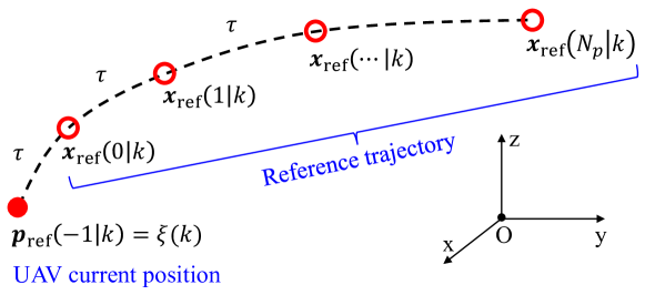
Figure 5: Illustration of trajectory planning by the LGV.

At the UAV position $\bm{\xi}(k)$, a reference trajectory is planned via the discretized LGV in (12) with a sampling period $\tau$, i.e.,

$$\bm{x}_{\text{ref}}(i|k)=\begin{bmatrix}\bm{p}_{\text{ref}}^{\text{T}}(i|k),\bm{0}_{3}^{\text{T}},\bm{v}_{\text{ref}}^{\text{T}}(i|k),\bm{0}_{3}^{\text{T}}\end{bmatrix}^{\text{T}},~{}i=0,1,\ldots,N_{p}$$

where $\bm{p}_{\text{ref}}(i|k)=[x_{\text{ref}}(i|k),y_{\text{ref}}(i|k),z_{\text{ref}}(i|k)]^{\text{T}}$ and $\bm{v}_{\text{ref}}(i|k)\in\mathbb{R}^{3}$ denote the predicted reference position and velocity at the $i$-th time-step ahead, respectively. Moreover, the reference Euler angles and rates are always set to zero for the stability consideration of the UAV.

Accordingly, define the predicted relative position and distance as

$$[x(i|k),y(i|k),z(i|k)]^{\text{T}} =\bm{p}_{\text{ref}}(i|k)-\bm{p}_{o}(i|k)$$

$$r(i|k) =\left(x^{2}(i|k)+y^{2}(i|k)\right)^{1/2}.$$

By replacing $x(t)$ and $y(t)$ in (12) with $x(i|k)$ and $y(i|k)$, the predicted LGV is naturally given below

$$\begin{split}&\bm{v}_{L}(i+1|k)=\frac{-v_{d}}{r(i|k)\left(r^{\beta}(i|k)+r_{d}^{\beta}\right)}\\ &~{}~{}~{}\times\begin{bmatrix}x(i|k)\left(r^{\beta}(i|k)-r_{d}^{\beta}\right)+2y(i|k)\sqrt{r^{\beta}(i|k)r_{d}^{\beta}}\\ y(i|k)\left(r^{\beta}(i|k)-r_{d}^{\beta}\right)-2x(i|k)\sqrt{r^{\beta}(i|k)r_{d}^{\beta}}\end{bmatrix}.\end{split}$$ (24)

Next, we show how to update the required quantities in (24). Firstly, it follows from (12) that the reference velocity $\bm{v}_{\text{ref}}(i+1|k)$ is updated as

$$\bm{v}_{\text{ref}}(i+1|k)=\begin{bmatrix}\bm{v}_{L}(i+1|k)\\ v_{z}\cdot\tanh\left(z_{d}-z(i|k)\right)\end{bmatrix}+\bm{v}_{o}(k),$$ (25)

where $v_{z}$ is a predefined vertical speed. Note that the standard hyperbolic tangent function $\tanh(\cdot)$ is adopted to ensure the boundedness of $\|\bm{v}_{\text{ref}}(i|k)\|$, i.e.,

$$\|\bm{v}_{\text{ref}}(i|k)\|\leq(v_{d}^{2}+v_{z}^{2})^{1/2}+\|\bm{v}_{o}(k)\|.$$

If the UAV is faster than the above upper bound, then $\bm{v}_{\text{ref}}(i|k)$ is feasible for the UAV.

Secondly, the reference position is initialized as $\bm{p}_{\text{ref}}(-1|k)=\bm{\xi}(k)$ (cf. Fig. 5) and updated via a single-integrator. That is

$$\bm{p}_{\text{ref}}(i+1|k)=\bm{p}_{\text{ref}}(i|k)+\tau\cdot\bm{v}_{\text{ref}}(i+1|k).$$ (26)

Note that we have shifted $\bm{v}_{\text{ref}}(\cdot|k)$ one step ahead for notational convenience. If $\tau$ is sufficiently small, it follows from [8, Theorem 1] that the reference trajectory $\{\bm{x}_{\text{ref}}(i|k)\}_{i=0}^{N_{p}}$ will guide the UAV to achieve (6).

Thirdly, we simply assume that the target velocity is invariant in the trajectory planning horizon and predict the target position as

$${\bm{p}}_{o}(i+1|k)={\bm{p}}_{o}(i|k)+\tau{\bm{v}_{o}(k)}~{}\text{with}~{}{\bm{p}}_{o}(-1|k)=\bm{p}_{o}(k).$$

Overall, our trajectory planning is fully described in Algorithm 1, where time indices of $x,y,z,r$ are omitted for brevity.

Algorithm 1 Trajectory planning by the LGV.

1. Input: the UAV position $\bm{\xi}(k)$, the target state $[\bm{p}_{o}^{\text{T}}(k),\bm{v}_{o}^{\text{T}}(k)]^{\text{T}}$, the desired tracking formation vector $[r_{d},z_{d},v_{d}]^{\text{T}}$.

2. Output: the reference trajectory $\{\bm{x}_{\text{ref}}(i|k)\}_{i=0}^{N_{p}}$.

   • initialization: Let $\bm{p}_{\text{ref}}(-1|k)=\bm{\xi}(k)$, and ${\bm{p}}_{o}(-1|k)=\bm{p}_{o}(k)$.

   • Update: For $i=-1,0,1,\ldots,N_{p}-1$

     • Compute the relative position and projected distance:

       $$[x,y,z]^{\text{T}} =\bm{p}_{\text{ref}}(i|k)-{\bm{p}}_{o}(i|k),$$

       $$r =\sqrt{x^{2}+y^{2}}.$$

     • Compute the predicted LGV by (12), i.e.,

       $$\bm{v}_{L}(i+1|k)=\frac{-v_{d}}{r(r^{\beta}+r_{d}^{\beta})}\begin{bmatrix}x(r^{\beta}-r_{d}^{n})+y(2\sqrt{r^{\beta}r_{d}^{\beta}})\\ y(r^{\beta}-r_{d}^{\beta})-x(2\sqrt{r^{\beta}r_{d}^{\beta}})\end{bmatrix}.$$

     • Compute the next desired states by (25):

       $$\bm{v}_{\text{ref}}(i+1|k) =\begin{bmatrix}\bm{v}_{L}(i+1|k)\\ v_{z}\cdot\tanh\left(z_{d}-z\right)\end{bmatrix}+{\bm{v}_{o}(k)},$$

       $$\bm{p}_{\text{ref}}(i+1|k) =\bm{p}_{\text{ref}}(i|k)+\tau\bm{v}_{\text{ref}}(i+1|k),$$

       $${\bm{p}}_{o}(i+1|k) ={\bm{p}}_{o}(i|k)+\tau{\bm{v}_{o}(k)}.$$

IV The Design of MPCs

In this section, we design both nonlinear and linearized MPCs to track the reference trajectory $\{\bm{x}_{\text{ref}}(i|k)\}_{i=0}^{N_{p}}$ in Algorithm 1.

IV-A The nonlinear MPC

Let $\bm{x}(t)=\text{col}\left(\bm{\xi}(t),\bm{\eta}(t),\dot{\bm{\xi}}(t),\dot{\bm{\eta}}(t)\right)$. We rewrite the model in (2) into the following abstract form

$$\dot{\bm{x}}(t)=f(\bm{x}(t),\bm{u}(t)),$$ (27)

and use the explicit Euler method to discretize it

$${\bm{x}}(k+1)={\bm{x}}(k)+\tau\cdot f(\bm{x}(k),\bm{u}(k)).$$ (28)

Then, our objective is on the control design to track the reference states $\{\bm{x}_{\text{ref}}(i|k)\}_{i=0}^{N_{p}}$. To this end, define the control input sequence as $\bm{u}(\cdot|k)=\left\{\bm{u}(0|k),\bm{u}(1|k),\ldots,\bm{u}(N_{p}-1|k)\right\}$ and the objective function as follows

$$J(\bm{u}(\cdot|k))= \frac{1}{2}\sum_{i=0}^{N_{p}}\left(\bm{x}(i|k)-\bm{x}_{\text{ref}}(i|k)\right)^{\text{T}}Q\left(\bm{x}(i|k)-\bm{x}_{\text{ref}}(i|k)\right)$$

$$+\frac{1}{2}\sum_{i=0}^{N_{p}-1}\left(\bm{u}(i|k)-\bm{u}_{\text{ref}}\right)^{\text{T}}R\left(\bm{u}(i|k)-\bm{u}_{\text{ref}}\right)$$

where $\bm{u}_{\text{ref}}=u_{\text{ref}}\cdot{\bm{1}}_{4}^{\text{T}}$ is a constant input vector for the UAV to ensure that $\bm{\eta}(t)=\dot{\bm{\xi}}(t)=\ddot{\bm{\xi}}(t)=0$ in (2), leading to $u_{\text{ref}}=mg/(4l_{c})$. Moreover, $Q$ and $R$ are positive semi-definite and positive definite weighting matrices, respectively.

The nonlinear MPC law is obtained by solving the constrained optimization problem per time-step $k$ viz

$$\bm{u}_{*}(\cdot|k)=\operatorname*{argmin}_{\bm{u}(\cdot|k)}J(\bm{u}(\cdot|k))$$ (29a)

$$~{}~{}~{}\mathrm{s.t.}~{}\bm{x}(0|k)=\bm{x}(k),$$ (29b)

$$~{}~{}~{}~{}~{}~{}~{}~{}\bm{x}(i+1|k)=\bm{x}(i|k)+\tau f(\bm{x}(i|k),\bm{u}(i|k)),$$ (29c)

$$~{}~{}~{}~{}~{}~{}~{}~{}\phi(i|k),\theta(i|k)\in[-c,c],$$ (29d)

$$~{}~{}~{}~{}~{}~{}~{}~{}\bm{u}(i|k)\in[0,\bar{u}],$$ (29e)

$$~{}~{}~{}~{}~{}~{}~{}~{}\bm{u}(j+1|k)=\bm{u}(j|k),~{}\forall j\geq N_{c}-1,$$ (29f)

where (29d) represents the constraint on pitch and roll angles of the UAV, and (29e) denotes the input constraint. In addition, $N_{p}$ and $N_{c}$ denote the tunable prediction and control horizons. To reduce the numerical complexity of (29), we omit the terminal cost and constraint set [35, 16] whose effect diminishes as the horizon length grows.

IV-B The linearized MPC

Since it is hard to directly solve the NLP in (29), one may consider to converting into a quadratic program (QP) by linearizing (28) at the current state $\bm{x}(k)$ as

$$\bm{x}(k+1)=A_{k}\bm{x}(k)+B_{k}\bm{u}(k),$$

where

$$A_{k}=I_{12}+\tau\frac{\partial f(\bm{x}(k),\bm{u}(k))}{\partial\bm{x}}~{}\text{and}~{}B_{k}=\tau\frac{\partial f(\bm{x}(k),\bm{u}(k))}{\partial\bm{u}}.$$

Then, the nonlinear model in (29c) is approximated by the following linearized prediction model

$$\bm{x}(i+1|k)=A_{k}\bm{x}(i|k)+B_{k}\bm{u}(i|k).$$ (30)

Note that other solutions can also be applied to limit the effect of prediction errors, e.g., linearization around a trajectory or robust approaches [14].

By letting $\Delta\bm{x}(i|k)=\bm{x}(i|k)-\bm{x}_{\text{ref}}(i|k)$ and $\Delta\bm{u}(i|k)=\bm{u}(i|k)-\bm{u}_{\text{ref}}$, we transform (30) into a LIT system, i.e.,

$$\Delta\bm{x}(i+1|k)=A_{k}\Delta\bm{x}(i|k)+B_{k}\Delta\bm{u}(i|k)+\bm{r}(i+1|k)$$ (31)

where $\bm{r}(i+1|k)$ is a nonzero offset and is given by

$$\bm{r}(i+1|k)=A_{k}\bm{x}_{\text{ref}}(i|k)+B_{k}\bm{u}_{\text{ref}}-\bm{x}_{\text{ref}}(i+1|k).$$

We define

$$\Delta X =\text{col}\left(\Delta\bm{x}(1|k),\ldots,\Delta\bm{x}(N_{p}|k)\right),$$

$$\Delta U =\text{col}\left(\Delta\bm{u}(0|k),\ldots,\Delta\bm{u}(N_{c}-1|k)\right),$$

and write (31) into a collected vector form

$$\Delta X=\widetilde{A}_{k}\Delta\bm{x}(0|k)+\widetilde{B}_{k}\Delta U+\widetilde{D}_{k},$$ (32)

where $\widetilde{A}_{k}$ and $\widetilde{B}_{k}$ are given in (33), and $\widetilde{D}_{k}$ is obtained by

$$\widetilde{D}_{k}=\begin{bmatrix}\bm{r}(1|k)\\ A_{k}\bm{r}(1|k)+\bm{r}(2|k)\\ \vdots\\ A_{k}^{N_{p}-1}\bm{r}(1|k)+A_{k}^{N_{p}-2}\bm{r}(2|k)+\ldots+\bm{r}(N_{p}|k)\end{bmatrix}.$$

$$\widetilde{A}_{k}=\begin{bmatrix}A_{k}\\ A_{k}^{2}\\ \vdots\\ A_{k}^{N_{p}}\end{bmatrix},~{}~{}\widetilde{B}_{k}=\begin{bmatrix}B_{k}&0&\cdots&0\\ A_{k}B_{k}&B_{k}&\ldots&0\\ \vdots&\vdots&\ddots&\vdots\\ A_{k}^{N_{c}-1}B_{k}&A_{k}^{N_{c}-2}B_{k}&\cdots&B_{k}\\ A_{k}^{N_{c}}B_{k}&A_{k}^{N_{c}-1}B_{k}&\cdots&A_{k}B_{k}+B_{k}\\ \vdots&\vdots&\ddots&\vdots\\ A_{k}^{N_{p}-1}B_{k}&A_{k}^{N_{p}-2}B_{k}&\cdots&A_{k}^{N_{p}-N_{c}}B_{k}+\cdots+A_{k}B_{k}+B_{k}\end{bmatrix}.$$ (33)

Letting $C\bm{x}(i|k)\leq\bm{c}$ represent the state constraint in (29d) and $\text{blkdiag}(\cdot)$ be a block diagonal matrix, the state constraint is rewritten as

$$\widetilde{C}\widetilde{B}_{k}\Delta U\leq\widetilde{\bm{c}}-\widetilde{C}\widetilde{A}_{k}\Delta\bm{x}(0|k)-\widetilde{C}\widetilde{D}_{k},$$ (34)

where $\widetilde{C}=\text{blkdiag}\left(C,\ldots,C\right)$ and

$$\widetilde{\bm{c}}=\text{col}\left(\bm{c},\ldots,\bm{c}\right)-\widetilde{C}\text{col}\left(\bm{x}_{\text{ref}}(1|k),\ldots,\bm{x}_{\text{ref}}(N_{p}|k)\right).$$

By (32) and (34), the NLP in (29) is converted into the following QP problem

$$\Delta U_{*}=\operatorname*{argmin}_{\Delta U}\frac{1}{2}\Delta U^{\text{T}}H\Delta U+\bm{h}^{\text{T}}\Delta U$$ (35a)

$$~{}~{}~{}\mathrm{s.t.}~{}~{}W\Delta U\leq\bm{w}.$$ (35b)

Here the new weighting matrix $H$ and vector $\bm{h}$ are given by

$$H=\widetilde{B}_{k}^{\text{T}}\widetilde{Q}\widetilde{B}_{k}+\widetilde{R},~{}\bm{h}=\widetilde{B}_{k}^{\text{T}}\widetilde{Q}^{\text{T}}\left(\widetilde{A}_{k}\Delta\bm{x}(0|k)+\widetilde{D}_{k}\right),$$

where $\widetilde{Q}=\text{blkdiag}(Q,\ldots,Q),~{}\widetilde{R}=\text{blkdiag}(R,\ldots,R)$ and the matrix $W$ and vector $\bm{w}$ in constraint (35b) are given by

$$W=\begin{bmatrix}\widetilde{C}\widetilde{B}_{k}\\ I_{4}\\ -I_{4}\end{bmatrix},~{}~{}\bm{w}=\begin{bmatrix}\widetilde{\bm{c}}-\widetilde{C}\widetilde{A}_{k}\Delta\bm{x}(0|k)-\widetilde{C}\widetilde{D}_{k}\\ (\bar{u}-u_{\text{ref}})\bm{1}_{4}\\ u_{\text{ref}}\bm{1}_{4}\end{bmatrix}.$$

IV-C Numerical comparison between the nonlinear and linearized MPCs in MATLAB

TABLE II: Comparison between the nonlinear and linearized MPCs on Intel Core i5-6500 CPU@$3.2$$\mathrm{G}\mathrm{H}\mathrm{z}$.

Horizon length		Solution time (s)		Range error (m)		Speed error (m/s)		Height error (m)
$N_{p}$	$N_{c}$	NMPC	LMPC	NMPC	LMPC	NMPC	LMPC	NMPC	LMPC
$10$	$5$	$0.0903$	$0.0067$	$0.1144$	$0.0420$	$0.0076$	$0.0101$	$0.0013$	$0.0091$
$10$	$10$	$0.1712$	${0.0070}$	$0.1115$	$0.0449$	${\bf 0.0075}$	$0.0099$	$0.0012$	$0.0093$
${\bf 20}$	${\bf 10}$	$0.3778$	$0.0089$	$0.0165$	$0.0209$	$0.0114$	$0.0250$	$1.71\times 10^{-4}$	$0.0090$
${20}$	${20}$	${0.6481}$	${0.0100}$	$0.0180$	$0.0264$	$0.0111$	$0.0242$	$\bm{1.28\times 10^{-4}}$	$0.0090$
$40$	$20$	$2.1852$	$0.0116$	${\bf 0.0124}$	$0.0534$	$0.0177$	$0.0258$	$5.21\times 10^{-4}$	$0.0090$
$40$	$40$	$2.6402$	$0.0145$	$0.0127$	$0.0573$	$0.0174$	$0.0235$	$5.27\times 10^{-4}$	$0.0090$

For comparing the nonlinear MPC in (29) with its linearized counterpart in (35), let $Q=\text{diag}(\bm{1}_{9},\bm{0}_{3})$, $R=0.1\cdot I_{4}$, $c=\pi/4$, $\bar{u}=12$ and the standoff tracking pattern is specified by $r_{d}=2.0$$\mathrm{m}$, $z_{d}=5.0$$\mathrm{m}$, $v_{d}=1.0$$\mathrm{m}\mathrm{/}\mathrm{s}$. In this simulation, they are solved by directly invoking nlmpcmove and quadprog in MATLAB 2020a on the personal computer with an Intel Core i5-6500 CPU@$3.2$$\mathrm{G}\mathrm{H}\mathrm{z}$. The steady-state tracking results are reported in Table II. Though the nonlinear MPC indeed outperforms the linearized one, their steady-state tracking performances are not significantly different for the horizon length up to $40$ ($=4$ seconds). We only report the transition results in Figs. 12-16 for their DNN-based versions for the purpose of saving space.

TABLE III: Solution time comparison between the nonlinear, linearized and DNN-based MPCs with $N_{p}=20$, $N_{c}=10$, $\tau=0.1$$\mathrm{s}$.

Platform	Intel Core i5@$3.2$$\mathrm{G}\mathrm{H}\mathrm{z}$			ARM@$200$$\mathrm{M}\mathrm{H}\mathrm{z}$			FPGA@$200$$\mathrm{M}\mathrm{H}\mathrm{z}$
Methods	NMPC	LMPC	DNN-based MPC	NMPC	LMPC	DNN–based MPC	DNN–based MPC
Solution time (s)	$0.3778$	$0.0089$	${\bf 2.81\times 10^{-5}}$	$120.9$	$2.8$	${\bf 1.03\times 10^{-4}}$	${\bf 1.26\times 10^{-4}}$

V The DNN-based MPC with an IM

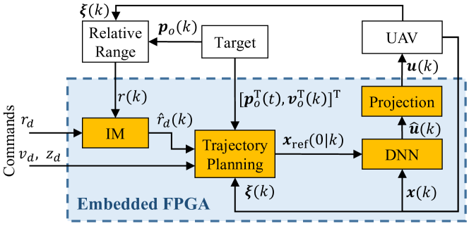
Figure 6: The standoff tracking system closed by the embedded trajectory planning and DNN-based MPC with an IM on an FPGA.

Although the solution efficiency of the QP in (35) is significantly improved over the NLP in (29), it is still challenging for an embedded processor, e.g., ARM or FPGA. For example, it follows from [36] and Eq. (9) in [20] that it requires at least $2.5\times 93.58=233.95$$\mathrm{m}\mathrm{s}$ for an ARM@$200$$\mathrm{M}\mathrm{H}\mathrm{z}$ to solve an QP in (35) with $\mathrm{dim}(\bm{x})=12$, $\mathrm{dim}(\bm{u})=4$, and $N_{p}=N_{c}=20$, which is impossible to complete within a sampling period of $0.1$$\mathrm{s}$. In fact, Table III also implies that the MPC law is hard to solve on an ARM@$200$$\mathrm{M}\mathrm{H}\mathrm{z}$ by Eq. (9) in [20]. Thus, the DNN-based MPC seems to be the only feasible option to solve (29) or (35) on such a resource-limited embedded platform.

In this section, we design a novel DNN-based MPC with an integral module (IM) for the embedded implementation via an FPGA and obtain a standoff tracking system shown in Fig. 6. In specific, we use the supervised learning to train a DNN-based policy for the implementation of MPC on an embedded FPGA. Then, an integral module (IM) is designed to refine the tracking performance of the DNN-based MPC.

V-A The offline sample collection and DNN training

Clearly, the performance of the DNN-based MPC depends heavily on the quality of training samples. To promote “richness” of our training samples, we only collect the first limited number of samples per randomized initial state in the closed-loop simulations of Section IV-C. On one hand, if we only use the open-loop solution, the resulting control input usually takes value in the boundary of its feasible set, e.g. $0$ or $\bar{u}$ of (29e), which intuitively is not informatively rich. On the other hand, the value of the control input in the closed-loop system usually tends to be stationary, and thus the samples in a relatively large time-step are not informatively rich as well. In this work, such a number is determined by the observation on the input fluctuations of the closed-loop system.

In particular, we firstly randomize the state vector $\bm{x}(k)$ in (29b) (or (35b)) and solve the associated NLP (or QP) for the nonlinear (or linearized) MPC. The first element $\bm{u}_{*}(k)$ of the optimal solution is added via the pair $\{\bm{s}(k),\bm{u}_{*}(k)\}$ to the training dataset ${\mathcal{D}}$, where $\bm{s}(k)\in\mathbb{R}^{16}$ consists of the UAV state $\bm{x}(k)$ and the first reference state $\bm{x}_{\text{ref}}(0|k)$, i.e.,

$$\bm{s}(k)=\text{col}\left(\bm{x}(k),\bm{p}_{\text{ref}}(0|k),\bm{v}_{\text{ref}}(0|k)\right).$$

To reduce the dimension of $\bm{s}(k)$, we remove zero elements of $\bm{x}_{\text{ref}}(0|k)$. Then, we keep sampling for a limited number of time steps under this randomized state vector and start over again with a newly randomized state vector.

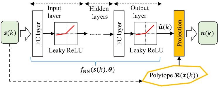
Figure 7: The DNN architecture and the projection onto ${\mathcal{R}}(\bm{x}(k))$ in (37).

We adopt a fully-connected DNN $f_{\text{NN}}(\bm{s}(k),\bm{\theta})$ in Fig. 7 to fit our samples where $\bm{s}(k)$ and $\widehat{\bm{u}}(k)$ are the input and output of the network, and $\bm{\theta}$ denotes the parameters to be trained, and the leaky rectified linear unit (ReLU) is selected as the nonlinear activation function. That is, the DNN is trained to fit the training data

$$\min\limits_{\bm{\theta}}\frac{1}{N_{\mathcal{D}}}\sum_{i=1}^{N_{\mathcal{D}}}\|f_{\text{NN}}(\bm{s}(i),\bm{\theta})-\bm{u}_{*}(i)\|^{2},$$ (36)

where $N_{\mathcal{D}}$ is the size of training dataset ${\mathcal{D}}$. We adopt the Adam stochastic gradient descent method [37] to solve (36) with PyTorch, and denote the resulting optimal solution by $\bm{\theta}_{*}$.

Note that both the sample collection and the DNN training are performed offline.

V-B The online projection and integral module to reduce tracking errors

To satisfy the state constraint in (29d) and the input limit in (29e), we further project the DNN output onto the following polytope of the feasible set

$${\mathcal{R}}(\bm{x}(k))=\left\{\bm{u}\big{|}CB_{k}\bm{u}\leq\bm{c}-CA_{k}\bm{x}(k),\bm{u}\in[0,\bar{u}]\right\}.$$ (37)

In this work, we implicitly assume that ${\mathcal{R}}(\bm{x}(k))$ is non-empty, the recursive feasibility of which has been extensively studied in the MPC theory [14]. Since ${\mathcal{R}}(\bm{x}(k))$ in (37) is the intersection of a finite number of half-spaces, $\bm{u}(k)$ can be obtained via a relatively simple QP, i.e.,

$$\bm{u}(k)=\text{argmin}_{\bm{u}}\|f_{\text{NN}}(\bm{s}(k),\bm{\theta}_{*})-\bm{u}\|^{2}$$ (38)

$$~{}~{}~{}~{}\mathrm{s.t.}~{}~{}\bm{u}\in{\mathcal{R}}(\bm{x}(k)).$$

By [38], the projection $\text{PROJ}(\bm{u},j)$ of $\bm{u}$ onto the $j$-th halfspace $C_{j}B_{k}\bm{u}\leq c-C_{j}A_{k}\bm{x}(k)$ has a closed form solution, where $C_{j}$ denotes the $j$-th row of $C$ and $c$ is given in (29d). That is

$$\text{PROJ}(\bm{u},j)=\begin{cases}\bm{u},~{}~{}~{}~{}~{}~{}~{}~{}~{}~{}~{}~{}\text{if}~{}C_{j}B_{k}\bm{u}\leq c-C_{j}A_{k}\bm{x}(k),\\ \bm{u}+\frac{\left(c-C_{j}(A_{k}\bm{x}(k)+B_{k}\bm{u})\right)B_{k}^{\text{T}}C_{j}^{\text{T}}}{\|C_{j}B_{k}\|^{2}},~{}\text{otherwise}.\end{cases}$$

Thus, the QP in (38) can be easily solved by alternating projections. As the DNN output is “close” to an optimal solution of the NLP (or QP), any infeasible DNN output is also expected close to the boundary of ${\mathcal{R}}(\bm{x}(k))$, leading to that the computational time of solving (38) is practically negligible. Instead, we can also simply use a feasible point in $\mathcal{R}(x_{k})$ as a backup.

Clearly, the approximation error of DNN depends on its size, e.g., width and depth. Since the hardware resources of the embedded chip limit the network scale, the approximation error is inevitable in implementation. In this subsection, we further introduce an IM to refine the tracking performance of the DNN-based MPC. Specifically, the constant command $r_{d}$ in Algorithm 1 is replaced by the new time-varying command

$$\widehat{r}_{d}(k)=r_{d}-c_{1}\sigma(k),~{}\sigma(k)=\sum_{i=0}^{k}\text{sat}\left(\frac{r(i)-r_{d}}{c_{2}}\right),$$ (39)

where $c_{i}$, $i\in\{1,2\}$ are positive constants and $\text{sat}(\cdot)$ is the standard saturation function [2], i.e.,

$$\text{sat}(r)=\begin{cases}1,&\text{if}~{}r>1,\\ r,&\text{if}~{}|r|\leq 1,\\ -1,&\text{if}~{}r<-1.\end{cases}$$

Unfortunately, it is impossible to provide a rigorous analysis of its impact on the stability due to the high nonlinearity and the inclusion of the DNN in the closed-loop system. We can only informally explain the function of (39). Suppose that the DNN-based MPC returns a constant steady-state tracking error $b$, i.e., $r(k)\approx r_{d}+b.$ Then, the localized motion of the closed-loop system in Fig. 7 is approximately given below

$$r(k+1)=\widehat{r}_{d}(k)+b.$$ (40)

Lemma 2

Consider the closed-loop system in (40) with a constant bias $b$. If $0<c_{2}<c_{1}<2c_{2}$, then $r(k)$ asymptotically converges to $r_{d}$.

Proof:

Substituting (39) into (40) leads to that

$$r(k+1) =r_{d}-c_{1}\sigma(k)+b$$

$$=\underbrace{r_{d}-c_{1}\sigma(k-1)+b}_{=~{}r(k)}-c_{1}\text{sat}\left(\frac{r(k)-r_{d}}{c_{2}}\right).$$ (41)

Let $\delta(k)=r(k)-r_{d}$. It follows from (V-B) that

$$\delta(k+1)=\delta(k)-c_{1}\text{sat}\left({\delta(k)}/{c_{2}}\right).$$ (42)

If $\delta(k)\geq c_{2}$, then $\text{sat}(\delta(k)/c_{2})=1$ and $\delta(k+1)=\delta(k)-c_{1}<0$, i.e., $\delta(k)$ decreases to $c_{2}$. Similarly, if $\delta(k)\leq-c_{2}$, then $\delta(k)$ increases to $-c_{2}$.

If $\delta(k)\in(-c_{2},c_{2})$, then $\text{sat}(\delta(k)/c_{2})=\delta(k)/c_{2}$ and $\delta(k+1)=(1-c_{1}/c_{2})\delta(k)$. Consider a Lyapunov function candidate $L_{3}(k)=\delta^{2}(k)$. Taking its time difference along with (42) leads to that

$$\Delta L_{3}(k)=L_{3}(k+1)-L_{3}(k)=-\frac{c_{1}}{c_{2}}\left(2-\frac{c_{1}}{c_{2}}\right)\delta(k)\leq 0.$$

By [33, Theorem 4.2], then $\delta(k)$ asymptotically converges to zero, i.e., $\lim_{k\rightarrow\infty}r(k)=r_{d}.$  

By Lemma 2, the IM in (39) aims to eliminate the steady-state range error $b$, which is also verified in Fig. 14 of Section VI-B1. However, as the PID, (39) may result in the integral windup when $\delta(k_{0})$ is very large. In practice, one can either adopt (39) only near $r_{d}$ or select a sufficiently small $c_{2}$.

V-C An easily accessible framework for the FPGA implementation

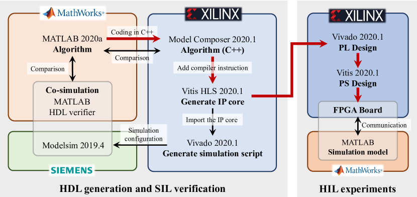
Figure 8: The HDL generation and FPGA implementation workflow.

The FPGA is good at the parallel computing, and can dramatically accelerate the evaluation of a DNN [39]. In this work, we introduce an easily accessible framework to show how to implement our tracking algorithm on an FPGA. The details are given in Fig. 8 with the hardware description language (HDL). The high-level synthesis (HLS) tool is used to convert the HL programming language for the efficient HDL code directly. The workflow of the HDL generation is described as follows.

1. Design the tracking algorithms and test them in MATLAB. In this work, they include the trajectory planning in Algorithm 1, the DNN in (36), the IM in (39), and the projection in (38).

2. Code the algorithms of Step (a) in C++ language manually, and then embed into a simulation model through the Xilinx Model Composer to confirm that the C++ code is correct.

3. Use the Vitis HLS tool to generate an IP core described in HDL from the C++ code with the compilable instructions, such as port settings, control protocol, pipeline, loop unwinding, etc.

4. Generate an IP core in verilog codes, which are then embedded into the HDL simulator (e.g. Modelsim) for correctness checking.

5. Generate the MATLAB-Modelsim co-simulation module for software-in-the-loop (SIL) simulation.

The versions of the used softwares are mentioned specifically in Fig. 8. Following Steps (a)-(e), we can confirm that the IP core correctly represents our tracking algorithms. Note that the C++ code designed in Step (b) can be directly implemented onto an embedded ARM processor for performance validation. Once the IP cores are consistent with our Matlab algorithms, we embed them into an FPGA to complete our HIL simulations.

VI HIL Simulations

In this section, we perform HIL simulations to validate the effectiveness of the proposed DNN-based MPC with an IM on an FPGA@200MHz.

VI-A The simulation setting

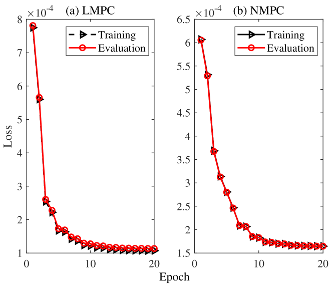
Figure 9: The mean losses during the training and evaluation process: (a) DNN-based LMPC and (b) DNN-based NMPC.

We design a fully-connected DNN with $2$ hidden layers and $100$ neurons per layer. The leaky ReLU is used with a small slope of $0.01$ as activation functions. We compare the DNN-based nonlinear and linearized MPCs on the same FPGA with $N_{p}=20$ and $N_{c}=10$. Though the offline training and online implementation of a DNN are the same for both cases, the computational cost of generating samples in the nonlinear one is much more expensive. Specifically, we have generated $10^{7}$ samples offline for each case, meaning that the number of optimization problems required to solve in each case is up to $10^{7}$, which takes $27$ hours for the linearized MPC and (estimated) $43.7$ days for the nonlinear MPC in Section IV-C. Thus, we adopt a workstation with an AMD EPYC 7742 CPU having $64$ cores to generate samples for the nonlinear MPC which takes 205 hours ($\approx 9$ days). In fact, we have tried the sample size of $5\times 10^{6}$ and unfortunately, such a sample size is not very satisfactory. Though it is beyond the scope of this work, how to increase the sample efficiency is worthy of further investigation.

Then, we pick $90\%$ of the samples for training and the rest for evaluation. Two DNNs are trained for $20$ epochs to generate the corresponding DNN-based NMPC and DNN-based LMPC and Fig. 9 shows the process of training and evaluation by using the Adam [37] with a batch size of $200$. Since the fitting losses reduce marginally after the $15$-th epoch, we regard the parameter after the $20$-th epoch as the optimal solution of (36). The training takes around $2.4$ hours on our personal computer.

VI-B The HIL simulations on an FPGA@$200$$\mathrm{M}\mathrm{H}\mathrm{z}$

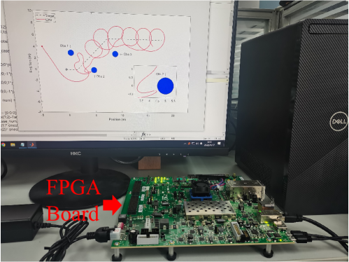
Figure 10: The Xilinx ZCU102 evaluation board.

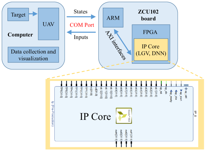
Figure 11: Schematic diagram of the HIL simulations.

FPGAs can dramatically accelerate the evaluation of DNN by its advantage in parallel processing. We introduce a framework in Fig. 8 to conveniently implement our DNN-based MPCs on an FPGA. Here we adopt the Xilinx ZCU102 as our embedded platform, which contains a Zynq UltraScale+ XCZU9EG-2FFVB1156E MPSoC. The schematic diagram of the HIL simulation is illustrated by Fig. 11, where the dynamics of the target and UAV are run on the personal computer while the LGV and DNN-based MPC are executed on the FPGA. The computer communicates with the FPGA through the COM port. Besides, an ARM Cortex-A53 processor is adopted to exchange the data between them through AXI interfaces. The digital hardware (HW) requirements of the implementation are summarized in Table IV, which shows that our method requires $9$ percent at most of the HW resources on FPGA.

Since the DNN-based NMPC and DNN-based NMPC have the same network size in this work, we use the name of DNN-based MPC to represent them for brevity. We also test the evaluation latency on the Intel Core i5 CPU, ARM, and FPGA and record the results in Table III. Interestingly, the latency on the FPGA@$200$$\mathrm{M}\mathrm{H}\mathrm{z}$ is as low as $1.26\times 10^{-4}$$\mathrm{s}$, showing its advantage of parallel computing for the DNN evaluation. Next, we examine the tracking performances of the DNN-based MPC schemes with three standoff tracking examples.

TABLE IV: A summary of the FPGA implementation

Resource	BRAM	DSP	FF	LUT
Available	1824	2520	548160	274080
Utilization	57	121	27751	23167
Utilization (%)	3.13	4.80	5.06	8.45

VI-B1 Standoff tracking of a stationary target

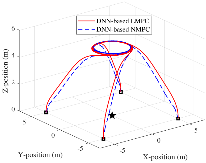
Figure 12: 3D trajectories of the UAV under DNN-based MPCs.

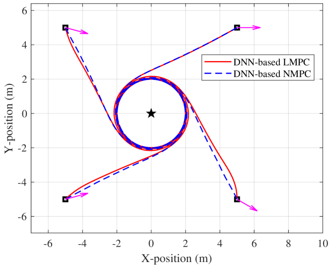
Figure 13: 2D trajectories of the UAV where squares represent its initial positions $[x_{q}(t_{0}),y_{q}(t_{0})]^{\text{T}}$ and arrows represent its initial yaw angles $\psi(t_{0})$.

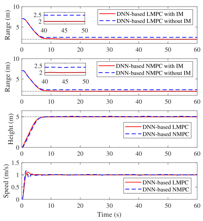
Figure 14: Relative range, height, and linear speed versus time.

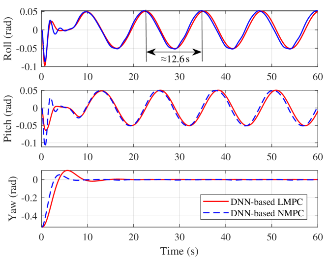
Figure 15: Euler angles of the UAV versus time.

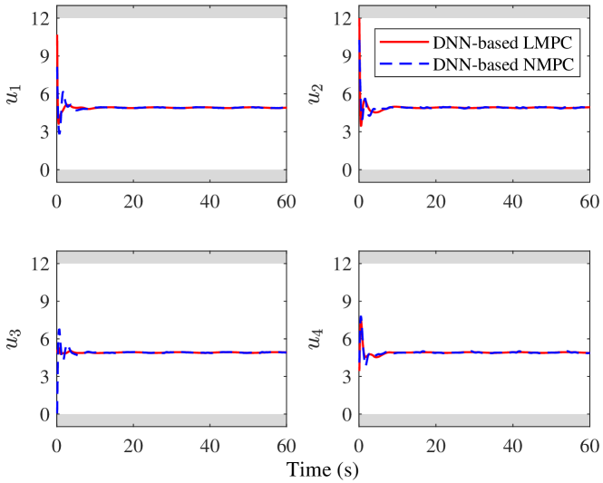
Figure 16: Control inputs to the UAV versus time.

Fixing the target at the origin, we select four different initial states for the UAV, e.g., $[x_{q}(t_{0}),y_{q}(t_{0}),\psi(t_{0})]^{\text{T}}=[5,5,0]^{\text{T}},[-5,5,-\pi/12]^{\text{T}},[-5,-5,\pi/12]^{\text{T}},[5,-5,-\pi/6]^{\text{T}}$, and set $c_{1}=1.1\cdot c_{2}=0.2$ for the IM in (39). One can observe from Figs. 12 and 13 that all trajectories converge to the desired standoff tracking. Fig. 14 further verifies that the objective in (6) is achieved from the initial state $[5,-5,-\pi/6]^{\text{T}}$ for both DNN-based MPC schemes where the desired values are marked with dotted lines.

By the partially enlarged view of Fig. 14, a significant steady-state range error occurs if we remove the IM in (39), showing its capability in refining the tracking performance. By Fig. 15, the yaw angle converges to zero in a short time from $\psi(t_{0})=-\pi/6$. However, the overshoot of the linearized one is slightly greater than that of the nonlinear counterpart. Moreover, the UAV needs to persistently adjust its roll and pitch angles at the period of $\approx 12.6$$\mathrm{s}$ to maintain the standoff tracking, which is roughly equal to the theoretical value of $\frac{2\pi r_{d}}{v_{d}}=4\pi$. Furthermore, Figs. 15 and 16 reveal that the DNN-based MPC is able to satisfy the constraints (29d) and (29e). Note that the iteration number is select as $3$ for solving (38), and the projection time via the function $\text{PROJ}(\bm{u},j)$ takes up to $6.17\upmu$$\mathrm{s}$ on the FPGA@$200$$\mathrm{M}\mathrm{H}\mathrm{z}$. This time has been included in the total computation time of $0.126$$\mathrm{m}\mathrm{s}$ in Table III.

From these results, we can easily observe that the nonlinear version indeed outperforms the linearized one in terms of tracking performance, albeit not significantly. Note that the computational cost of generating samples in the nonlinear one is much more expensive.

VI-B2 Standoff tracking of a moving target

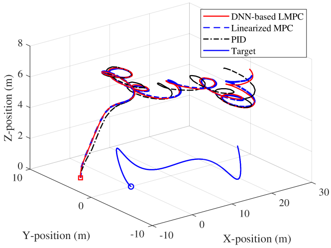
Figure 17: 3D trajectories of the UAV and target.

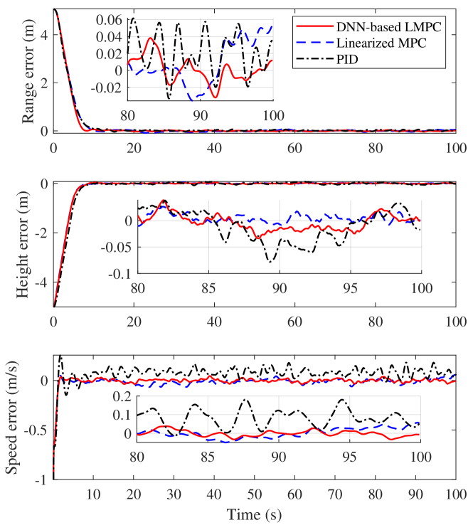
Figure 18: Tracking errors of the DNN-based LMPC, linearized MPC, and PID.

Now, we consider the moving target in Fig. 17 where its velocity is given as

$$\bm{v}_{o}(t)=[0.3\sin(0.01t+\pi/6),0.3\cos(0.06t),0.1\sin(0.15t)]^{\text{T}}$$

and add noises to the control input, e.g.,

$$\bm{u}(k)=f_{\text{NN}}(\bm{s}(k),\bm{\theta}_{*})+\bm{\omega}(k),$$

where $\bm{\omega}(k)$ is the white Gaussian noise with zero mean and variance of $0.1\cdot I_{4}$. Moreover, we compare the DNN-based linearized MPC (running on the FPGA) with (35) and the PID control [11, 12] (running on the computer). From Fig. 17, the tracking results of both the DNN-based MPC and the linearized MPC come close to each other and outperform that of the PID. Interestingly, the DNN-based MPC even has a smaller steady-state range error compared with the linearized MPC thanks to the IM in (39).

VI-B3 Standoff tracking of a moving target in the presence of obstacles

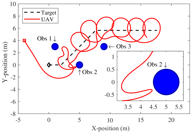
Figure 19: Trajectory of the UAV with obstacle avoidance.

Consider the standoff tracking in the presence of obstacles whose positions are assumed to be fixed and known. In this example, three circular obstacles with the radius of $0.5$$\mathrm{m}$ are included in Fig. 19. We integrate the LGV (16) with the inverse convergence vector [40] for guidance, and use the DNN-based MPC for trajectory tracking. In Fig. 19, the initial positions of the target and UAV are marked by the diamond and square, respectively, and one can observe that the standoff tracking with obstacle avoidance has completed, showing a potential application of our approach in cluttered environments.

VII Conclusion

To standoff track a moving target via a UAV, we have proposed an LGV guidance with tunable convergence rates for trajectory planning and a DNN-based MPC with an integral module for trajectory tracking. It was validated by FPGA-in-the-loop simulations that our promising improvements in the computational effort. Specifically, we have demonstrated that the proposed method represents a valid alternative to embedded implementations of MPC schemes, thus allowing its exploitation to more complex systems and applications, not limited to the one presented as test case in this paper. In the future work, we shall conduct flight tests to further validate its real-world performance.

Fei Dong received the B.S. degree from the School of Control Science and Engineering, Shandong University, Jinan, China, in 2014, the M.S. degree from the School of Instrumentation and Optoelectronic Engineering, Beihang University, Beijing, China, in 2017, and the Ph.D. degree from the Department of Automation, Tsinghua University, Beijing, China, in 2022. He is currently a Postdoctoral Researcher in the School of Automation Science and Electrical Engineering, Beihang University, Beijing, China. His research interests include model predictive control and learning-based control.

Xingchen Li received the B.S. degree from the Department of Automation, Tsinghua University, Beijing, China, in 2021. He is currently pursuing the Ph.D. degree at the Department of Automation, Tsinghua University, Beijing, China. His research interests include model predictive control and data-driven control.

Keyou You (Senior Member, IEEE) received the B.S. degree in Statistical Science from Sun Yat-sen University, Guangzhou, China, in 2007 and the Ph.D. degree in Electrical and Electronic Engineering from Nanyang Technological University (NTU), Singapore, in 2012. After briefly working as a Research Fellow at NTU, he joined Tsinghua University in Beijing, China where he is now a tenured Associate Professor in the Department of Automation. He held visiting positions at Politecnico di Torino, Hong Kong University of Science and Technology, University of Melbourne and etc. His current research interests include networked control systems, distributed optimization and learning, and their applications. Dr. You received the Guan Zhaozhi award at the 29th Chinese Control Conference in 2010, the ACA (Asian Control Association) Temasek Young Educator Award in 2019 and the first prize of Natural Science Award of the Chinese Association of Automation. He received the National Science Fund for Excellent Young Scholars in 2017, and is serving as an Associate Editor for Automatica, IEEE Transactions on Control of Network Systems, IEEE Transactions on Cybernetics, and Systems & Control Letters.

Shiji Song (Senior Member, IEEE) received the Ph.D. degree in mathematics from the Department of Mathematics, Harbin Institute of Technology, Harbin, China, in 1996. He is currently a Professor with the Department of Automation, Tsinghua University, Beijing, China. He has authored more than 180 research papers. His research interests include pattern recognition, system modeling, optimization, and control.

References

- [1] N.-M. T. Kokolakis and N. T. Koussoulas, “Robust standoff target tracking with finite-time phase separation under unknown wind,” Journal of Guidance, Control & Dynamics, vol. 44, no. 6, pp. 1183–1198, 2021.
- [2] F. Dong, K. You, and S. Song, “Target encirclement with any smooth pattern using range-based measurements,” Automatica, vol. 116, pp. 1–9, 2020.
- [3] A. S. Matveev, A. A. Semakova, and A. V. Savkin, “Tight circumnavigation of multiple moving targets based on a new method of tracking environmental boundaries,” Automatica, vol. 79, pp. 52–60, 2017.
- [4] J. O. Swartling, I. Shames, K. H. Johansson, and D. V. Dimarogonas, “Collective circumnavigation,” Unmanned Systems, vol. 2, no. 03, pp. 219–229, 2014.
- [5] D. Lawrence, “Lyapunov vector fields for UAV flock coordination,” in 2nd AIAA Unmanned Unlimited Conference, Workshop, and Exhibit, 2003.
- [6] E. W. Frew, D. A. Lawrence, and M. Steve, “Coordinated standoff tracking of moving targets using Lyapunov guidance vector fields,” Journal of Guidance Control & Dynamics, vol. 31, no. 2, pp. 290–306, 2008.
- [7] A. A. Pothen and A. Ratnoo, “Curvature-constrained Lyapunov vector field for standoff target tracking,” Journal of Guidance, Control & Dynamics, vol. 40, no. 10, pp. 2729–2736, 2017.
- [8] F. Dong, K. You, and J. Zhang, “Flight control for UAV loitering over a ground target with unknown maneuver,” IEEE Transactions on Control Systems Technology, vol. 28, no. 6, pp. 2461 – 2473, 2020.
- [9] Y. A. Kapitanyuk, A. V. Proskurnikov, and M. Cao, “A guiding vector-field algorithm for path-following control of nonholonomic mobile robots,” IEEE Transactions on Control Systems Technology, vol. 26, no. 4, pp. 1372–1385, 2018.
- [10] J. Ghommam, N. Fethalla, and M. Saad, “Quadrotor circumnavigation of an unknown moving target using camera vision-based measurements,” IET Control Theory & Applications, vol. 10, no. 15, pp. 1874–1887, 2016.
- [11] T. Luukkonen, “Modelling and control of quadcopter,” Independent research project in applied mathematics, Espoo, vol. 22, 2011.
- [12] B. Gati, “Open source autopilot for academic research-the paparazzi system,” in American Control Conference. IEEE, 2013, pp. 1478–1481.
- [13] W. Yao, H. G. de Marina, B. Lin, and M. Cao, “Singularity-free guiding vector field for robot navigation,” IEEE Transactions on Robotics, vol. 37, no. 4, pp. 1206–1221, 2021.
- [14] J. B. Rawlings, D. Q. Mayne, and M. Diehl, Model predictive control: theory, computation, and design, 2nd ed. Nob Hill Publishing Madison, WI, 2017.
- [15] A. Favato, P. G. Carlet, F. Toso, R. Torchio, and S. Bolognani, “Integral model predictive current control for synchronous motor drives,” IEEE Transactions on Power Electronics, vol. 36, no. 11, pp. 13 293–13 303, 2021.
- [16] G. Cimini, D. Bernardini, S. Levijoki, and A. Bemporad, “Embedded model predictive control with certified real-time optimization for synchronous motors,” IEEE Transactions on Control Systems Technology, vol. 29, no. 2, pp. 893–900, 2021.
- [17] M. Rubagotti, P. Patrinos, A. Guiggiani, and A. Bemporad, “Real-time model predictive control based on dual gradient projection: Theory and fixed-point FPGA implementation,” International Journal of Robust and Nonlinear Control, vol. 26, no. 15, pp. 3292–3310, 2016.
- [18] A. Bemporad, M. Morari, V. Dua, and E. N. Pistikopoulos, “The explicit linear quadratic regulator for constrained systems,” Automatica, vol. 38, no. 1, pp. 3–20, 2002.
- [19] B. Karg and S. Lucia, “Efficient representation and approximation of model predictive control laws via deep learning,” IEEE Transactions on Cybernetics, vol. 50, no. 9, pp. 3866–3878, 2020.
- [20] E. N. Hartley, J. L. Jerez, A. Suardi, J. M. Maciejowski, E. C. Kerrigan, and G. A. Constantinides, “Predictive control using an FPGA with application to aircraft control,” IEEE Transactions on Control Systems Technology, vol. 22, no. 3, pp. 1006–1017, 2014.
- [21] S. Lucia, D. Navarro, O. Lucia, P. Zometa, and R. Findeisen, “Optimized FPGA implementation of model predictive control for embedded systems using high-level synthesis tool,” IEEE transactions on industrial informatics, vol. 14, no. 1, pp. 137–145, 2017.
- [22] R. Quirynen, K. Berntorp, and S. Di Cairano, “Embedded optimization algorithms for steering in autonomous vehicles based on nonlinear model predictive control,” in American Control Conference. IEEE, 2018, pp. 3251–3256.
- [23] F. Xu, Z. Guo, H. Chen, D. Ji, and T. Qu, “A custom parallel hardware architecture of nonlinear model predictive control on FPGA,” IEEE Transactions on Industrial Electronics, vol. 69, no. 11, pp. 11 569–11 579, 2022.
- [24] X. Zhang, M. Bujarbaruah, and F. Borrelli, “Near-optimal rapid MPC using neural networks: A primal-dual policy learning framework,” IEEE Transactions on Control Systems Technology, vol. 29, no. 5, pp. 2102–2114, 2021.
- [25] S. Lucia, D. Navarro, B. Karg, H. Sarnago, and O. Lucia, “Deep learning-based model predictive control for resonant power converters,” IEEE Transactions on Industrial Informatics, vol. 17, no. 1, pp. 409–420, 2021.
- [26] M. Abu-Ali, F. Berkel, M. Manderla, S. Reimann, R. Kennel, and M. Abdelrahem, “Deep learning-based long-horizon MPC: Robust, high performing and computationally efficient control for PMSM drives,” IEEE Transactions on Power Electronics, vol. 37, no. 10, pp. 12 486–12 501, 2022.
- [27] A. Tagliabue, D.-K. Kim, M. Everett, and J. P. How, “Efficient guided policy search via imitation of robust tube MPC,” in International Conference on Robotics and Automation. IEEE, 2022, pp. 462–468.
- [28] S. W. Chen, T. Wang, N. Atanasov, V. Kumar, and M. Morari, “Large scale model predictive control with neural networks and primal active sets,” Automatica, vol. 135, pp. 1–9, 2022.
- [29] K. J. Chan, J. A. Paulson, and A. Mesbah, “Deep learning-based approximate nonlinear model predictive control with offset-free tracking for embedded applications,” in American Control Conference. IEEE, 2021, pp. 3475–3481.
- [30] F. Dong, X. Li, K. You, and S. Song, “Deep neural network based model predictive control for standoff tracking by a quadrotor UAV,” in IEEE Conference on Decision and Control. IEEE, 2022, accepted.
- [31] MathWorks, “Control of quadrotor using nonlinear model predictive control,” 2021. [Online]. Available: https://www.mathworks.com/help/mpc/ug/control-of-quadrotor-using-nonlinear-model-predictive-control.html
- [32] F. Dong and K. You, “The isoline tracking in unknown scalar fields with concentration feedback,” Automatica, vol. 133, pp. 1–9, 2021.
- [33] H. K. Khalil, Nonlinear Systems, 3rd ed. Upper Saddle River, NJ, USA: Prentice Hall, 2002.
- [34] A. S. Matveev, H. Teimoori, and A. V. Savkin, “Range-only measurements based target following for wheeled mobile robots,” Automatica, vol. 47, no. 1, pp. 177–184, 2011.
- [35] S. Gros, M. Zanon, R. Quirynen, A. Bemporad, and M. Diehl, “From linear to nonlinear MPC: Bridging the gap via the real-time iteration,” International Journal of Control, vol. 93, no. 1, pp. 62–80, 2020.
- [36] A. Domahidi, A. U. Zgraggen, M. N. Zeilinger, M. Morari, and C. N. Jones, “Efficient interior point methods for multistage problems arising in receding horizon control,” in IEEE conference on decision and control. IEEE, 2012, pp. 668–674.
- [37] D. P. Kingma and J. Ba, “Adam: A method for stochastic optimization,” arXiv preprint, arXiv:1412.6980, 2014.
- [38] S. Chen, K. Saulnier, N. Atanasov, D. D. Lee, V. Kumar, G. J. Pappas, and M. Morari, “Approximating explicit model predictive control using constrained neural networks,” in American control conference. IEEE, 2018, pp. 1520–1527.
- [39] J. Nadales, J. Manzano, A. Barriga, and D. Limon, “Efficient FPGA parallelization of Lipschitz interpolation for real-time decision-making,” IEEE Transactions on Control Systems Technology, vol. 30, no. 5, pp. 2163–2175, 2022.
- [40] J. Wilhelm, G. Clem, D. Casbeer, and A. Gerlach, “Circumnavigation and obstacle avoidance guidance for UAVs using gradient vector fields,” in AIAA Scitech 2019 Forum, 2019, pp. 1–13.