DeepGlow: an efficient neural-network emulator of physical afterglow models for gamma-ray bursts and gravitational-wave events

Abstract

Gamma-ray bursts (GRBs) and double neutron-star merger gravitational wave events are followed by afterglows that shine from X-rays to radio, and these broadband transients are generally interpreted using analytical models. Such models are relatively fast to execute, and thus easily allow estimates of the energy and geometry parameters of the blast wave, through many trial-and-error model calculations. One problem, however, is that such analytical models do not capture the underlying physical processes as well as more realistic relativistic numerical hydrodynamic (RHD) simulations do. Ideally, those simulations are used for parameter estimation instead, but their computational cost makes this intractable. To this end, we present DeepGlow, a highly efficient neural network architecture trained to emulate a computationally costly RHD-based model of GRB afterglows, to within a few percent accuracy. As a first scientific application, we compare both the emulator and a different analytical model calibrated to RHD simulations, to estimate the parameters of a broadband GRB afterglow. We find consistent results between these two models, and also give further evidence for a stellar wind progenitor environment around this GRB source. DeepGlow fuses simulations that are otherwise too complex to execute over all parameters, to real broadband data of current and future GRB afterglows.

ASTRON, the Netherlands Institute for Radio Astronomy, Oude Hoogeveensedijk 4,7991 PD Dwingeloo, The Netherlands O. M. Boersma]o.m.boersma@uva.nl dd Mmm YYYY

1 INTRODUCTION

Bright, distant sources such as Active Galactic Nuclei and Gamma-ray bursts (GRBs) that are variable or transient, are powered by relativistic blast waves (Blandford & McKee, 1976). Following the detection of the first GRB afterglow  (GRB970228; Costa et al., 1997), modeling of these expanding explosions has been given great attention in the literature. The recent detection of the short gamma-ray burst GRB170817A (e.g., Abbott et al., 2017a) coincident with the gravitational-wave detection of binary neutron star merger GW170817 (Abbott et al., 2017b), and the subsequent detection of a multi-frequency afterglow (e.g. Chornock et al., 2017; Coulter et al., 2017; Alexander et al., 2017; Haggard et al., 2017; Hallinan et al., 2017) have further heightened this interest in detecting afterglows (e.g. Boersma et al., 2021).

As the afterglows are now known to produce radio, optical and X-ray emission, various (semi-)analytical models have been developed to analyze this broadband data (Wijers et al., 1997; Sari et al., 1998; Granot & Sari, 2002; Leventis et al., 2012; Ryan et al., 2020). Such analytical models are relatively fast to execute and are thus easily applicable in parameter estimation studies where the model needs to be calculated many times over (e.g., Panaitescu & Kumar 2002). These models do not fully capture the physical processes, however, encompassed in more realistic relativistic hydrodynamical (RHD) simulation approaches like BOXFIT (van Eerten et al., 2012). BOXFIT is built on top of a series of 2D RHD jet simulations which describe the dynamics of the afterglow. BOXFIT then interpolates between the output of these simulations, saved in a large number of compressed snapshots at fixed times, and applies a linear radiative transfer approach to calculate spectra and light curves. This method works partly because of the scale invariance of jets with different energies or densities, as demonstrated in van Eerten et al. (2012). This makes it possible to compute the afterglow for arbitrary energy and densities from the saved simulation snapshots with specific energy and density. To calculate the afterglow flux, it is assumed that the dominant radiation is synchrotron radiation. The jet fluid, computed in the RHD simulations, is divided into small cells for which the broadband synchrotron emission is calculated. A large number of rays are passed through these fluid cells and the observed flux is obtained by integrating the emission over these rays using the linear radiative transfer equation (Van Eerten et al., 2010) for each ray. While BOXFIT has been used to characterize GRB afterglow data (e.g., Higgins et al. 2019), its computational cost makes it an unattractive, resource- and energy-heavy approach for studies that, e.g., fit a large population of GRB afterglow data using sophisticated methods (Aksulu et al., 2022), or simulate large numbers of afterglows to forecast how to infer binary and fireball parameters from future gravitational-wave and electromagnetic detections (Boersma & van Leeuwen, 2022).

In recent years, the use of machine learning techniques has exploded across the (astronomical) sciences to speed up various processes with high computational complexity (e.g., Schmit & Pritchard 2018; Kasim et al. 2021; Kerzendorf et al. 2021). Specifically, deep learning and neural network (NN) methods have been used extensively owing to their ability to accurately replicate highly non-linear relations between input and output data (e.g., Hornik et al. 1989; Cybenko 1989). Furthermore, after training the NNs, they are usually quick to execute because only a relative small number of computational steps need to be performed, if they are not too large. This is further aided by the existence of optimized deep learning libraries like TensorFlow.

In this work, we use NNs to emulate the output of BOXFIT with small evaluation cost compared to running BOXFIT itself. We emulate both interstellar medium (ISM) and stellar wind like progenitor environments. We verify the accuracy of our NNs by comparing the output to real BOXFIT data and then test their validity by inferring the properties of the afterglow of GRB970508 (e.g., Panaitescu & Kumar 2002; Yost et al. 2003) which has a large broadband dataset. We compare the results to a recent analytical model calibrated to BOXFIT simulation data (Ryan et al. 2015, Ryan et al. in prep). The trained NNs are freely available in the DeepGlow Python package and all code associated with the methodology in this work is present as well.

In Section 2, we describe the methods used to generate the BOXFIT output training data and how we trained the NNs. We demonstrate the accuracy of DeepGlow in Section 3 and fit the broadband dataset of GRB970508 as a test case in Section 4. We conclude and look towards the future in Sections 5 and 6.

2 METHODS

2.1 Training data

Table 1: GRB afterglow parameter distributions used to generate the training data.

Parameter		Distribution	Range
$\theta_{0}$	(jet half angle)	Log-Uniform	$(0.01,0.5\pi)$ rad
$E_{\mathrm{K,iso}}$	(explosion energy)	Log-Uniform	$(10^{50},10^{56})$ ergs
$n_{\mathrm{ref}}$	(density)	Log-Uniform	$(10^{-5},10^{3})$ $\mathrm{cm}^{-3}$
$\theta_{\mathrm{obs}}$	(observer angle)	Uniform	$(0.01,2\times\theta_{0})$ rad
$p$	(power-law index)	Uniform	$(2,3)$
$\epsilon_{B}$	(magnetic energy fraction)	Log-Uniform	$(10^{-10},1)$
$\epsilon_{e}$	(electron energy fraction)	Log-Uniform	$(10^{-10},1)$
$\nu_{\mathrm{obs}}$	(observer frequency)	Log-Uniform	$(10^{8},10^{19})$ Hz
$t_{\mathrm{obs}}$	(observer time)	Fixed	$0.1$ d - $1000$ d
$\xi_{N}$	(acc. electrons fraction)	Fixed	$1$
$d_{L}$	(luminosity distance)	Fixed	$50$ Mpc
$z$	(redshift)	Fixed	$0$

Several sets of simulation data are available to be used with BOXFIT. These differ in the progenitor environment and the Lorentz frame used to do the simulations. We used two sets of simulation data in this work, the ”lab frame ISM environment” set and the ”medium boost wind environment” set, and generated two corresponding sets of training data consisting of 200 000 light curves each. We employed the computing cluster of the Apertif Radio Transient System (van Leeuwen et al., 2023) using 40 nodes each having 40 CPU cores. Generating the datasets took around a hundred thousand combined core hours.

To generate light curves with BOXFIT, ten GRB afterglow parameters must be specified: (i) the jet half opening angle $\theta_{0}$ in radians; (ii) the isotropic-equivalent explosion energy $E_{\mathrm{K,iso}}$ in ergs; (iii) the circumburst number density $n_{\mathrm{ref}}$ in $\mathrm{cm}^{-3}$; (iv) the observer angle $\theta_{\mathrm{obs}}$ in radians; (v) the index of the synchrotron power law slope of the accelerated electrons $p$; (vi) the fraction of thermal energy in the magnetic fields $\epsilon_{B}$; (vii) the fraction of thermal energy in the accelerated electrons $\epsilon_{e}$; (viii) the fraction of accelerated electrons $\xi_{N}$; (ix) the observer luminosity distance $d_{L}$ in cm; and (x) the cosmic redshift $z$. As the GRB afterglow flux scales straightforwardly with $\xi_{N}$, $d_{L}$, and $z$, we fixed those parameters to, in principle arbitrary, values of $1$, $50$ Mpc, and 0, respectively, when generating the training data. We chose the remaining parameters from broad log-uniform distributions except for $p$ which was uniformly distributed and $\theta_{\mathrm{obs}}$ which was distributed uniformly as well with a maximum $\theta_{\mathrm{obs}}<2\times\theta_{0}$. The parameter distributions are summarized in Table 1.

We generated the light curves on a fixed observer time grid between $t_{\mathrm{obs},0}=0.1$ days and $t_{\mathrm{obs,1}}=1000$ days with 117 observer data points. The amount of observer data points chosen is a trade-off between the time it takes to generate the training data and the resolution of the resulting light curves.

For 32% (ISM environment) to 44% (wind environment) of the generated light curves, the BOXFIT calculations did not cover the entire observer time range which resulted in zero flux values at observer times with no coverage. In Fig. 1, we show the fraction of zero flux values as a function of observer time. The flux at a certain observer time corresponds to the combined emission from a range of emission times (van Eerten et al., 2012). If these times are not captured in the RHD simulations incorporated into BOXFIT, BOXFIT uses the Blandford–McKee (BM) solution (Blandford & McKee, 1976) at early times as a starting point, beginning with a fluid Lorentz factor of 300. Still, very early observer epochs are sometimes not covered by this BM solution either, because the thin shell of the shock at that time is not numerically resolved, or because the emission times occur before our asymptotic BM limit of Lorentz factor 300. For such observer times either the flux computed by BOXFIT is zero, or it rapidly drops off as only some of the emission times which are summed up can be calculated. For afterglow measurements of GRBs at such early times, BOXFIT, and by extension DeepGlow, is not a suitable model and should not be used. Furthermore, in the first few hours of GRB afterglow Swift (Gehrels et al., 2004) data often a plateau phase is observed (e.g. Nousek et al. 2006), possibly due to a coasting or extended energy injection phase. These are not modeled in BOXFIT. Still, these afterglows will eventually evolve to a regime where BOXFIT is valid. It is also possible that very late observer times cannot be calculated by the BOXFIT simulations or the BM solution. In general, the broadband GRB afterglow datasets we are interested in modeling have measurements in the BOXFIT validity regime and the incomplete coverage is thus not an issue. Still, this does have an effect on the performance of DeepGlow as we will show in Section 3. Overall, care must be taken when training the NNs on light curves with zero flux values and we return to this point in Section 2.2.

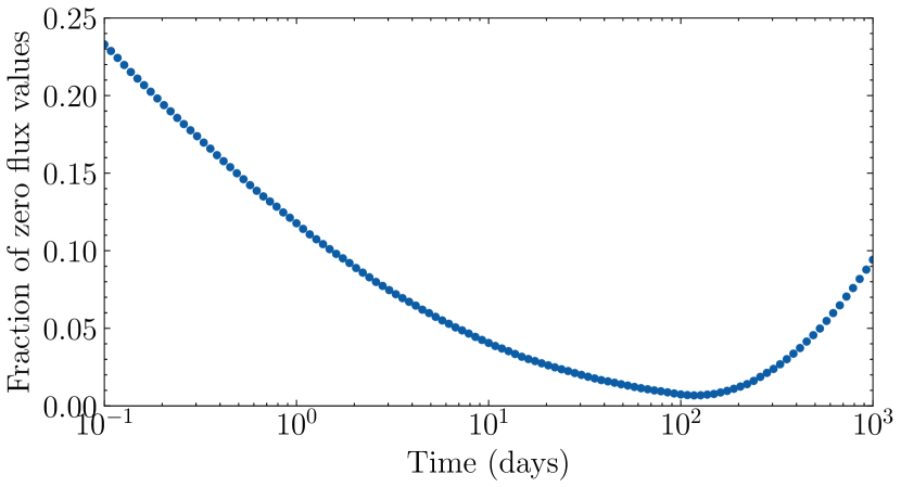
Figure 1: The fraction of light curves where the flux at a certain observer time is set to zero by BOXFIT when generating the training data. The dots correspond to the 117 datapoints generated for each light curve.

We did not use a fixed grid of observer frequencies but chose a random $\nu_{\mathrm{obs}}$ for each light curve from a log-uniform distribution similar to the GRB afterglow parameters mentioned above. We picked a broad range in observer frequencies from $\nu_{0}\ =\ 10^{8}$ Hz to $\nu_{1}\ =\ 10^{19}$ Hz such that the trained NNs can be used to fit most broadband GRB afterglow datasets.

Various resolution and radiation related parameters must be specified in BOXFIT which we left mostly to their default settings. We did adjust three parameters pertaining to the numerical resolution of the radiative transfer calculations in BOXFIT. More specifically, these three parameters correspond to (i,ii) the number of rays used in the radiative transfer steps in the radial and tangential direction; and (iii) the total number of simulation snapshots used. The first two parameters determine the number of rays for which the flux is calculated, while the third parameter sets the resolution along the rays. We set these to $500,\ 30,$ and $500$, respectively, which are lower values than the default settings, and this is again a trade-off between computing time and the quality of the light curve. From our testing, the numerical noise of the light curves with the mentioned values is similar to that of the default settings while saving about half of the computation time.

2.2 Neural Network setup and training

Each sample in our training data consists of eight input values ($\theta_{0}$, $E$, $n$, $p$, $\epsilon_{B}$, $\epsilon_{e}$, $\theta_{\mathrm{obs}}$ and $\nu_{\mathrm{obs}}$) and 117 output values corresponding to the observer data points. As a preprocessing step, we took the $\log_{10}$ of the input and output values (except for $p$ which has a limited range) and removed the mean and variance. GRB afterglow light curves generally follow a power-law decay (e.g., Sari et al. 1998), thus the flux values at early observer times can be orders of magnitude larger than at late observer times. Taking the $\log_{10}$ of the flux values is a necessary step for the early time bins not to dominate the objective (loss) function for NN training. In log-space we used the StandardScaler in the scikit-learn Python package (Pedregosa et al., 2011) to standardize the individual time bins by subtracting the mean of the flux values and scaling to unit variance. The same steps were done for the input parameters. We also experimented with the MinMaxScaler but found this to produce slightly worse results.

We modeled the relation between the resulting input and output values using a feed-forward NN (see e.g., Schmidhuber 2015, for an overview) in Keras/Tensorflow 2.9.1. One NN was trained for each of the two progenitor environments. The best architecture and hyperparameters of the NNs were obtained through a trial-and-error approach, i.e. manually searching the hyperparameter space. While, in the limit of finite training data, the reproduction will not be perfect, we aimed for DeepGlow to reproduce BOXFIT with an error which is generally well below the typical fractional GRB afterglow flux measurement error ($\approx 10-30\%$ in the GRB970508 dataset). We experimented with the number of layers, the size of the layers, learning rate, activation function and batch size. Three large hidden layers consisting of 1000 neurons with a softplus activation function produced the best results. The output layer, consisting of 117 neurons, uses a linear activation function. We used Nesterov-adam (Sutskever et al., 2013) as the optimizer with a cyclic learning rate (triangular2 policy, Smith 2015) between $10^{-4}$ and $10^{-2}$. We employed 90% of the training data to actually train the network, the remaining 10% was used to the test the accuracy of the NNs afterwards. The data was fed through the network with a batch size of 128 for 2000 epochs and we selected the realization with the highest accuracy, i.e. lowest median fractional error compared to BOXFIT over the test dataset, from all epochs. In general, three to five equally-sized hidden layers with at least 200 neurons brought the reproduction error into our goal range. A cyclic learning rate schedule was also crucial in bringing the error down. Changing the activation function or the batch size had limited influence, however. We did not experiment with different optimizers.

NNs run the risk of overfitting on the training data and not generalizing well to unseen test data (e.g., Caruana et al. 2000; Ying 2019). Because of the uniform way in which the light curve data was generated through our Monte Carlo approach and the relatively large size of the training and test data, the risk of overfitting is low in our case. For reference, we compare the performance of the trained NNs on both the test dataset and training dataset in A, where we show these are almost the same.

We chose the mean absolute error as our loss function; using the mean squared error loss resulted in reproduction errors an order of magnitude worse. As mentioned in Section 2.1, not all light curves have nonzero flux values at each of the 117 data points. Naively computing the loss for these light curves gives a numerical error as the $\log_{10}0=-\infty$. Removing these light curves entirely from the training data would prohibit the NNs from learning the parts of the light curves which do have calculated flux values, which is not ideal. Thus, we modified the loss function such that it disregards these missing values. The expression for the loss function for a batch becomes:

$$\text{MAE}(\textbf{y}{\text{true}},\textbf{y}{\text{pred}})=\frac{1}{N}\sum_{i=1}^{B}\sum_{j=1}^{T}w_{ij}|y_{ij,\text{true}}-y_{ij,\text{pred}}|$$ (1)

$$w_{ij}=\begin{cases}0,&\text{if}\ y_{ij,\text{true}}=0\\ 1,&\text{otherwise}\end{cases}$$ (2)

$$N=\sum_{i=1}^{B}\sum_{j=1}^{T}w_{ij}$$ (3)

Here, ytrue and ypred represent the true and predicted flux values, respectively. $B$ is the batch size (128), and $T$ is the number of time bins (117). The index $i$ iterates over the light curves in the batch, and the index $j$ iterates over the time bins. The variable $w_{ij}$ is a weight that determines whether a specific element contributes to the loss function, and $N$ is the total number of non-zero elements in the batch.

The NNs then only train on parts of the light curves with nonzero flux values. Importantly, this does not mean that the NNs learn to output zero at the zero flux values in the training data. Instead, they will learn to extrapolate the flux to these regions based on the light curves that do have complete coverage. This method is perhaps less physically motivated than, for example, using closure relations (see e.g, Gao et al. 2013) to fill in the zero flux gaps. It does rely only on the BOXFIT calculations, however, and is straightforward to implement in the NN training procedure.

3 DEEPGLOW RESULTS

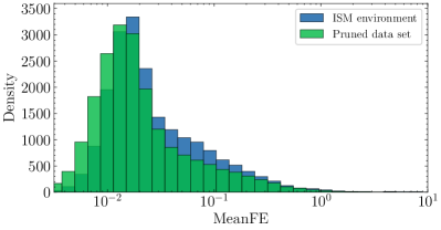
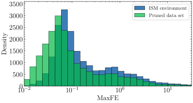
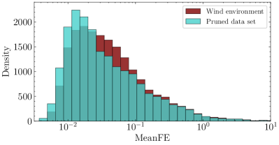
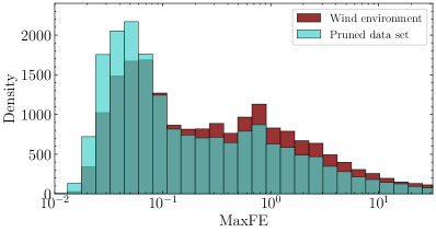
Figure 2: MeanFE and MaxFE distributions scaled logarithmically on the horizontal axis of the light curves in our test dataset. The upper two panels show these distributions assuming an ISM progenitor environment while a wind progenitor environment is used in the lower two panels. In each panel, the pruned dataset refers to the distributions calculated over a smaller observer time range starting from $t\ \approx\ 1$ day.

During the training stage of the NNs we calculated the median fractional error over all flux values in the test dataset at the same time to gauge the accuracy of DeepGlow. To get a more complete picture of how well it performs in a production setting, we followed a similar approach to Kerzendorf et al. (2021) and defined for each light curve in our test dataset:

$$\mathrm{MeanFE} =\frac{1}{N}\sum_{i=1}^{N}\frac{|d^{DG}_{k,i}-d^{BF}_{k,i}|}{d^{BF}_{k,i}},$$ (4)

$$\mathrm{MaxFE} =\mathrm{Max}_{i=1}^{N}\frac{|d^{DG}_{k,i}-d^{BF}_{k,i}|}{d^{BF}_{k,i}},$$ (5)

with $N\ (\ =\ 117)$ the amount of data points, and $d_{k,i}$ the flux value of the $i$-th data point of the $k$-th light curve in our test dataset generated by either DeepGlow or BOXFIT.

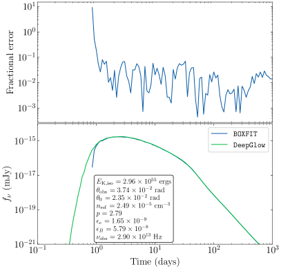
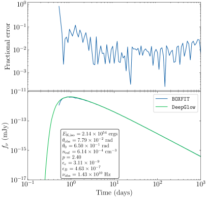
Figure 3: Examples of light curves in the test data sets where the $\mathrm{MaxFE}$ is concentrated at the edge of the observer times which are still covered by BOXFIT calculations. The left panel shows an example for the ISM environment whereas the right panel shows an example for the wind environment. In both panels, the top plot shows the fractional error of the DeepGlow prediction versus the BOXFIT calculations, whereas the bottom plot shows both the BOXFIT (blue) and DeepGlow (green) light curves. The inset shows the corresponding parameter values.

For each progenitor environment, we calculated the $\mathrm{MeanFE}$ and $\mathrm{MaxFE}$ distributions over the test dataset for the full observer time range. In addition, we also calculated these statistics assuming a more limited range starting from $t_{\mathrm{obs}}\ \approx\ 1$ day ($i\ =\ 30$), after which most GRB afterglow observations usually take place. We will refer to this second case as the pruned dataset which has the same amount of light curves as the test dataset but takes fewer flux values into consideration. Both distributions, the $\mathrm{MeanFE}$ and $\mathrm{MaxFE}$ statistics calculated over the full test dataset and the pruned dataset, are shown in Figure 2, scaled logarithmically on the horizontal axis. The median of each $\mathrm{MeanFE}$ and $\mathrm{MaxFE}$ distribution shown is given in Table 2.

Median values	ISM environment	Wind environment
$\mathrm{MeanFE}$	0.020	0.034
$\mathrm{MeanFE}$ pruned dataset	0.016	0.026
$\mathrm{MaxFE}$	0.104	0.228
$\mathrm{MaxFE}$ pruned dataset	0.062	0.099

Table 2: Median values of the MeanFE and MaxFE distributions for each progenitor environment.

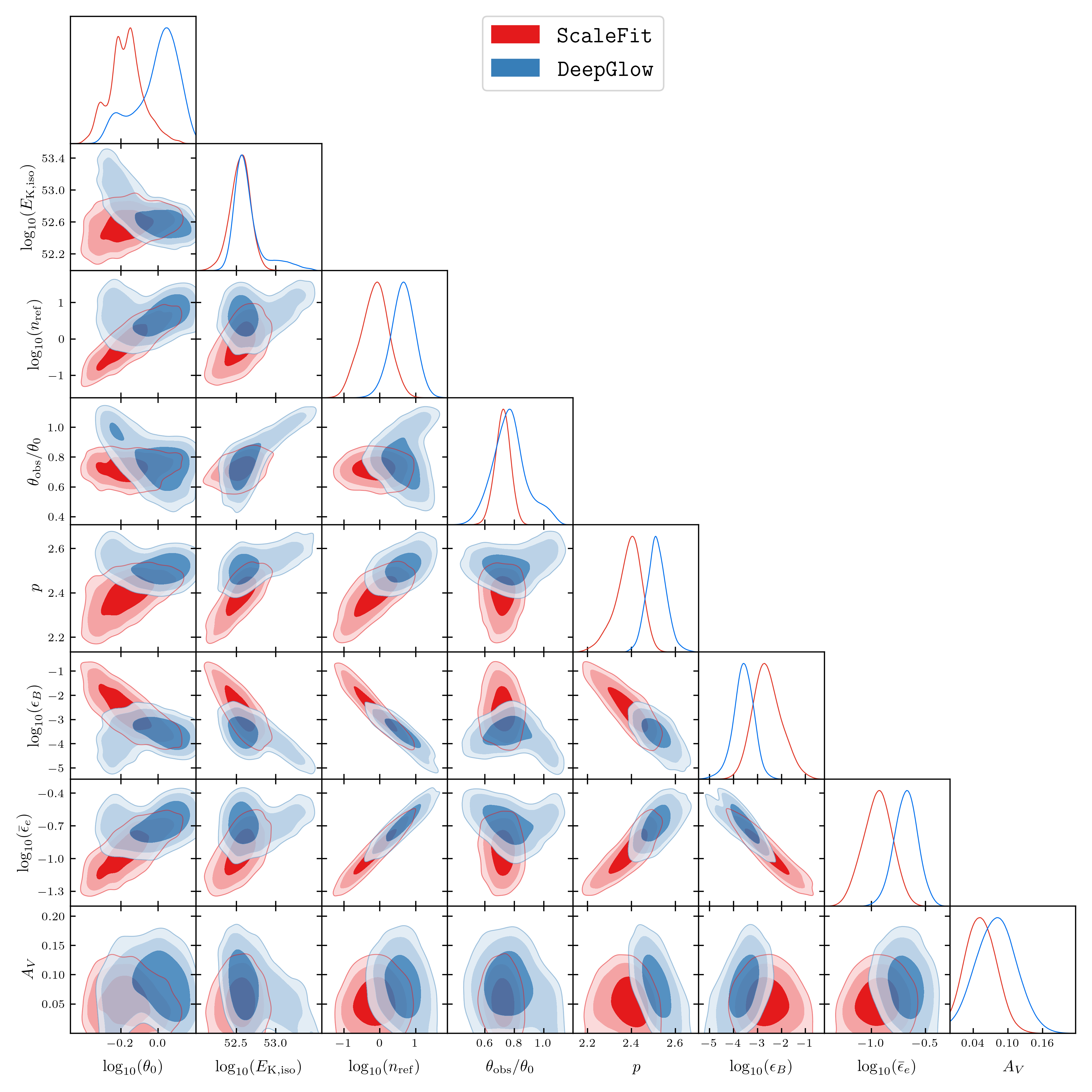
Figure 4: Posterior distribution of the GRB afterglow parameters for GRB970508 assuming an ISM progenitor environment. The likelihood was calculated using either the ScaleFit model in red or our DeepGlow model in blue.

In general, the average NN reproduction error per light curve, i.e. $\mathrm{MeanFE}$, is a few percent which is well below the typical measurement error on GRB afterglow observations. For the ISM environment, the $\mathrm{MaxFE}$ on most generated light curves is smaller than the typical measurement error as well, certainly when looking at the pruned dataset. The $\mathrm{MaxFE}$ in the wind environment case can become quite high ($>30\%$) but this improves considerably in the pruned dataset. The better performance in the pruned dataset can be traced back to better BOXFIT calculation coverage for later observer times, see Fig. 1. There are fewer data points to train on at $t_{\mathrm{obs}}<1$ days, and the flux evolution is more sporadic, making it harder to predict. We observe that the average $\mathrm{MaxFE}$ is substantially higher for light curves where the BOXFIT coverage is incomplete. At the limits of the observer times which still have nonzero fluxes for these light curves, the simulated BOXFIT flux can drop off very rapidly and/or have large simulation noise. As mentioned in Section 2.1, this is also a sign of incomplete simulation coverage even though the flux is still nonzero. Slight errors in e.g. the reproduced slope by DeepGlow can easily lead to large fractional errors compared to BOXFIT in these instances. We show two examples of this for light curves in our test dataset in Fig. 3. Thus, large fractional errors and data points with zero fluxes are usually in close proximity with one another with respect to their observer times. Consequently, $\mathrm{maxFE}$ errors are often found in regions where BOXFIT calculations are intrinsically inaccurate and NN emulation is not meaningful anyways. Because the BOXFIT coverage is less of an issue in the pruned dataset, the median $\mathrm{MaxFE}$ will also be lower.

Incomplete BOXFIT coverage is more likely in quite extreme regions of the GRB afterglow parameter space (e.g. very high energies in combination with very low densities) which may not be where most observed GRB afterglows reside. Still, for the wind environment in particular, it is possible that the reproduction error will lead to a significant systematic error contribution compared to BOXFIT when fitting some observed data points. Moreover, while DeepGlow is trained on light curves with a fixed observer time grid, we use linear interpolation to allow for arbitrary observer times within the limits $t_{0}$ and $t_{1}$. This could also be an extra source of systematics not captured in the $\mathrm{MeanFE}$ and $\mathrm{MaxFE}$ distributions.

For many GRB afterglow datasets, we are confident that DeepGlow can be used to fit the data in place of BOXFIT with good accuracy. We advise caution, however, when interpreting GRB afterglow datasets with best fit parameter values which lie in regions of the parameter space where BOXFIT has incomplete coverage over the observation times of the measurements.

The mean and standard deviation of the DeepGlow evaluation time are just $2.2\pm 0.2$ ms on a single thread of our computing cluster. In contrast, the BOXFIT mean and standard deviation evaluation time on 40 threads of a single node are $29.6\pm 4.6$ s. DeepGlow thus represents an approximate $10^{4}$ factor speedup in evaluation, which further increases if less threads for BOXFIT parallel execution are available, making parameter estimation with the physics of BOXFIT possible.

In the next section, we will use DeepGlow to estimate the parameters of the GRB970508 afterglow. In A, we provide some additional figures related to the training of the NNs.

4 TEST CASE: GRB970508

4.1 Gaussian Process framework

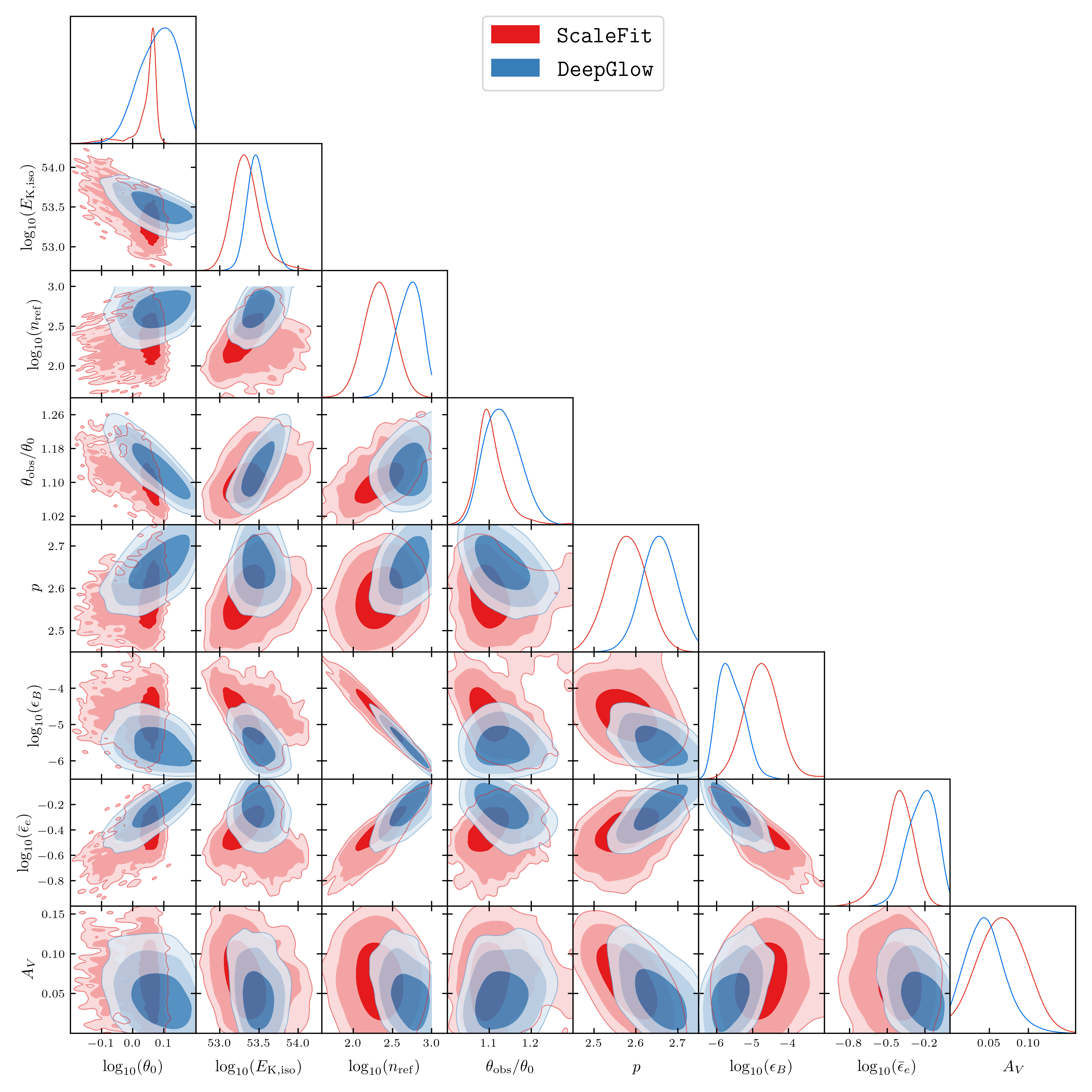
Figure 5: Same as Figure 4, except now assuming a wind progenitor environment.

As a first scientific application of DeepGlow, we inferred the properties of the afterglow of GRB970508 using the methods in Aksulu et al. (2022, hereafter referred to as A22). They build on the methods in Aksulu et al. (2020) and use a Gaussian Process (GP, Rasmussen & Williams 2006) framework to estimate the parameters of GRB afterglow datasets while allowing for unknown systematics to be modeled simultaneously as well. Especially when considering unmodeled systematic effects such as scintillation at radio frequencies, conventional $\chi^{2}$ fitting methods can lead to underestimated uncertainties on parameters (Aksulu et al., 2020). By modeling the systematics using GPs, we have a much more robust method to obtain parameter estimates. In A22, the GRB afterglow model of choice is ScaleFit (Ryan et al. 2015, Ryan et al. in prep). It is a semi-analytical model which uses pre-calculated spectral tables from BOXFIT to model the GRB afterglow in different spectral regimes. ScaleFit is a computationally inexpensive alternative to BOXFIT and, also in contrast to BOXFIT, is valid in all spectral regimes (see A22 for details). A downside to ScaleFit is the assumptions it has to make about the sharpness of spectra around break frequencies. This follows naturally from the radiative transfer approach that BOXFIT uses and is thus incorporated in DeepGlow too. The evaluation time for ScaleFit, after generating the necessary spectral tables, is 0.9 $\pm$ 0.1 ms on our computing cluster. Taking into account the sampling overhead, parameter estimation runs are similar in runtime to those with DeepGlow.

A22 use the MultiNest nested sampler (Feroz et al., 2009) through the Python implementation PyMultiNest (Buchner et al., 2014) to sample the GP likelihood (Eq. 2 of Aksulu et al. 2020). This nested sampling approach requires on the order of 100 000 likelihood evaluations for each fit. Because BOXFIT can generate a light curve for only one frequency at a time, and the GRB970508 observations cover twelve different frequencies, BOXFIT would have to be run twelve times for one likelihood evaluation. This becomes intractable to calculate, certainly on a repeated basis when, e.g., fitting an afterglow dataset multiple times with different MultiNest settings. We thus compared the results using DeepGlow to the results of A22 using ScaleFit. While this is not a direct comparison between DeepGlow and BOXFIT, ScaleFit is similar enough to BOXFIT to give a general indication of how well DeepGlow works in practice. We performed two fits per afterglow model, one for each progenitor environment.

An important difference between DeepGlow and ScaleFit lies in how the model parameters $p$ and $\epsilon_{e}$ are handled. ScaleFit fits the parameter $\bar{\epsilon}_{e}\equiv\frac{p-2}{p-1}\epsilon_{e}$ instead of $\epsilon_{e}$ to allow for fits with $p\ <\ 2$. For the sake of comparison, we also fitted $\bar{\epsilon}_{e}$ and calculated $\epsilon_{e}$ from $\bar{\epsilon}_{e}$. A22 extended the prior range of $p$ below two as well. This is not possible for DeepGlow as BOXFIT, on which it is trained, cannot calculate light curves or spectra with $p\ <\ 2$. Here we are thus limited to fits with $p\ >\ 2$ which might hamper any comparisons. The posteriors of GRB970508 using ScaleFit have little support for $p\ <\ 2$, however, and we assume that our more limited prior range did not influence the results much in this case (though it might for other GRB afterglows which do have support for $p\ <\ 2$, see A22). The rest of the methodology, including the prior ranges and MultiNest settings, was the same as those in A22. As such, we also included $A_{V}$, the rest-frame value for host galaxy dust extinction, as a free parameter in the model.

We will limit ourselves to quantitative comparisons between the two afterglow models in the next section. An in-depth comparison of the differences in estimated parameters that may arise in relation to any physical differences between DeepGlow, i.e. BOXFIT, and ScaleFit is beyond the scope of this work.

4.2 Results

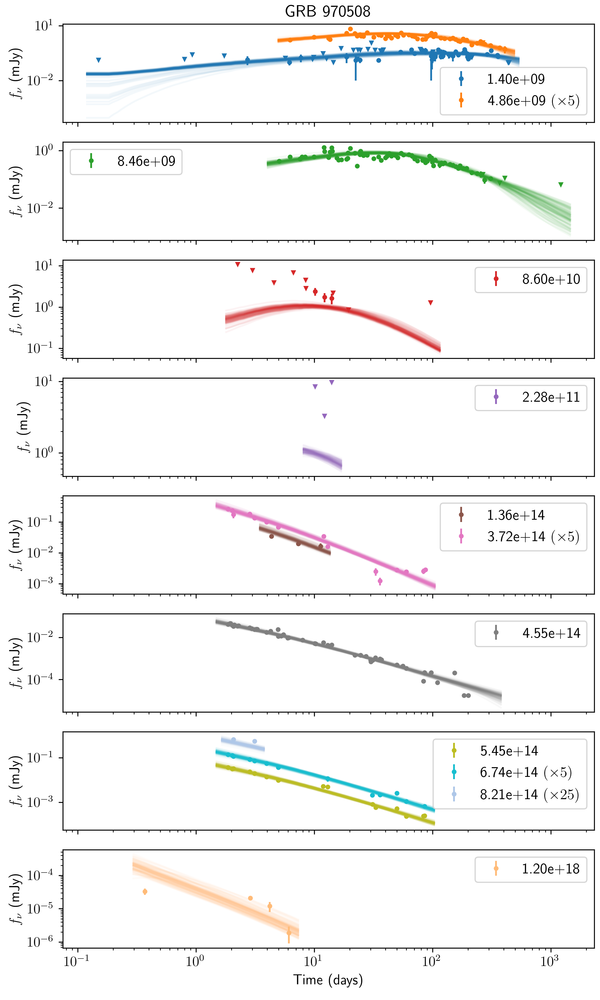
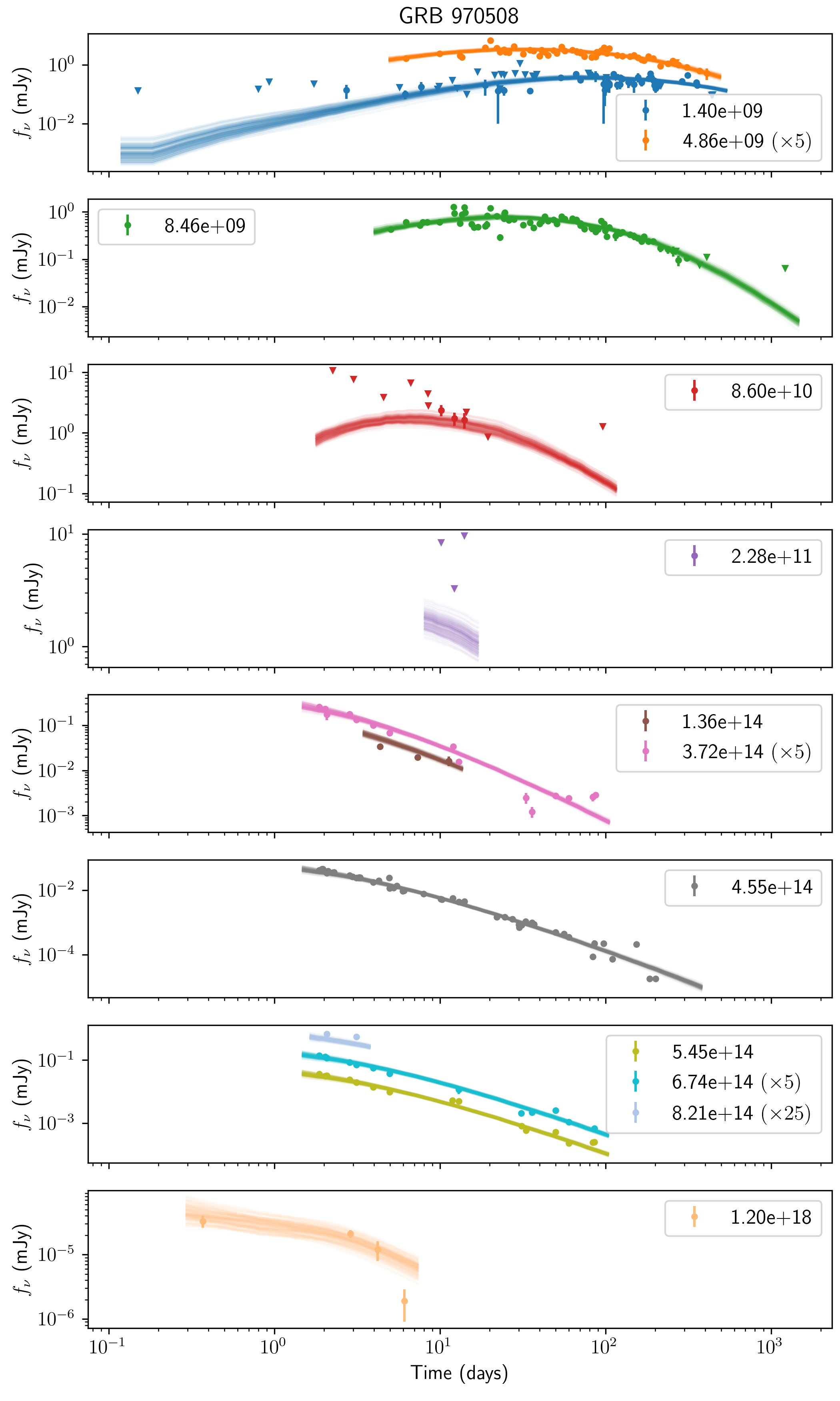
Figure 6: Fit results using DeepGlow for the dataset of GRB970508. The panels on the left side of the figure show the fit assuming an ISM progenitor environment while the panels on the right show the fit for a wind progenitor environment. The colored points correspond to the observed flux densities from the X-ray to radio bands. The legends of each subpanel display the observer frequency in Hz. The multiplication factor for a legend item indicates that the flux density is multiplied by this factor. The dots represent actual measurements while triangles correspond to the 3-$\sigma$ upper limits. From the posteriors of Fig. 4 and Fig. 5, respectively, 100 parameter sets are drawn randomly and the DeepGlow light curves are computed and shown as semi-transparent solid lines. More opaque regions thus correspond to higher posterior probabilities.

Table 3: Median values of the marginal posterior distributions for the afterglow parameters of GRB970508 assuming an ISM environment. Quoted uncertainties are at the 68% level. A match indicates if the uncertainty intervals overlap for the two afterglow models.

Parameter	DeepGlow	ScaleFit	Match
$\log_{10}\theta_{0}$	$0.02^{+0.13}_{-0.08}$	$-0.17^{+0.09}_{-0.09}$	$\quad\times$
$\log_{10}E_{K,\mathrm{iso}}$	$52.60^{+0.11}_{-0.15}$	$52.56^{+0.13}_{-0.12}$	$\quad\checkmark$
$\log_{10}n_{\mathrm{ref}}$	$0.66^{+0.33}_{-0.33}$	$-0.12^{+0.40}_{-0.39}$	$\quad\times$
$\theta_{\mathrm{obs}}/\theta_{0}$	$0.77^{+0.10}_{-0.12}$	$0.72^{+0.05}_{-0.05}$	$\quad\checkmark$
$p$	$2.51^{+0.04}_{-0.04}$	$2.39^{+0.06}_{-0.05}$	$\quad\times$
$\log_{10}\epsilon_{B}$	$-3.58^{+0.44}_{-0.39}$	$-2.64^{+0.58}_{-0.63}$	$\quad\checkmark$
$\log_{10}\bar{\epsilon}_{e}$	$-0.68^{+0.11}_{-0.11}$	$-0.94^{+0.14}_{-0.14}$	$\quad\times$
$A_{V}$	$0.08^{+0.03}_{-0.04}$	$0.05^{+0.03}_{-0.03}$	$\quad\checkmark$

Table 4: Same as Table 4, except now assuming a wind progenitor environment.

Parameter	DeepGlow	ScaleFit	Match
$\log_{10}\theta_{0}$	$0.09^{+0.07}_{-0.06}$	$0.06^{+0.02}_{-0.02}$	$\quad\checkmark$
$\log_{10}E_{K,\mathrm{iso}}$	$53.48^{+0.13}_{-0.14}$	$53.33^{+0.16}_{-0.20}$	$\quad\checkmark$
$\log_{10}n_{\mathrm{ref}}$	$2.72^{+0.18}_{-0.14}$	$2.33^{+0.21}_{-0.20}$	$\quad\times$
$\theta_{\mathrm{obs}}/\theta_{0}$	$1.13^{+0.04}_{-0.05}$	$1.10^{+0.03}_{-0.03}$	$\quad\checkmark$
$p$	$2.66^{+0.04}_{-0.04}$	$2.58^{+0.05}_{-0.05}$	$\quad\checkmark$
$\log_{10}\epsilon_{B}$	$-5.64^{+0.35}_{-0.38}$	$-4.73^{+0.48}_{-0.51}$	$\quad\times$
$\log_{10}\bar{\epsilon}_{e}$	$-0.21^{+0.12}_{-0.11}$	$-0.41^{+0.13}_{-0.11}$	$\quad\checkmark$
$A_{V}$	$0.04^{+0.02}_{-0.03}$	$0.07^{+0.03}_{-0.03}$	$\quad\checkmark$

We show the posteriors in Figure 4 (ISM environment) and Figure 5 (wind environment). The median values and 68% credible intervals of each parameter, and if these values overlap for DeepGlow and ScaleFit, are given in Table 4 (ISM environment) and Table 4 (wind environment). Note that the values presented here for ScaleFit are somewhat different than those in A22 because we have calculated, for simplicity, the median and not the mode of the distributions. Furthermore, small sampling differences between parameter estimation runs can arise as well.

For the most part, the parameter estimates of DeepGlow and ScaleFit overlap fairly well. For both environments, the estimates for $E_{\mathrm{K,iso}}$ and $\theta_{\mathrm{obs}}/\theta_{0}$ in particular are in good agreement between the two afterglow models. An exact match for all parameters is not expected in any case, as ScaleFit does have some distinct differences over BOXFIT, as mentioned. For the marginalized distributions that do not overlap within 1$\sigma$, there is usually only a slight discrepancy. Furthermore, strong correlations between parameters, e.g. $n_{\mathrm{ref}}$ and $\epsilon_{B}$, are captured well by DeepGlow in accordance with ScaleFit.

A big benefit of nested sampling is the direct computation of the Bayesian evidence $\mathcal{Z}$ as part of the sampling procedure. This allows us to give both a preference in terms of the progenitor environment as well as the afterglow model by calculating the ratio of evidence values, i.e. the Bayes factor $\mathrm{BF}$. We follow Kass & Raftery (1995) for interpretation.

We find a decisive preference for the wind environment over the ISM environment for both DeepGlow and ScaleFit with $\mathrm{BF}_{\mathrm{wind/ISM}}\sim 10^{4}$ and $\mathrm{BF}_{\mathrm{wind/ISM}}\sim 10^{3}$, respectively, similar to what was found in A22. We also find a strong preference for DeepGlow over ScaleFit in the ISM case with $\mathrm{BF}_{\mathrm{DG/SF}}\sim 20$ and a decisive preference in the wind case with $\mathrm{BF}_{\mathrm{DG/SF}}\sim 10^{3}$.

An important caveat to the parameter estimates of DeepGlow for the wind environment, is that for most values of $\bar{\epsilon}_{e}$ and $p$ in the posterior, $\epsilon_{e}$ becomes greater than one which is unphysical. To a lesser degree, this is true for the posterior of ScaleFit (wind environment) as well. In these instances, instead of setting $\xi_{N}=1$, a lower value is perhaps better suited, e.g. $\xi_{N}=0.1$, to scale down the other degenerate parameters ($E_{\mathrm{K,iso}}$, $n_{\mathrm{ref}}$, $\bar{\epsilon}_{e}$, and $\epsilon_{B}$) to more physical values (Eichler & Waxman, 2005). As in most literature, including A22 though not in Aksulu et al. (2020), $\xi_{N}$ is fixed canonically to 1, we did not use another value in our study here.

In Fig. 6, we plot the broadband GRB970508 dataset we fitted using DeepGlow. We drew 100 parameter sets randomly from the posteriors in Fig. 4 and Fig. 5 and drew the resulting light curve for each set using DeepGlow. This gives a visual confirmation that the fits are of good quality for both progenitor environments.

Overall, the results for DeepGlow and ScaleFit seem consistent. While additional systematics by DeepGlow compared to BOXFIT could change the results slightly, see the next section, we contend that a direct fit with BOXFIT would produce similar results to DeepGlow. Characterizing other GRB afterglow datasets with DeepGlow could thus provide an interesting avenue for a more thorough comparison between the physics of BOXFIT and ScaleFit.

4.3 Systematics

To characterize the systematics of DeepGlow, we reran the fit on GRB970508 assuming a wind environment. We used a different NN realisation this time from the same training run but trained for 1940 epochs. It has a very similar median error calculated over all data points in the test dataset compared to the primary NN realisation used which was trained for 1900 epochs, see A. Because the MaxFE on some reproduced light curves can become quite large, we may expect significant variation for some data points in the light curves generated between two NN realisations with slightly different weights. Any resulting change in the parameter estimates will give an indication on the influence of the systematic reproduction errors in DeepGlow. We show the results in Table 5.

The estimates are close and readily within the $1\sigma$ uncertainties for all parameters. Still, even though the overall error is much below the typical measurement error for both NN realisations, there are some variations in the estimated parameters. These are larger than any sampling differences we observed for DeepGlow runs. We attribute these variations to the large MaxFE for certain light curves. While this is not a substantial source of systematic errors, it is something to be taken into consideration.

Parameter	DeepGlow	Alt. NN	Match
$\log_{10}\theta_{0}$	$0.09^{+0.07}_{-0.06}$	$0.10^{+0.06}_{-0.05}$	$\quad\checkmark$
$\log_{10}E_{K,\mathrm{iso}}$	$53.48^{+0.13}_{-0.14}$	$53.46^{+0.11}_{-0.13}$	$\quad\checkmark$
$\log_{10}n_{\mathrm{ref}}$	$2.72^{+0.18}_{-0.14}$	$2.66^{+0.18}_{-0.15}$	$\quad\checkmark$
$\theta_{\mathrm{obs}}/\theta_{0}$	$1.13^{+0.04}_{-0.05}$	$1.11^{+0.04}_{-0.04}$	$\quad\checkmark$
$p$	$2.66^{+0.04}_{-0.04}$	$2.64^{+0.04}_{-0.04}$	$\quad\checkmark$
$\log_{10}\epsilon_{B}$	$-5.64^{+0.35}_{-0.38}$	$-5.46^{+0.35}_{-0.38}$	$\quad\checkmark$
$\log_{10}\bar{\epsilon}_{e}$	$-0.21^{+0.12}_{-0.11}$	$-0.28^{+0.12}_{-0.11}$	$\quad\checkmark$
$A_{V}$	$0.04^{+0.02}_{-0.03}$	$0.05^{+0.02}_{-0.03}$	$\quad\checkmark$

Table 5: Same as Table 4, except now comparing two realizations of DeepGlow from the same training run, see text.

5 DISCUSSION AND OUTLOOK

5.1 DeepGlow use cases

The current version of DeepGlow emulates the GRB afterglow simulations of BOXFIT with high accuracy. The data for the emulator was generated during $\sim$$10^{5}$ core hours and the emulator now produces individual light curves within a few milliseconds. This efficiency is best put to use for enabling population studies that require a large number of model runs (e.g., ¿10⁶ for Aksulu et al. 2022; $\sim$$10^{7}$ for Boersma & van Leeuwen 2022). There, DeepGlow speeds up iterations to run within of order an hour, offering astronomers an interactive exploration approach.

The quick turn-around time may also be beneficial in getting a first estimate of the underlying parameters from x-ray and optical detections of an afterglow, and inform the radio follow-up campaign. Before day 1 there is a $\sim$15% chance the BOXFIT-based training data was incomplete (Fig. 1). Our light curves with $\mathrm{MaxFE}>$10 lie mostly in this range. Only 1-4% of the pruned total have $\mathrm{MaxFE}>$10. Over day 1$-$10 both the validity of BOXFIT and the accuracy of DeepGlow improve considerably (Section 2.1). During real-life detections, estimates should thus be updated daily to benefit from the increased BOXFIT coverage during these first 10 days.

Application to afterglows may be especially relevant if the BOXFIT/DeepGlow top-hat jet is preferred for producing a reliable light curve shape and flux. One reason for this preference could be that the geometry of the transient indicates the jet travels in the direction of the observer, as is generally the case in GRBs. Even for potentially more off-axis systems such as gravitational-wave events, DeepGlow can be applicable and even preferred. In the intermediate phase of the afterglow, physical models (and hence, DeepGlow) outperform semi-analytic ones in the prediction of radio light-curve fluxes (Ryan et al., 2020). Furthermore, the top-hat jet core dominates the afterglow in these geometries too, once the light curve peaks (Gill et al., 2019; Duque et al., 2019).

In cases where a structured jet is required, the current version of DeepGlow is not the best choice.

5.2 Future outlook

The methods presented here could be extended to emulate more complex afterglow models. For GRBs, one example is GAMMA (Ayache et al., 2021). It incorporates a precise but highly computationally expensive local cooling approach to the evolution of micro-physical states. Current computational resources reasonably available would not suffice to run such models the roughly $10^{5}$ times required for accurate emulation using the methods in this work. Instead, a transfer learning approach using DeepGlow as the starting point could prove very valuable and greatly bring down the amount of repeated evaluations required.

While GRBs are generally observed at boresight, the multi-frequency afterglows of gravitational-wave events are generally observed at an angle from the center of the jet. In these cases, emulating a structured jet would be appropriate. These could be based on the numerical hydrodynamical simulations of relativistic jets with Gaussian profiles (Kumar & Granot, 2003; Urrutia et al., 2022).

5.3 Open source

In the current work, we have implemented an neural-net emulator for BOXFIT in DeepGlow, and demonstrated its accuracy. To facilitate the inclusion of other, more precise or more applicable RHD models, we have made DeepGlow open source, and we encourage contributions. We will provide the necessary compute time to train such new or improved emulators.

6 CONCLUSION

In this work we introduce DeepGlow, an open-source deep learning emulator for the GRB afterglow simulations of BOXFIT. It can generate light curves and spectra to within a few percent accuracy in just a fraction of the BOXFIT evaluation time. It enables rapid characterization of GRB afterglow data using the complex radiative transfer simulations in BOXFIT without the need for a supercomputer. It has support for either an ISM or stellar wind progenitor environment and can be extended to other environments as well.

We estimate the parameters of the broadband GRB afterglow dataset of GRB970508 as a first test of DeepGlow. We find consistent results with an analytical model calibrated to BOXFIT and, in accordance with recent results from the literature, find a decisive preference for a stellar wind progenitor environment around this GRB source.

We thank Mehmet Deniz Aksulu for the extensive discussions on gamma-ray burst physics and Gaussian processes. We thank Hendrik van Eerten for enlightening conversations on BOXFIT and Eliot Ayache for his suggestions which proved instrumental to our deep learning approach. We further thank Daniela Huppenkothen and Anna Watts for comments and suggestions.

This research was supported by the Dutch Research Council (NWO) through Vici research program ’ARGO’ with project number 639.043.815 and through CORTEX (NWA.1160.18.316), under the research programme NWA-ORC.

Appendix A Additional Neural Network Accuracy Figures

In Figure 7 we show the median fractional error for the ISM environment NN aggregated over all data points in all light curves in our test dataset as a function of training dataset size. Each NN realisation is trained for 200 epochs. The error follows an approximate log-linear slope. Thus, while the error improves quickly at first, it becomes increasingly harder to increase the accuracy of our NNs by adding more training data.

In Figure 8 we show the median fractional error over all data points as a function of the amount of epochs trained. The error decreases rapidly for the first 200 epochs after which it starts to level off to an asymptotic value. The wind environment NN has a much noisier error trajectory compared to the ISM environment NN. This is likely because of the increased amount of light curves with incomplete coverage in the wind environment dataset. Furthermore, the light curves in the wind dataset with incomplete coverage usually have more zero flux values as well.

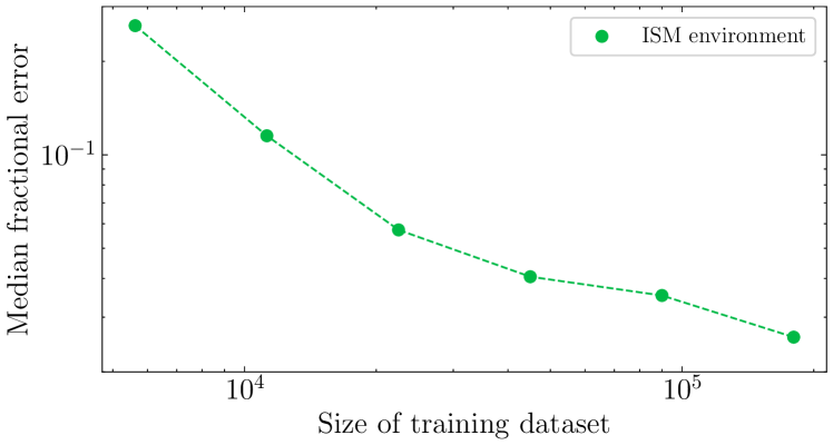
Figure 7: The median fractional error over the test dataset as a function of the training dataset size. The NN was trained for 200 epochs each time.

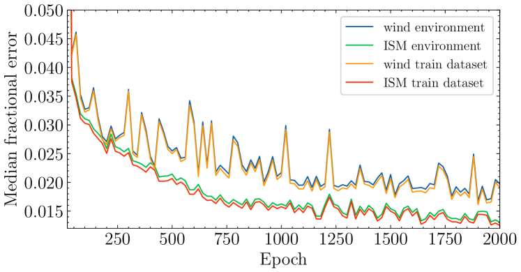
Figure 8: The median fractional error over the train and test dataset as a function of the amount of epochs trained. The ISM environment NN is shown in green (test dataset) or red (train dataset) while the wind environment NN is shown in blue (test dataset) or orange (train dataset).

References

- Abbott et al. (2017a) Abbott, B. P., Abbott, R., Abbott, T. D., et al. 2017a, The Astrophysical Journal, 848, L13
- Abbott et al. (2017b) Abbott, B. P., Abbott, R., Abbott, T. D., et al. 2017b, Physical Review Letters, 119, 161101
- Aksulu et al. (2020) Aksulu, M. D., Wijers, R. A. M. J., van Eerten, H. J., & van der Horst, A. J. 2020, Monthly Notices of the Royal Astronomical Society, 497, 4672
- Aksulu et al. (2022) Aksulu, M. D., Wijers, R. A. M. J., van Eerten, H. J., & van der Horst, A. J. 2022, Monthly Notices of the Royal Astronomical Society, 511, 2848
- Alexander et al. (2017) Alexander, K. D., Berger, E., Fong, W., et al. 2017, The Astrophysical Journal, 848, L21
- Ayache et al. (2021) Ayache, E. H., van Eerten, H. J., & Eardley, R. W. 2021, Monthly Notices of the Royal Astronomical Society, 510, 1315
- Blandford & McKee (1976) Blandford, R. D. & McKee, C. F. 1976, The Physics of Fluids, 19, 1130
- Boersma & van Leeuwen (2022) Boersma, O. M. & van Leeuwen, J. 2022, Astronomy & Astrophysics, 664, A160
- Boersma et al. (2021) Boersma, O. M., van Leeuwen, J., Adams, E. A. K., et al. 2021, Astronomy & Astrophysics, 650, A131
- Buchner et al. (2014) Buchner, J., Georgakakis, A., Nandra, K., et al. 2014, Astronomy & Astrophysics, 564, A125
- Caruana et al. (2000) Caruana, R., Lawrence, S., & Giles, L. 2000, in Proceedings of the 13th International Conference on Neural Information Processing Systems, NIPS’00 (Cambridge, MA, USA: MIT Press), 381
- Chornock et al. (2017) Chornock, R., Berger, E., Kasen, D., et al. 2017, The Astrophysical Journal, 848, L19
- Costa et al. (1997) Costa, E., Frontera, F., Heise, J., et al. 1997, Nature, 387, 783
- Coulter et al. (2017) Coulter, D. A., Foley, R. J., Kilpatrick, C. D., et al. 2017, Science, 358, 1556
- Cybenko (1989) Cybenko, G. 1989, Mathematics of Control, Signals and Systems, 2, 303
- Duque et al. (2019) Duque, R., Daigne, F., & Mochkovitch, R. 2019, Astronomy & Astrophysics, 631, A39
- Eichler & Waxman (2005) Eichler, D. & Waxman, E. 2005, The Astrophysical Journal, 627, 861
- Feroz et al. (2009) Feroz, F., Hobson, M. P., & Bridges, M. 2009, Monthly Notices of the Royal Astronomical Society, 398, 1601
- Gao et al. (2013) Gao, H., Lei, W.-H., Zou, Y.-C., Wu, X.-F., & Zhang, B. 2013, New Astronomy Reviews, 57, 141
- Gehrels et al. (2004) Gehrels, N., Chincarini, G., Giommi, P., et al. 2004, The Astrophysical Journal, 611, 1005
- Gill et al. (2019) Gill, R., Granot, J., De Colle, F., & Urrutia, G. 2019, The Astrophysical Journal, 883, 15
- Granot & Sari (2002) Granot, J. & Sari, R. 2002, The Astrophysical Journal, 568, 820
- Haggard et al. (2017) Haggard, D., Nynka, M., Ruan, J. J., et al. 2017, The Astrophysical Journal, 848, L25
- Hallinan et al. (2017) Hallinan, G., Corsi, A., Mooley, K. P., et al. 2017, Science, 358, 1579
- Higgins et al. (2019) Higgins, A. B., van der Horst, A. J., Starling, R. L. C., et al. 2019, Monthly Notices of the Royal Astronomical Society, 484, 5245
- Hornik et al. (1989) Hornik, K., Stinchcombe, M., & White, H. 1989, Neural Networks, 2, 359
- Kasim et al. (2021) Kasim, M. F., Watson-Parris, D., Deaconu, L., et al. 2021, Machine Learning: Science and Technology, 3, 015013
- Kass & Raftery (1995) Kass, R. E. & Raftery, A. E. 1995, Journal of the American Statistical Association, 90, 773
- Kerzendorf et al. (2021) Kerzendorf, W. E., Vogl, C., Buchner, J., et al. 2021, The Astrophysical Journal Letters, 910, L23
- Kumar & Granot (2003) Kumar, P. & Granot, J. 2003, The Astrophysical Journal, 591, 1075
- Leventis et al. (2012) Leventis, K., van Eerten, H. J., Meliani, Z., & Wijers, R. A. M. J. 2012, Monthly Notices of the Royal Astronomical Society, 427, 1329
- Nousek et al. (2006) Nousek, J. A., Kouveliotou, C., Grupe, D., et al. 2006, The Astrophysical Journal, 642, 389
- Panaitescu & Kumar (2002) Panaitescu, A. & Kumar, P. 2002, The Astrophysical Journal, 571, 779
- Pedregosa et al. (2011) Pedregosa, F., Varoquaux, G., Gramfort, A., et al. 2011, Journal of Machine Learning Research, 12, 2825
- Rasmussen & Williams (2006) Rasmussen, C. E. & Williams, C. K. I. 2006, Gaussian processes for machine learning, Adaptive computation and machine learning (Cambridge, Mass: MIT Press)
- Ryan et al. (2015) Ryan, G., Eerten, H. v., MacFadyen, A., & Zhang, B.-B. 2015, The Astrophysical Journal, 799, 3
- Ryan et al. (2020) Ryan, G., van Eerten, H., Piro, L., & Troja, E. 2020, The Astrophysical Journal, 896, 166
- Sari et al. (1998) Sari, R., Piran, T., & Narayan, R. 1998, The Astrophysical Journal, 497, L17
- Schmidhuber (2015) Schmidhuber, J. 2015, Neural Networks, 61, 85
- Schmit & Pritchard (2018) Schmit, C. J. & Pritchard, J. R. 2018, Monthly Notices of the Royal Astronomical Society, 475, 1213
- Smith (2015) Smith, L. N. 2015, arXiv e-prints, arXiv:1506.01186
- Sutskever et al. (2013) Sutskever, I., Martens, J., Dahl, G., & Hinton, G. 2013, in Proceedings of the 30th International Conference on Machine Learning (Pmlr), 1139
- Urrutia et al. (2022) Urrutia, G., De Colle, F., & López-Cámara, D. 2022, arXiv e-prints, arXiv:2207.07925
- Van Eerten et al. (2010) Van Eerten, H. J., Leventis, K., Meliani, Z., Wijers, R., & Keppens, R. 2010, Monthly Notices of the Royal Astronomical Society, 403, 300
- van Eerten et al. (2012) van Eerten, H. J., van der Horst, A., & MacFadyen, A. 2012, The Astrophysical Journal, 749, 44
- van Leeuwen et al. (2023) van Leeuwen, J., Kooistra, E., Oostrum, L., et al. 2023, Astronomy & Astrophysics, 672, A117
- Wijers et al. (1997) Wijers, R. A. M. J., Rees, M. J., & Mészáros, P. 1997, Monthly Notices of the Royal Astronomical Society, 288, L51
- Ying (2019) Ying, X. 2019, Journal of Physics: Conference Series, 1168, 022022
- Yost et al. (2003) Yost, S. A., Harrison, F. A., Sari, R., & Frail, D. A. 2003, The Astrophysical Journal, 597, 459