Quantum simulation of two-dimensional $\mathrm{U(1)}$ gauge theory in Rydberg atom arrays

Abstract

Simulating $\mathrm{U(1)}$ quantum gauge theories with spatial dimension greater than one is of great physical significance yet has not been achieved experimentally. Here we propose a simple realization of $\mathrm{U(1)}$ gauge theory on triangular lattice Rydberg atom arrays. Within experimentally accessible range, we find that the effective model well simulates various aspects of the $\mathrm{U(1)}$ gauge theory, such as emergence of topological sectors, incommensurability, and the deconfined Rokhsar-Kivelson point. Our proposal is easy to implement experimentally and exhibits pronounced quantum dynamics compared with previous proposals realizing $\mathrm{U(1)}$ and $\mathbb{Z}_{2}$ gauge theories.

Introduction. — Quantum simulations based on programmable Rydberg atom arrays have recently emerged as a powerful platform exploring exotic many-body physics of strongly correlated systems. Rydberg simulators allows for flexible design of lattice geometry with optical tweezers [1, 2], as well as wide tunability of interaction strength that goes far beyond conventional condensed matter experiments [3, 4]. A key element of quantum many-body simulations in Rydberg arrays is the Rydberg blockade mechanism, in which van der Waals interactions strongly suppress double occupancy of atomic Rydberg excitations within a certain blockade radius $R_{c}$ [5, 6, 7]. In particular systems, the Rydberg blockade can lead to low-energy local constraints that provide a natural implementation of lattice gauge theories [8, 9, 10, 11], a host of a large class of exotic quantum phenomena such as quantum spin liquids [12, 13, 14], fractionalized excitations with Abelian and non-Abelian statistics [15, 16]. Very recently, significant progress has been made realizing $\mathbb{Z}_{2}$ gauge theories in two spatial dimension with Rydberg platforms, in which $\mathbb{Z}_{2}$ topological order has been first observed [17]. Compared with $\mathbb{Z}_{2}$ gauge theories, $\mathrm{U(1)}$ gauge theories involve more exotic phenomena like sub-extensive topological sectors [18, 19], incommensurability[20, 21, 22], and deconfined quantum criticality [23, 21, 19, 24]. Nevertheless, the implementation of $\mathrm{U(1)}$ gauge theories involve complicated theoretical proposals [25], and have not been achieved in Rydberg experiments until recently.

One natural implementation of $\mathrm{U(1)}$ gauge theory is the dimer model on bipartite lattices [19, 26, 27, 28, 29, 30]. In particular, the dimer model on the honeycomb lattice is dual to the antiferromagnetic transverse field Ising model on triangular lattice [31, 22, 32], which can be easily implemented on Rydberg arrays with properly tuned detuning $\delta$ such that half filling of Rydberg atoms on average is achieved. In fact, the Rydberg arrays on triangular lattice has been studied in experiments [33] and numerical simulations [34] previously. Ordered states with $1/3$ and $2/3$ Rydberg fillings have been clearly identified. However, in between lies the ‘order-by-disorder’ (OBD) [35, 36, 37, 38, 39] region, in which physics remains unclear. This is exactly the region where the $\mathrm{U}(1)$ gauge theory is likely to sit.

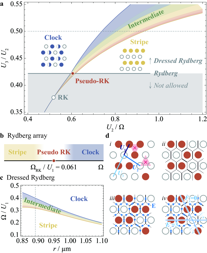
Figure 1: Phase diagram for the model Eq. (1) at half Rydberg filling with $\delta/U_{1}=3.188$. a, phase diagram on the $U_{3}/U_{2}$ plane; the dark gray line denotes the parameters that can be realized by Rydberg array; the white region denotes the parameter region realistic for dressed Rydberg array; the dashed grey line shows the parameter taken in Fig. 2. b, phase diagram of standard Rydberg atoms. c, phase diagram for the dressed Rydberg array; for the dressed state parameters are chosen as $\Omega/2\pi=10\ \mathrm{MHz}$, $\delta/2\pi=100\ \textrm{MHz}$ and $c_{6}=1000\ \mathrm{MHz\>\mu m^{6}}$; the dashed grey line shows the parameter taken in Fig. 2. d, Illustration of the emergent $\mathrm{U}(1)$ gauge structure; i, Illustration of the interactions and the ‘triangle-rule’ local constraint. Constraint-violating triangles are marked shaded with crossings; ii, Mapping of atom configurations to the fully-packed dimers; iii, charge-free gauge field; and iv, Illustration of emergent topological sectors.

In this Letter, we propose a simple realization of $\mathrm{U}(1)$ lattice gauge theories in Rydberg systems with atoms arranged on a triangular lattice array. Complement to previous studies, we focus on the half Rydberg filling case, and look into the detailed structures inside this OBD region. We analyze the effective model with large-scale quantum Monte Carlo simulations. Within experimental accessible range, we find that the effective model well simulates various aspects of $\mathrm{U(1)}$ gauge theory, including emergence of topological sectors and incommensurate phases, as well as the deconfined Rokhsar-Kivelson (RK) point. Our proposal is easy to implement and exhibits pronounced quantum dynamics compared with previous proposals realizing $\mathrm{U(1)}$ and $\mathbb{Z}_{2}$ gauge theories [25, 40].

Rydberg model on a triangular lattice. — We consider that neutral atoms are arranged into a triangular lattice array. As a minimum model, each atom can be regarded as a two-level system with $|g\rangle_{i}$ and $|r\rangle_{i}$, representing the ground state and the excited Rydberg state of the atom at site $i$, respectively. The Rydberg atom array is described by the following many-body Hamiltonian

$$H=\sum_{i}\left[-\frac{\Omega}{2}\left(|r\rangle_{i}\langle g|+|g\rangle_{j}\langle r|\right)-\delta|r\rangle_{i}\langle r|\right]\\ +\sum_{ij}U_{ij}|r\rangle_{i}\langle r|\otimes|r\rangle_{j}\langle r|,$$ (1)

where $\Omega$ is the Rabi frequency, $\delta$ is the detuning, and $U_{ij}$ is the interaction between the excited Rydberg states. In typical Rydberg systems, the Rydberg states are subjected to a long-range van der Waals interactions $U_{ij}\sim r_{ij}^{-6}$. However, for dressed Rydberg atoms the interaction is modified to a more complicated form where the decay is slower at short distance and the asymptotic behavior stays the same [41, 42].

The half filling condition of the Rydberg atoms can be tuned by $\delta$, which acts as the chemical potential of the Rydberg atoms. At $\delta=\frac{1}{2}\sum_{j\neq i}U_{ij}=3.188U_{1}$, where $U_{1}$ is the nearest neighbor interaction, the Hamiltonian exhibit an additional $\mathbb{Z}_{2}$-symmetry $\mathscr{P}$ which exchanges the Rydberg state and the ground state $\mathscr{P}|g\rangle_{i}=|e\rangle_{i}$, $\mathscr{P}|e\rangle_{i}=|g\rangle_{i}$. The Hamiltonian can be further mapped onto a spin-$1/2$ transverse field Ising model by identifying the Rydberg and ground state as spin-up and spin-down [4],

$$H=\sum_{ij}U_{ij}S_{i}^{z}S_{j}^{z}-\Omega\sum_{i}S_{i}^{x}.$$ (2)

As will be discussed later, this $\mathbb{Z}_{2}$ symmetry enables an extra mapping to the quantum dimer model and subsequently the emergence of $\mathrm{U}(1)$ gauge field and several interesting orders, which has been previously missed in the phase diagram.

Phase diagram. — We numerically investigate the model (1) with large scale quantum Monte-Carlo simulations [43, 44, 45, 41]. As the interaction is negligible at long distance, we truncate the interaction at the third-nearest-neighbor and study the phase diagram on the $U_{2}$-$U_{3}$ plane, where $U_{i}$ is the $i$-th-nearest-neighbor interaction. The simulations are performed on $L\times L$ lattices ($L=24,36$) with periodic boundary condition, and the temperature is set to $T=L^{-2}U_{1}$.

In the phase diagram we find various density wave orders. With small $U_{3}/U_{2}$, the two-sublattice stripe order is stabilized, while with large $U_{3}/U_{2}$ the three-sublattice clock order is stabilized. When $U_{2}$ and $U_{3}$ are small, the transition between the clock and the stripe phase is trivially first-order. As $U_{2}$ and $U_{3}$ exceeds some critical value, a fan of intermediate states emerge at the clock-to-stripe boundary. The intermediate region is separated with the clock phase through a first-order phase transition and with the stripe phase through a continuous one. The clock-stripe transition line and the fan-shaped region terminate at a single multicritical point. The position of the multicritical point is determined by the intersection between the clock-to-stripe and the stripe-to-intermediate transition lines. Through a finite size scaling analysis, we extrapolate its position in thermodynamic limit to be $U_{2c}/\Omega=0.547(5)$ and $U_{3c}/\Omega=0.215(3)$.

Emergent $\mathrm{U(1)}$ gauge field and topological sectors. — The structure of the phase diagram resembles that of the quantum dimer model on the honeycomb lattice, which is dual to a $\mathrm{U(1)}$ lattice gauge theory. To better understand the phase diagram, we start with the limit where $U_{1}$ becomes the dominant energy scale $U_{1}\gg|\Omega|,|U_{2}|,|U_{3}|$. At half Rydberg filling, the Hamiltonian can be recast in the following form

$$H_{U_{1}}=\frac{U_{1}}{2}\sum_{\triangle}\left(\sum_{i\in\triangle}|r\rangle_{i}\langle r|-\frac{3}{2}\right)^{2}+\mathrm{const}.$$ (3)

It is clear that the ground state must satisfy a local constraint that either one or two occupations of Rydberg states are allowed within each unit triangle, while zero or three occupations are not allowed, see Fig. 1di. The freedom of Rydberg filling within each unit triangle is guaranteed by half Rydberg filling, which give rise to the extensive ground state degeneracy. The local filling constraint within each triangle serves as the key ingredient of the emergent $\mathrm{U(1)}$ gauge field: we define the emergent electric field on the (oriented) link of the dual honeycomb lattice. The value of the electric field (from A to B sublattice) is assigned 2 if the triangular lattice bond crossing this link is frustrated, and is assigned -1 otherwise. Here we define a bond is ‘frustrated’ if the two sites connected to this bond is occupied by the atomic states with the same type (both $|g\rangle$ or both $|r\rangle$). Notice that the above local constraint dictates that each unit triangle consists one and only one frustrated bond, which translates to the charge-free condition of the $\mathrm{U(1)}$ gauge field at each dual vertex $\mathbf{v}$ (see Fig. 1diii):

$$Q_{\mathbf{v}}\equiv(\textrm{div}E)_{\mathbf{v}}=0.$$ (4)

Also notice that this electric field configuration on the dual honeycomb lattice is equivalent to the fully packed dimer coverings: by assigning each $E=2$ link with one dimer and the $E=-1$ link with no dimer, each vertex will be covered by exactly one dimer, see Fig. 1div.

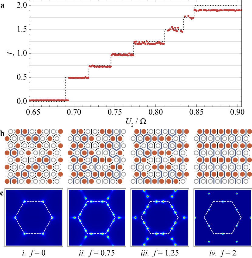
Figure 2: Properties of the intermediate phase. a, Flux density $f$ as a function of $U_{2}/\Omega$. b,c, Real space patterns (b) and structural factor of Rydberg density (c) at different topological sectors. The data are simulated along the line $U_{2}=2U_{3}$ (Fig. 1a and c) at system size $L=24$ and inverse temperature $\beta=L^{2}$.

A direct consequence of the $\mathrm{U(1)}$ gauge structure is the emergence of topological sectors, which can be defined as follows [28]. For the two cuts $\mathscr{C}_{x}$ and $\mathscr{C}_{y}$ throughout the lattice (illustrated in Fig. 1div), the corresponding electric fluxes that penetrates through the cuts are conserved quantities upon local fluctuations. Therefore, the low-energy Hilbert space can be divided into different topological sectors labeled by such fluxes $(F_{x},F_{y})$. For the ground states, one of the fluxes is zero. Without losing of generality, we set $F_{y}=0$ and use the flux density $f\equiv F_{x}/L_{x}$ to label topological sectors.

The emergent $\mathrm{U(1)}$ gauge structure in the large $U_{1}$ limit is robust against local perturbations such as $U_{2}$, $U_{3}$ and $\Omega$. As illustrated in Fig. 1a, various density orders at different topological sectors are stabilized as the ground states in the phase diagram. These density wave orders can be also characterized by the ordering wave vectors in the Rydberg structural factor:

$$\mathcal{S}(\textbf{Q})=\frac{1}{N}\sum_{ij}\langle(n_{i}-\frac{1}{2})(n_{j}-\frac{1}{2})\rangle e^{i\textbf{Q}\cdot(\textbf{r}_{i}-\textbf{r}_{j})},$$ (5)

where $n_{i}=|r\rangle_{i}\langle r|$ is the occupancy of the Rydberg atom at site $i$.

The flux densities $f$, real-space configurations and the Rydberg structural factors of each density orders are illustrated in Fig. 2. The three-sublattice ‘clock’ state has the ordering wave vector at the K point, and lives within the $f=0$ topological sector. The ‘clock’ state is named after the six-fold clock anisotropy of the order parameter, as clearly illustrated in the order parameter histogram in Fig. 3bi. This clock anisotropy arise from the OBD mechanism, by which quantum fluctuations allow tunneling within the macroscopically degenerate manifold, pick up the three-sublattice order, and open a gap to the excitations [35, 36, 37, 38, 39].

The two-sublattice ‘stripe’ state is ordered at the M point with saturated flux density $f=2$. In between the ‘clock’ and the ‘stripe’ state lives a fan of intermediate phases with $0<f<2$. The ordering wave vector Q is typically incommensurate between the K and the M point, and is related with $f$ by $\mathbf{Q}=\left(\pm\frac{2(1-2f)\pi}{3},\pm\frac{2\pi}{\sqrt{3}}\right)$ and symmetry equivalent wave vectors.

Multicritical RK point as $(2+2)$d QED. — The most interesting aspect of our model is the correspondence of the multicritical point to the RK point of the quantum dimer model (QDM) [46, 19], by comparing the overall phase diagram with the generic QDM on the honeycomb lattice [21, 28]. RK point is a quantum critical point separating clock and stripe states, and supports deconfined charge excitations right at the critical point [27, 19]. It is described by a free Gaussian theory that supports quadratically dispersive gapless photons [47, 48]. On the honeycomb lattice, RK point is multicritical with two relevant perturbations [20, 21, 28], hence can be achieved by tuning two system parameters. In the following, we present a series of numerical evidence to prove that the multicritical point indeed corresponds to the RK point.

A characteristic feature of the RK point is that the ground states within different topological sectors are exactly degenerate [47, 19]. To verify this feature, we measure the ground state energies within different topological sectors at the multicritical point with $L=24$. We find vanishing energy differences between different topological sectors $\sim 6\times 10^{-4}L^{2}\Delta$. The tiny difference may be accounted by the marginally and dangerously irrelevant terms [20, 21], which do not vanish at finite system size. This proximate degeneracy strongly indicates that the multicritical point corresponds to the RK point.

Further evidence of RK point is examined by the correlation behaviors at the multicritical point. We first measure the electric field correlator $C_{E}(\vec{\mathsf{R}}-\vec{\mathsf{R}}^{\prime})=\langle\psi_{E}^{*}(\vec{\mathsf{R}})\psi_{E}^{\phantom{*}}(\vec{\mathsf{R}}^{\prime})\rangle$, where

$$\psi_{E}=E_{\textbf{b}_{1}}+E_{\textbf{b}_{2}}\mathrm{e}^{-\mathrm{i}2\pi/3}+E_{\textbf{b}_{3}}\mathrm{e}^{\mathrm{i}2\pi/3}$$ (6)

is the order parameter of the electric field. Here $E_{\textbf{b}_{i}}$, $i=1,2,3$ represents the electric field along three direction as depicted in Fig. 1d. At RK point, the electric field correlator is predicted to follow the long distance behavior $C_{E}(\vec{\mathsf{R}})\sim|\vec{\mathsf{R}}|^{-2}$, following from the conservation of electric charges [41, 49]. Such behavior is clearly observed in our simulations (Fig. 3a, red line). We have also measured the Rydberg density correlator $C_{R}(\vec{\mathsf{R}}-\vec{\mathsf{R}}^{\prime})=\langle\psi_{R}^{*}(\vec{\mathsf{R}})\psi_{R}^{\phantom{*}}(\vec{\mathsf{R}}^{\prime})\rangle$, where

$$\psi_{R}=n_{A}+n_{B}\mathrm{e}^{\mathrm{i}2\pi/3}+n_{C}\mathrm{e}^{-\mathrm{i}2\pi/3}$$ (7)

is the order parameter of the clock density wave. The Rydberg correlator at RK point is predicted to satisfy the asymptotic form $C_{R}(\vec{\mathsf{R}})\sim|\vec{\mathsf{R}}|^{-1/2}$, also consistent with our numerical results (Fig. 3a, blue line).

Figure 3: a, Electric field and Rydberg density correlators $C_{E}(r)$ and $C_{R}(r)$ at the multicritical point. Our numerical results well agree with the theoretical predictions $C_{E}\sim r^{-2}$ and $C_{R}\sim r^{-1/2}$ indicated by dashed lines, respectively. The data are simulated at system size $L=36$ and inverse temperature $\beta=L^{2}$. b, Histogram of the clock order parameter $\psi_{R}$ measured in the clock phase (i), at the multicritical point (ii) and in the stripe phase (iii). The data are simulated at system size $L=24$ and inverse temperature $\beta=L^{2}$.

A hallmark of deconfined $\mathrm{U(1)}$ gauge theories is the presence of emergent continuous symmetries, which can be examined in the histogram of the order parameter. Here we examine the histograms of the clock order parameter around the multicritical point, see Fig. 3b. In the clock phase, the order parameter $\psi_{R}$ is pinned to six distinct values in the histogram, indicating relevance of instantons [50, 47, 20] (Fig. 3bi). For the stripe phase the histogram is shrunk into a central peak (Fig. 3biii) indicating absence of the three-sublattice ordering. At the multicritical point, we find that the $\mathrm{U(1)}$ symmetry emerges as a symmetric ring in the histogram (Fig. 3bii). The right presence of the emergent $\mathrm{U(1)}$ symmetry at the multicritical point is fully consistent with the scenario of the deconfined quantum critical point [23, 21, 19].

Excitations at the multicritical point.—Here we turn to the dynamical properties at the multicritical point. We measure the dynamical electric field and Rydberg density correlators:

$$G_{E}(\mathbf{q},\tau) =\frac{1}{L^{2}}\sum_{\mathbf{R,R^{\prime}}}e^{i(\mathbf{R}-\mathbf{R^{\prime}})\cdot\mathbf{q}}\langle E_{\mathbf{R}}^{y}(\tau)E_{\mathbf{R^{\prime}}}^{y}(0)\rangle,$$ (8)

$$G_{R}(\mathbf{q},\tau) =\frac{1}{L^{2}}\sum_{ij}e^{i(\mathbf{r}_{i}-\mathbf{r}_{j})\cdot\mathbf{q}}\langle n_{i}(\tau)n_{j}(0)\rangle.$$

Here $E_{\mathbf{R}}^{y}$ represent the electric field that origins from the site R along the $y$-direction. As for comparison, we have also measured the excitation spectra for the RK point of the RK-QDM using the diffusion Monte Carlo technique [51, 52, 41]. The spectra are obtained from the imaginary time correlations via the stochastic analytical continuation technique [53, 54, 55, 41]. As has been widely discussed in the context of QDM, at RK point two gapless quadratic excitations present in the electric field spectra [56, 57]: the ‘resonon’ around $\Gamma$ point that corresponds to the gauge photon excitations, and the ‘pi0n’ around $\mathrm{K}$ point due to the proximity to the three-sublattice ordered phase. These two quadratic excitations are indeed observed in our numerical spectra (Fig. 4a, c), consistent with the dynamical exponent $z=2$ at RK point. Further, the distinct curvatures of these two excitations [41] excludes band folding and indicates the distinct physical nature of these excitations.

As for the Rydberg density correlators, we observe only one branch of quadratic excitation stemming from the $\mathrm{K}$ point, with different curvatures from the previous resonon and pi0n. In fact, this excitation can be regarded as a fractionalized version of ‘pi0n’ that transform non-trivially under the symmetry group $\mathscr{P}$. Here we dub this new fractionalized excitation as ‘pi0n*’.

Figure 4: The excitation spectrum of the multicritical point. Electric field (a,c) and Rydberg density (b,d) dynamical correlation spectra of the Rydberg model Eq. (1) at the multicritical point (a,b) and the RK-QDM [46] at the RK point $v=t=1$ (c,d). The data are simulated at system size $L=24$, topological sector $f=0$ and inverse temperature $\beta=L^{2}$.

Advantages of our proposal. — Our proposal has several advantages compared with previous ones realizing two-dimensional gauge theories. In our proposal, only one species of atom is required and the arrangement is the simple triangular lattice. Moreover, our system exhibits significant low-energy quantum dynamics, as indicated by the pronounced bandwidth of the gauge excitations in Fig. 4. This phenomenon is quite unusual, as in general, the low-energy quantum dynamics of the gauge theories take the ring-exchange form, which often arise as a high-order perturbation in realistic systems [58, 59, 25, 17, 9, 10]. In our system, however, the ring-exchange process arises at the first order of the quantum fluctuation $\Omega$, owing to the peculiar mapping of our atomic model to the emergent gauge field. Hence the gauge fluctuation is relatively large at low energies. We believe that our system provides an ideal platform exploring exotic quantum aspects of gauge theories.

Discussions. — Simulating lattice gauge theories with spatial dimension greater than one is of intense interest and great physical significance. Our proposal of triangular lattice Rydberg atom array at half filling provide a simple and direct realization of the $\mathrm{U(1)}$ gauge theory in two spatial dimension. It also allows to investigate broad aspects of $\mathrm{U(1)}$ gauge theory physics such as emergent topological sectors, incommensuratibility and the RK point. Moreover, it provides an ideal platform to investigate topological excitations such as ‘spinons’ and ‘topological strings’ [60, 31, 22]. With rapid developments of the Rydberg platforms in the recent years, various measurements such as snapshots and non-local correlations now becomes possible that goes far beyond traditional condensed matter probes.

It is worth noting that the most interesting regime in the phase diagram locates at the boundary between the clock and stripe states, which turns out to be mostly accessible in standard Rydberg and dressed Rydberg experiments. For the standard Rydberg platform, the experimentally accessible regime is marked as the black thick line in Fig. 1, which cuts through the intermediate regime with negligible thickness. As the thickness of the intermediate regime is roughly proportional the magnitude of the relevant cubic anisotropy term near the RK point [21], it indicates that that one of the relevant perturbation is sufficiently small so that this intermediate regime lies sufficiently close to the celebrated RK point. Indeed it is supported by our numerical data [41]. Hence we claim that the RK point can be simulated directly with standard Rydberg experiments. With dressed Rydberg atoms [42, 41] one can access an extended regime of the phase diagram (marked as the unshaded region in Fig. 1) that includes the intermediate phases. This regime also host interesting physics, such as incommensurability, different topological sectors, and is even associated with potential deconfinement of gauge field [20, 21]. We expect to unveil the interesting physics of this regime with dressed Rydberg atom arrays.

Acknowledgments. — We wish to thank Rong Yu, Hai-Zhou Lu, Yuan Wan, Yin-Chen He, Yue Yu, Yiming Wang, Jiucai Wang and Chun-Jiong Huang for valuable discussions. C.L. thanks Rong Yu for hospitality inviting him to visit Renmin University of China where part of the work is done. This work is supported by the National Key Research and Development Program of China (Grants Nos. 2022YFA1403700, 2017YFA0304204, 2016YFA0300501 and 2016YFA0300504), the National Natural Science Foundation of China (Grants Nos. 11625416, 11474064, 11534001 and 11925402), and the Shanghai Municipal Government (Grants Nos. 19XD1400700 and 19JC1412702). X.-F.Z. acknowledges funding from the National Science Foundation of China under Grants No. 11804034, No. 11874094 and No.12047564, Fundamental Research Funds for the Central Universities Grant No. 2020CDJQY-Z003. Z.Y. thanks the supports of the seed fund for new staff of HKU (2201100367) and the open fund of the State Key Laboratory of Surface Physics , FDU (KF2021_13). C.L. is supported by the National Basic Research Program of China (2015CB921102), the Strategic Priority Research Program of the Chinese Academy of Sciences (XDB28000000), Guangdong province (2016ZT06D348, 2020KCXTD001), and the Science, Technology and Innovation Commission of Shenzhen Municipality (ZDSYS20170303165926217, JCYJ20170412152620376, KYTDPT20181011104202253).

Quantum simulation of two-dimensional $\mathrm{U(1)}$ gauge theory in Rydberg atom arrays

Supplemental Materials

1 Height field representation

In this section, we give an introduction to the height field representation of the two-dimensional U(1) gauge theories in the context of bipartite dimer model. The height representation was initially introduced in the context of triangular lattice frustrated Ising model [61], and it also applies for the dimer models via the spin-to-dimer mapping.

In the height representation, each hexagonal plaquette is assigned an integer number $\tilde{h}(\mathbf{r})$. Turning clockwise around a site of the even, the height $\tilde{h}(\mathbf{r})$ changes by $+1$ when crossing an empty link (or unfrustrated bond), and by $-2$ when crossing an occupied link (or frustrated bond).

Figure S1: An illustration of the height field. The red and blue points denote two sublattices on the dual lattice. The numbers in the center of hexagonal plaquettes illustrate the height field of the corresponding dimer configuration. The dark blue arrows denote the three unit vectors defined on the triangular lattice and its dual honeycomb lattice of dimers. The light orange and green paths denote the loop along which the winding numbers $F_{x}$ and $F_{y}$ are defined.

2 Effective field theory near the RK point

The most interesting physics of the QDM lies around the RK point. Here the RK point serve as a quantum critical point separating the clock and stripe ordered phases. The effective field theory in the vicinity of the RK point takes the form [47, 48, 61]

$$\mathscr{L}_{0}=\frac{1}{2}\left[(\partial_{\tau}h)^{2}+\kappa^{2}(\nabla^{2}h)^{2}\right]+\frac{\rho_{2}}{2}(\nabla h)^{2}+\lambda\cos 2\pi h,$$ (S1)

where $\rho_{2}\propto 1-v/t$ controls the phase transition, and $\lambda$ is the instanton term dictating the discrete nature of the height. When $\rho_{2}>0$, the instanton term $\lambda$ is relevant so that the system is pinned to the six-fold clock state; When $\rho_{2}<0$, the fluctuations of $\nabla h$ immediately become unbounded and saturates to its UV limit, where we obtain the staggered stripe state. The instanton term $\lambda$ becomes dangerously irrelevant at the critical point $\rho_{2}=0$, which corresponds to the RK point. The effective theory at RK point takes the form of the quantum Lifshitz model

$$\mathscr{L}_{\mathrm{QLM}}=\frac{1}{2}\left[(\partial_{\tau}h)^{2}+\kappa^{2}(\nabla^{2}h)^{2}\right]$$ (S2)

with dynamical exponent $z=2$. The fluctuating gauge field mediate short-range interactions between test charges, free from the confinement issue of pure $(2+1)\mathrm{d}$ $U$(1) gauge theories [50].

More recently, the fate of RK point under generic perturbations was discussed in refs. [20, 21]. On the honeycomb lattice, RK point also admit a relevant trigonal anisotropy $\mathscr{L}_{1}=g_{3}\prod_{\alpha=1}^{3}\left(\nabla h\cdot\hat{\mathbf{e}}_{\alpha}\right)$ in addition to a marginally irrelevant quartic coupling $\mathscr{L}_{2}=g_{4}\left(\nabla h\cdot\nabla h\right)^{2}$. Here $\hat{\mathbf{e}}_{\alpha}$ ($\alpha=1,2,3$) are the unit vectors aligned perpendicular to three dimer directions. Considering the whole theory

$$\mathscr{L}=\mathscr{L}_{0}+\mathscr{L}_{1}+\mathscr{L}_{2},$$ (S3)

it is shown that a sequence of commensurate and incommensurate regime with finite and non-saturated $f$ is stabilized in the vicinity of the RK point. This intermediate regime forms an incomplete ‘devil’s staircase’ structure, with the analogue to the fractal ‘Cantor set’ in mathematics. The incommensurate states host gapless phason mode that corresponds to the $U$(1) gauge photons, hence prevents gauge charges from confining. This scenario is dubbed as ‘Cantor deconfinement’ as is proposed in the seminal work [20].

3 Finite size scaling of the multicritical point

The phase diagram in the main text is simulated with system size $L=24$. To determine the location of multicritical point in the thermodynamic limit, we carried out a finite size scaling. The position of multicritical point is determined by the intersection of clock-stripe transition line and the stripe-intermediate transition line, i.e. $E(f=0)=E(f=2)=E(f=2-3/L_{x})$. Through an extrapolation, we determine the position of the multicritical point in the thermodynamic limit, which is $J_{2}=0.1093(11)$, $J_{3}=0.0429(7)$ (Fig. S2).

Figure S2: The finite size scaling which gives the position of the multicritical point in the thermodynamic limit.

4 Correlations at the multicritical point

We calculate the Rydberg density correlation at the multicritical point (Fig. S3). As for comparison, we measure the same correlator for the RK wavefunction of the RK-QDM. We restrict our update in Monte Carlo simulation to the topological sector $f=0$. We find that these two correlation functions agrees considerably well, which suggests the RK property of the multicritical point.

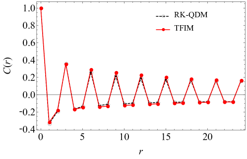
Figure S3: The spin-spin correlation function along $x$-axis, measured for the Rydberg model at the multicritical point (solid red) and the RK-QDM at the RK point (dashed black).

Here we evaluate the long-distance behaviors of order parameter correlators $C_{E}$ and $C_{R}$ at RK point. The asymptotic behaviors of correlators can be directly evaluated from field theory. Here we present a more intuitive way to understand the long-distance behaviors. The RK wave function of the RK-QDM is the equal-weight superposition of fully-packed dimer coverings $|\psi_{\mathrm{RK}}\rangle\sim\sum_{c}|c\rangle$. The observable $\hat{\mathscr{O}}$ with respect to this wave function $\langle\psi_{\mathrm{RK}}|\hat{\mathscr{O}}|\psi_{\mathrm{RK}}\rangle$ is equivalent to the statistical problem in classical dimer model at infinite temperature $T=\infty$, where the statistical weight of all dimer coverings are identical.

For the electric field correlator $C_{E}$, such statistical problem has already been solved in the context of dimer models [62]. The asymptotic behavior of the electric field correlator is predicted to be $C_{E}(\mathbf{R})\sim|\mathbf{R}|^{-2}$. For the Rydberg density correlator $C_{R}$, such statistical problem have been investigated in the context of classical antiferromagnetic Ising model on the triangular lattice [49], and the asymptotic behavior is predicted to be $C_{R}(\mathbf{r}_{i}-\mathbf{r}_{j})\sim|\mathbf{r}_{i}-\mathbf{r}_{j}|^{-1/2}$.

5 Linear-quadratic crossover

When far away from the multicritical point, two linear excitations are found at $\Gamma$ and $K$. When approaching the multicritical point, the dynamical exponent $z$ changes from $z=1$ to $z=2$. In the linear-quadratic crossover process (Fig. S4), the linear mode at $K$ softens into a quadratic mode, whereas the mode at $\Gamma$ gradually vanishes.

Figure S4: The linear-quadratic crossover in spin spectrum, measured at $J_{2}=0.05$ (a), $J_{2}=0.08$ (b), $J_{2}=0.1035$ (c) (multicritical point) and $J_{3}=0.0391$. $L=24$, $\beta=L^{2}/2=288$ is taken.

6 Curvatures of quadratic dispersions

To compare different excitations at the multicritical point, we extract dispersions of three quadratic excitations and fit them to the form

$$\omega=\frac{1}{2}C_{2}(\mathbf{q}-\mathbf{q}_{0})^{2}$$ (S4)

in vicinity of the gapless momenta $\mathbf{q}_{0}$. The results are shown in Table SI. We find the curvature of the pi0n* excitation in Rydberg density spectrum roughly twice the curvature of pi0n in electric field spectrum.

Table SI: The curvature defined in Eq. (S4) for different excitations measured in the Rydberg model and RK-QDM.

Excitations		Curvature $C_{2}$
		Rydberg model	RK-QDM
(Electric field)	resonon	$0.080(3)$	$0.61(3)$
	pi0n	$0.057(4)$	$0.36(4)$
(Rydberg density)	pi0n*	$0.095(2)$	$0.78(8)$

7 The intermediate regime

In the phase diagram, we find an interesting fan-shaped regime with intermediate ‘tilt’ $f$ at the clock-to-stripe boundary. Depending on the value of $f$, the spin structural factor is peaked at some intermediate wave vectors between the K and M points. The most exciting feature of this intermediate regime is that it meets the microscopic ingredients for the long sought ‘Cantor deconfinement’ scenario [20]. Due to the limited system size in our measurement, we are unable to observe the fractal structure of this regime. A detailed analysis of this regime is beyond the scope of this work. However, we notice a numerical work on a similar model with similar phase diagram [28], where the nature of the intermediate regime and its properties have been elaborately discussed in that work [28].

8 Stochastic series expansion (SSE)

For the numerical works in this paper, we use a QMC method with stochastic series expansion (SSE) algorithm [43, 44, 45] to simulate the ground state properties and imaginary time Green function. This method will be briefly introduced below. For convenience, in the simulation we work with the spin basis that has been introduced in the main text and is equivalent to the Rydberg occupation basis.

In quantum statistics, the measurement of observables is closely related to the calculation of partition function $Z$

$$\langle\mathscr{O}\rangle=\mathrm{tr}\>\left(\mathscr{O}\exp(-\beta H)\right)/Z,\quad Z=\mathrm{tr}\exp(-\beta H)$$ (S5)

where $\beta=1/T$ is the inverse temperature, $H$ is the Hamiltonian of the system and $\mathscr{O}$ is an arbitrary observable. Typically, in order to evaluate the ground state property, one takes a sufficiently large $\beta$ such that $\beta\sim L^{z}$, where $L$ is the system scale and $z$ is the dynamical exponent. In SSE, such evaluation of $Z$ is done by a Taylor expansion of the exponential and the trace is taken by summing over a complete set of suitably-chosen basis.

$$Z=\sum_{\alpha}\sum_{n=0}^{\infty}\frac{\beta^{n}}{n!}\langle\alpha|(-H)^{n}|\alpha\rangle$$ (S6)

We then write the Hamiltonian as the sum of a set of operators whose matrix elements are easy to calculate.

$$H=-\sum_{i}H_{i}$$ (S7)

In practice we truncate the Taylor expansion at a sufficiently large cutoff $M$ and it is convenient to fix the sequence length by introducing in identity operator $H_{0}=1$ to fill in all the empty positions despite it is not part of the Hamiltonian.

$$(-H)^{n}=\sum_{\{i_{p}\}}\prod_{p=1}^{n}H_{i_{p}}=\sum_{\{i_{p}\}}\frac{(M-n)!n!}{M!}\prod_{p=1}^{n}H_{i_{p}}$$ (S8)

and

$$Z=\sum_{\alpha}\sum_{\{i_{p}\}}\beta^{n}\frac{(M-n)!}{M!}\langle\alpha|\prod_{p=1}^{n}H_{i_{p}}|\alpha\rangle$$ (S9)

To the carry out the summation, a Monte Carlo procedure can be used to sample the operator sequence $\{i_{p}\}$ and the trial state $\alpha$ with according to their relative weight

$$W(\alpha,\{i_{p}\})=\beta^{n}\frac{(M-n)!}{M!}\langle\alpha|\prod_{p=1}^{n}H_{i_{p}}|\alpha\rangle$$ (S10)

For sampling we adopt a Metropolis algorithm where the configuration of one step is generated based on updating the configuration of the former step and the update is accepted at a probability

$$P(\alpha,\{i_{p}\}\rightarrow\alpha^{\prime},\{i^{\prime}_{p}\})=\min\left(1,\frac{W(\alpha^{\prime},\{i^{\prime}_{p}\})}{W(\alpha,\{i_{p}\})}\right)$$ (S11)

Diagonal update, where diagonal operators are inserted into and removed from the operator sequence, and cluster update, where diagonal and off-diagonal operates convert into each other, are adopted in update strategy.

In TFIM $H=J\sum_{b}S_{i_{b}}^{z}S_{j_{b}}^{z}-h\sum_{i}\sigma_{i}^{x}$, we write the Hamiltonian as the sum of following operators

$$H_{0} =1$$ (S12)

$$H_{i} =h(S_{i}^{+}+S_{i}^{-})/2$$

$$H_{i+n} =h/2$$

$$H_{b+2n} =J(1/4-S_{i_{b}}^{z}S_{j_{b}}^{z})$$

where a constant is added into the Hamiltonian for convenience. For the non-local update, a branching cluster update strategy is constructed [44], where a cluster is formed in $(D+1)$-dimensional by grouping spins and operators together. Each cluster terminates on site operators and includes bond operators (Fig. S5a). All the spins in each cluster is flipped together at a probability $1/2$ after all clusters are identified.

During the simulation process, a number of Monte Carlo steps, denoted $N_{t}$ are first used for thermalization, i.e., to let the system reach equilibrium. Then, $N_{m}$ steps are used for measurement. These steps are divided into $N_{b}$ bins, each containing $N_{0}=N_{m}/N_{b}$ steps. For some given observable $\mathscr{O}$, we first calculate its mean value within each bin $\bar{\mathscr{O}}_{b}=\frac{1}{N_{0}}\sum_{i=1}^{N_{0}}\mathscr{O}_{i}$, where $b=1,\cdots,N_{b}$ denotes the numbering of the bin and $i$ denotes the numbering of step within the bin. Then the expected value and the error bar of the observable are given by

$$\langle\mathscr{O}\rangle =\frac{1}{N_{b}}\sum_{b=1}^{N_{b}}\bar{\mathscr{O}}_{b}$$ (S13)

$$\sigma_{\mathscr{O}} =\sqrt{\frac{1}{N_{b}-1}\left(\langle\mathscr{O}^{2}\rangle-\langle\mathscr{O}\rangle^{2}\right)}$$

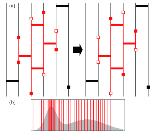
Figure S5: a, An illustration of the SSE cluster update process where the cluster marked in red is identified and flipped as a whole. A vertical line shows a spin expanded. The solid and empty squares show the diagonal and off-diagonal site operators. The solid bars show the diagonal bond operators. b, An illustration of the parametrization of a continuous spectral function into discrete $\delta$-functions.

9 Stochastic analytical continuation (SAC)

For the spectra in this paper we adopted a stochastic analytical continuation (SAC) [53, 54, 55] method to obtain the spectral function $S(\omega)$ from the imaginary time correlation $G(\tau)$ measured from QMC, which is generally believed a numerically unstable problem. This method will be briefly introduced below.

The spectral function $S(\omega)$ is connected to the imaginary time Green’s function $G(\tau)$ through an integral equation

$$G(\tau)=\int_{-\infty}^{\infty}\mathrm{d}\omega S(\omega)K(\tau,\omega)$$ (S14)

where $K(\tau,\omega)$ is the kernel function depending on the temperature and the statistics of the particles. We restrict ourselves to the case of spin systems and with only positive frequencies in the spectral, where $K(\tau,\omega)=(e^{-\tau\omega}+e^{-(\beta-\tau)\omega})/\pi$. To ensure the normalization of spectral function, we further modify the transformation and come to the following equation :

$$G(\tau)=\int_{0}^{\infty}\frac{\mathrm{d}\omega}{\pi}\frac{e^{-\tau\omega}+e^{-(\beta-\tau)\omega}}{1+e^{-\beta\omega}}B(\omega)$$ (S15)

where $B(\omega)=S(\omega)(1+e^{-\beta\omega})$ is the renormalized spectral function.

In practice, $G(\tau)$ for a set of imaginary time $\tau_{i}(i=1,\cdots N_{\tau})$ is measured in QMC simulation together with the statistical errors. The renormalized spectral function is parameterized into large number of equal-amplitude $\delta$-functions whose positions are sampled (Fig. S5b)

$$B(\omega)=\sum_{i=0}^{N_{\omega}}a_{i}\delta(\omega-\omega_{i})$$ (S16)

Then the fitted Green’s functions $\tilde{G}_{i}$ from Eq. S15 and the measured Greens functions $\bar{G}_{i}$ are compared by the fitting goodness

$$\chi^{2}=\sum_{i,j=1}^{N_{\tau}}(\tilde{G}_{i}-\bar{G}_{i})(C^{-1})_{ij}(\tilde{G}_{j}-\bar{G}_{j})$$ (S17)

where the covariance matrix is defined as

$$C_{ij}=\frac{1}{N_{B}(N_{B}-1)}\sum_{b=1}^{N_{B}}(G_{i}^{b}-\bar{G}_{i})(G_{j}^{b}-\bar{G}_{j}),$$ (S18)

with $N_{B}$ the number of bins, the measured Green’s functions of each $G_{i}^{b}$.

A Metropolis process is utilized to update the series in sampling. The weight for a given spectrum is taken to follow a Boltzmann distribution

$$W(\{a_{i},\omega_{i}\})\sim\exp\left(-\frac{\chi^{2}}{2\Theta}\right)$$ (S19)

with $\Theta$ a virtue temperature to balance the goodness of fitting $\chi^{2}$ and the smoothness of the spectral function. All the spectral functions of sampled series $\{a_{i},\omega_{i}\}$ is then averaged to obtain the spectrum as the final result.

References

- Endres et al. [2016] M. Endres, H. Bernien, A. Keesling, H. Levine, E. R. Anschuetz, A. Krajenbrink, C. Senko, V. Vuletic, M. Greiner, and M. D. Lukin, Atom-by-atom assembly of defect-free one-dimensional cold atom arrays, Science 354, 1024 (2016).
- Barredo et al. [2018] D. Barredo, V. Lienhard, S. de Léséleuc, T. Lahaye, and A. Browaeys, Synthetic three-dimensional atomic structures assembled atom by atom, Nature 561, 79 (2018).
- Bluvstein et al. [2021] D. Bluvstein, A. Omran, H. Levine, A. Keesling, G. Semeghini, S. Ebadi, T. T. Wang, A. A. Michailidis, N. Maskara, W. W. Ho, S. Choi, M. Serbyn, M. Greiner, V. Vuletić, and M. D. Lukin, Controlling quantum many-body dynamics in driven Rydberg atom arrays, Science 371, 1355 (2021).
- Browaeys and Lahaye [2020] A. Browaeys and T. Lahaye, Many-body physics with individually controlled Rydberg atoms, Nat. Phys. 16, 132 (2020).
- Jaksch et al. [2000] D. Jaksch, J. I. Cirac, P. Zoller, S. L. Rolston, R. Côté, and M. D. Lukin, Fast quantum gates for neutral atoms, Phys. Rev. Lett. 85, 2208 (2000).
- Lukin et al. [2001] M. D. Lukin, M. Fleischhauer, R. Cote, L. M. Duan, D. Jaksch, J. I. Cirac, and P. Zoller, Dipole blockade and quantum information processing in mesoscopic atomic ensembles, Phys. Rev. Lett. 87, 037901 (2001).
- Browaeys et al. [2016] A. Browaeys, D. Barredo, and T. Lahaye, Experimental investigations of dipole–dipole interactions between a few Rydberg atoms, J. Phys. B: At. Mol. Opt. Phys. 49, 152001 (2016).
- Kogut [1979a] J. B. Kogut, An introduction to lattice gauge theory and spin systems, Rev. Mod. Phys. 51, 659 (1979a).
- Samajdar et al. [2021a] R. Samajdar, W. W. Ho, H. Pichler, M. D. Lukin, and S. Sachdev, Quantum phases of Rydberg atoms on a kagome lattice, Proc. Natl. Acad. Sci. 118, e2015785118 (2021a).
- Samajdar et al. [2022] R. Samajdar, D. G. Joshi, Y. Teng, and S. Sachdev, Emergent gauge theories and topological excitations in Rydberg atom arrays, arXiv preprint arXiv:2204.00632 10.48550/arXiv.2204.00632 (2022).
- Yan et al. [2022] Z. Yan, R. Samajdar, Y.-C. Wang, S. Sachdev, and Z. Y. Meng, Triangular lattice quantum dimer model with variable dimer density, Nat. Commun. 13, 5799 (2022).
- Balents [2010] L. Balents, Spin liquids in frustrated magnets, Nature 464, 199 (2010).
- Savary and Balents [2016] L. Savary and L. Balents, Quantum spin liquids: a review, Rep. Prog. Phys. 80, 016502 (2016).
- Zhou et al. [2017] Y. Zhou, K. Kanoda, and T.-K. Ng, Quantum spin liquid states, Rev. Mod. Phys. 89, 025003 (2017).
- Kitaev [2006] A. Kitaev, Anyons in an exactly solved model and beyond, Ann. Phys. 321, 2 (2006).
- Grover and Senthil [2011] T. Grover and T. Senthil, Non-abelian spin liquid in a spin-one quantum magnet, Phys. Rev. Lett. 107, 077203 (2011).
- Semeghini et al. [2021] G. Semeghini, H. Levine, A. Keesling, S. Ebadi, T. T. Wang, D. Bluvstein, R. Verresen, H. Pichler, M. Kalinowski, R. Samajdar, et al., Probing topological spin liquids on a programmable quantum simulator, Science 374, 1242 (2021).
- Kogut [1979b] J. B. Kogut, An introduction to lattice gauge theory and spin systems, Rev. Mod. Phys. 51, 659 (1979b).
- Moessner and Raman [2011] R. Moessner and K. S. Raman, Quantum dimer models, in Introduction to Frustrated Magnetism (Springer, 2011) pp. 437–479.
- Fradkin et al. [2004] E. Fradkin, D. A. Huse, R. Moessner, V. Oganesyan, and S. L. Sondhi, Bipartite Rokhsar–Kivelson points and Cantor deconfinement, Phys. Rev. B 69, 224415 (2004).
- Vishwanath et al. [2004] A. Vishwanath, L. Balents, and T. Senthil, Quantum criticality and deconfinement in phase transitions between valence bond solids, Phys. Rev. B 69, 224416 (2004).
- Zhou et al. [2020] Z. Zhou, D.-X. Liu, Z. Yan, Y. Chen, and X.-F. Zhang, Quantum tricriticality of incommensurate phase induced by quantum domain walls in frustrated Ising magnetism (2020), arXiv:2005.11133 .
- Senthil et al. [2004] T. Senthil, A. Vishwanath, L. Balents, S. Sachdev, and M. P. A. Fisher, Deconfined quantum critical points, Science 303, 1490 (2004).
- Wang et al. [2017] C. Wang, A. Nahum, M. A. Metlitski, C. Xu, and T. Senthil, Deconfined quantum critical points: Symmetries and dualities, Phys. Rev. X 7, 031051 (2017).
- Celi et al. [2020] A. Celi, B. Vermersch, O. Viyuela, H. Pichler, M. D. Lukin, and P. Zoller, Emerging two-dimensional gauge theories in Rydberg configurable arrays, Phys. Rev. X 10, 021057 (2020).
- Fradkin and Kivelson [1990] E. Fradkin and S. Kivelson, Short range resonating valence bond theories and superconductivity, Mod. Phys. Lett. B 04, 225 (1990).
- Moessner et al. [2001a] R. Moessner, S. L. Sondhi, and P. Chandra, Phase diagram of the hexagonal lattice quantum dimer model, Phys. Rev. B 64, 144416 (2001a).
- Schlittler et al. [2015] T. Schlittler, T. Barthel, G. Misguich, J. Vidal, and R. Mosseri, Phase diagram of an extended quantum dimer model on the hexagonal lattice, Phys. Rev. Lett. 115, 217202 (2015).
- Yan et al. [2021] Z. Yan, Z. Zhou, O. F. Syljuåsen, J. Zhang, T. Yuan, J. Lou, and Y. Chen, Widely existing mixed phase structure of the quantum dimer model on a square lattice, Phys. Rev. B 103, 094421 (2021).
- Ran et al. [2022] X. Ran, Z. Yan, Y.-C. Wang, J. Rong, Y. Qi, and Z. Y. Meng, Fully packed quantum loop model on the square lattice: phase diagram and application for Rydberg atoms, arXiv preprint arXiv:2209.10728 10.48550/arXiv.2209.10728 (2022).
- Zhou et al. [2022] Z. Zhou, C. Liu, Z. Yan, Y. Chen, and X.-F. Zhang, Quantum dynamics of topological strings in a frustrated Ising antiferromagnet, npj Quantum Mater. 7, 60 (2022).
- Yan et al. [2021] Z. Yan, Z. Zhou, Y.-C. Wang, X. Qiu, Z. Y. Meng, and X.-F. Zhang, Preparing state within target topological sector of lattice gauge theory model on quantum simulator, arXiv e-prints , arXiv:2105.07134 (2021), arXiv:2105.07134 [quant-ph] .
- Scholl et al. [2021] P. Scholl, M. Schuler, H. J. Williams, A. A. Eberharter, D. Barredo, K.-N. Schymik, V. Lienhard, L.-P. Henry, T. C. Lang, T. Lahaye, et al., Quantum simulation of 2D antiferromagnets with hundreds of Rydberg atoms, Nature 595, 233 (2021).
- Li et al. [2022] C.-X. Li, S. Yang, and J.-B. Xu, Quantum phases of Rydberg atoms on a frustrated triangular-lattice array, Opt. Lett. 47, 1093 (2022).
- Villain, J. et al. [1980] Villain, J., Bidaux, R., Carton, J.-P., and Conte, R., Order as an effect of disorder, J. Phys. France 41, 1263 (1980).
- Moessner et al. [2000] R. Moessner, S. L. Sondhi, and P. Chandra, Two-dimensional periodic frustrated Ising models in a transverse field, Phys. Rev. Lett. 84, 4457 (2000).
- Moessner and Sondhi [2001] R. Moessner and S. L. Sondhi, Ising models of quantum frustration, Phys. Rev. B 63, 224401 (2001).
- Isakov and Moessner [2003] S. V. Isakov and R. Moessner, Interplay of quantum and thermal fluctuations in a frustrated magnet, Phys. Rev. B 68, 104409 (2003).
- Koziol et al. [2019] J. Koziol, S. Fey, S. C. Kapfer, and K. P. Schmidt, Quantum criticality of the transverse-field ising model with long-range interactions on triangular-lattice cylinders, Phys. Rev. B 100, 144411 (2019).
- Samajdar et al. [2021b] R. Samajdar, W. W. Ho, H. Pichler, M. D. Lukin, and S. Sachdev, Quantum phases of Rydberg atoms on a kagome lattice, Proc. Natl. Acad. Sci. 118, e2015785118 (2021b).
- [41] See Supplemental Material for a discussion of further details on the height field representation, the effective field theory around the RK point, the finite size scaling, the histogram and the correlation functions of order parameters, the excitation spectra, the intermediate regime, and the numerical methods of SSE and SAC .
- Jau et al. [2016] Y.-Y. Jau, A. M. Hankin, T. Keating, I. H. Deutsch, and G. W. Biedermann, Entangling atomic spins with a Rydberg-dressed spin-flip blockade, Nat. Phys. 12, 71 (2016).
- Sandvik [1997] A. W. Sandvik, Finite-size scaling of the ground-state parameters of the two-dimensional Heisenberg model, Phys. Rev. B 56, 11678 (1997).
- Sandvik [2003] A. W. Sandvik, Stochastic series expansion method for quantum Ising models with arbitrary interactions, Phys. Rev. E 68, 056701 (2003).
- Avella and Mancini [2013] A. Avella and F. Mancini, Strongly correlated systems: numerical methods, Vol. 176 (Springer, Berlin, 2013).
- Rokhsar and Kivelson [1988] D. S. Rokhsar and S. A. Kivelson, Superconductivity and the quantum hard-core dimer gas, Phys. Rev. Lett. 61, 2376 (1988).
- Henley [1997] C. L. Henley, Relaxation time for a dimer covering with height representation, J. Stat. Phys. 89, 483 (1997).
- Moessner et al. [2001b] R. Moessner, S. L. Sondhi, and E. Fradkin, Short-ranged resonating valence bond physics, quantum dimer models, and Ising gauge theories, Phys. Rev. B 65, 024504 (2001b).
- Stephenson [1966] J. Stephenson, Ising model spin correlations on the triangular lattice. ii. fourth‐order correlations, J. Math. Phys. 7, 1123 (1966).
- Polyakov [1977] A. Polyakov, Quark confinement and topology of gauge theories, Nucl. Phys. B 120, 429 (1977).
- Assaraf et al. [2000] R. Assaraf, M. Caffarel, and A. Khelif, Diffusion Monte Carlo methods with a fixed number of walkers, Phys. Rev. E 61, 4566 (2000).
- Syljuåsen [2005] O. F. Syljuåsen, Continuous-time diffusion Monte Carlo method applied to the quantum dimer model, Phys. Rev. B 71, 020401 (2005).
- Sandvik [1998] A. W. Sandvik, Stochastic method for analytic continuation of quantum Monte Carlo data, Phys. Rev. B 57, 10287 (1998).
- Shao et al. [2017] H. Shao, Y. Q. Qin, S. Capponi, S. Chesi, Z. Y. Meng, and A. W. Sandvik, Nearly deconfined spinon excitations in the square-lattice spin- Heisenberg antiferromagnet, Phys. Rev. X 7, 041072 (2017).
- Sandvik [2016] A. W. Sandvik, Constrained sampling method for analytic continuation, Phys. Rev. E 94, 063308 (2016).
- Läuchli et al. [2008] A. M. Läuchli, S. Capponi, and F. F. Assaad, Dynamical dimer correlations at bipartite and non-bipartite Rokhsar-Kivelson points, J. Stat. Mech. 2008, P01010 (2008).
- Moessner and Sondhi [2003] R. Moessner and S. L. Sondhi, Three-dimensional resonating-valence-bond liquids and their excitations, Phys. Rev. B 68, 184512 (2003).
- Hermele et al. [2004] M. Hermele, M. P. A. Fisher, and L. Balents, Pyrochlore photons: The spin liquid in a three-dimensional frustrated magnet, Phys. Rev. B 69, 064404 (2004).
- Savary and Balents [2017] L. Savary and L. Balents, Disorder-induced quantum spin liquid in spin ice pyrochlores, Phys. Rev. Lett. 118, 087203 (2017).
- Wan and Tchernyshyov [2012] Y. Wan and O. Tchernyshyov, Quantum strings in quantum spin ice, Phys. Rev. Lett. 108, 247210 (2012).
- Blote and Hilborst [1982] H. W. J. Blote and H. J. Hilborst, Roughening transitions and the zero-temperature triangular Ising antiferromagnet, J. Phys. A 15, L631 (1982).
- Fisher and Stephenson [1963] M. E. Fisher and J. Stephenson, Statistical mechanics of dimers on a plane lattice. II. dimer correlations and monomers, Phys. Rev. 132, 1411 (1963).