Abstract

The rich multifractal properties of fluid turbulence illustrated by the work of Parisi and Frisch are related explicitly to Leray’s weak solutions of the three-dimensional Navier-Stokes equations. Directly from this correspondence it is found that the set on which energy dissipates, $\mathbb{F}_{m}$, has a range of dimensions $\mathfrak{D}_{m}=3/m$ ($1\leq m\leq\infty$), and a corresponding range of sub-Kolmogorov dissipation inverse length scales $L\eta_{m}^{-1}\leq Re^{3/(1+\mathfrak{D}_{m})}$ spanning $Re^{3/4}$ to $Re^{3}$. Correspondingly, the multifractal model scaling parameter $h$, must obey $h\geq h_{min}$ with $-{\scriptstyle\frac{2}{3}}\leq h_{min}\leq{\scriptstyle\frac{1}{3}}$.

In memory of Charlie Doering (1956-2021)

1 The need for a mathematical telescope

Despite the cliché that “turbulence is the last great unsolved problem in classical physics” [1], the challenge that it poses to physicists, mathematicians and engineers remains [2, 3, 4, 5, 6, 7, 8, 9, 10, 11, 12, 13, 14, 15, 16, 17, 18, 19]. A natural correspondence is proposed that helps us relate the rich multifractality of the statistical properties of homogeneous and isotropic fluid turbulence [2, 3, 4] to the methods of mathematical analysis which are used to study weak solutions of the incompressible Navier-Stokes equations [20, 21, 22, 24, 23, 25, 26, 27, 28], including the Millenial regularity problem [29]. Heretofore the two approaches have taken divergent paths which has caused a lacuna in our understanding. Multifractality is manifest in the wide sweep of vortical structures that appear in turbulent flows, ranging from three-dimensional vortices at many scales, to semi-broken filaments whose fractal dimension is less than unity : see Fig. 1 for illustrative examples. In telescopic terms, the simultaneous existence of many vortical structures each with its own fractal dimension requires the mathematical equivalent of an adjustable focus, somewhat in the manner of a zoom lens. Thus, an adjustable parameter with a wide range of values is needed. The multifractal model (MFM) of Parisi and Frisch possesses this latter feature through the allowed variation of its scaling parameter $h$ [2], while the Navier-Stokes equations seemingly do not. The MFM was developed after it had become clear that Kolmogorov’s 1941 theory needed to be modified in order to take account of the effects of intermittency [3] : see also [30, 31, 32, 33, 34, 35].

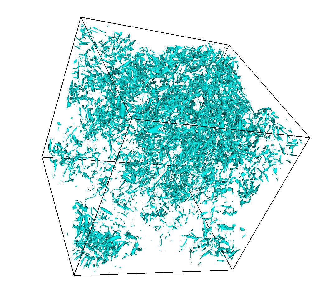
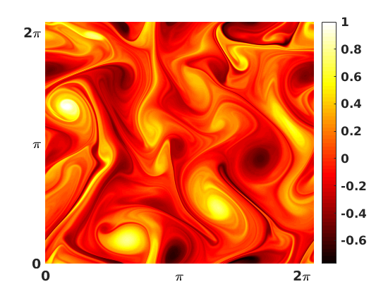
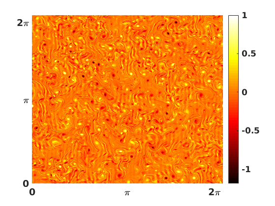
Figure 1: (left) Iso-surface plot of the magnitude of the vorticity $|\mbox{\boldmath$\omega$}|$ (two standard deviations above the mean) from a $512^{3}$ pseudospectral direct numerical simulation of the unforced $3D$ Navier-Stokes equations at a representative time at an integral-scale Reynolds number of 874. Plot courtesy of Nadia B. Padhan, IISc, Bangalore. The second and third are filled-contour plots of the vorticity from $2048^{2}$ pseudospectral direct numerical simulations of the forced $2D$ Navier-Stokes equations in a statistically steady state, courtesy of Kiran Kolluru, IISc, Bangalore : (middle) forward-cascade-dominated turbulence ($Re_{\lambda}=1957$) ; (right) inverse-cascade-dominated turbulence ($Re_{\lambda}=1729$).

The question is this : can this telescopic property be derived from Leray’s weak solution formulation of the three-dimensional incompressible Navier-Stokes equations [20, 21, 22, 24, 23, 25, 26, 27, 28]? From the Navier-Stokes side of the fence, no mathematical tools seemingly exist that would allow us to perform rigorous analysis on fractal sets. Standard methods of Navier-Stokes analysis involve integration over the full domain volume, which has the unfortunate consequence of washing out the delicate nature of the set on which energy dissipates [5, 6]. This paper circumvents these problems by showing how the existence of a multifractal set on which energy dissipates is natural to the problem. Results can be extracted from the Leray formalism which are then compared to the multifractal theory of Parisi and Frisch [2].

In recent work, Dubrulle and Gibbon [36] addressed the issue of the equivalence of the Navier-Stokes equations and the multifractal model. They used the Paladin-Vulpiani [32, 33] inverse dissipation length scale

$$L\eta^{-1}_{PV}\sim Re^{1/(1+h)}$$ (1.1)

as an ad hoc bridge between the two theories, where $h$ is the multifractal scaling parameter. In this paper we are able to go a step further by showing that this scale, at least in an inequality form, appears naturally out of the correspondence between the two theories without any ad hoc introduction.

2 Recasting Leray’s weak solution formulation of the Navier-Stokes equations

2.1 A zoom lens

The incompressible Navier-Stokes equations are

$$\left(\partial_{t}+\mbox{\boldmath$u$}\cdot\nabla\right)\mbox{\boldmath$u$}+\nabla p=\nu\Delta\mbox{\boldmath$u$}+\mbox{\boldmath$f$}(\mbox{\boldmath$x$})$$ (2.1)

subject to $\mbox{div}\,\mbox{\boldmath$u$}=\mbox{div}\,\mbox{\boldmath$f$}=0$, on a periodic domain $V_{d}=[0,\,L]^{d}$ for dimensions $d=3,\,2,\,1$. Results on weak solutions can be expressed in many ways [20] but most appear in time averaged form [21, 22, 24, 23, 25, 26, 27, 28]. In [27], it was shown that for $1\leq m\leq\infty$, the Sobolev norms

$$\|\nabla^{n}\mbox{\boldmath$u$}\|_{2m}=\left(\int_{V_{d}}|\nabla^{n}\mbox{\boldmath$u$}|^{2m}\,dV\right)^{1/2m}\,,$$ (2.2)

under the Navier-Stokes invariance property $\mbox{\boldmath$x$}^{\prime}=\lambda^{-1}\mbox{\boldmath$x$}$ ; $t^{\prime}=\lambda^{-2}t$ and $\mbox{\boldmath$u$}=\lambda^{-1}\mbox{\boldmath$u$}^{\prime}$, have the scaling property

$$\|\nabla^{n}\mbox{\boldmath$u$}\|_{2m} = \lambda^{-1/\alpha_{n,m,d}}\|\nabla^{{}^{\prime}n}\mbox{\boldmath$u$}^{\prime}\|_{2m}\,$$ (2.3)

$$\alpha_{n,m,d} = \frac{2m}{2m(n+1)-d}\,.$$ (2.4)

It has been shown in [27, 28] that for $n\geq 1$, the weighted time averages of the dimensionless family

$$F_{n,m,d}=\nu^{-1}L^{1/\alpha_{n,m,d}}\|\nabla^{n}\mbox{\boldmath$u$}\|_{2m}$$ (2.5)

are finite such that

$$\left<F_{n,m,d}^{(4-d)\alpha_{n,m,d}}\right>_{T}<\infty\,.$$ (2.6)

The brackets $\left<\cdot\right>_{T}$ are a time average up to time $T>0$. The set of exponents $\alpha_{n,m,d}$ in (2.6) clearly play a significant role in Navier-Stokes regularity properties. A series of well known weak solution results can be recovered by choosing various values of $n$ and $m$, which all have the same level of regularity [27]. Increasing $m$ amplifies the larger features in the solution in proportion to the smaller until $m=\infty$ is reached which corresponds to the maximum. Therefore, adjusting the value of $m$ acts as a focus control on a telescope that allows us to zoom into different features in a landscape. The subscript labelling on $\alpha_{n,m,d}$ encodes the nature of the norm of which it is an exponent : thus $(n,m,d)$ means “$n$ derivatives in $L^{2m}$ in integer-$d$ spatial dimensions”. However, $\alpha_{n,m,d}$ can be rewritten as

$$\alpha_{n,m,d} = \frac{2}{2(n+1)-\mathfrak{D}_{m}}\,,\qquad\mathfrak{D}_{m}=d/m\,,$$ (2.7)

$$= \alpha_{n,1,\mathfrak{D}_{m}}\,.$$

The subscripts on $\alpha_{n,1,\mathfrak{D}_{m}}$ now suggest that the problem can now be recast into “$n$ derivatives in $L^{2}$ on a set, designated as $\mathbb{F}_{m}$, which has a range of dimensions $\mathfrak{D}_{m}=d/m$”. The range of dimensions $\mathfrak{D}_{m}=d/m$ suggests that $\mathbb{F}_{m}$ is multifractal in character, with a corresponding set of co-dimensions

$$\mathfrak{C}_{m}=d\left(1-\frac{1}{m}\right)\,.$$ (2.8)

Mimicking (2.6), the recasting of $\alpha_{n,m,d}$ into $\alpha_{n,1,\mathfrak{D}_{m}}$ suggests that the family of time averages

$$X_{n,\mathfrak{D}_{m}}(T)=\left<F_{n,1,\mathfrak{D}_{m}}^{(4-\mathfrak{D}_{m})\,\alpha_{n,1,\mathfrak{D}_{m}}}\right>_{T}\,,$$ (2.9)

may be a key set of objects. The $X_{n,m,\mathfrak{D}_{m}}$ are neither necessarily equal to the averages in (2.6) nor would it be an easy task to prove they are bounded above because there exists no mechanism for performing analysis on fractal or multifractal domains. Nevertheless, the case $n=1$ is an exception in that it can be bounded because of the cancellation of the factor of $(4-\mathfrak{D}_{m})$ in

$$\left[(4-\mathfrak{D}_{m})\alpha_{n,1,\mathfrak{D}_{m}}\right]_{n=1}=2\,,\qquad 1\leq m\leq\infty\,,$$ (2.10)

for every value of $0\leq\mathfrak{D}_{m}\leq d$. It is this case we consider in the next subsection.

2.2 The three-dimensional case when $n=1$

The $n=1$ case of (2.9) for $d=3$ corresponds, for each $m$, to a time-averaged energy dissipation rate $\varepsilon_{m}$ on the multifractal set $\mathbb{F}_{m}$. Each $\varepsilon_{m}$ is defined as

$$\varepsilon_{m}=\nu L^{-\mathfrak{D}_{m}}\left<\int_{\mathbb{F}_{m}}|\nabla\mbox{\boldmath$u$}|^{2}dV\right>_{T}\,,\quad\mathfrak{D}_{m}=3/m\,.$$ (2.11)

Noting that $\mathbb{F}_{m}\subset\mathbb{T}^{3}$, (2.11) can be re-written as

$$\varepsilon_{m} \leq \nu L^{3-\mathfrak{D}_{m}}L^{-3}\left<\int_{\mathbb{T}^{3}}|\nabla\mbox{\boldmath$u$}|^{2}dV\right>_{T}$$ (2.12)

$$\leq c\,L^{-1-\mathfrak{D}_{m}}\nu^{3}Re^{3}\,.$$

The $Re^{3}$ upper bound is derived for generic narrow-band forcing considered by Doering and Foias [16] where the Reynolds number $Re$ is defined by

$$Re=UL/\nu\qquad\mbox{with}\qquad U^{2}=L^{-3}\left<\|\mbox{\boldmath$u$}\|^{2}_{2}\right>_{T}\,.$$ (2.13)

(2.12) shows that $\varepsilon_{m}\nu^{-3}$ can be expressed in terms of a set of inverse lengths $\eta_{m}^{-1}$ defined such that

$$\varepsilon_{m}\nu^{-3}:=\eta_{m}^{-1-\mathfrak{D}_{m}}$$ (2.14)

leading to

$$L\eta_{m}^{-1}\leq c\,Re^{\frac{3}{1+\mathfrak{D}_{m}}}\,.$$ (2.15)

(2.15) is a formula that appears in Kraichnan [31], but without any identification of the nature of $\mathbb{F}_{m}$. The size of the upper bound on $L\eta_{m}^{-1}$ ranges from the standard inverse Kolmogorov bound $Re^{3/4}$ when $m=1$ to $Re^{3}$ when $m=\infty$.

2.3 The two-dimensional case

What of the two-dimensional case? Advantage can be taken of the lack of a vortex stretching term ($\mbox{\boldmath$\omega$}\cdot\nabla\mbox{\boldmath$u$}=0$) in the vorticity formulation to find the enstrophy dissipation rate [16, 5]

$$\nu L^{-2}\left<\int_{\mathbb{T}^{2}}|\nabla\mbox{\boldmath$\omega$}|^{2}dV\right>_{T}\leq c\,\nu^{3}L^{-6}Re^{3}\,.$$ (2.16)

In a full $\mathbb{T}^{2}$ domain, (2.16) leads to an $Re^{1/2}$ bound on the set of inverse Kraichnan lengths $L\eta_{m,ens}^{-1}$. The equivalent of (2.11) for the enstrophy dissipation rate on $\mathbb{F}_{m}$ is

$$\varepsilon_{m,ens}=\nu L^{-\mathfrak{D}_{m}}\left<\int_{\mathbb{F}_{m}}|\nabla\mbox{\boldmath$\omega$}|^{2}dV\right>_{T}\,,$$ (2.17)

with $\mathfrak{D}_{m}=2/m$. Then $\varepsilon_{m,ens}\nu^{-3}$ can be expressed in terms of a set of inverse lengths $\eta_{m,ens}^{-1}$ such that $\varepsilon_{m,ens}\nu^{-3}=\eta_{m,ens}^{-4-\mathfrak{D}_{m}}$, leading to

$$L\eta_{m,ens}^{-1}\leq c\,Re^{\frac{3}{4+\mathfrak{D}_{m}}}\,,$$ (2.18)

and thus a spread of $Re^{1/2}$ to $Re^{3/4}$. In this two-dimensional case Alexakis and Doering [17] derived a tighter bound of $Re^{2}$ on the right hand side of (2.16) when the forcing has a single wave-number or has a constant flux. An amendation of the numerator in (2.18) gives a spread ranging from $Re^{1/3}$ to $Re^{1/2}$, thus implying even less multifractality.

3 Correspondence with the multifractal model

Kolmogorov’s 1941 theory (K41) of three-dimensional, homogeneous, isotropic turbulence [3] revolves around the $p$th-order velocity structure function $S_{\!p}$ defined as

$$S_{\!p}=\left<\left|\mbox{\boldmath$u$}(\mbox{\boldmath$x$}+\mbox{\boldmath$r$})-\mbox{\boldmath$u$}(\mbox{\boldmath$x$})\right|^{p}\right>_{stat.av.}\,.$$ (3.1)

The scaling properties of $S_{\!p}$ have their origin in the invariance property enjoyed by the incompressible Euler equations under the transformation $\mbox{\boldmath$x$}^{\prime}=\lambda^{-1}\mbox{\boldmath$x$}$ ; $t^{\prime}=\lambda^{h-1}t$ and $\mbox{\boldmath$u$}=\lambda^{h}\mbox{\boldmath$u$}^{\prime}$. The scaling parameter $h$ can take any value, unlike the Navier-Stokes equations where it must satisfy $h=-1$. The invariance property shows that $S_{\!p}$ scales as $S_{\!p}\sim r^{hp}$. As explained in [3], the axioms of K41 lead to $h={\scriptstyle\frac{1}{3}}$, which is consistent with the “four-fifths law” $S_{3}=-{\scriptstyle\frac{4}{5}}\varepsilon r$. The problem with the result $S_{\!p}\sim r^{p/3}$ is that experimental data deviate from the linear in $p$ scaling but instead lie on a concave curve $\zeta_{p}$ below the line ${\scriptstyle\frac{1}{3}}p$. The multifractal model of Parisi and Frisch [2, 3] adapted the K41 formalism by relaxing the requirement that $h={\scriptstyle\frac{1}{3}}$ by insisting that the energy dissipation rate is invariant in $h$ only in an average sense. They achieved this by introducing the probability $P(h)\sim r^{3-D(h)}$ of observing a given scaling exponent $h$ at the scale $r$. Each value of $h$ belongs to a given fractal set of dimension $D(h)$. This procedure produces the result

$$S_{\!p}\sim r^{\zeta_{p}}\quad\mbox{where}\quad\zeta_{p}=\min_{h}\left[hp+3-D(h)\right]\,.$$ (3.2)

This must be constrained by the four-fifths law which requires $\zeta_{3}=1$, thus leading to the inequalities for $D(h)$ and the co-dimension $C(h)$ (which sum to the spatial dimension)

$$D(h)\leq 3h+2\quad\Rightarrow\quad C(h)\geq 1-3h\,.$$ (3.3)

Given that K41 and the MFM models revolve around the flow being homogeneous and isotropic, any comparison with results from the Navier-Stokes equations will likely only be valid when the flow has reached a fully turbulent state : i.e. when $T$ is sufficiently large.

To make the two theories touch, it is natural to suggest a correspondence between $\mathfrak{D}_{m}$ and $D(h)$ and $\mathfrak{C}_{m}$ and $C(h)$, which leads to a simple inequality relating $m$ and $h$

$$\frac{3}{m}\leq 2+3h\,,$$ (3.4)

from which we find $h\geq h_{min}$ with $h_{min}=m^{-1}-{\scriptstyle\frac{2}{3}}$. The two opposite limits $m\to 1$ and $m\to\infty$ give

$$-{\scriptstyle\frac{2}{3}}\leq h_{min}\leq{\scriptstyle\frac{1}{3}}\,,$$ (3.5)

which is precisely the range found in [36].

A more modern version of the multifractal model uses the theory of large deviations to re-express $P(h)$ as $P(h)\sim r^{C(h)}$, where $C(h)$ is the multifractal spectrum [3, 35, 6]. $C(h)$ therefore plays the role as the co-dimension. In the theory of large deviations it is possible that $C(h)\geq 3$, the domain dimension, corresponding to $D(h)<0$, but only with an infinitesimal probability. This would correspond to $m<0$, which must be excluded here. The exponent $3/(1+\mathfrak{D}_{m})$ in (2.15) is bounded below by

$$\frac{3}{1+\mathfrak{D}_{m}}\geq\frac{1}{1+h}\,.$$ (3.6)

The left hand side of (3.6) is derived directly from the Navier-Stokes equations, while the right hand side comes from the MFM and can be recognized as the Paladin-Vulpiani inverse dissipation scale $\eta^{-1}_{PV}$ defined in (1.1). Paladin and Vulpiani [32] treated (3.3) as an equality, which would change the $\geq$ in (3.6) to equality. Thus we see that the Paladin-Vulpiani scale appears naturally in this formulation.

Finally, given that there exists a continuum of sub-Kolmogorov scales from the $n=1$ case alone, the role of higher derivatives ($n>1$) in the $X_{n,\mathfrak{D}_{m}}$ in (2.9) is an open question and one that is relevant to the regularity problem. Dubrulle and Gibbon [36] have shown that the lower bound on $C(h)\geq 1-3h$ holds for all values of $n$, meaning that one can do no better than the result given by the four-fifths law at $n=1$. In (3.5), $h\geq-{\scriptstyle\frac{2}{3}}$ bounds $h$ away from the dangerous value of $h=-1$, where real singularities can occur [37, 3, 35, 36]. Recent work in [38, 39] has characterized small structures using values of $h$.

Acknowledgments : The author thanks the Isaac Newton Institute for Mathematical Sciences, Cambridge for support and hospitality during the programme Mathematical Aspects of Fluid Turbulence : where do we stand? in 2022, when work on this paper was undertaken. This work was supported by EPSRC grant no EP/R014604/1&#34. Thanks are also due to Berengere Dubrulle (Saclay) and Dario Vincenzi (Nice) for discussions. I am indebted to Nadia Padhan and Kiran Kolluru of IISc Physics Department, Bangalore for the plots in Fig. 1.

References

- [1] K. Sreenivasan & G. Falkovich, Lessons from Hydrodynamic Turbulence, Physics Today, 59 (2006) 43–49.
- [2] G. Parisi and U. Frisch, in Turbulence and Predictability in Geophysical Fluid Dynamics. Proc. Int. School of Physics “E. Fermi” 1983 Varenna, Italy, edited by M. Ghil, R. Benzi and G. Parisi, pp. 84–87 North-Holland, (Amsterdam 1985).
- [3] U. Frisch, Turbulence : The Legacy of A. N. Kolmogorov, Cambridge University Press (Cambridge, 1995).
- [4] C. Meneveau and K. R. Sreenivasan, The multifractal nature of turbulent energy dissipation, J. Fluid Mech. 224 (1991) 429–484.
- [5] M. K. Verma, Energy transfer in fluid flows : Multiscale and Spectral Perspectives, Cambridge University Press (Cambridge, 2019).
- [6] B. Dubrulle, Beyond Kolmogorov cascades, J. Fluid Mech. 867 (2019) 1–63.
- [7] P. K. Yeung and K. Ravikumar, Advancing understanding of turbulence through extreme-scale computation : Intermittency and simulations at large problem sizes, Phys. Rev. Fluids 5 (2020) 110517.
- [8] G. E. Elsinga, T. Ishihara and J. C. R. Hunt, Extreme dissipation and intermittency in turbulence at very high Reynolds numbers, Proc. R. Soc. A 476 (2020) 20200591.
- [9] D. Buaria, A. Pumir, E. Bodenschatz, and P. K. Yeung, Extreme velocity gradients in turbulent flows, New J. Phys. 21 (2019) 043004.
- [10] T. Ishihara, K. Morishita, M. Yokokawa, A. Uno, and Y. Kaneda, Energy spectrum in high-resolution direct numerical simulation of turbulence, Phys. Rev. Fluids 1 (2016) 082403(R).
- [11] M. Buzzicotti, A. Bhatnagar, L. Biferale, A. Lanotte and S. S. Ray, Lagrangian statistics for Navier-Stokes turbulence under Fourier-mode reduction : fractal and homogeneous decimations, New J. Phys. 18 (2016) 113047.
- [12] D. A. Donzis, J. D. Gibbon, A. Gupta, R. M. Kerr, R. Pandit and D. Vincenzi, Vorticity moments in four numerical simulations of the Navier-Stokes equations, J. Fluid Mech. 732 (2013) 316–31.
- [13] K. R. Sreenivasan and C. Meneveau, The Fractal Facets of Turbulence, J. Fluid Mech. 173 (1986) 357–386.
- [14] S. Douady, Y. Couder and M. E. Brachet, Direct observation of the intermittency of intense vorticity filaments in turbulence, Phys. Rev. Lett. 67 (1991) 983–986.
- [15] E. Aurell, U. Frisch, J. Lutsko and M. Vergassola, On the multifractal properties of the energy dissipation derived from turbulence data, J. Fluid Mech. 238 (1992) 467–486.
- [16] C. R. Doering and C. Foias, Energy dissipation in body-forced turbulence, J. Fluid Mech. 467 (2002) 289–306.
- [17] A. Alexakis and C. R. Doering, Energy and enstrophy dissipation in steady state 2D turbulence, Phys. Letts. A 359 (2006) 652–657.
- [18] L. Chevillard, S. G. Roux, E. Leveque, N. Mordant, J. F. Pinton and A. Arneodo, Intermittency of velocity time increments in turbulence, Phys. Rev. Letts. 95 (2005) 064501.
- [19] T. Ishihara, T. Gotoh and Y. Kaneda, Study of high-Reynolds number isotropic turbulence by direct numerical simulation, Annu. Rev. Fluid Mech. 41 (2009) 165–180.
- [20] J. Leray, Sur le mouvement d’un liquide visqueux emplissant l’éspace, Acta Math. 63 (1934) 193–248.
- [21] C. Foias, C. Guillopé and R. Temam, New a priori estimates for Navier-Stokes equations in dimension 3, Comm. Part. Diff. Equns. 6(3) (1981) 329–359.
- [22] C. R. Doering and J. D. Gibbon, Applied Analysis of the Navier-Stokes Equations, Cambridge University Press (Cambridge, 1995).
- [23] C. Foias, O. Manley, R. Rosa and R. Temam, Navier-Stokes Equations and Turbulence, Cambridge University Press (Cambridge, 2001).
- [24] L. Escauriaza, G. Seregin and V. Sverak, On -Solutions to the Navier-Stokes equations and backward uniqueness, Russ. Math. Surveys 58 (2003) 211–262.
- [25] A. Cheskidov and R. Shvydkoy, A unified approach to regularity problems for the Navier-Stokes and Euler equations : the use of Kolmogorov’s dissipation range, J. Math. Fluid Mech. 16 (2014) 263–273.
- [26] J. C. Robinson, J. L. Rodrigo and W. Sadowski, The Three-dimensional Navier-Stokes Equations : Classical Theory ; Cambridge Studies in Advanced Mathematics, Cambridge University Press (Cambridge, 2016).
- [27] J. D. Gibbon, Weak and Strong Solutions of the 3D Navier-Stokes Equations and Their Relation to a Chessboard of Convergent Inverse Length Scales, J. Nonlin. Sci. 29(1) (2019) 215–228.
- [28] J. D. Gibbon, Intermittency, cascades and thin sets in three-dimensional Navier-Stokes turbulence, EPL 131 (2020) 64001.
- [29] https://www.claymath.org/millennium-problems/navier%E2%80%93stokes-equation
- [30] R. Benzi, G. Paladin, G. Parisi and A. Vulpiani, On the multifractal nature of fully developed turbulence and chaotic systems, J. Phys. A : Math. Gen. 17 (1984) 3521–3531.
- [31] R. H. Kraichnan, Intermittency and attractor size in isotropic turbulence, Phys. Fluids 28 (1985) 10–11.
- [32] G. Paladin and A. Vulpiani, Degrees of freedom of turbulence, Phys. Rev. A 35 (1987) 1971–1973.
- [33] G. Paladin and A. Vulpiani, Anomalous scaling laws in multifractal objects, Phys. Rep. 156 4 (1987) 147–225.
- [34] M. Nelkin, Multifractal scaling of velocity derivatives in turbulence, Phys. Rev. A 42 (1990) 7226–7229.
- [35] G. L. Eyink (2008) Turbulence Theory – unpublished lecture notes chapters 3c,d ; The Johns Hopkins University, Baltimore, http://www.ams.jhu.edu/~eyink/Turbulence/notes/
- [36] B. Dubrulle and J. D. Gibbon, A correspondence between the multifractal model of turbulence and the Navier–Stokes equations, Phil. Trans. R. Soc. A 380 (2022) 20210092.
- [37] L. Caffarelli, R. Kohn and L. Nirenberg, Partial regularity of suitable weak solutions of the Navier-Stokes equations, Comm. Pure Appl. Math. 35 (1982) 771–831.
- [38] F. Nguyen, J.-P. Laval, P. Kestener, A. Cheskidov, R. Shvydkoy and B. Dubrulle, Local estimates of Hölder exponents in turbulent vector fields, Phys. Rev. E 99 (2019) 053114.
- [39] F. Nguyen, J.-P. Laval and B. Dubrulle, Characterizing most irregular small-scale structures in turbulence using local Hölder exponents, Phys. Rev. E 102 (2020) 063105.