Numerical range for weighted Moore-Penrose inverse of tensor

Abstract

This article first introduces the notion of weighted singular value decomposition (WSVD) of a tensor via the Einstein product. The WSVD is then used to compute the weighted Moore-Penrose inverse of an arbitrary-order tensor. We then define the notions of weighted normal tensor for an even-order square tensor and weighted tensor norm. Finally, we apply these to study the theory of numerical range for the weighted Moore-Penrose inverse of an even-order square tensor and exploit its several properties. We also obtain a few new results in the matrix setting that generalizes some of the existing results as particular cases.

1 Introduction

The terms numerical range and numerical radius have drawn significant attention from the researchers in the last few decades in the field of matrix and operator theory [3, 4, 13, 14]. These have been widely studied because of their applications in many areas, such as numerical analysis and differential equations [1, 6, 9, 11, 12, 19, 23, 29]. The numerical range (or the field of values) of a square matrix $A\in\mathbb{C}^{n\times n}$ is a subset of complex numbers defined as:

$$W(A)=\{\left\langle Ax,x\right\rangle:\;x\in\mathbb{C}^{n},\|x\|=1\},$$ (1)

where $\left\langle x,y\right\rangle=y^{*}x$ for $x,y\in\mathbb{C}^{n}$ and $\|x\|=\left\langle x,x\right\rangle^{1/2}$. And, the numerical radius of the matrix $A$ is defined as:

$$w(A)=\textnormal{max}\{|z|:\;z\in W(A)\}.$$ (2)

One of the main reasons for emphasizing the numerical range concept is its many attractive properties. For example, $W(A)$ is a convex subset of $\mathbb{C}$ (known as Toeplitz-Hausdorff theorem [14]). Further, the numerical range of a matrix contains its spectrum (or the set of all eigenvalues). The numerical radius is frequently employed as a more reliable indicator of the rate of convergence of iterative methods than the spectral radius [1, 9]. In 2016, Ke et al. [18] introduced tensor numerical ranges using tensor inner products and tensor norms via the $k$-mode product, which may not be convex in general (see Example 1, [18]). In 2021, Pakmanesh and Afshin [28] continued the same study for even-order tensors and proved the convexity for the numerical range of an even-order tensor. In the same year, Rout et al. [30] introduced tensor numerical ranges using tensor inner products and tensor norms via the Einstein product. The authors [30] studied several fundamental notions of tensor numerical ranges, such as unitary invariance, spectral containment, and convexity. Furthermore, they developed an algorithm to plot the boundary of the numerical range of a tensor, which helps to design faster algorithms for the calculations of its eigenvalues. To understand tensor numerical ranges, we first recall some basic facts about tensors. Tensors are generalizations of scalars (that have no index), vectors (that have precisely one index), and matrices (that have precisely two indices) to an arbitrary number of indices. A tensor is represented as a multidimensional array. An $N^{th}$-order tensor is defined as:

$$\mathcal{A}=(a_{i_{1}i_{2}\ldots i_{N}})\in\mathbb{C}^{I_{1}\times\cdots\times I_{N}};~{}1\leq i_{k}\leq I_{k}~{}\textnormal{for each}~{}k=1,2,...,N,$$

where each mode $I_{k}$ is a natural number and the notation $a_{i_{1}\ldots i_{N}}$ represents an $(i_{1},\ldots,i_{N})^{th}$ element of $\mathcal{A}$. For simplicity, $I_{1}\times I_{2}\times\cdots\times I_{N}$ is also written as $I_{1\ldots N}$. The transpose of a tensor may not be unique, which is recalled here. Let $\mathcal{A}\in\mathbb{C}^{I_{1}\times I_{2}\times\cdots\times I_{M}}$ be a tensor and let $\pi$ be a permutation in $S_{M}$ except the identity permutation, where $S_{M}$ represents the permutation group over the set $\{1,2,\ldots,M\}$. Then, the $\pi$-transpose of the tensor $\mathcal{A}$ is defined as

$$\mathcal{A}^{T_{\pi}}=(a_{i_{\pi(1)}i_{\pi(2)}\ldots i_{\pi(M)}})\in\mathbb{C}^{I_{\pi(1)}\times I_{\pi(2)}\times\cdots\times I_{\pi(M)}}.$$ (3)

Thus, there are $M!-1$ possible transposes associated with a tensor $\mathcal{A}\in\mathbb{C}^{I_{1}\times I_{2}\times\cdots\times I_{M}}$. In particular, for $\mathcal{A}=(a_{i_{1}i_{2}\ldots i_{M}j_{1}j_{2}\ldots j_{N}})\in\mathbb{C}^{I_{1}\times I_{2}\times\cdots\times I_{M}\times J_{1}\times J_{2}\times\cdots\times J_{N}}$ and $\pi\in S_{M+N}$ such that $\mathcal{A}^{T_{\pi}}=(b_{j_{1}j_{2}\ldots j_{N}i_{1}i_{2}\ldots i_{M}})=(a_{i_{1}i_{2}\ldots i_{M}j_{1}j_{2}\ldots j_{N}})\in\mathbb{C}^{J_{1}\times J_{2}\times\cdots\times J_{N}\times I_{1}\times I_{2}\times\cdots\times I_{M}}$, then it is simply written as $\mathcal{A}^{T}$. Similarly, the conjugate transpose of $\mathcal{A}$ is denoted by $\mathcal{A}^{H}$ and defined by $\mathcal{A}^{H}=(c_{j_{1}j_{2}\ldots j_{N}i_{1}i_{2}\ldots i_{M}})=(\overline{a}_{i_{1}i_{2}\ldots i_{M}j_{1}j_{2}\ldots j_{N}})\in\mathbb{C}^{J_{1}\times J_{2}\times\cdots\times J_{N}\times I_{1}\times I_{2}\times\cdots\times I_{M}}$, where bar denotes the complex conjugate of a number. Furthermore, if $\mathcal{A}\in\mathbb{C}^{I_{1}\times I_{2}\times\cdots\times I_{M}}$, then $\mathcal{A}^{T}=(a_{1i_{1}i_{2}\ldots i_{M}})\in\mathbb{C}^{1\times I_{1}\times I_{2}\times\cdots\times I_{M}}$. There are two ways to define a square tensor. One when each mode is of equal size, i.e., $n\times n\times\cdots\times n$ and another when the first $N$ modes are repeated in the same order, i.e., $I_{1}\times I_{2}\times\cdots\times I_{N}\times I_{1}\times I_{2}\times\cdots\times I_{N}$. Ke et al. [18] extended the notion of the numerical range of a matrix for the former type of square tensors. Further, Rout et al. [30] extended the numerical range for the latter type of square tensors. They also obtained a few properties of tensor numerical range of the Moore–Penrose inverse via the Einstein product. We aim to study these properties of tensor numerical range for the weighted Moore-Penrose inverse of a tensor. For this purpose, we recall the Einstein product below.

The Einstein product [10] $\mathcal{A}*_{N}\mathcal{B}\in\mathbb{C}^{I_{1\ldots M}\times J_{1\ldots L}}$ of tensors $\mathcal{A}\in\mathbb{C}^{I_{1\ldots M}\times K_{1\ldots N}}$ and $\mathcal{B}\in\mathbb{C}^{K_{1\ldots N}\times J_{1\ldots L}}$ is defined by the operation $*_{N}$ via

$$(\mathcal{A}*_{N}\mathcal{B})_{i_{1}\ldots i_{M}j_{1}\ldots j_{L}}=\displaystyle\sum_{k_{1},\ldots,k_{N}}a_{{i_{1}\ldots i_{M}}{k_{1}\ldots k_{N}}}b_{{k_{1}\ldots k_{N}}{j_{1}\ldots j_{L}}}.$$

The associative law for the Einstein product holds. In the above formula, if $\mathcal{B}\in\mathbb{C}^{K_{1\ldots N}}$, then $\mathcal{A}*_{N}\mathcal{B}\in\mathbb{C}^{I_{1\ldots M}}$ and

$$(\mathcal{A}*_{N}\mathcal{B})_{i_{1}\ldots i_{M}}=\displaystyle\sum_{k_{1},\ldots,k_{N}}a_{{i_{1}\ldots i_{M}}{k_{1}\ldots k_{N}}}b_{{k_{1}\ldots k_{N}}}.$$

This product is used in the study of the theory of relativity [10] and in the area of continuum mechanics [21]. Let $A\in\mathbb{R}^{m\times n}$ and $B\in\mathbb{R}^{n\times l}$. Then, the Einstein product $*_{1}$ reduces to the standard matrix multiplication as

$$(A*_{1}B)_{ij}=\displaystyle\sum_{k=1}^{n}a_{ik}b_{kj}.$$

We refer to [15] for further advantages of studying the theory of tensors via the Einstein product. In 2019, Liang and Zheng [22] introduced the notion of the eigenvalues of an even-order square tensor via the Einstein product as follows.

Definition 1.1 (Definition 2.3, [22]).

Let $\mathcal{A}\in\mathbb{C}^{I_{1\ldots N}\times I_{1\ldots N}}$. Then, a complex number $\lambda$ is called an eigenvalue of $\mathcal{A}$ if there exists a nonzero tensor $\mathcal{X}\in\mathbb{C}^{I_{1\ldots N}}$ such that

$$\mathcal{A}*_{N}\mathcal{X}=\lambda\mathcal{X}.$$ (4)

The tensor $\mathcal{X}$ is called an eigentensor with respect to $\lambda$.

The set of all the eigenvalues of $\mathcal{A}$ is denoted by $\sigma(\mathcal{A})$. The spectral radius of the tensor $\mathcal{A}$ is denoted by $\rho(\mathcal{A})$ and defined by $\rho(\mathcal{A})=\max\{|\lambda|:\lambda\text{ is an eigenvalue of }\mathcal{A}\}.$ Furthermore, the positive square roots of eigenvalues of $\mathcal{A}^{H}*_{N}\mathcal{A}$ are called the singular values of $\mathcal{A}$. The maximum singular value of $\mathcal{A}$ is called the spectral norm [31] of the tensor $\mathcal{A}$. In 2013, Brazell et al. [5] first introduced the notion of the inverse of a tensor via the Einstein product. For $\mathcal{A}\in\mathbb{C}^{I_{1\ldots N}\times I_{1\ldots N}}$, if there exists a tensor $\mathcal{X}\in\mathbb{C}^{I_{1\ldots N}\times I_{1\ldots N}}$ such that $\mathcal{A}*_{N}\mathcal{X}=\mathcal{I}=\mathcal{X}*_{N}\mathcal{A}$, then the tensor $\mathcal{X}$ is called the inverse of the tensor $\mathcal{A}$ and it is denoted by $\mathcal{A}^{-1}$. In 2016, Sun et al. [33] formally introduced a generalized inverse called the Moore-Penrose inverse of an even-order tensor via the Einstein product. The authors [33] then used the Moore-Penrose inverse to find the minimum-norm least-squares solution of some multilinear systems. Panigrahy and Mishra [25], Stanimirović et al. [32], and Liang and Zheng [22] independently improved the definition of the Moore-Penrose inverse of an even-order tensor to a tensor of any order via the same product. In 2017, Ji and Wei [16] defined the weighted Moore-Penrose inverse for an even-order square tensor, and then in 2020, Behera et al. [2] extended the definition to an arbitrary-order tensor. The definition of the weighted Moore-Penrose inverse of an arbitrary-order tensor and one result are recalled here.

Definition 1.2 (Definition 8, [2]).

Let $\mathcal{A}\in\mathbb{C}^{I_{1\ldots M}\times J_{1\ldots N}}$, and $\mathcal{M}\in\mathbb{C}^{I_{1\ldots M}\times I_{1\ldots M}}$, $\mathcal{N}\in\mathbb{C}^{J_{1\ldots N}\times J_{1\ldots N}}$ be two Hermitian positive definite tensors. Then, the tensor $\mathcal{X}\in\mathbb{C}^{J_{1\ldots N}\times I_{1\ldots M}}$ is called the weighted Moore-Penrose inverse of $\mathcal{A}$ if it satisfies the following four tensor equations:

$$\mathcal{A}*_{N}\mathcal{X}*_{M}\mathcal{A} = \mathcal{A};$$ (5)

$$\mathcal{X}*_{M}\mathcal{A}*_{N}\mathcal{X} = \mathcal{X};$$ (6)

$$(\mathcal{M}*_{M}\mathcal{A}*_{N}\mathcal{X})^{H} = \mathcal{M}*_{M}\mathcal{A}*_{N}\mathcal{X};$$ (7)

$$(\mathcal{N}*_{N}\mathcal{X}*_{M}\mathcal{A})^{H} = \mathcal{N}*_{N}\mathcal{X}*_{M}\mathcal{A}.$$ (8)

It is denoted by $\mathcal{A}_{\mathcal{M},\mathcal{N}}^{{\dagger}}$. In particular, if $\mathcal{M}$ and $\mathcal{N}$ are the identity tensors, then $\mathcal{A}_{\mathcal{M},\mathcal{N}}^{{\dagger}}=\mathcal{A}^{{\dagger}}$, the Moore-Penrose inverse [25] of $\mathcal{A}.$

Theorem 1.3 (Theorem 4, [2]).

Let $\mathcal{A}\in\mathbb{C}^{I_{1\ldots M}\times J_{1\ldots N}}$, and $\mathcal{M}\in\mathbb{C}^{I_{1\ldots M}\times I_{1\ldots M}}$, $\mathcal{N}\in\mathbb{C}^{J_{1\ldots N}\times J_{1\ldots N}}$ be two Hermitian positive definite tensors. If $\tilde{\mathcal{A}}=\mathcal{M}^{1/2}*_{M}\mathcal{A}*_{N}\mathcal{N}^{-1/2}$, then

$$\mathcal{A}_{\mathcal{M},\mathcal{N}}^{{\dagger}}=\mathcal{N}^{-1/2}*_{N}\tilde{\mathcal{A}}^{{\dagger}}*_{M}\mathcal{M}^{1/2}.$$

This article aims to introduce the notions of WSVD of an arbitrary-order tensor, weighted normal tensor, and weighted tensor norm and to establish their various properties. Some of these are utilized to investigate a few properties of the numerical range for the weighted Moore-Penrose inverse of an even-order square tensor. The rest of this article is structured as follows to accomplish our objectives. In Section 2, we recall some preliminaries. Then, we provide the WSVD and some of its applications in Section 3. Section 4 defines the weighted normal tensor and discusses its several features. In Section 5, we talk about the weighted tensor norm. Finally, we utilize all these notions to collect some properties of the numerical range, which examine different relations between the numerical range of a tensor and its weighted Moore-Penrose inverse in Section 6.

2 Preliminaries

For two tensors $\mathcal{X},\mathcal{Y}\in\mathbb{C}^{I_{1\ldots N}}$, an inner product $\left\langle\mathcal{X},\mathcal{Y}\right\rangle$ is defined as $\left\langle\mathcal{X},\mathcal{Y}\right\rangle=\mathcal{Y}^{H}*_{N}\mathcal{X}$ and a norm induced by this inner product as $\|\mathcal{X}\|=\left\langle\mathcal{X},\mathcal{X}\right\rangle^{1/2}$. A tensor $\mathcal{X}\in\mathbb{C}^{I_{1\ldots N}}$ is called a unit tensor if $\|\mathcal{X}\|=1$. First, we recall the definition of the numerical range and some results from [30].

Definition 2.1 (Definition 2.1, [30]).

Let $\mathcal{A}\in\mathbb{C}^{I_{1\ldots N}\times I_{1\ldots N}}$. Then, the numerical range of $\mathcal{A}$ is denoted by $W(\mathcal{A})$ and defined by

$$W(\mathcal{A})=\{\left\langle\mathcal{A}*_{N}\mathcal{X},\mathcal{X}\right\rangle:\;\mathcal{X}\text{ is a unit tensor in }\mathbb{C}^{I_{1\ldots N}}\}.$$ (9)

With some elementary calculations, it can be shown that

$$W(\mathcal{A})=\left\{\frac{\left\langle\mathcal{A}*_{N}\mathcal{X},\mathcal{X}\right\rangle}{\|\mathcal{X}\|^{2}}:\;\mathcal{O}\neq\mathcal{X}\in\mathbb{C}^{I_{1\ldots N}}\right\},$$ (10)

where $\mathcal{O}$ is the zero tensor having all the entries are zero. The numerical radius for the same tensor is defined as:

$$w(\mathcal{A})=\textnormal{max}\{|z|:\;z\in W(\mathcal{A})\}.$$ (11)

Note that, in the above Definition 2.1 when $N=1$, it coincides with the numerical range of a matrix defined in (1).

Theorem 2.2 (Theorem 5.1, [30]).

Let $\mathcal{A}\in\mathbb{C}^{I_{1\ldots N}\times I_{1\ldots N}}$. Then, $\mathcal{A}$ is normal (resp. Hermitian) if and only if $\mathcal{A}^{{\dagger}}$ is normal (resp. Hermitian).

We now recall the definition of the weighted conjugate transpose of a tensor proposed by Behera et al. [2]

Definition 2.3 (Definition 9, [2]).

Let $\mathcal{A}\in\mathbb{C}^{I_{1\ldots M}\times J_{1\ldots N}}$. If $\mathcal{M}\in\mathbb{C}^{I_{1\ldots M}\times I_{1\ldots M}}$ and $\mathcal{N}\in\mathbb{C}^{J_{1\ldots N}\times J_{1\ldots N}}$ are two Hermitian positive definite tensors, then the tensor

$$\mathcal{A}_{\mathcal{M}\mathcal{N}}^{\#}=\mathcal{N}^{-1}*_{N}\mathcal{A}^{H}*_{M}\mathcal{M}$$ (12)

is called the weighted conjugate transpose of $\mathcal{A}$.

The following definitions of tensor reshaping are derived from [32]. In 2020, Stanimirović et al. [32] defined a bijective map ‘rsh’ from the tensor space ${\mathbb{C}}^{M_{1\cdots m}\times N_{1\cdots n}}$ into the matrix space ${\mathbb{C}}^{(M_{1}\cdot M_{2}\cdot\cdots\cdot M_{m})\times(N_{1}\cdot N_{2}\cdot\cdots\cdot N_{n})}$ as follows:

Definition 2.4 (Definition 3.1, [32]).

The reshaping operation transforms an arbitrary tensor $\mathcal{A}\in\mathbb{C}^{M_{1\ldots m}\times N_{1\ldots n}}$ into the matrix $A\in\mathbb{C}^{\bf{m}\times\bf{n}}$ using the Matlab function reshape as follows:

$$\textnormal{rsh}(\mathcal{A})=A=reshape(\mathcal{A},\bf{m},\bf{n}),$$

where ${\bf{m}}=M_{1}\cdot M_{2}\cdot\cdots\cdot M_{m}$ and ${\bf{n}}=N_{1}\cdot N_{2}\cdot\cdots\cdot N_{n}.$ The inverse reshaping is the mapping defined by

$$\textnormal{rsh}^{-1}(A)=\mathcal{A}=reshape(A,M_{1},\ldots,M_{m},N_{1},\ldots,N_{n}).$$

Further, rshrank($\mathcal{A}$)=rank(rsh($A$)), is defined as the rank of the tensor $\mathcal{A}$, in the same article [32]. For the Einstein product of two tensors, reshape map satisfies the following property given as Lemma 3.1 in [32].

Lemma 2.5 (Lemma 3.1, [32]).

Let $\mathcal{A}\in\mathbb{C}^{M_{1\ldots m}\times N_{1\ldots n}}$ and $\mathcal{B}\in\mathbb{C}^{N_{1\ldots n}\times P_{1\ldots p}}$ be given tensors. Then,

$$\textnormal{rsh}(\mathcal{A}*_{N}\mathcal{B})=\textnormal{rsh}(\mathcal{A})\textnormal{rsh}(\mathcal{B})=AB,$$

where $\textnormal{rsh}(\mathcal{A})=A\in\mathbb{C}^{\bf{m}\times\bf{n}}$, $\textnormal{rsh}(\mathcal{B})=B\in\mathbb{C}^{\bf{n}\times\bf{p}}$, ${\bf{m}}=M_{1}\cdot M_{2}\cdot\cdots\cdot M_{m}$, ${\bf{n}}=N_{1}\cdot N_{2}\cdot\cdots\cdot N_{n}$, and ${\bf{p}}=P_{1}\cdot P_{2}\cdot\cdots\cdot P_{p}.$

3 Weighted singular value decomposition

This section contains some of the main results of this article. We prove that any tensor can be decomposed into the tensor Einstein product of three special tensors. We call it the WSVD of the given tensor as it generalizes the notion of the WSVD of a matrix [35]. After that, we derive a formula to compute the weighted Moore-Penrose inverse of a given arbitrary-order tensor. For applications of the WSVD of a matrix, we refer [17, 20, 24, 34] and references therein. In particular, the WSVD is widely used in solving weighted least squares solutions [35, 36]. We now propose the WSVD of an arbitrary-order tensor using the reshaping operation that generalizes Theorem 3.17 of [5], Lemma 3.1 of [33], Theorem 3.2 of [22], and Lemma 2 of [2].

Theorem 3.1.

Let $\mathcal{A}\in\mathbb{C}^{I_{1\ldots M}\times J_{1\ldots N}}$ with $\textnormal{rshrank}(\mathcal{A})=r$, and $\mathcal{M}\in\mathbb{C}^{I_{1\ldots M}\times I_{1\ldots M}}$, $\mathcal{N}\in\mathbb{C}^{J_{1\ldots N}\times J_{1\ldots N}}$ be two Hermitian positive definite tensors. Then, there exist tensors $\mathcal{U}\in\mathbb{C}^{I_{1\ldots M}\times I_{1\ldots M}}$ and $\mathcal{V}\in\mathbb{C}^{J_{1\ldots N}\times J_{1\ldots N}}$ satisfying $\mathcal{U}^{H}*_{M}\mathcal{M}*_{M}\mathcal{U}=\mathcal{I}_{1}$ and $\mathcal{V}^{H}*_{N}\mathcal{N}^{-1}*_{N}\mathcal{V}=\mathcal{I}_{2}$, where $\mathcal{I}_{1}\in\mathbb{C}^{I_{1\ldots M}\times I_{1\ldots M}}$ and $\mathcal{I}_{2}\in\mathbb{C}^{J_{1\ldots N}\times J_{1\ldots N}}$ are the identity tensors, such that

$$\mathcal{A}=\mathcal{U}*_{M}\mathcal{S}*_{N}\mathcal{V}^{H}$$ (13)

in which the tensor $\mathcal{S}=(\mathcal{S}_{i_{1}\ldots i_{M}j_{1}\ldots j_{N}})\in\mathbb{R}^{I_{1\ldots M}\times J_{1\ldots N}}$ is defined by

$$\mathcal{S}_{i_{1}\cdots i_{M}j_{1}\cdots j_{N}}=\begin{cases}\mu_{IJ}>0,&\text{if }I=J\in\{1,~{}2,~{}\ldots,~{}r\},\\ 0,&\text{otherwise},\end{cases}$$ (14)

where $I=\big{[}i_{1}+\displaystyle\sum_{s=2}^{M}(i_{s}-1)\prod_{u=1}^{s-1}I_{u}\big{]}$ and $J=\big{[}j_{1}+\displaystyle\sum_{t=2}^{N}(j_{t}-1)\prod_{v=1}^{t-1}J_{v}\big{]}$.

Proof.

Let $A=\textnormal{rsh}(\mathcal{A})\in\mathbb{C}^{m\times n}$, $M=\textnormal{rsh}(\mathcal{M})\in\mathbb{C}^{m\times m}$, and $N=\textnormal{rsh}(\mathcal{M})\in\mathbb{C}^{n\times n}$ be the reshapings of the tensors $\mathcal{A}$, $\mathcal{M}$, and $\mathcal{N}$, respectively, where

$$m=I_{1}\cdot I_{2}\cdot\cdots\cdot I_{M}~{}\textnormal{and}~{}n=J_{1}\cdot J_{2}\cdot\cdots\cdot J_{N}.$$ (15)

The WSVD of the matrix $A$ with respect to the weights $M$ and $N$ is

$$A=USV^{*},$$ (16)

where $U\in\mathbb{C}^{m\times m}$ and $V\in\mathbb{C}^{n\times n}$ following $U^{*}MU=I_{1}$ and $V^{*}N^{-1}V=I_{2}$, $I_{1}\in\mathbb{C}^{m\times m}$, $I_{2}\in\mathbb{C}^{n\times n}$ are the identity matrices, and $S=\textnormal{diag}(\mu_{1},\mu_{2},\ldots,\mu_{r},0,\ldots,0)\in\mathbb{R}^{m\times n}$, $\mu_{1}\geq\mu_{2}\geq...\geq\mu_{r}>0$ are the nonzero $(M,N)$ singular values of $A$. Since rsh is a bijection, taking the inverse map $\textnormal{rsh}^{-1}$ on both sides of (16), we obtain

$$\textnormal{rsh}^{-1}(A) =\textnormal{rsh}^{-1}(USV^{*})$$

$$=\textnormal{rsh}^{-1}(U)*_{M}\textnormal{rsh}^{-1}(S)*_{N}\textnormal{rsh}^{-1}(V^{*})$$

$$=\textnormal{rsh}^{-1}(U)*_{M}\textnormal{rsh}^{-1}(S)*_{N}[\textnormal{rsh}^{-1}(V)]^{H},$$

which implies that

$$\mathcal{A} =\mathcal{U}*_{M}\mathcal{S}*_{N}\mathcal{V}^{H}.$$

Now, we have

$$U^{*}MU=I_{1}~{}\textnormal{and}~{}V^{*}N^{-1}V=I_{2}.$$

Applying the reverse map $\textnormal{rsh}^{-1}$ on both sides in the last two equalities, we get

$$\mathcal{U}^{H}*_{M}\mathcal{M}*_{M}\mathcal{U}=\mathcal{I}_{1}~{}\textnormal{and}~{}\mathcal{V}^{H}*_{N}\mathcal{N}^{-1}*_{N}\mathcal{V}=\mathcal{I}_{2}.$$

From $\mathcal{S}=\textnormal{rsh}^{-1}(S)$,

$$\mathcal{S}_{i_{1}\cdots i_{M}j_{1}\cdots j_{N}}=\begin{cases}\mu_{IJ}>0,&\text{if }I=J\in\{1,~{}2,~{}\ldots,~{}r\},\\ 0,&\text{otherwise}.\end{cases}$$

This completes the proof. ∎

We call (13) as the WSVD of the tensor $\mathcal{A}$ and ${\mu_{IJ}}^{,}s$ as the $(\mathcal{M},\mathcal{N})$ singular values of $\mathcal{A}.$ We next present an algorithm for computing the WSVD.

Algorithm 1 Computing WSVD of a tensor

1: Positive integers $M,N,I_{1},...,I_{M},J_{1},...,J_{N},m,n$ such that $m$ and $n$ satisfy (15). $A\in\mathbb{C}^{m\times n}$, and $M\in\mathbb{C}^{m\times m}$, $N\in\mathbb{C}^{n\times n}$ two Hermitian positive definite matrices.

2:Compute the WSVD of $A$,

$$A=USV^{*},$$

where $U\in\mathbb{C}^{m\times m}$ and $V\in\mathbb{C}^{n\times n}$ and $S\in\mathbb{C}^{m\times n}$ is a diagonal matrix with $(M,N)$ singular values of $A$ on the main diagonal.

3:Perform the reshaping operations

$$\textnormal{rsh}^{-1}(U)=\mathcal{U}\in\mathbb{C}^{I_{1\ldots M}\times I_{1\ldots M}},~{}\textnormal{rsh}^{-1}(V^{*})=\mathcal{V}^{H}\in\mathbb{C}^{J_{1\ldots N}\times J_{1\ldots N}},~{}\textnormal{rsh}^{-1}(S)=\mathcal{S}\in\mathbb{C}^{I_{1\ldots M}\times J_{1\ldots N}}.$$

4:Compute the output

$$\mathcal{A}=\mathcal{U}*_{M}\mathcal{S}*_{N}\mathcal{V}^{H}.$$

The following example demonstrates the above algorithm.

Example 3.2.

Consider the tensor $\mathcal{A}\in\mathbb{C}^{I_{1}\times I_{2}\times J_{1}}=\mathbb{C}^{2\times 2\times 2}$ and the two weights $\mathcal{M}\in\mathbb{C}^{I_{1}\times I_{2}\times I_{1}\times I_{2}}=\mathbb{C}^{2\times 2\times 2\times 2}$, $\mathcal{N}\in\mathbb{C}^{J_{1}\times J_{1}}=\mathbb{C}^{2\times 2}$ such that

$\mathcal{A}(:,:,1)$		$\mathcal{A}(:,:,2)$
1	0	0	1
0	0	0	0

,

$\mathcal{M}(:,:,1,1)$		$\mathcal{M}(:,:,2,1)$		$\mathcal{M}(:,:,1,2)$		$\mathcal{M}(:,:,2,2)$
1	0	0	0	0	1	0	0
0	0	1	0	0	0	0	4

,

and

$\mathcal{N}(:,:)$
4	0
0	1

.

On reshaping these tensors $\mathcal{A},\mathcal{M},$ and $\mathcal{N}$, we obtain the matrices $A,M,$ and $N$, respectively, as follows:

$A=\begin{bmatrix}1&0\\ 0&0\\ 0&1\\ 0&0\end{bmatrix},$ $M=\begin{bmatrix}1&0&0&0\\ 0&1&0&0\\ 0&0&1&0\\ 0&0&0&4\end{bmatrix},$ and $N=\begin{bmatrix}4&0\\ 0&1\end{bmatrix}.$

Now, computing the WSVD of the matrix $A$ with respect to the weights $M$ and $N$, we get $A=USV^{*}$, where

$U=\begin{bmatrix}0&1&0&0\\ 0&0&1&0\\ 1&0&0&0\\ 0&0&0&\frac{1}{2}\end{bmatrix},$ $S=\begin{bmatrix}1&0\\ 0&\frac{1}{2}\\ 0&0\\ 0&0\end{bmatrix},$ and $V=\begin{bmatrix}0&2\\ 1&0\end{bmatrix}.$

On applying the inverse reshape function on the matrices $U,S,$ and $V$, we get the tensors $\mathcal{U}\in\mathbb{C}^{I_{1}\times I_{2}\times I_{1}\times I_{2}}=\mathbb{C}^{2\times 2\times 2\times 2},\mathcal{S}\in\mathbb{C}^{I_{1}\times I_{2}\times J_{1}}=\mathbb{C}^{2\times 2\times 2},$ and $\mathcal{V}\in\mathbb{C}^{J_{1}\times J_{1}}=\mathbb{C}^{2\times 2}$, respectively as

$\mathcal{U}(:,:,1,1)$		$\mathcal{U}(:,:,2,1)$		$\mathcal{U}(:,:,1,2)$		$\mathcal{U}(:,:,2,2)$
0	1	1	0	0	0	0	0
0	0	0	0	1	0	0	$\frac{1}{2}$

,

$\mathcal{S}(:,:,1)$		$\mathcal{S}(:,:,2)$
1	0	0	0
0	0	$\frac{1}{2}$	0

,

and

$\mathcal{V}(:,:)$
0	2
1	0

.

Then, $\mathcal{U}*_{2}\mathcal{S}$ becomes

$\mathcal{U}*_{2}\mathcal{S}(:,:,1)$		$\mathcal{U}*_{2}\mathcal{S}(:,:,2)$
0	1	$\frac{1}{2}$	0
0	0	0	0

.

Therefore, $\mathcal{U}*_{2}\mathcal{S}*_{1}\mathcal{V}^{H}$ is

$\mathcal{U}*_{2}\mathcal{S}*_{1}\mathcal{V}^{H}(:,:,1)$		$\mathcal{U}*_{2}\mathcal{S}*_{1}\mathcal{V}^{H}(:,:,2)$
1	0	0	1
0	0	0	0

,

which is same as the tensor $\mathcal{A},$ i.e., $\mathcal{A}=\mathcal{U}*_{2}\mathcal{S}*_{1}\mathcal{V}^{H}.$

Next, we provide a result to compute the weighted Moore-Penrose inverse of a tensor $\mathcal{A}$ via the WSVD, $\mathcal{A}=\mathcal{U}*_{M}\mathcal{S}*_{N}\mathcal{V}^{H}$.

Theorem 3.3.

Let $\mathcal{A}\in\mathbb{C}^{I_{1\ldots M}\times J_{1\ldots N}}$ with $\textnormal{rshrank}(\mathcal{A})=r$, and $\mathcal{M}\in\mathbb{C}^{I_{1\ldots M}\times I_{1\ldots M}}$, $\mathcal{N}\in\mathbb{C}^{J_{1\ldots N}\times J_{1\ldots N}}$ be two Hermitian positive definite tensors. If $\mathcal{A}=\mathcal{U}*_{M}\mathcal{S}*_{N}\mathcal{V}^{H}$ is the WSVD of the tensor $\mathcal{A}$, then

$$\mathcal{A}_{\mathcal{M},\mathcal{N}}^{{\dagger}}=\mathcal{N}^{-1}*_{N}\mathcal{V}*_{N}{\mathcal{S}}^{{\dagger}}*_{M}\mathcal{U}^{H}*_{M}\mathcal{M},$$ (17)

where $\mathcal{S}^{{\dagger}}=(\mathcal{S}^{{\dagger}}_{j_{1}\ldots j_{N}i_{1}\ldots i_{M}})\in\mathbb{R}^{J_{1\ldots N}\times I_{1\ldots M}}$ is defined by

$$\mathcal{S}^{{\dagger}}_{j_{1}\cdots j_{N}i_{1}\cdots i_{M}}=\begin{cases}\mathcal{S}^{-1}_{i_{1}\cdots i_{M}j_{1}\cdots j_{N}},&\text{if }\mathcal{S}_{i_{1}\cdots i_{M}j_{1}\cdots j_{N}}\neq 0,\\ 0,&\text{otherwise}.\end{cases}$$ (18)

Proof.

It can be easily proved by Definition 1.2. ∎

Here, we present an algorithm for computing the weighted Moore-Penrose inverse via the WSVD.

Algorithm 2 Computing weighted Moore-Penrose inverse of a tensor

1: Positive integers $M,N,I_{1},...,I_{M},J_{1},...,J_{N},m,n$ such that $m$ and $n$ satisfy (15). $A\in\mathbb{C}^{m\times n}$, and $M\in\mathbb{C}^{m\times m}$, $N\in\mathbb{C}^{n\times n}$ two Hermitian positive definite matrices.

2:Compute the WSVD of $A$,

$$A=USV^{*},$$

where $U\in\mathbb{C}^{m\times m}$ and $V\in\mathbb{C}^{n\times n}$ and $S\in\mathbb{C}^{m\times n}$ is a diagonal matrix with $(M,N)$ singular values of $A$ on the main diagonal.

3:Perform the reshaping operations

$$\textnormal{rsh}^{-1}(U)=\mathcal{U}\in\mathbb{C}^{I_{1\ldots M}\times I_{1\ldots M}},~{}\textnormal{rsh}^{-1}(V^{*})=\mathcal{V}^{H}\in\mathbb{C}^{J_{1\ldots N}\times J_{1\ldots N}},~{}\textnormal{rsh}^{-1}(S)=\mathcal{S}\in\mathbb{C}^{I_{1\ldots M}\times J_{1\ldots N}}.$$

4:Compute the output

$$\mathcal{A}_{\mathcal{M},\mathcal{N}}^{{\dagger}}=\mathcal{N}^{-1}*_{N}\mathcal{V}*_{N}\mathcal{S}^{{\dagger}}*_{M}\mathcal{U}^{H}*_{M}\mathcal{M}.$$

The next example verifies the above algorithm.

Example 3.4.

Consider the same tensors $\mathcal{A},\mathcal{M},$ and $\mathcal{N}$ as given in Example 3.2. By the same argument, we have the tensors $\mathcal{U},\mathcal{S},$ and $\mathcal{V}.$ Using (18), we get $\mathcal{S}^{{\dagger}}\in\mathbb{C}^{J_{1}\times I_{1}\times I_{2}}=\mathbb{C}^{2\times 2\times 2}$ as

$\mathcal{S}^{{\dagger}}(:,:,1)$		$\mathcal{S}^{{\dagger}}(:,:,2)$
1	0	0	0
0	2	0	0

.

The conjugate transpose $\mathcal{U}^{H}\in\mathbb{C}^{I_{1}\times I_{2}\times I_{1}\times I_{2}}=\mathbb{C}^{2\times 2\times 2\times 2}$ of the tensor $\mathcal{U}$ is

$\mathcal{U}^{H}(:,:,1,1)$		$\mathcal{U}^{H}(:,:,2,1)$		$\mathcal{U}^{H}(:,:,1,2)$		$\mathcal{U}^{H}(:,:,2,2)$
0	0	0	1	1	0	0	0
1	0	0	0	0	0	0	$\frac{1}{2}$

.

Then, we obtain the tensors $\mathcal{B}=\mathcal{N}^{-1}*_{1}\mathcal{V}$, $\mathcal{C}=\mathcal{B}*_{1}\mathcal{S}^{{\dagger}}$, $\mathcal{D}=\mathcal{C}*_{2}\mathcal{U}^{H}$, and $\mathcal{E}=\mathcal{D}*_{2}\mathcal{M}$ as follows:

$\mathcal{B}(:,:)$
0	$\frac{1}{2}$
1	0

,

$\mathcal{C}(:,:,1)$		$\mathcal{C}(:,:,2)$
0	1	0	0
1	0	0	0

,

$\mathcal{D}(:,:,1)$		$\mathcal{D}(:,:,2)$
1	0	0	0
0	0	1	0

,

and

$\mathcal{E}(:,:,1)$		$\mathcal{E}(:,:,2)$
1	0	0	0
0	0	1	0

.

It is clear that the tensor $\mathcal{E}=\mathcal{N}^{-1}*_{1}\mathcal{V}*_{1}\mathcal{S}^{{\dagger}}*_{2}\mathcal{U}^{H}*_{2}\mathcal{M}$, which is the weighted Moore-Penrose inverse $\mathcal{A}_{\mathcal{M},\mathcal{N}}^{\dagger}$ of $\mathcal{A}.$

The next result can be easily verified using the definition of the weighted Moore-Penrose inverse of a tensor.

Lemma 3.5.

Let $\mathcal{A}\in\mathbb{C}^{I_{1\ldots M}\times J_{1\ldots N}}$, and $\mathcal{M}\in\mathbb{C}^{I_{1\ldots M}\times I_{1\ldots M}}$, $\mathcal{N}\in\mathbb{C}^{J_{1\ldots N}\times J_{1\ldots N}}$ be two Hermitian positive definite tensors. If for any tensor $\mathcal{B}\in\mathbb{C}^{I_{1\ldots M}\times J_{1\ldots N}}$, $\mathcal{A}=\mathcal{U}*_{M}\mathcal{B}*_{N}\mathcal{V}^{H}$, where $\mathcal{U}\in\mathbb{C}^{I_{1\ldots M}\times I_{1\ldots M}}$ and $\mathcal{V}\in\mathbb{C}^{J_{1\ldots N}\times J_{1\ldots N}}$ satisfying $\mathcal{U}^{H}*_{M}\mathcal{M}*_{M}\mathcal{U}=\mathcal{I}_{1}$ and $\mathcal{V}^{H}*_{N}\mathcal{N}^{-1}*_{N}\mathcal{V}=\mathcal{I}_{2}$, where $\mathcal{I}_{1}\in\mathbb{C}^{I_{1\ldots M}\times I_{1\ldots M}}$ and $\mathcal{I}_{2}\in\mathbb{C}^{J_{1\ldots N}\times J_{1\ldots N}}$ are the identity tensors, then $\mathcal{A}_{\mathcal{M},\mathcal{N}}^{\dagger}=\mathcal{N}^{-1}*_{N}\mathcal{V}*_{N}\mathcal{B}^{\dagger}*_{M}\mathcal{U}^{H}*_{M}\mathcal{M}.$

The above result reduces to the following corollary in the matrix case.

Corollary 3.6.

Let $A\in\mathbb{C}^{m\times n}$, and $M\in\mathbb{C}^{m\times m}$, $N\in\mathbb{C}^{n\times n}$ be two Hermitian positive definite matrices. If for any matrix $B\in\mathbb{C}^{m\times n}$, $A=UBV^{*}$, where $U\in\mathbb{C}^{m\times m}$ and $V\in\mathbb{C}^{n\times n}$ satisfying $U^{*}MU=I_{1}$ and $V^{*}N^{-1}V=I_{2}$, where $I_{1}\in\mathbb{C}^{m\times m}$ and $I_{2}\in\mathbb{C}^{n\times n}$ are the identity matrices, then $A_{M,N}^{{\dagger}}=N^{-1}VB^{{\dagger}}U^{*}M.$

In the following theorem, we present a representation of the weighted Moore-Penrose inverse $\mathcal{A}_{\mathcal{M},\mathcal{N}}^{\dagger}$ of $\mathcal{A}.$

Theorem 3.7.

Let $\mathcal{A}\in\mathbb{C}^{I_{1\ldots M}\times J_{1\ldots N}}$. If $\mathcal{M}\in\mathbb{C}^{I_{1\ldots M}\times I_{1\ldots M}}$ and $\mathcal{N}\in\mathbb{C}^{J_{1\ldots N}\times J_{1\ldots N}}$ are two Hermitian positive definite tensors, then

$$\mathcal{A}_{\mathcal{M},\mathcal{N}}^{\dagger}=\lim_{\lambda\to 0}[(\lambda\mathcal{I}_{2}+\mathcal{A}_{\mathcal{M}\mathcal{N}}^{\#}*_{M}\mathcal{A})^{-1}*_{N}\mathcal{A}_{\mathcal{M}\mathcal{N}}^{\#}],$$

where $\mathcal{A}_{\mathcal{M}\mathcal{N}}^{\#}$ is the weighted conjugate transpose of $\mathcal{A}$, $\lambda\in\mathbb{R}^{+}$, $\mathbb{R}^{+}$ denotes the set of all positive real numbers, and $\mathcal{I}_{2}\in\mathbb{C}^{J_{1\ldots N}\times J_{1\ldots N}}$ is the identity tensor.

Proof.

By Theorem 3.1 and Theorem 3.3, we have $\mathcal{A}=\mathcal{U}*_{M}\mathcal{S}*_{N}\mathcal{V}^{H}$ and $\mathcal{A}_{\mathcal{M},\mathcal{N}}^{{\dagger}}=\mathcal{N}^{-1}*_{N}\mathcal{V}*_{N}{\mathcal{S}}^{{\dagger}}*_{M}\mathcal{U}^{H}*_{M}\mathcal{M},$ where

$$\mathcal{S}_{i_{1}\cdots i_{M}j_{1}\cdots j_{N}}=\begin{cases}\mu_{IJ}>0,&\text{if }I=J\in\{1,~{}2,~{}\ldots,~{}r\},\\ 0,&\text{otherwise},\end{cases}$$

and

$$\mathcal{S}^{{\dagger}}_{j_{1}\cdots j_{N}i_{1}\cdots i_{M}}=\begin{cases}\mathcal{S}^{-1}_{i_{1}\cdots i_{M}j_{1}\cdots j_{N}},&\text{if }\mathcal{S}_{i_{1}\cdots i_{M}j_{1}\cdots j_{N}}\neq 0,\\ 0,&\text{otherwise},\end{cases}$$

where $I=\big{[}i_{1}+\displaystyle\sum_{s=2}^{M}(i_{s}-1)\prod_{u=1}^{s-1}I_{u}\big{]}$ and $J=\big{[}j_{1}+\displaystyle\sum_{t=2}^{N}(j_{t}-1)\prod_{v=1}^{t-1}J_{v}\big{]}$. Now, using $\mathcal{U}^{H}*_{M}\mathcal{M}*_{M}\mathcal{U}=\mathcal{I}_{1}~{}\textnormal{and}~{}\mathcal{V}^{H}*_{N}\mathcal{N}^{-1}*_{N}\mathcal{V}=\mathcal{I}_{2}$, we obtain

$$\mathcal{A}_{\mathcal{M}\mathcal{N}}^{\#}*_{M}\mathcal{A} =\mathcal{N}^{-1}*_{N}\mathcal{A}^{H}*_{M}\mathcal{M}*_{M}\mathcal{A}$$

$$=\mathcal{N}^{-1}*_{N}\mathcal{V}*_{N}\mathcal{S}^{H}*_{M}\mathcal{U}^{H}*_{M}\mathcal{M}*_{M}\mathcal{U}*_{M}\mathcal{S}*_{N}\mathcal{V}^{H}$$

$$=(\mathcal{V}^{H})^{-1}*_{N}\mathcal{S}^{H}*_{M}\mathcal{S}*_{N}\mathcal{V}^{H}.$$

Therefore, we get

$$\lambda\mathcal{I}_{2}+\mathcal{A}_{\mathcal{M}\mathcal{N}}^{\#}*_{M}\mathcal{A} =(\mathcal{V}^{H})^{-1}*_{N}(\lambda\mathcal{I}_{2}+\mathcal{S}^{H}*_{M}\mathcal{S})*_{N}\mathcal{V}^{H}$$

and

$$(\lambda\mathcal{I}_{2}+\mathcal{A}_{\mathcal{M}\mathcal{N}}^{\#}*_{M}\mathcal{A})^{-1} *_{N}\mathcal{A}_{\mathcal{M}\mathcal{N}}^{\#}$$

$$=(\mathcal{V}^{H})^{-1}*_{N}(\lambda\mathcal{I}_{2}+\mathcal{S}^{H}*_{M}\mathcal{S})^{-1}*_{N}\mathcal{V}^{H}*_{N}\mathcal{N}^{-1}*_{N}\mathcal{V}*_{N}\mathcal{S}^{H}*_{M}\mathcal{U}^{H}*_{M}\mathcal{M}$$

$$=\mathcal{N}^{-1}*_{N}\mathcal{V}*_{N}(\lambda\mathcal{I}_{2}+\mathcal{S}^{H}*_{M}\mathcal{S})^{-1}*_{N}\mathcal{S}^{H}*_{M}\mathcal{U}^{H}*_{M}\mathcal{M}.$$

Now,

$$\mathcal{S}^{H}_{j_{1}\cdots j_{N}i_{1}\cdots i_{M}}=\overline{\mathcal{S}}_{i_{1}\cdots i_{M}j_{1}\cdots j_{N}}=\begin{cases}\mu_{IJ}>0,&\text{if }J=I\in\{1,~{}2,~{}\ldots,~{}r\},\\ 0,&\text{otherwise},\end{cases}$$

and

$$(\mathcal{S}^{H}*_{M}\mathcal{S})_{j_{1}\cdots j_{N}k_{1}\cdots k_{N}}=\begin{cases}{\mu_{IJ}}^{2},&\text{if }J=K\in\{1,~{}2,~{}\ldots,~{}r\},\\ 0,&\text{otherwise}.\end{cases}$$

So, we obtain

$$(\lambda\mathcal{I}_{2}+\mathcal{S}^{H}*_{M}\mathcal{S})^{-1}_{j_{1}\cdots j_{N}k_{1}\cdots k_{N}}=\begin{cases}\frac{1}{\lambda+{\mu_{IJ}}^{2}},&\text{if }J=K\in\{1,~{}2,~{}\ldots,~{}r\},\\ \frac{1}{\lambda},&\text{if }J=K\notin\{1,~{}2,~{}\ldots,~{}r\},\\ 0,&\text{otherwise},\end{cases}$$

and

$$((\lambda\mathcal{I}_{2}+\mathcal{S}^{H}*_{M}\mathcal{S})^{-1}*_{N}\mathcal{S}^{H})_{j_{1}\cdots j_{N}i_{1}\cdots i_{M}}=\begin{cases}\frac{\mu_{IJ}}{\lambda+{\mu_{IJ}}^{2}},&\text{if }J=I\in\{1,~{}2,~{}\ldots,~{}r\},\\ 0,&\text{otherwise}.\end{cases}$$

The last equation implies that $\displaystyle\lim_{\lambda\to 0}((\lambda\mathcal{I}_{2}+\mathcal{S}^{H}*_{M}\mathcal{S})^{-1}*_{N}\mathcal{S}^{H})=\mathcal{S}^{{\dagger}}.$ Thus, we get

$$\lim_{\lambda\to 0}[(\lambda\mathcal{I}_{2}+\mathcal{A}_{\mathcal{M}\mathcal{N}}^{\#}*_{M}\mathcal{A})^{-1}*_{N}\mathcal{A}_{\mathcal{M}\mathcal{N}}^{\#}] =\lim_{\lambda\to 0}[\mathcal{N}^{-1}*_{N}\mathcal{V}*_{N}(\lambda\mathcal{I}_{2}+\mathcal{S}^{H}*_{M}\mathcal{S})^{-1}*_{N}\mathcal{S}^{H}*_{M}\mathcal{U}^{H}*_{M}\mathcal{M}]$$

$$=\mathcal{N}^{-1}*_{N}\mathcal{V}*_{N}\mathcal{S}^{{\dagger}}*_{M}\mathcal{U}^{H}*_{M}\mathcal{M}$$

$$=\mathcal{A}_{\mathcal{M},\mathcal{N}}^{\dagger}.$$

∎

Same as Theorem 3.7, we can derive the next representation for $\mathcal{A}_{\mathcal{M},\mathcal{N}}^{\dagger}.$

Theorem 3.8.

Let $\mathcal{A}\in\mathbb{C}^{I_{1\ldots M}\times J_{1\ldots N}}$. If $\mathcal{M}\in\mathbb{C}^{I_{1\ldots M}\times I_{1\ldots M}}$ and $\mathcal{N}\in\mathbb{C}^{J_{1\ldots N}\times J_{1\ldots N}}$ are two Hermitian positive definite tensors, then

$$\mathcal{A}_{\mathcal{M},\mathcal{N}}^{\dagger}=\lim_{\lambda\to 0}[\mathcal{A}_{\mathcal{M}\mathcal{N}}^{\#}*_{M}(\lambda\mathcal{I}_{1}+\mathcal{A}*_{N}\mathcal{A}_{\mathcal{M}\mathcal{N}}^{\#})^{-1}],$$

where $\mathcal{A}_{\mathcal{M}\mathcal{N}}^{\#}$ is the weighted conjugate transpose of $\mathcal{A}$, $\lambda\in\mathbb{R}^{+}$, and $\mathcal{I}_{1}\in\mathbb{C}^{I_{1\ldots M}\times I_{1\ldots M}}$ is the identity tensor.

By Proposition 2.4 of [33] and Definition 1.2, we can prove Lemma 3.9.

Lemma 3.9.

Let $\mathcal{B}\in\mathbb{C}^{I_{1\ldots N}\times I_{1\ldots N}}$ be an invertible tensor and let a block tensor $\mathcal{A}$ be defined by

$$\mathcal{A}=\begin{bmatrix}\mathcal{B}&\mathcal{O}\\ \mathcal{O}&\mathcal{O}\end{bmatrix},$$

where $\mathcal{O}\in\mathbb{C}^{I_{1\ldots N}\times I_{1\ldots N}}$ is the zero tensor. Let $\mathcal{M},\mathcal{N}\in\mathbb{C}^{2I_{1}\times\ldots\times 2I_{N}\times 2I_{1}\times\ldots\times 2I_{N}}$ be two diagonal tensors whose diagonal entries are positive. Then,

$$\mathcal{A}_{\mathcal{M},\mathcal{N}}^{{\dagger}}=\begin{bmatrix}\mathcal{B}^{-1}&\mathcal{O}\\ \mathcal{O}&\mathcal{O}\end{bmatrix}.$$

The above result reduces to the following corollary when we consider identity tensor as weights.

Corollary 3.10.

Let $\mathcal{B}\in\mathbb{C}^{I_{1\ldots N}\times I_{1\ldots N}}$ be an invertible tensor and let a block tensor $\mathcal{A}$ be defined by

$$\mathcal{A}=\begin{bmatrix}\mathcal{B}&\mathcal{O}\\ \mathcal{O}&\mathcal{O}\end{bmatrix},$$

where $\mathcal{O}\in\mathbb{C}^{I_{1\ldots N}\times I_{1\ldots N}}$ is the zero tensor. Then,

$$\mathcal{A}^{{\dagger}}=\begin{bmatrix}\mathcal{B}^{-1}&\mathcal{O}\\ \mathcal{O}&\mathcal{O}\end{bmatrix}.$$

4 Weighted normal tensor

In this section, we first introduce the notions of weighted self-conjugate and weighted normal tensor, and exploit their various properties. Further, we show that Theorem 2.2 does not hold if we replace $\mathcal{A}^{{\dagger}}$ by $\mathcal{A}_{\mathcal{M},\mathcal{N}}^{\dagger}$.

Definition 4.1.

Let $\mathcal{A}\in\mathbb{C}^{I_{1\ldots N}\times I_{1\ldots N}}$ be an even-order square tensor, and $\mathcal{N}\in\mathbb{C}^{I_{1\ldots N}\times I_{1\ldots N}}$ be a Hermitian positive definite tensor. Then, the tensor $\mathcal{A}$ is called weighted self-conjugate tensor if $\mathcal{A}_{\mathcal{N}\mathcal{N}}^{\#}=\mathcal{A}$, i.e.,

$$\mathcal{N}^{-1}*_{N}\mathcal{A}^{H}*_{N}\mathcal{N}=\mathcal{A}.$$

Definition 4.2.

Let $\mathcal{A}\in\mathbb{C}^{I_{1\ldots N}\times I_{1\ldots N}}$ be an even-order square tensor, and $\mathcal{N}\in\mathbb{C}^{I_{1\ldots N}\times I_{1\ldots N}}$ be a Hermitian positive definite tensor. Then, the tensor $\mathcal{A}$ is called the weighted normal tensor if

$$\mathcal{A}_{\mathcal{N}\mathcal{N}}^{\#}*_{N}\mathcal{A}=\mathcal{A}*_{N}\mathcal{A}_{\mathcal{N}\mathcal{N}}^{\#}.$$

In particular, if $\mathcal{N}$ is the identity tensor, then the tensor $\mathcal{A}$ becomes a normal tensor.

If $N=1$, then $A\in\mathbb{C}^{I_{1}\times I_{1}}$ is a square matrix, and $N\in\mathbb{C}^{I_{1}\times I_{1}}$ is a Hermitian positive definite matrix. Then, $A$ is called weighted normal matrix if $AA^{\#}=A^{\#}A$, where $A^{\#}=N^{-1}A^{*}N$ is the weighted conjugate transpose of $A.$ Here, we provide an example which shows that $\mathcal{A}_{\mathcal{M},\mathcal{N}}^{\dagger}$ is not necessarily normal (or Hermitian) tensor even if $\mathcal{A}$ is normal (or Hermitian) or $\mathcal{A}^{\dagger}$ is normal (or Hermitian).

Example 4.3.

Let $A=\begin{pmatrix}4&0\\ 0&0\\ \end{pmatrix}\in\mathbb{C}^{2\times 2}$. If $M=\begin{pmatrix}1&0\\ 0&2\\ \end{pmatrix}$ and $N=\begin{pmatrix}2&1\\ 1&2\\ \end{pmatrix}$ are two Hermitian positive definite matrices in $\mathbb{C}^{2\times 2}$, then $A^{\dagger}=\begin{pmatrix}\frac{1}{4}&0\\ 0&0\\ \end{pmatrix}$ and $A_{M,N}^{\dagger}=\begin{pmatrix}\frac{1}{4}&0\\ -\frac{1}{8}&0\\ \end{pmatrix}.$ Thus, we have

$$AA^{*}=A^{*}A = \begin{pmatrix}16&0\\ 0&0\\ \end{pmatrix},$$

$$A^{\dagger}(A^{\dagger})^{*}=(A^{\dagger})^{*}A^{\dagger} = \begin{pmatrix}\frac{1}{16}&0\\ 0&0\\ \end{pmatrix},$$

$$A_{M,N}^{\dagger}(A_{M,N}^{\dagger})^{*} = \begin{pmatrix}\frac{1}{16}&-\frac{1}{32}\\ -\frac{1}{32}&\frac{1}{64}\\ \end{pmatrix},$$

$$(A_{M,N}^{\dagger})^{*}A_{M,N}^{\dagger} = \begin{pmatrix}\frac{5}{64}&0\\ 0&0\\ \end{pmatrix}.$$

Clearly, $A_{M,N}^{\dagger}(A_{M,N}^{\dagger})^{*}\neq(A_{M,N}^{\dagger})^{*}A_{M,N}^{\dagger}$, i.e., $A_{M,N}^{\dagger}$ is not normal, also it is not Hermitian.

The following result gives a necessary and sufficient condition for the weighted Moore-Penrose inverse of a tensor to be weighted normal.

Theorem 4.4.

Let $\mathcal{A}\in\mathbb{C}^{I_{1\ldots N}\times I_{1\ldots N}}$ be an even-order square tensor. If $\mathcal{N}\in\mathbb{C}^{I_{1\ldots N}\times I_{1\ldots N}}$ is a Hermitian positive definite tensor, then

1. $\mathcal{A}=\mathcal{A}_{\mathcal{N}\mathcal{N}}^{\#}$ if and only if $\tilde{\mathcal{A}}=\tilde{\mathcal{A}}^{H}$;

2. $\mathcal{A}*_{N}\mathcal{A}_{\mathcal{N}\mathcal{N}}^{\#}=\mathcal{A}_{\mathcal{N}\mathcal{N}}^{\#}*_{N}\mathcal{A}$ if and only if $\tilde{\mathcal{A}}*_{N}\tilde{\mathcal{A}}^{H}=\tilde{\mathcal{A}}^{H}*_{N}\tilde{\mathcal{A}}$;

3. $\mathcal{A}_{\mathcal{N},\mathcal{N}}^{\dagger}*_{N}(\mathcal{A}_{\mathcal{N},\mathcal{N}}^{\dagger})_{\mathcal{N}\mathcal{N}}^{\#}=(\mathcal{A}_{\mathcal{N},\mathcal{N}}^{\dagger})_{\mathcal{N}\mathcal{N}}^{\#}*_{N}\mathcal{A}_{\mathcal{N},\mathcal{N}}^{\dagger}$ if and only if $\tilde{\mathcal{A}}^{\dagger}*_{N}(\tilde{\mathcal{A}}^{\dagger})^{H}=(\tilde{\mathcal{A}}^{\dagger})^{H}*_{N}\tilde{\mathcal{A}}^{\dagger}$;

4. $\mathcal{A}*_{N}\mathcal{A}_{\mathcal{N}\mathcal{N}}^{\#}=\mathcal{A}_{\mathcal{N}\mathcal{N}}^{\#}*_{N}\mathcal{A}$ if and only if $\mathcal{A}_{\mathcal{N},\mathcal{N}}^{\dagger}*_{N}(\mathcal{A}_{\mathcal{N},\mathcal{N}}^{\dagger})_{\mathcal{N}\mathcal{N}}^{\#}=(\mathcal{A}_{\mathcal{N},\mathcal{N}}^{\dagger})_{\mathcal{N}\mathcal{N}}^{\#}*_{N}\mathcal{A}_{\mathcal{N},\mathcal{N}}^{\dagger}$,

where $\mathcal{A}^{H}~{}\textnormal{and}~{}\mathcal{A}_{\mathcal{N}\mathcal{N}}^{\#}$ are the conjugate transpose and the weighted conjugate transpose of the tensor $\mathcal{A}$, respectively and $\tilde{\mathcal{A}}=\mathcal{N}^{1/2}*_{N}\mathcal{A}*_{N}\mathcal{N}^{-1/2}.$

In the matrix setting, the above result is as follows.

Corollary 4.5.

Let $A\in\mathbb{C}^{n\times n}$. If $N\in\mathbb{C}^{n\times n}$ is a Hermitian positive definite matrix, then

1. $A=A^{\#}$ if and only if $\tilde{A}=(\tilde{A})^{*};$

2. $AA^{\#}=A^{\#}A$ if and only if $\tilde{A}(\tilde{A})^{*}=(\tilde{A})^{*}\tilde{A};$

3. $A_{N,N}^{\dagger}(A_{N,N}^{\dagger})^{\#}=(A_{N,N}^{\dagger})^{\#}A_{N,N}^{\dagger}$ if and only if $\tilde{A}^{\dagger}(\tilde{A}^{\dagger})^{*}=(\tilde{A}^{\dagger})^{*}\tilde{A}^{\dagger};$

4. $AA^{\#}=A^{\#}A$ if and only if $A_{N,N}^{\dagger}(A_{N,N}^{\dagger})^{\#}=(A_{N,N}^{\dagger})^{\#}A_{N,N}^{\dagger}$,

where $A^{*}~{}\textnormal{and}~{}A^{\#}$ are the conjugate transpose and the weighted conjugate transpose of the matrix $A$, respectively and $\tilde{A}=N^{1/2}AN^{-1/2}.$

It is known that if $\lambda\neq 0$ is an eigenvalue of a normal tensor $\mathcal{A}$, then $1/\lambda$ is an eigenvalue of its Moore-Penrose inverse $\mathcal{A}^{\dagger}$. However, this is not true in case of the weighted Moore-Penrose inverse $\mathcal{A}_{\mathcal{M},\mathcal{N}}^{\dagger}$ of $\mathcal{A}$. The next example is in this direction.

Example 4.6.

Let $A=\begin{pmatrix}1&1\\ 1&1\\ \end{pmatrix}$. If $M=\begin{pmatrix}1&0\\ 0&2\\ \end{pmatrix}$ and $N=\begin{pmatrix}3&0\\ 0&1\\ \end{pmatrix}$ are two Hermitian positive definite matrices in $\mathbb{C}^{2\times 2}$, then $A_{M,N}^{\dagger}=\begin{pmatrix}\frac{1}{12}&\frac{1}{6}\\ \frac{1}{4}&\frac{1}{2}\\ \end{pmatrix}.$ Here $A$ is normal, and $2$ is an eigenvalue of $A$ but $1/2$ is not an eigenvalue of $A_{M,N}^{\dagger}$.

The weighted normal tensors fulfill the above requirement, i.e., if $\lambda\neq 0$ is an eigenvalue of $\mathcal{A}$, then $1/\lambda$ is an eigenvalue of its weighted Moore-Penrose inverse, in the case of weighted normal tensor. It is shown in the following theorem.

Theorem 4.7.

Let $\mathcal{A}\in\mathbb{C}^{I_{1\ldots N}\times I_{1\ldots N}}$ be an even-order square tensor. If $\mathcal{N}\in\mathbb{C}^{I_{1\ldots N}\times I_{1\ldots N}}$ is a Hermitian positive definite tensor, then

1. $\lambda\in\sigma(\mathcal{A})$ if and only if $\lambda\in\sigma(\tilde{\mathcal{A}})$;

2. $\lambda\in\sigma(\mathcal{A}_{\mathcal{N},\mathcal{N}}^{\dagger})$ if and only if $\lambda\in\sigma(\tilde{\mathcal{A}}^{\dagger})$;

3. if $\mathcal{A}$ is the weighted normal tensor and $\lambda\neq 0$, then $\lambda\in\sigma(\mathcal{A})$ if and only if $1/\lambda\in\sigma(\mathcal{A}_{\mathcal{N},\mathcal{N}}^{\dagger})$.

Theorem 4.7 reduces to Corollary 4.8 in the matrix case.

Corollary 4.8.

Let $A\in\mathbb{C}^{n\times n}$. If $N\in\mathbb{C}^{n\times n}$ is a Hermitian positive definite matrix, then

1. $\lambda\in\sigma(A)$ if and only if $\lambda\in\sigma(\tilde{A})$;

2. $\lambda\in\sigma(A_{N,N}^{\dagger})$ if and only if $\lambda\in\sigma(\tilde{A}^{\dagger})$;

3. if $A$ is the weighted normal matrix and $\lambda\neq 0$, then $\lambda\in\sigma(A)$ if and only if $1/\lambda\in\sigma(A_{N,N}^{\dagger})$.

The next result provides a necessary and sufficient condition for a tensor to commute with its weighted Moore-Penrose inverse.

Theorem 4.9.

Let $\mathcal{A}\in\mathbb{C}^{I_{1\ldots N}\times I_{1\ldots N}}$ be an even-order square tensor. If $\mathcal{N}\in\mathbb{C}^{I_{1\ldots N}\times I_{1\ldots N}}$ is a Hermitian positive definite tensor, then $\mathcal{A}*_{N}\mathcal{A}_{\mathcal{N},\mathcal{N}}^{\dagger}=\mathcal{A}_{\mathcal{N},\mathcal{N}}^{\dagger}*_{N}\mathcal{A}~{}\textnormal{if and only if }~{}\tilde{\mathcal{A}}*_{N}\tilde{\mathcal{A}}^{\dagger}=\tilde{\mathcal{A}}^{\dagger}*_{N}\tilde{\mathcal{A}}.$

The matrix version of the above result is given below.

Corollary 4.10.

Let $A\in\mathbb{C}^{n\times n}$. If $N\in\mathbb{C}^{n\times n}$ is a Hermitian positive definite matrix, then $AA_{N,N}^{{\dagger}}=A_{N,N}^{{\dagger}}A$ if and only if $\tilde{A}\tilde{A}^{{\dagger}}=\tilde{A}^{{\dagger}}\tilde{A}$.

Weighted normality is a sufficient condition for commutativity of a tensor with its weighted Moore-Penrose inverse. The following theorem is in this direction.

Theorem 4.11.

Let $\mathcal{A}\in\mathbb{C}^{I_{1\ldots N}\times I_{1\ldots N}}$ be an even-order square tensor, and $\mathcal{N}\in\mathbb{C}^{I_{1\ldots N}\times I_{1\ldots N}}$ be a Hermitian positive definite tensor. If $\mathcal{A}$ is weighted normal, then $\mathcal{A}*_{N}\mathcal{A}_{\mathcal{N},\mathcal{N}}^{\dagger}=\mathcal{A}_{\mathcal{N},\mathcal{N}}^{\dagger}*_{N}\mathcal{A}.$

The next result conveys the matrix case of the above theorem.

Corollary 4.12.

Let $A\in\mathbb{C}^{n\times n}$, and $N\in\mathbb{C}^{n\times n}$ be a Hermitian positive definite matrix. If $A$ is weighted normal, then $A$ is a weighted EP-matrix w.r.t. $(N,N)$, i.e., $AA_{N,N}^{{\dagger}}=A_{N,N}^{{\dagger}}A.$

5 Weighted tensor norm

For two Hermitian positive definite tensors $\mathcal{M}\in\mathbb{C}^{I_{1\ldots M}\times I_{1\ldots M}}$ and $\mathcal{N}\in\mathbb{C}^{J_{1\ldots N}\times J_{1\ldots N}}$, we define the weighted inner product and their induced weighted tensor norms here. The weighted inner products in $\mathbb{C}^{I_{1\ldots M}}$ and $\mathbb{C}^{J_{1\ldots N}}$ are

$$\left\langle\mathcal{X},\mathcal{Y}\right\rangle_{\mathcal{M}}=\left\langle\mathcal{M}*_{M}\mathcal{X},\mathcal{Y}\right\rangle,~{}\mathcal{X},\mathcal{Y}\in\mathbb{C}^{I_{1\ldots M}}$$

and

$$\left\langle\mathcal{X},\mathcal{Y}\right\rangle_{\mathcal{N}}=\left\langle\mathcal{N}*_{N}\mathcal{X},\mathcal{Y}\right\rangle,~{}\mathcal{X},\mathcal{Y}\in\mathbb{C}^{J_{1\ldots N}},$$

respectively. Then, their induced weighted tensor norms are

$$\|\mathcal{X}\|_{\mathcal{M}}=\sqrt{\left\langle\mathcal{X},\mathcal{X}\right\rangle_{\mathcal{M}}},~{}\mathcal{X}\in\mathbb{C}^{I_{1\ldots M}}$$

and

$$\|\mathcal{X}\|_{\mathcal{N}}=\sqrt{\left\langle\mathcal{X},\mathcal{X}\right\rangle_{\mathcal{N}}},~{}\mathcal{X}\in\mathbb{C}^{J_{1\ldots N}},$$

respectively.

Lemma 5.1.

For $\mathcal{W}\in\mathbb{C}^{I_{1\ldots M}\times J_{1\ldots N}}$, $\mathcal{X}\in\mathbb{C}^{J_{1\ldots N}}$, and $\mathcal{Y}\in\mathbb{C}^{I_{1\ldots M}}$, we have

$$\left\langle\mathcal{W}*_{N}\mathcal{X},\mathcal{Y}\right\rangle=\left\langle\mathcal{X},\mathcal{W}^{H}*_{M}\mathcal{Y}\right\rangle.$$

From Lemma 5.1, the next result is easy to deduce.

Lemma 5.2.

Let $\mathcal{X}\in\mathbb{C}^{I_{1\ldots M}}$ and $\mathcal{Y}\in\mathbb{C}^{J_{1\ldots N}}$. If $\mathcal{M}\in\mathbb{C}^{I_{1\ldots M}\times I_{1\ldots M}}$ and $\mathcal{N}\in\mathbb{C}^{J_{1\ldots N}\times J_{1\ldots N}}$ are two Hermitian positive definite tensors, then

1. $\|\mathcal{X}\|_{\mathcal{M}}=\|\mathcal{M}^{1/2}*_{M}\mathcal{X}\|$;

2. $\|\mathcal{X}\|_{\mathcal{N}}=\|\mathcal{N}^{1/2}*_{N}\mathcal{X}\|$.

Let $\mathcal{X},\mathcal{Y}\in\mathbb{C}^{I_{1\ldots M}}$ with a Hermitian positive definite tensor $\mathcal{M}\in\mathbb{C}^{I_{1\ldots M}\times I_{1\ldots M}}$. Then, $\mathcal{X}~{}\textnormal{and}~{}\mathcal{Y}$ are called $\mathcal{M}$-orthogonal if $\left\langle\mathcal{X},\mathcal{Y}\right\rangle_{M}=0$. Next, we prove the weighted Pythagorean theorem for tensors.

Theorem 5.3.

Let $\mathcal{X},\mathcal{Y}\in\mathbb{C}^{I_{1\ldots M}}$ be $\mathcal{M}$-orthogonal. Then,

$$\|\mathcal{X}+\mathcal{Y}\|_{\mathcal{M}}^{2}=\|\mathcal{X}\|_{\mathcal{M}}^{2}+\|\mathcal{Y}\|_{\mathcal{M}}^{2}.$$

For a tensor $\mathcal{A}\in\mathbb{C}^{I_{1\ldots M}\times J_{1\ldots N}}$, we define the tensor norm as:

$$\|\mathcal{A}\|=\textnormal{sup}\{\|\mathcal{A}*_{N}\mathcal{X}\|~{}:~{}\|\mathcal{X}\|=1,~{}\mathcal{X}\in\mathbb{C}^{J_{1\ldots N}}\}.$$ (19)

By performing the steps of the existing proofs for matrices, we can verify the following.

1. $\|\mathcal{A}\|=\|\mathcal{A}\|_{2}$, where $\|.\|_{2}$ is the spectral norm of $\mathcal{A}.$

2. $\|\mathcal{A}*_{N}\mathcal{X}\|\leq\|\mathcal{A}\|\|\mathcal{X}\|.$

3. $\|\mathcal{A}*_{N}\mathcal{B}\|\leq\|\mathcal{A}\|\|\mathcal{B}\|$, where $\mathcal{A}\in\mathbb{C}^{I_{1\ldots M}\times J_{1\ldots N}}$ and $\mathcal{B}\in\mathbb{C}^{J_{1\ldots N}\times K_{1\ldots L}}.$

4. $\|\mathcal{A}\|=\|\mathcal{A}^{H}\|$.

5. $\|\mathcal{A}^{H}*_{N}\mathcal{A}\|=\|\mathcal{A}\|^{2}$.

Now, for tensors $\mathcal{A}\in\mathbb{C}^{I_{1\ldots M}\times J_{1\ldots N}}$ and $\mathcal{B}\in\mathbb{C}^{J_{1\ldots N}\times I_{1\ldots M}}$ with two Hermitian positive definite tensors $\mathcal{M}\in\mathbb{C}^{I_{1\ldots M}\times I_{1\ldots M}}$ and $\mathcal{N}\in\mathbb{C}^{J_{1\ldots N}\times J_{1\ldots N}}$, we define the weighted tensor norms as:

$$\|\mathcal{A}\|_{\mathcal{M}\mathcal{N}}=\textnormal{sup}\{\|\mathcal{A}*_{N}\mathcal{X}\|_{\mathcal{M}}~{}:~{}\|\mathcal{X}\|_{\mathcal{N}}=1,~{}\mathcal{X}\in\mathbb{C}^{J_{1\ldots N}}\}$$ (20)

and

$$\|\mathcal{B}\|_{\mathcal{N}\mathcal{M}}=\textnormal{sup}\{\|\mathcal{B}*_{M}\mathcal{X}\|_{\mathcal{N}}~{}:~{}\|\mathcal{X}\|_{\mathcal{M}}=1,~{}\mathcal{X}\in\mathbb{C}^{I_{1\ldots M}}\}.$$ (21)

The following result provides a relation between the weighted tensor norm and the tensor norm.

Lemma 5.4.

Let $\mathcal{A}\in\mathbb{C}^{I_{1\ldots M}\times J_{1\ldots N}}$ and $\mathcal{B}\in\mathbb{C}^{J_{1\ldots N}\times I_{1\ldots M}}$. If $\mathcal{M}\in\mathbb{C}^{I_{1\ldots M}\times I_{1\ldots M}}$ and $\mathcal{N}\in\mathbb{C}^{J_{1\ldots N}\times J_{1\ldots N}}$ are two Hermitian positive definite tensors, then

1. $\|\mathcal{A}\|_{\mathcal{M}\mathcal{N}}=\|\mathcal{M}^{1/2}*_{M}\mathcal{A}*_{N}\mathcal{N}^{-1/2}\|;$

2. $\|\mathcal{B}\|_{\mathcal{N}\mathcal{M}}=\|\mathcal{N}^{1/2}*_{N}\mathcal{B}*_{M}\mathcal{M}^{-1/2}\|.$

The following lemma shows the consistent property of the weighted tensor norm.

Lemma 5.5.

Let $\mathcal{A}\in\mathbb{C}^{I_{1\ldots M}\times J_{1\ldots N}}$, $\mathcal{B}\in\mathbb{C}^{J_{1\ldots N}\times I_{1\ldots M}}$, $\mathcal{X}\in\mathbb{C}^{J_{1\ldots N}}$, and $\mathcal{Y}\in\mathbb{C}^{I_{1\ldots M}}$. If $\mathcal{M}\in\mathbb{C}^{I_{1\ldots M}\times I_{1\ldots M}}$ and $\mathcal{N}\in\mathbb{C}^{J_{1\ldots N}\times J_{1\ldots N}}$ are two Hermitian positive definite tensors, then

1. $\|\mathcal{A}*_{N}\mathcal{X}\|_{\mathcal{M}}\leq\|\mathcal{A}\|_{\mathcal{M}\mathcal{N}}~{}\|\mathcal{X}\|_{N};$

2. $\|\mathcal{B}*_{M}\mathcal{Y}\|_{\mathcal{N}}\leq\|\mathcal{B}\|_{\mathcal{N}\mathcal{M}}~{}\|\mathcal{Y}\|_{\mathcal{M}};$

3. $\|\mathcal{A}*_{N}\mathcal{B}\|_{\mathcal{M}\mathcal{M}}\leq\|\mathcal{A}\|_{\mathcal{M}\mathcal{N}}~{}\|\mathcal{B}\|_{\mathcal{N}\mathcal{M}}.$

The following lemma comprises some properties of the weighted conjugate transpose with the weighted tensor norm.

Lemma 5.6.

Let $\mathcal{A}\in\mathbb{C}^{I_{1\ldots M}\times J_{1\ldots N}}$. If $\mathcal{M}\in\mathbb{C}^{I_{1\ldots M}\times I_{1\ldots M}}$ and $\mathcal{N}\in\mathbb{C}^{J_{1\ldots N}\times J_{1\ldots N}}$ are two Hermitian positive definite tensors, then

1. $\|\mathcal{A}\|_{\mathcal{M}\mathcal{N}}=\|\mathcal{A}^{\#}_{\mathcal{M}\mathcal{N}}\|_{\mathcal{N}\mathcal{M}}$;

2. $\|\mathcal{A}\|_{\mathcal{M}\mathcal{N}}^{2}=\|\mathcal{A}*_{N}\mathcal{A}^{\#}_{\mathcal{M}\mathcal{N}}\|_{\mathcal{M}\mathcal{M}}=\|\mathcal{A}^{\#}_{\mathcal{M}\mathcal{N}}*_{M}\mathcal{A}\|_{\mathcal{N}\mathcal{N}}.$

The next result defines the weighted tensor norm as the maximum $(\mathcal{M},\mathcal{N})$ singular value of $\mathcal{A}.$

Theorem 5.7.

Let $\mathcal{A}\in\mathbb{C}^{I_{1\ldots M}\times J_{1\ldots N}}$. If $\mathcal{M}\in\mathbb{C}^{I_{1\ldots M}\times I_{1\ldots M}}$ and $\mathcal{N}\in\mathbb{C}^{J_{1\ldots N}\times J_{1\ldots N}}$ are two Hermitian positive definite tensors, then

$$\|\mathcal{A}\|_{\mathcal{M}\mathcal{N}}=\mu_{max}~{}\textnormal{and}~{}\|\mathcal{A}_{\mathcal{M},\mathcal{N}}^{\dagger}\|_{\mathcal{N}\mathcal{M}}=\frac{1}{\mu_{min}},$$

where $\mu_{max}~{}\textnormal{and}~{}\mu_{min}$ are the maximum and minimum $(\mathcal{M},\mathcal{N})$ singular values of $\mathcal{A}.$

6 Numerical range for the weighted Moore-Penrose inverse of an even-order square tensor

In this section, we establish several properties of the numerical ranges of a tensor and its weighted Moore-Penrose inverse. The first result conveys that the spectra of $\mathcal{A}$ and $\mathcal{A}_{\mathcal{M},\mathcal{N}}^{{\dagger}}$ as well as their numerical ranges simultaneously contain the origin.

Theorem 6.1.

Let $\mathcal{A}\in\mathbb{C}^{I_{1\ldots N}\times I_{1\ldots N}}$. If $\mathcal{M},\mathcal{N}\in\mathbb{C}^{I_{1\ldots N}\times I_{1\ldots N}}$ are two Hermitian positive definite tensors, then

1. $0\in\sigma{(\mathcal{A})}$ if and only if $0\in\sigma(\mathcal{A}_{\mathcal{M},\mathcal{N}}^{{\dagger}})$;

2. $0\in W(\mathcal{A})$ if and only if $0\in W(\mathcal{A}_{\mathcal{M},\mathcal{N}}^{{\dagger}})$.

An immediate consequence of the above result when the tensor weights $\mathcal{M}$ and $\mathcal{N}$ are considered to be identity tensors is as follows.

Corollary 6.2 (Theorems 5.2 and 5.4, [30]).

Let $\mathcal{A}\in\mathbb{C}^{I_{1\ldots N}\times I_{1\ldots N}}$. Then,

1. $0\in\sigma{(\mathcal{A})}$ if and only if $0\in\sigma(\mathcal{A}^{{\dagger}})$;

2. $0\in W(\mathcal{A})$ if and only if $0\in W(\mathcal{A}^{{\dagger}})$.

We have the following corollary in the matrix setting that generalizes Theorem 2 in [8].

Corollary 6.3.

Let $\mathcal{A}\in\mathbb{C}^{n\times n}$. If $M,N\in\mathbb{C}^{n\times n}$ are two Hermitian positive definite matrices, then

1. $0\in\sigma{(A)}$ if and only if $0\in\sigma({A}_{M,N}^{{\dagger}})$;

2. $0\in W(A)$ if and only if $0\in W(A_{M,N}^{{\dagger}})$.

As an application of Theorem 6.1, we have the following result.

Theorem 6.4.

Let $\{z_{i_{1}i_{2}\cdots i_{N}}\}_{i_{j}=1}^{I_{j}},~{}\textnormal{for}~{}j=1,2,...,N$ be nonzero complex numbers. If

$$0=\sum_{i_{1},i_{2},...,i_{N}}\alpha_{i_{1}i_{2}\cdots i_{N}}z_{i_{1}i_{2}\cdots i_{N}},$$

for some nonnegative scalars $\{\alpha_{i_{1}i_{2}\cdots i_{N}}\}_{i_{j}=1}^{I_{j}}~{}\textnormal{for}~{}j=1,2,...,N$ with $\displaystyle\sum_{i_{1},i_{2},...,i_{N}}\alpha_{i_{1}i_{2}\cdots i_{N}}=1$, then there exist nonnegative scalars $\{\beta_{i_{1}i_{2}\cdots i_{N}}\}_{i_{j}=1}^{I_{j}}~{}\textnormal{for}~{}j=1,2,...,N$ with $\displaystyle\sum_{i_{1},i_{2},...,i_{N}}\beta_{i_{1}i_{2}\cdots i_{N}}=1$ such that

$$0=\sum_{i_{1},i_{2},...,i_{N}}\beta_{i_{1}i_{2}\cdots i_{N}}\frac{1}{z_{i_{1}i_{2}\cdots i_{N}}}.$$

In like manner it is easy to show Corollary 6.5 for the matrix case.

Corollary 6.5 (Theorem 3, [8]).

Let $z_{1},z_{2},\ldots,z_{n}$ be nonzero complex numbers. If

$$0=\alpha_{1}z_{1}+\alpha_{2}z_{2}+\ldots+\alpha_{n}z_{n}$$

for some nonnegative scalars $\alpha_{1},\alpha_{2},\ldots,\alpha_{n}$ with $\alpha_{1}+\alpha_{2}+\cdots+\alpha_{n}=1$, then there exist nonnegative scalars $\beta_{1},\beta_{2},\ldots,\beta_{n}$ with $\beta_{1}+\beta_{2}+\cdots+\beta_{n}=1$ such that

$$0=\beta_{1}\frac{1}{z_{1}}+\beta_{2}\frac{1}{z_{2}}+\cdots+\beta_{n}\frac{1}{z_{n}}.$$

Next theorem establishes a relation among $\sigma(\mathcal{A})$, $W(\mathcal{A})$, and $\dfrac{1}{W(\mathcal{A}_{\mathcal{M},\mathcal{N}}^{{\dagger}})}$.

Theorem 6.6.

Let $\mathcal{A}\in\mathbb{C}^{I_{1\ldots N}\times I_{1\ldots N}}$, and $\mathcal{M},\mathcal{N}\in\mathbb{C}^{I_{1\ldots N}\times I_{1\ldots N}}$ be two Hermitian positive definite tensors. If $\mathcal{A}*_{N}\mathcal{A}_{\mathcal{M},\mathcal{N}}^{{\dagger}}=\mathcal{A}_{\mathcal{M},\mathcal{N}}^{{\dagger}}*_{N}\mathcal{A}$, then

$$\sigma(\mathcal{A})\subset W(\mathcal{A})\bigcap\dfrac{1}{W(\mathcal{A}_{\mathcal{M},\mathcal{N}}^{{\dagger}})}.$$ (22)

Our next example shows that the assumption $\mathcal{A}*_{N}\mathcal{A}_{\mathcal{M},\mathcal{N}}^{{\dagger}}=\mathcal{A}_{\mathcal{M},\mathcal{N}}^{{\dagger}}*_{N}\mathcal{A}$ in Theorem 6.6 is essential.

Example 6.7.

Let $A=\begin{pmatrix}1&1\\ 0&0\\ \end{pmatrix}\in\mathbb{C}^{2\times 2}$. If $M=\begin{pmatrix}1&0\\ 0&2\\ \end{pmatrix}$, $N=\begin{pmatrix}3&0\\ 0&1\\ \end{pmatrix}$ are two Hermitian positive definite matrices in $\mathbb{C}^{2\times 2}$, then $A_{M,N}^{\dagger}=\begin{pmatrix}\frac{1}{4}&0\\ \frac{3}{4}&0\\ \end{pmatrix}$, $AA_{M,N}^{\dagger}=\begin{pmatrix}1&0\\ 0&0\\ \end{pmatrix},~{}\textnormal{and}~{}A_{M,N}^{\dagger}A=\begin{pmatrix}\frac{1}{4}&\frac{1}{4}\\ \frac{3}{4}&\frac{3}{4}\\ \end{pmatrix}$. So, $AA_{M,N}^{\dagger}\neq A_{M,N}^{\dagger}A$. Now,

$$W(A_{M,N}^{\dagger}) = \left\{\frac{1}{4}\bar{z}_{1}z_{1}+\frac{3}{4}\bar{z}_{2}z_{1}:~{}z=(z_{1},~{}z_{2})^{T}\in\mathbb{C}^{2},~{}|z_{1}|^{2}+|z_{2}|^{2}=1\right\},$$

$$\frac{1}{W(A_{M,N}^{\dagger})} = \left\{\frac{1}{z}:~{}z\in W(A_{M,N}^{\dagger})\right\}.$$

Let $\alpha\in W(A_{M,N}^{\dagger}).$ Then,

$$\alpha = \frac{1}{4}\bar{z}_{1}z_{1}+\frac{3}{4}\bar{z}_{2}z_{1},~{}~{}\textnormal{for some}~{}z=(z_{1},~{}z_{2})^{T}\in\mathbb{C}^{2},~{}|z_{1}|^{2}+|z_{2}|^{2}=1,$$

$$|\alpha| \leq \frac{1}{4}|z_{1}|^{2}+\frac{3}{4}|z_{2}||z_{1}|$$

$$\leq \frac{1}{4}(|z_{1}|^{2}+|z_{2}|^{2})+\frac{3}{4}\left(\frac{|z_{1}|^{2}+|z_{2}|^{2}}{2}\right)$$

$$= \frac{1}{4}\times 1+\frac{3}{8}\times 1$$

$$= \frac{5}{8}$$

$$< 1.$$

Let $\beta\in\frac{1}{W(A_{M,N}^{\dagger})}$. Then, $\beta=\frac{1}{\alpha}~{}\textnormal{for some}~{}\alpha\in W(A_{M,N}^{\dagger}),$ therefore, $|\beta|>1.$ Thus, the eigenvalue $1$ of $A$ is not in $\frac{1}{W(A_{M,N}^{\dagger})}.$

If $\mathcal{M}$ and $\mathcal{N}$ both are identity tensors, then the above result coincides with the following corollary.

Corollary 6.8 (Theorem 5.7, [30]).

Let $\mathcal{A}\in\mathbb{C}^{I_{1\ldots N}\times I_{1\ldots N}}$. If $\mathcal{A}*_{N}\mathcal{A}^{{\dagger}}=\mathcal{A}^{{\dagger}}*_{N}\mathcal{A}$, then

$$\sigma(\mathcal{A})\subset W(\mathcal{A})\bigcap\dfrac{1}{W(\mathcal{A}^{{\dagger}})}.$$

The following result generalizes Theorem 5 in [8].

Corollary 6.9.

Let ${A}\in\mathbb{C}^{n\times n}$ be a square matrix, and $M,N\in\mathbb{C}^{n\times n}$ be two Hermitian positive definite matrices. If $A$ is weighted EP-matrix, i.e., $AA_{M,N}^{{\dagger}}=A_{M,N}^{{\dagger}}A$, then

$$\sigma(A)\subset W(A)\bigcap\dfrac{1}{W({A}_{M,N}^{{\dagger}})}.$$

The next theorem is an application of the WSVD.

Theorem 6.10.

Let $\mathcal{A}\in\mathbb{C}^{I_{1\ldots N}\times I_{1\ldots N}}$ such that $W(\mathcal{A})=W(\mathcal{A}^{H})$. If $\mathcal{M}=\mathcal{N}=\beta\mathcal{I}\in\mathbb{C}^{I_{1\ldots N}\times I_{1\ldots N}}$ are two Hermitian positive definite tensors, then

$$W(\mathcal{A})\bigcap\mu^{2}W(\mathcal{A}_{\mathcal{M},\mathcal{N}}^{\dagger})\neq\emptyset,$$

for every $(\mathcal{M},\mathcal{N})$ singular value $\mu$ of $\mathcal{A}.$

When $\beta=1$, we have the following result.

Corollary 6.11 (Theorem 5.5, [30]).

Let $\mathcal{A}\in\mathbb{C}^{I_{1\ldots N}\times I_{1\ldots N}}$ such that $W(\mathcal{A})=W(\mathcal{A}^{H})$. Then,

$$W(\mathcal{A})\bigcap\alpha^{2}W(\mathcal{A}^{{\dagger}})\neq\emptyset,$$

where $\alpha$ is any singular value of $\mathcal{A}$.

It can be verified that Corollary 6.12 generalizes Theorem 4 in [8].

Corollary 6.12.

Let $A\in\mathbb{C}^{n\times n}$ such that $W(A)$ is symmetric with respect to $X$-axis, i.e., $W({A})=W({A}^{*})$. If $M=N=\beta I\in\mathbb{C}^{n\times n}$ are two Hermitian positive definite matrices, then

$$W({A})\bigcap\mu^{2}W({A}_{{M},{N}}^{\dagger})\neq\emptyset,$$

for every $({M},{N})$ singular value $\mu$ of ${A}.$

In the following result, we derive that the numerical ranges for the weighted Moore-Penrose inverse and the weighted conjugate transpose are equal for a particular type of tensor.

Theorem 6.13.

Let $\mathcal{A}\in\mathbb{C}^{I_{1\ldots N}\times I_{1\ldots N}}$, and $\mathcal{M},\mathcal{N}\in\mathbb{C}^{I_{1\ldots N}\times I_{1\ldots N}}$ be two Hermitian positive definite tensors. Let $\{\mathcal{U}_{1},~{}\mathcal{U}_{2},~{}\ldots,~{}\mathcal{U}_{r}\}$ be an $\mathcal{M}$-orthonormal and $\{\mathcal{V}_{1},~{}\mathcal{V}_{2},~{}\ldots,~{}\mathcal{V}_{r}\}$ be an $\mathcal{N}^{-1}$-orthonormal subsets of $\mathbb{C}^{I_{1\ldots N}}$. If $\mathcal{A}=\mathcal{U}_{1}*_{1}\mathcal{V}_{1}^{H}+\mathcal{U}_{2}*_{1}\mathcal{V}_{2}^{H}+\cdots+\mathcal{U}_{r}*_{1}\mathcal{V}_{r}^{H}$, then $\mathcal{A}_{\mathcal{M},\mathcal{N}}^{{\dagger}}=\mathcal{N}^{-1}*_{N}(\mathcal{V}_{1}*_{1}\mathcal{U}_{1}^{H}+\mathcal{V}_{2}*_{1}\mathcal{U}_{2}^{H}+\cdots+\mathcal{V}_{r}*_{1}\mathcal{U}_{r}^{H})*_{N}\mathcal{M}$ and $W(\mathcal{A}_{\mathcal{M},\mathcal{N}}^{{\dagger}})=W(\mathcal{A}_{\mathcal{M}\mathcal{N}}^{\#})$.

The above result reduces to the following corollary when we consider identity tensor as weights.

Corollary 6.14.

Let $\mathcal{A}\in\mathbb{C}^{I_{1\ldots N}\times I_{1\ldots N}}$. Let $\{\mathcal{U}_{1},~{}\mathcal{U}_{2},~{}\ldots,~{}\mathcal{U}_{r}\}$ and $\{\mathcal{V}_{1},~{}\mathcal{V}_{2},~{}\ldots,~{}\mathcal{V}_{r}\}$ be two orthonormal subsets of $\mathbb{C}^{I_{1\ldots N}}$. If $\mathcal{A}=\mathcal{U}_{1}*_{1}\mathcal{V}_{1}^{H}+\mathcal{U}_{2}*_{1}\mathcal{V}_{2}^{H}+\cdots+\mathcal{U}_{r}*_{1}\mathcal{V}_{r}^{H}$, then $\mathcal{A}^{{\dagger}}=\mathcal{V}_{1}*_{1}\mathcal{U}_{1}^{H}+\mathcal{V}_{2}*_{1}\mathcal{U}_{2}^{H}+\cdots+\mathcal{V}_{r}*_{1}\mathcal{U}_{r}^{H}$ and $W(\mathcal{A}^{{\dagger}})=W(\mathcal{A}^{H})$.

The following corollary is a generalization of Theorem 6 in [8] and the proof is different than the above proof.

Corollary 6.15.

Let ${A}\in\mathbb{C}^{n\times n}$, and $M,N\in\mathbb{C}^{n\times n}$ be two Hermitian positive definite matrices. Let $\{u_{1},u_{2},\ldots,u_{r}\}$ be a subset of $M$-orthonormal vectors and $\{v_{1},v_{2},\ldots,v_{r}\}$ be a subset of $N^{-1}$-orthonormal vectors of $\mathbb{C}^{n}$, respectively. If $A=u_{1}v_{1}^{*}+u_{2}v_{2}^{*}+\cdots+u_{r}v_{r}^{*}$, then $A_{M,N}^{\dagger}=N^{-1}(v_{1}^{*}u_{1}+v_{2}^{*}u_{2}+\cdots+v_{r}^{*}u_{r})M$ and $W(A_{M,N}^{\dagger})=W(A^{\#}),$ where $A^{\#}$ is the weighted conjugate transpose of the matrix $A.$

As an application of the weighted tensor norm, the following result provides a bound for the product of the weighted tensor norms of a tensor $\mathcal{A}$ and its weighted Moore-Penrose inverse $\mathcal{A}_{\mathcal{M},\mathcal{N}}^{{\dagger}}$ in terms of the product of numerical radii of the tensor $\mathcal{\tilde{A}}$ and its Moore-Penrose inverse $\mathcal{\tilde{A}}^{{\dagger}}$.

Theorem 6.16.

Let $\mathcal{O}\neq\mathcal{A}\in\mathbb{C}^{I_{1\ldots N}\times I_{1\ldots N}}$. If $\mathcal{M},\mathcal{N}\in\mathbb{C}^{I_{1\ldots N}\times I_{1\ldots N}}$ are two Hermitian positive definite tensors, then for the weighted tensor norm $\|\mathcal{A}\|_{\mathcal{M}\mathcal{N}}$,

$$1\leq\|\mathcal{A}\|_{\mathcal{M}\mathcal{N}}\|\mathcal{A}_{\mathcal{M},\mathcal{N}}^{{\dagger}}\|_{\mathcal{N}\mathcal{M}}\leq 4w(\mathcal{\tilde{A}})w(\mathcal{\tilde{A}}^{{\dagger}}),$$

where $\mathcal{\tilde{A}}=\mathcal{M}^{1/2}*_{N}\mathcal{A}*_{N}\mathcal{N}^{-1/2}$ and $\|.\|$ is the spectral norm of a tensor.

In particular, the identity weights give the following corollary.

Corollary 6.17 (Theorem 5.9, [30]).

Let $\mathcal{O}\neq\mathcal{A}\in\mathbb{C}^{I_{1\ldots N}\times I_{1\ldots N}}$. Then, for the spectral norm $\|\cdot\|$,

$$1\leq\|\mathcal{A}\|\|\mathcal{A}^{{\dagger}}\|\leq 4w(\mathcal{A})w(\mathcal{A}^{{\dagger}}).$$

The next corollary is a generalization of Theorem 7 in [8].

Corollary 6.18.

Let $0\neq A\in\mathbb{C}^{n\times n}$, and $M,N\in\mathbb{C}^{n\times n}$ be two Hermitian positive definite matrices. Then, for the weighted matrix norm $\|A\|_{MN}=\|M^{1/2}AN^{-1/2}\|$,

$$1\leq\|A\|_{MN}\|A_{M,N}^{\dagger}\|_{NM}\leq 4\omega(\tilde{A})\omega(\tilde{A}^{\dagger}),$$

where $\tilde{A}=M^{1/2}AN^{-1/2}$, $A_{M,N}^{\dagger}=N^{-1/2}\tilde{A}^{\dagger}M^{1/2}$ and $\|.\|$ is the spectral norm.

With respect to the diagonal weights, the weighted Moore-Penrose inverse of a weighted shift matrix is again a weighted shift matrix; this is shown in the following theorem. Also, for their numerical radii, some upper bounds are established.

Theorem 6.19.

Let $A\in\mathbb{C}^{n\times n}$ be a weighted shift matrix

$$A=\begin{pmatrix}0&a_{1}&0&\cdots&0\\ 0&0&a_{2}&\cdots&0\\ \vdots&\vdots&\ddots&\ddots&\vdots\\ 0&0&0&\ddots&a_{n-1}\\ 0&0&0&\cdots&0\end{pmatrix}.$$ (23)

If $M,N\in\mathbb{C}^{n\times n}$ are two positive diagonal matrices, then

$$A_{M,N}^{\dagger}=\begin{pmatrix}0&0&\cdots&0&0\\ 1/a_{1}&0&\cdots&0&0\\ 0&1/a_{2}&\cdots&0&0\\ \vdots&\vdots&\ddots&\vdots&\vdots\\ 0&0&\cdots&1/a_{n-1}&0\\ \end{pmatrix}.$$ (24)

Furthermore,

1. $W(A)$, $W(A_{M,N}^{\dagger})$ are circular disks centered at the origin, and

   $$\omega({A})~{}\omega({A}_{M,N}^{\dagger})\leq\frac{\textnormal{max}|a_{k}|}{\textnormal{min}|a_{k}|}\cos^{2}\left(\frac{\pi}{n+1}\right),$$

   where minimum is taken over those $k$ with $a_{k}\neq 0.$

2. If $a_{k}a_{n-k}=1$ for all $k=1,2,\ldots,[n/2]$, then $W(A)=W(A_{M,N}^{\dagger})$, and

   $$\omega({A})=\omega({A}_{M,N}^{\dagger})\leq\textnormal{max}\{|a_{k}|,1/|a_{k}|\}\cos\left(\frac{\pi}{n+1}\right).$$

Instead of diagonal matrices, if we take $M$ and $N$ as identity matrices, then Theorem 6.19 coincides with the next result.

Corollary 6.20 (Theorem 8, [8]).

Let $A\in\mathbb{C}^{n\times n}$ be a weighted shift matrix

$$A=\begin{pmatrix}0&a_{1}&0&\cdots&0\\ 0&0&a_{2}&\cdots&0\\ \vdots&\vdots&\ddots&\ddots&\vdots\\ 0&0&0&\ddots&a_{n-1}\\ 0&0&0&\cdots&0\end{pmatrix}.$$

Then,

$$A^{\dagger}=\begin{pmatrix}0&0&\cdots&0&0\\ 1/a_{1}&0&\cdots&0&0\\ 0&1/a_{2}&\cdots&0&0\\ \vdots&\vdots&\ddots&\vdots&\vdots\\ 0&0&\cdots&1/a_{n-1}&0\\ \end{pmatrix}.$$

Furthermore,

1. $W(A)$, $W(A^{\dagger})$ are circular disks centered at the origin, and

   $$1\leq\omega({A})~{}\omega({A}^{\dagger})\leq\frac{\textnormal{max}|a_{k}|}{\textnormal{min}|a_{k}|}\cos^{2}\left(\frac{\pi}{n+1}\right),$$

   where minimum is taken over those $k$ with $a_{k}\neq 0.$

2. If $a_{k}a_{n-k}=1$ for all $k=1,2,\ldots,[n/2]$, then $W(A)=W(A^{\dagger})$, and

   $$\frac{1}{2}\leq\omega({A})=\omega({A}^{\dagger})\leq\textnormal{max}\{|a_{k}|,1/|a_{k}|\}\cos\left(\frac{\pi}{n+1}\right).$$

We end this section with an example in which we plot the numerical ranges of a tensor, and its Moore-Penrose inverse and weighted Moore-Penrose inverse using the Algorithm 1 of [30]. To compute the Moore-Penrose inverse and the weighted Moore-Penrose inverse, we apply Algorithms 1 and 2 here.

Example 6.21.

Consider $\mathcal{A}\in\mathbb{C}^{2\times 3\times 2\times 3}$ and the two weights $\mathcal{M},\mathcal{N}$ in $\mathbb{C}^{2\times 3\times 2\times 3}$ such that

$\mathcal{A}(:,:,1,1)$			$\mathcal{A}(:,:,2,1)$			$\mathcal{A}(:,:,1,2)$			$\mathcal{A}(:,:,2,2)$			$\mathcal{A}(:,:,1,3)$			$\mathcal{A}(:,:,2,3)$
1	1	2	1	1	1	2	2	1	3	3	2	1	1	2	3	3	3
1	1	2	2	2	1	2	2	1	4	4	2	1	1	2	3	3	3

,

$\mathcal{M}(:,:,1,1)$			$\mathcal{M}(:,:,2,1)$			$\mathcal{M}(:,:,1,2)$			$\mathcal{M}(:,:,2,2)$			$\mathcal{M}(:,:,1,3)$			$\mathcal{M}(:,:,2,3)$
1	0	0	0	0	0	0	3	0	0	0	0	0	0	2	0	0	0
0	0	0	2	0	0	0	0	0	0	1	0	0	0	0	0	0	3

,

and

$\mathcal{N}(:,:,1,1)$			$\mathcal{N}(:,:,2,1)$			$\mathcal{N}(:,:,1,2)$			$\mathcal{N}(:,:,2,2)$			$\mathcal{N}(:,:,1,3)$			$\mathcal{N}(:,:,2,3)$
3	0	0	0	0	0	0	1	0	0	0	0	0	0	1	0	0	0
0	0	0	2	0	0	0	0	0	0	1	0	0	0	0	0	0	1

.

By Algorithms 1 and 2, the Moore-Penrose inverse and the weighted Moore-Penrose inverse of $\mathcal{A}$ are given as

$\mathcal{A}^{{\dagger}}(:,:,1,1)$			$\mathcal{A}^{{\dagger}}(:,:,2,1)$			$\mathcal{A}^{{\dagger}}(:,:,1,2)$
-3/26	9/26	-3/26	0	-1/6	0	-3/26	9/26	-3/26
-11/26	-1/13	3/13	1/3	1/6	-1/6	-11/26	-1/13	3/13

$\mathcal{A}^{{\dagger}}(:,:,2,2)$			$\mathcal{A}^{{\dagger}}(:,:,1,3)$			$\mathcal{A}^{{\dagger}}(:,:,2,3)$
0	-1/6	0	2/13	-5/39	2/13	2/13	-5/39	2/13
1/3	1/6	-1/6	5/78	-5/78	1/39	5/78	-5/78	1/39

and

$\mathcal{A}_{\mathcal{M},\mathcal{N}}^{{\dagger}}(:,:,1,1)$			$\mathcal{A}_{\mathcal{M},\mathcal{N}}^{{\dagger}}(:,:,2,1)$			$\mathcal{A}_{\mathcal{M},\mathcal{N}}^{{\dagger}}(:,:,1,2)$
-1/32	7/32	-3/32	1/90	-3/10	1/30	-3/32	21/32	-9/32
-5/32	-3/32	1/8	29/90	31/90	-4/15	-15/32	-9/32	3/8

$\mathcal{A}_{\mathcal{M},\mathcal{N}}^{{\dagger}}(:,:,2,2)$			$\mathcal{A}_{\mathcal{M},\mathcal{N}}^{{\dagger}}(:,:,1,3)$			$\mathcal{A}_{\mathcal{M},\mathcal{N}}^{{\dagger}}(:,:,2,3)$
1/180	-3/20	1/60	17/300	-13/100	17/100	17/200	-39/200	51/200
29/180	31/180	-2/15	13/300	-13/300	1/25	13/200	-13/200	3/50

,

respectively. Now, applying Algorithm 1 of [30] to the tensors $\mathcal{A}$, $\mathcal{A}^{{\dagger}}$, and $\mathcal{A}_{\mathcal{M},\mathcal{N}}^{{\dagger}}$ for 500 different choices of $\theta$, we obtain Figure 1, and the colored doted points inside the plotted region represent the eigenvalues of the corresponding tensor.

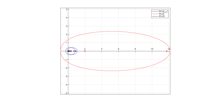
Figure 1: Numerical ranges of the tensors $\mathcal{A}$, $\mathcal{A}^{\dagger}$, and $\mathcal{A}_{\mathcal{M},\mathcal{N}}^{{\dagger}}$

7 Conclusions

In this article, we have introduced the notion of the WSVD and derived the formula for computing the weighted Moore-Penrose inverse of an arbitrary-order tensor using the WSVD. After that, we have defined the notions of weighted normal tensor and weighted tensor norm. Further, we have established several properties that examine some relationship between a tensor’s numerical range and its weighted Moore-Penrose inverse. An upper bound for the product of the numerical radii of a weighted shift matrix and its weighted Moore-Penrose inverse with diagonal weights has been established. An equality between the numerical ranges of the weighted Moore-Penrose inverse and the weighted conjugate transpose of a special tensor has been given. Our work on numerical ranges and numerical radii will also be beneficial in finding the iterative solution to tensor equations. These theories add new contributions to the theory of tensors and will be crucial for future research on tensors.

Conflict of Interest

The authors declare that there is no conflict of interest.

Data Availability Statement

Data sharing is not applicable to this article as no new data is analyzed in this study.

References

• [1] Axelsson, O.; Lu, H.; Polman, B., On the numerical radius of matrices and its application to iterative solution methods, Linear Multilinear Algebra, 37 (1994) 225-238.
• [2] Behera, R.; Maji, S.; Mohapatra, R. N., Weighted Moore-Penrose inverses of arbitrary-order tensors, Comput. Appl. Math., 39 (2020) Article number: 284.
• [3] Bonsall, F. F.; Duncan, J., Numerical Ranges I, Cambridge University Press, Cambridge, 1971.
• [4] Bonsall, F. F.; Duncan, J., Numerical Ranges II, Cambridge University Press, Cambridge, 1973.
• [5] Brazell, M.; Li, N.; Navasca, C.; Tamon, C., Solving multilinear systems via tensor inversion, SIAM J. Matrix Anal. Appl., 34 (2013) 542-570.
• [6] Cheng, S. H.; Higham, N. J., The nearest definite pair for the Hermitian generalized eigenvalue problem, Linear Algebra Appl., 302/303 (1999) 63-76.
• [7] Chien, M. T., On the numerical range of tridiagonal operators, Linear Algebra Appl., 246 (1996) 203-214.
• [8] Chien, M. T., Numerical range of Moore-Penrose inverse matrices, Mathematics, 8 (2020) Article number: 830.
• [9] Eiermann, M., Field of values and iterative methods, Linear Algebra Appl., 180 (1993) 167-197.
• [10] Einstein, A., The foundation of the general theory of relativity. In: Kox AJ, Klein MJ, Schulmann R, editors. The collected papers of Albert Einstein 6. Princeton (NJ): Princeton University Press; 2007.p. 146-200.
• [11] Fiedler, M., Numerical range of matrices and Levinger’s theorem, Linear Algebra Appl., 220 (1995) 171-180.
• [12] Goldberg, M.; Tadmor, E., On the numerical radius and its applications, Linear Algebra Appl., 42 (1982) 263-284.
• [13] Halmos, P. R., A Hilbert Space Problem Book, Von Nostrand, New York, 1967.
• [14] Horn, R. A.; Johnson, C. R., Topics in Matrix Analysis, Cambridge University Press, Cambridge, 1991.
• [15] Huang, B.; Li, W., Numerical subspace algorithms for solving the tensor equations involving Einstein product, Numer. Linear Algebra Appl., 28 (2021) Article number: e2351.
• [16] Ji, J.; Wei, Y., Weighted Moore-Penrose inverses and fundamental theorem of even-order tensors with Einstein product, Front. Math. China, 12 (2017) 1319-1337.
• [17] Jozi, M.; Karimi, S., A weighted singular value decomposition for the discrete inverse problems, Numer. Linear Algebra Appl., 25 (2018) Article number: e2114.
• [18] Ke, R.; Li, W.; Ng, M. K., Numerical ranges of tensors, Linear Algebra Appl., 508 (2016) 100-132.
• [19] Kirkland, S.; Psarrakos, P.; Tsatsomeros, M., On the location of the spectrum of hypertournament matrices, Linear Algebra Appl., 323 (2001) 37-49.
• [20] Kyrchei, I., Weighted singular value decomposition and determinantal representations of the quaternion weighted Moore–Penrose inverse, Appl. Math. Comput., 309 (2017) 1-16.
• [21] Lai, W. M.; Rubin, D.; Krempl, E., Introduction to Continuum Mechanics, Butterworth-Heinemann, Oxford, 2009.
• [22] Liang, M.; Zheng, B., Further results on Moore–Penrose inverses of tensors with application to tensor nearness problems, Comput. Math. Appl., 77 (2019) 1282–1293.
• [23] Maroulas, J.; Psarrakos, P.; Tsatsomeros, M., Perron-Frobenius type results on the numerical range, Linear Algebra Appl., 348 (2002) 49-62.
• [24] Naeem, K.; Kim, B. H.; Yoon, D. J.; Kwon, I. B., Enhancing detection performance of the phase-sensitive OTDR based distributed vibration sensor using weighted singular value decomposition, Appl. Sci., 11 (2021) Article number: 1928.
• [25] Panigrahy, K.; Mishra, D., Extension of Moore–Penrose inverse of tensor via Einstein product, Linear Multilinear Algebra, 70 (2020) 750-773.
• [26] Panigrahy, K.; Mishra, D., On reverse-order law of tensors and its application to additive results on Moore–Penrose inverse, RACSAM, 114 (2020) Article Number: 184.
• [27] Panigrahy, K.; Behera, R.; Mishra, D., Reverse-order law for the Moore-Penrose inverses of tensors, Linear Multilinear Algebra, 68 (2020) 246-264.
• [28] Pakmanesh, M.; Afshin, H., Numerical ranges of even-order tensor, Banach J. Math. Anal., 15 (2021) Article number: 59.
• [29] Psarrakos, P.; Tsatsomeros, M., On the stability radius of matrix polynomials, Linear Multilinear Algebra, 50 (2002) 151-165.
• [30] Rout, N. C.; Panigrahy, K.; Mishra, D., A note on numerical ranges of tensors, Revision submitted to Linear Multilinear Algebra (2022) doi:10.1080/03081087.2022.2117771.
• [31] Ma, H.; Li, N.; Stanimirović, P. S.; Katsikis, V. N., Perturbation theory for Moore-Penrose inverse of tensor via Einstein product, Comput. Appl. Math., 38 (2019) Article number: 111.
• [32] Stanimirović, P. S.; Ćirić, M.; Katsikis, V. N.; Li, C.; Ma, H., Outer and (b,c) inverses of tensors, Linear Multilinear Algebra, 68 (2020) 940-971.
• [33] Sun, L.; Zheng, B.; Bu, C.; Wei, Y., Moore-Penrose inverse of tensors via Einstein product, Linear Multilinear Algebra, 64 (2016) 686-698.
• [34] Sergienko, I. V.; Galba, E. F., Weighted singular value decomposition of matrices with singular weights based on weighted orthogonal transformations, Cybern. Syst. Anal., 51 (2015) 514-528.
• [35] Van Loan, C. F., Generalizing the singular value decomposition, SIAM J. Numer. Anal., 13 (1976) 76-83.
• [36] Wang, D., Some topics on weighted Moore-Penrose inverse, weighted least squares and weighted regularized Tikhonov problems, Appl. Math. Comput., 157 (2004) 243-267.