Multi-modal Molecule Structure-text Model for Text-based Retrieval and Editing

Abstract

There is increasing adoption of artificial intelligence in drug discovery. However, existing studies use machine learning to mainly utilize the chemical structures of molecules but ignore the vast textual knowledge available in chemistry. Incorporating textual knowledge enables us to realize new drug design objectives, adapt to text-based instructions and predict complex biological activities. Here we present a multi-modal molecule structure-text model, MoleculeSTM, by jointly learning molecules’ chemical structures and textual descriptions via a contrastive learning strategy. To train MoleculeSTM, we construct a large multi-modal dataset, namely, PubChemSTM, with over 280,000 chemical structure-text pairs. To demonstrate the effectiveness and utility of MoleculeSTM, we design two challenging zero-shot tasks based on text instructions, including structure-text retrieval and molecule editing. MoleculeSTM has two main properties: open vocabulary and compositionality via natural language. In experiments, MoleculeSTM obtains the state-of-the-art generalization ability to novel biochemical concepts across various benchmarks.

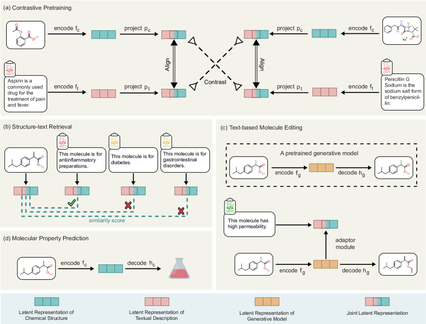
Figure 1: Pipeline of pretraining and downstream tasks. (a) MoleculeSTM pretraining with two branches, the chemical structure (green) and textual description (pink). (b) Structure-text retrieval downstream task. (c) Text-based molecule editing downstream task. (d) Molecular property prediction downstream task.

Recent progress in artificial intelligence (AI) promises to be transformative for drug discovery [1]. AI methods have been used to augment and accelerate current computational pipelines [2, 3, 4], including but not limited to virtual screening [96, 6], metabolic property prediction [7, 8, 90], and targeted chemical structure generation and editing [10, 67, 12, 78].

Existing machine learning (ML) methods mainly focus on modeling the chemical structure of molecules through one-dimensional descriptions [14], two-dimensional molecular graphs [7, 69, 8], or three-dimensional geometric structures [16, 17, 18]. They also use supervised signals, e.g., toxicity labels, quantum-mechanical properties, and binding affinity measurements. However, such a supervised setting requires expensive annotations on pre-determined label categories, impeding the application to unseen categories and tasks [19]. To overcome this issue, unsupervised pretraining on large-scale databases [20] has been proposed, with the main advantage being the ability to learn chemical structures without supervised annotation by reconstructing the masked topological [98] or geometric [22] substructures. Compared to the supervised setting, although such pretrained models [98, 22] have proven to be more effective in generalizing to various downstream tasks by fine-tuning on a few labeled examples, it is still an open challenge to generalize unseen categories and tasks without such labeled examples or fine-tuning (i.e., the so-called zero-shot setting [23] in ML). Additionally, existing molecule pretraining methods mostly incorporate only chemical structures, leaving the multi-modal representation less explored.

We have a vast amount of textual data that is human-understandable and easily accessible. This is now being harnessed in large-scale multi-modal models for images and videos [24, 25, 26, 27]. A natural language interface is an intuitive way to enable open vocabulary and description of tasks. Pretrained multi-modal models can generalize well to new categories and tasks, even in the zero-shot setting [24, 25, 26, 27]. They also enable agents to interactively learn to solve new tasks and explore new environments [28, 29]. We believe similar capabilities can also be obtained in molecular models by incorporating the vast textual knowledge available in the literature.

Previous work [30] has attempted to leverage the textual knowledge to learn the molecule representation. However, it only supports modeling with the 1D description (the simplified molecular-input line-entry system or SMILES) and learns the chemical structures and textual descriptions on a small-scale dataset (10K structure-text pairs). Furthermore, it unifies two modalities into a single language modeling framework and requires aligned data, i.e., chemical structure and text for each sample, for training. As a result, it cannot adopt existing powerful pretrained models, and the availability of aligned data is extremely limited.

Our approach: We design a multi-modal foundation model for molecular understanding that incorporates both molecular structural information and textual knowledge. We demonstrate zero-shot generalization to new drug design objectives using text-based instructions and to the prediction of new complex biological activities without the need for labeled examples or fine-tuning.

We propose MoleculeSTM, consisting of two branches: the chemical structure branch and the textual description branch, to handle the molecules’ internal structures and external domain knowledge, respectively. Such a disentangled design enables MoleculeSTM to be integrated with the powerful existing models trained on each modality separately, i.e., molecular structural models [67, 70] and scientific language models [64]. Given these pretrained models, MoleculeSTM bridges the two branches via a contrastive learning paradigm [70, 73].

To align such two branches with MoleculeSTM, we construct a structure-text dataset called PubChemSTM from PubChem [63], which is the largest multi-modal dataset to date in the community (28$\times$ larger than the existing dataset [30]). In PubChemSTM, each chemical structure is paired with a textual description, illustrating the chemical and physical properties or high-level bioactivities accordingly. Since MoleculeSTM is trained on a large-scale structure-text pair dataset and such textual data contains open-ended chemical information, it can be generalized to diverse downstream tasks in a zero-shot manner.

To demonstrate the advantages of introducing the language modality, we design two challenging downstream tasks: the structure-text retrieval task and text-based molecule editing task, and we apply the pretrained MoleculeSTM on them in a zero-shot manner. By studying these tasks, we summarize two main attributes of MoleculeSTM: the open vocabulary and compositionality. (1) Open vocabulary means our proposed MoleculeSTM is not limited to a fixed set of pre-defined molecule-related textual descriptions and can support exploring a wide range of biochemical concepts with the unbound vocabulary depicted by the natural language. In the drug discovery pipeline, such an attribute can be used for the text-based molecule editing in the lead optimization task and the novel disease-drug relation extraction in the drug re-purposing task. (2) Compositionality implies that we can express a complex concept by decomposing it into several simple concepts. This can be applied for the text-based multi-objective lead optimization task [84] where the goal is to generate molecules satisfying multiple properties simultaneously.

Empirically, MoleculeSTM reaches the best performance on six zero-shot retrieval tasks (up to 50% higher accuracy) and 20 zero-shot text-based editing tasks (up to 40% higher hit ratio) compared to the state-of-the-art methods. Furthermore, for molecular editing tasks, visual inspections reveal that MoleculeSTM can successfully detect critical structures implied in text descriptions. Additionally, we also explore whether MoleculeSTM can improve the performance on the standard molecular property prediction benchmark [90] via fine-tuning. Our results show that MoleculeSTM can achieve the best overall performance among nine baselines on eight property prediction tasks.

Results

Overview and Preliminaries

In this section, we first provide an overview of MoleculeSTM. Then, we introduce how to pretrain MoleculeSTM and apply the pretrained MoleculeSTM to three types of downstream tasks (Figure 1).

Overview. MoleculeSTM consists of two branches: the chemical structure branch and the textual description branch (${\bm{x}}_{c}$ and ${\bm{x}}_{t}$). The chemical structure branch illustrates the arrangement of atoms in a molecule. We consider two types of encoders $f_{c}$: Transformer [36] on the SMILES string and GNNs [7, 8, 69] on the 2D molecular graph. The textual description branch provides a high-level description of the molecule’s functionality, and we use the language model from a recent work [72] as the encoder $f_{t}$.

Pretraining. Within this design, MoleculeSTM aims to map the representations extracted from two branches to a joint space using two projectors ($p_{c}$ and $p_{t}$) via contrastive learning [70, 73]. The essential idea of contrastive learning is to reduce the representation distance between the chemical structure and textual description pairs of the same molecule and increase the representation distance between the pairs from different molecules. Specifically, we initialize these two branch encoders with the pretrained single-modal checkpoints [67, 70, 64] and then perform an end-to-end contrastive pretraining on collected dataset PubChemSTM. Specifically for PubChemSTM, it is constructed from PubChem [63]. We extract molecules with the textual description fields, leading to 281K chemical structure and text pairs. More details can be found in Supplementary A.1.

Two Principles for Downstream Task Design

We want to emphasize that for these downstream tasks, the language model in the pretrained MoleculeSTM reveals certain appealing attributes for molecule modeling and drug discovery. We summarize the two key points below.

Open vocabulary. Language is by nature open vocabulary and free form [38]. The large language model has proven its generalization ability in various art-related applications [24, 25, 26], and we find that it can also provide promising and insightful observations for drug discovery tasks. In this vein, our method is not limited to a fixed set of pre-defined molecule-related annotations but can support the exploration of novel biochemical concepts with unbound vocabulary. One example is the drug re-purposing. Suppose we have a textual description for a new disease or protein target functionality. In that case, we can obtain its similarity with all the existing drugs using MoleculeSTM and retrieve the drugs with the highest rankings, which can be adopted for the later stages, such as clinical trials. Another example is text-based lead optimization. We use natural language to depict an entirely new property, which can be reflected in the generated molecules after the optimization.

Compositionality. Another attribute is compositionality. In natural language, a complex concept can be expressed by decomposing it into simple concepts. This is crucial for certain domain-specific tasks, e.g., multi-objective lead optimization [84] where we need to generate molecules with multiple desired properties simultaneously. Existing solutions are either (1) learning one classifier for each desired property and doing filtering on a large candidate pool [10] or (2) optimizing a retrieval database to modify molecules to achieve the multi-objective goal [12]. The main limitation is that the success ratio highly depends on the availability of the labeled data for training the classifier or the retrieval database. While with the language model in MoleculeSTM, we provide an alternative solution. We first craft a natural text, called the text prompt, as the task description. The text prompt can be multi-objective and consists of the description for each property (e.g., “molecule is soluble in water and has high permeability”). With the pretrained joint space between chemical structures and textual descriptions, MoleculeSTM can transform the molecule property compositionality problem into the language compositionality problem, which is more tractable using the language model.

Downstream: Zero-shot Structure-text Retrieval

Experiments. For the zero-shot retrieval, we construct three datasets from DrugBank [76]. DrugBank is by far the most comprehensive database for drug-like molecules. Here we extract three fields in DrugBank: the description field, the pharmacodynamics field, and the anatomical therapeutic chemical (ATC) field. These fields illustrate the chemical properties and drug effects on the target organism. Then the retrieval task can be viewed as a $T$-choose-one multiple-choice problem, where $T$ is the number of choices. Specifically, we have two settings: (1) given chemical structure to retrieve the textual description and (2) given the textual description to retrieve the chemical structure. The retrieval accuracy is used as the evaluation metric.

Baselines. We first consider two baselines with the pretrained single-modal encoders [67, 70, 64]. (1) Frozen is that we take the pretrained encoders for the two branches and two randomly initialized projectors. (2) Similarity is that we take the similarity from a single branch only. For example, in the first setting, when given chemical structure, we retrieve the most similar chemical structure from PubChemSTM, then we take the corresponding paired text representation in PubChemSTM as the proxy representation. Based on this, we can calculate the similarity score between the proxy representation and $T$ requested text representations. (3) We further consider the third baseline, a pretrained language model for knowledgeable and versatile machine reading (KV-PLM) [30] on SMILES-text pairs.

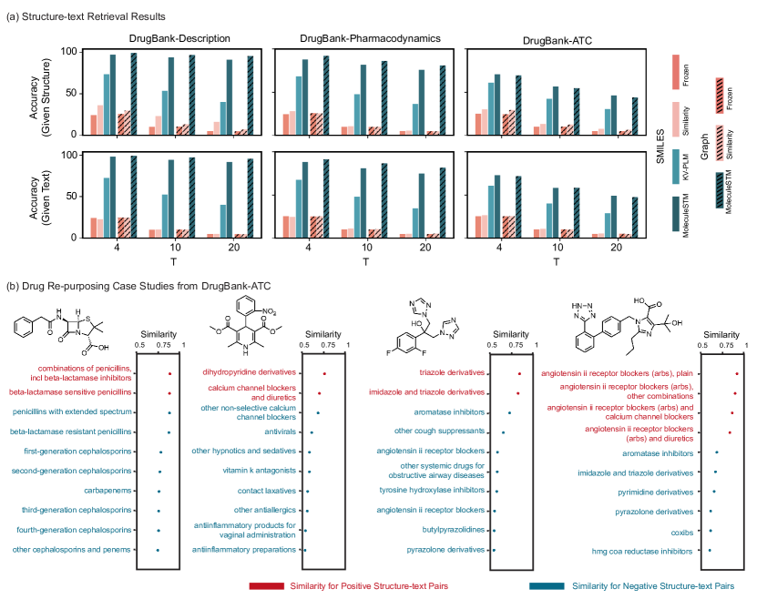
Figure 2: Results for zero-shot structure-text retrieval. (a) Accuracy for zero-shot structure-text retrieval on three DrugBank datasets. (b) Four case studies on DrugBank-ATC retrieval. HMG-CoA is $\beta$-Hydroxy $\beta$-methylglutaryl-CoA.

Results. The zero-shot retrieval results are shown in Figure 2 (a). First, we observe that all the algorithms’ accuracies are quite similar between the two settings. Then, as expected, we observe that the baseline Frozen performs no better than the random guess because of the randomly-initialized projectors. The Similarity baseline is better than the chance performance by a modest margin, verifying that the pretrained single-modality does learn semantic information but cannot generalize well between modalities. KV-PLM, on the other hand, learns semantically meaningful information from SMILES-text pairs, and thus, it achieves much higher accuracies on three datasets. For MoleculeSTM, the graph representation from GNNs has higher accuracy on Description and Pharmacodynamics than the SMILES representation from the transformer model; yet, both of them outperform all the other methods on three datasets and two settings by a large margin. For example, the accuracy improvements are around 50%, 40%, and 15% compared to the best baseline with $T=20$. Such large improvement gaps verify that MoleculeSTM can play a better role in understanding and bridging the two modalities of molecules.

Case study on drug re-purposing analysis. In Figure 2 (b), we further show four case studies on the retrieval quality of ATC. Specifically, given the molecule’s chemical structure, we take 10 (out of 600) most similar ATC labels. It is observed that MoleculeSTM can retrieve the ground-truth ATC labels with high rankings.

Downstream: Zero-shot Text-based Molecule Editing

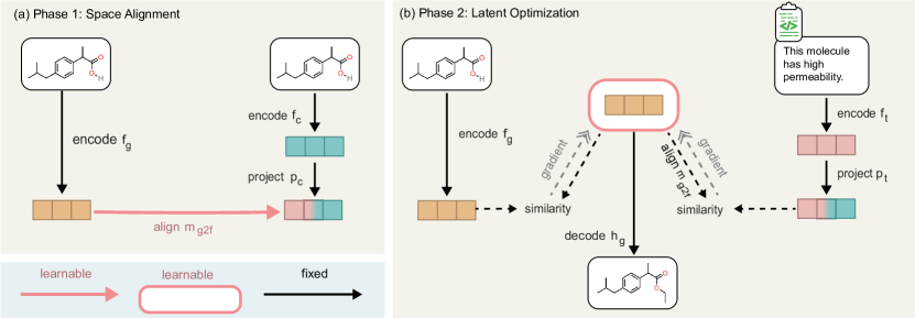
Figure 3: Pipelines for the zero-shot text-based molecule editing. (a) The space alignment step aligns the representation space of a pretrained molecule generation model and the representation space of MoleculeSTM. (b) The latent optimization step learns a latent representation that can be similar to both input molecules and textual descriptions.

Experiments. For molecule editing, we randomly sample 200 molecules from ZINC [20] and a text prompt as the inputs. Four categories of text prompts have been covered: (1) Single-objective editing is the text prompt using the single drug-related property for editing, such as “molecule with high solubility” and “molecule more like a drug”. (2) Multi-objective (compositionality) editing is the text prompt applying multiple properties simultaneously, such as “molecule with high solubility and high permeability”. (3) Binding-affinity-based editing is the text prompt for assay description, where each assay corresponds to one binding affinity task. A concrete example is ChEMBL 1613777 [79] with prompt as “This molecule is tested positive in an assay that are inhibitors and substrates of an enzyme protein. It uses molecular oxygen inserting one oxygen atom into a substrate, and reducing the second into a water molecule.”. The output molecules should possess higher binding affinity scores. (4) Drug relevance editing is the text prompt to make molecules structurally similar to certain common drugs, e.g., “this molecule looks like Penicillin”. We expect the output molecules to be more similar to the target drug than the input drug. For more detailed descriptions of the text prompts, please check Supplementary D. The evaluation is the satisfactory hit ratio, and it is a hit if the metric difference between output and input is over threshold $\Delta$. The $\Delta$ value is task-specific, and we consider two typical cases: $\Delta=0$ indicates a loose condition, and $\Delta>0$ is a strict condition with a larger positive influence. We provide the algorithm pipeline in Figure 3, and more details can be found in the Methods Section.

Baselines. We consider four baselines. The first three baselines [78] modify the representation of input molecules, followed by the decoding to the molecule space. Random is that we take a random noise as the perturbation to the representation of input molecules. PCA is that we take the eigenvectors as latent directions, where the eigenvectors are obtained after decomposing the latent representation of input molecules using principle component analysis (PCA). High Variance is that we take the latent representation dimension with the highest variance and apply the one-hot encoding on it as a semantic direction for editing. In addition, we also consider a baseline directly modifying the molecule space, the genetic search (GS). It is a variant of graph genetic algorithm [41], while the difference is that GS does a random search instead of a guided search by a reward function since no retrieval database is available in the zero-shot setting.

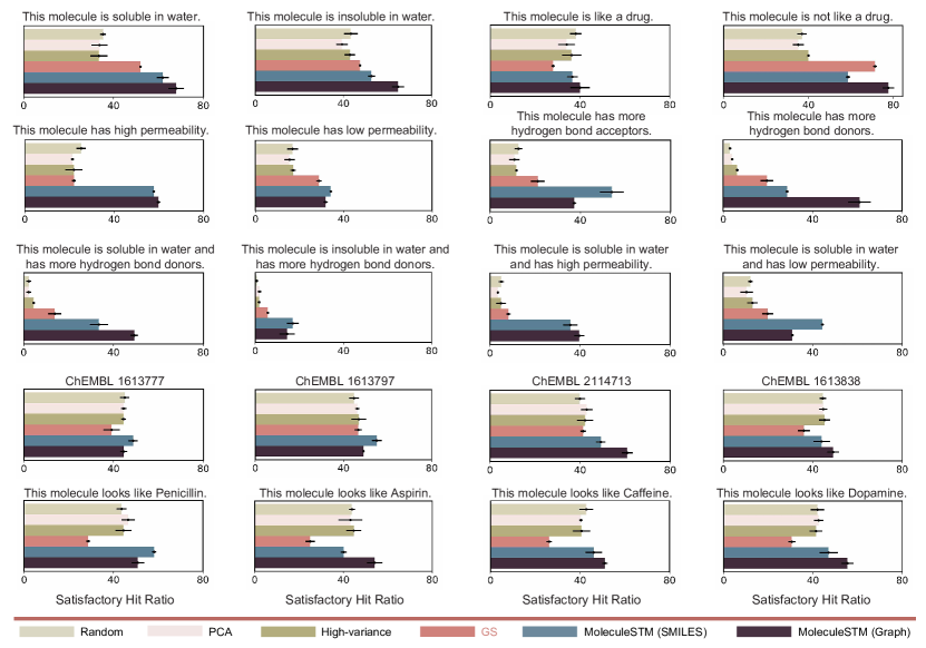
Figure 4: Visualization results for the zero-shot text-based molecule editing. Satisfactory hit ratios (%) of four types text-based editing tasks: eight single-objective, four multi-objective, four ChEMBL binding-affinity-based editing tasks (pretrained random forest as an evaluator, and detailed text prompts are in Supplementary D), and four drug relevance editing tasks. The satisfactory threshold ($\Delta$) is 0 for all visualized results. Each task runs for three random seeds, and the length of each error bar represents the standard deviation.

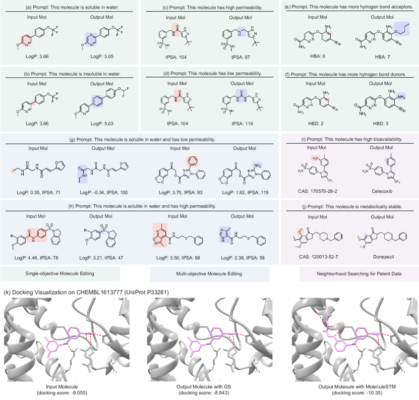
Figure 5: Visual analysis on text-based molecule editing. Case studies for solubility editing (a,b), permeability editing (c,d), acceptor and donor editing (e,f), solubility and permeability editing (g,h), and neighborhood searching for patent data (i,j). The pink and blue regions mark the functional groups before and after the editing, and we list the chemical abstracts service (CAS) registry number. (k) visualizes binding-affinity-based editing, and the dashed red lines mark the potential bindings.

Results. First, we provide the quantitative results for 20 editing tasks across four editing task types in Figure 4. The empirical results illustrate that the satisfactory hit ratios of MoleculeSTM are the best among all 20 tasks. It verifies that, for both SMILES and molecular graph encoders, MoleculeSTM enables a better semantic understanding of the natural language to explore output molecules with the desired properties. Next, we scrutinize the quality of output molecules in Figure 5 with detailed analysis as follows.

Visual analysis on single-objective molecule editing. We visually analyze the difference between input and output molecules using the single-objective property. Typical modifications are the addition, removal, and replacement of functional groups or cores of the molecules. For example, Figure 5 (a) and (b) show two different edits on the same molecule leading to opposite directions in solubility change depending on the text prompt. Replacement of pyridine to a pyrazine core improves the solubility, while insertion of a benzene linkage yields an insoluble molecule. In Figure 5 (c) and (d), changing an amide linkage to an alkyl amine and an urea results in higher and lower permeability of the edited molecules, respectively. Finally, Figure 5 (e) and (f) add a butyl ether and a primary amine to the exact position of the molecule, bringing more hydrogen bond acceptors and donors, respectively.

Visual analysis on multi-objective molecule editing. We further analyze the multi-objective (compositional) property editing. Water solubility improvement and permeability reduction are consistent when introducing polar groups to the molecule and removing lipophilic hydrocarbons, such as an amide or primary amine replacing a methyl or phenyl in Figure 5 (g). However, higher solubility and permeability are achievable if polar functionalities are removed or reduced in number together with hydrophobic components. For example, in Figure 5 (h), an amide and a benzene linkage are both removed in the left case, and a [1,2]oxazolo[5,4-b]pyridine substituent is replaced by a water-soluble imidazole with a smaller polar surface in the right case.

Case studies on neighborhood searching for patent drug molecules. In drug discovery, improvement of drug-like properties of lead molecules is crucial for finding drug candidates [84]. Herein we demonstrate two examples of generating approved drugs from their patented analogs by addressing their property deficiencies based on text prompts. Figure 5 (i) generates Celecoxib from its amino-substituted derivative [86], where the removal of the amino group yields a greater intestinal permeability of the molecule leading to higher bioavailability [87]. In Figure 5 (j), the trimethoxy benzene moiety, an electron-rich arene known to undergo oxidative phase I metabolisms [89], is replaced by a dimethoxy arene in Donepezil by calling for a metabolically stable molecule.

In summary, we conduct rich experiments on four types and 20 text-based molecule editing tasks, where the satisfactory hit ratios of MoleculeSTM are superior to baseline methods. Moreover, our editing results can match the expected outcomes based on chemistry domain knowledge. Both quantitative and qualitative results illustrate that MoleculeSTM can learn semantically meaningful information useful for domain applications, which encourages us to explore more challenging tasks with MoleculeSTM in the future.

Downstream: Molecular Property Prediction

method BBBP $\uparrow$ Tox21 $\uparrow$ ToxCast $\uparrow$ Sider $\uparrow$ ClinTox $\uparrow$ MUV $\uparrow$ HIV $\uparrow$ Bace $\uparrow$ Avg $\uparrow$ SMILES – (random initialized) 66.54$\pm$0.95 71.18$\pm$0.67 61.16$\pm$1.15 58.31$\pm$0.78 88.11$\pm$0.70 62.74$\pm$1.57 70.32$\pm$1.51 80.02$\pm$1.66 69.80 MegaMolBART 68.89$\pm$0.17 73.89$\pm$0.67 63.32$\pm$0.79 59.52$\pm$1.79 78.12$\pm$4.62 61.51$\pm$2.75 71.04$\pm$1.70 82.46$\pm$0.84 69.84 KV-PLM 70.50$\pm$0.54 72.12$\pm$1.02 55.03$\pm$1.65 59.83$\pm$0.56 89.17$\pm$2.73 54.63$\pm$4.81 65.40$\pm$1.69 78.50$\pm$2.73 68.15 MoleculeSTM 70.75$\pm$1.90 75.71$\pm$0.89 65.17$\pm$0.37 63.70$\pm$0.81 86.60$\pm$2.28 65.69$\pm$1.46 77.02$\pm$0.44 81.99$\pm$0.41 73.33 Graph – (random initialized) 63.90$\pm$2.25 75.06$\pm$0.24 64.64$\pm$0.76 56.63$\pm$2.26 79.86$\pm$7.23 70.43$\pm$1.83 76.23$\pm$0.80 73.14$\pm$5.28 69.99 AttrMask 67.79$\pm$2.60 75.00$\pm$0.20 63.57$\pm$0.81 58.05$\pm$1.17 75.44$\pm$8.75 73.76$\pm$1.22 75.44$\pm$0.45 80.28$\pm$0.04 71.17 ContextPred 63.13$\pm$3.48 74.29$\pm$0.23 61.58$\pm$0.50 60.26$\pm$0.77 80.34$\pm$3.79 71.36$\pm$1.44 70.67$\pm$3.56 78.75$\pm$0.35 70.05 InfoGraph 64.84$\pm$0.55 76.24$\pm$0.37 62.68$\pm$0.65 59.15$\pm$0.63 76.51$\pm$7.83 72.97$\pm$3.61 70.20$\pm$2.41 77.64$\pm$2.04 70.03 MolCLR 67.79$\pm$0.52 75.55$\pm$0.43 64.58$\pm$0.07 58.66$\pm$0.12 84.22$\pm$1.47 72.76$\pm$0.73 75.88$\pm$0.24 71.14$\pm$1.21 71.32 GraphMVP 68.11$\pm$1.36 77.06$\pm$0.35 65.11$\pm$0.27 60.64$\pm$0.13 84.46$\pm$3.10 74.38$\pm$2.00 77.74$\pm$2.51 80.48$\pm$2.68 73.50 MoleculeSTM 69.98$\pm$0.52 76.91$\pm$0.51 65.05$\pm$0.39 60.96$\pm$1.05 92.53$\pm$1.07 73.40$\pm$2.90 76.93$\pm$1.84 80.77$\pm$1.34 74.57

Table 1: Results on eight MoleculeNet binary classification tasks. Mean and standard deviation of test ROC-AUC on three random seeds are reported.

Experiments. One advantage for MoleculeSTM is that the pretrained chemical structure representation shares information with the external domain knowledge, and such implicit bias can be beneficial for the property prediction tasks. Similar to previous works on molecule pretraining [98, 70], we adopt the MoleculeNet benchmark [90]. It contains eight single-modal binary classification datasets to evaluate the expressiveness of the pretrained molecule representation methods. The evaluation metric is the area under the receiver operating characteristic curve (ROC-AUC) [45].

Baselines. We consider two types of chemical structures, the SMILES string and the molecular graph. For the SMILES string, we take three baselines: the randomly initialized models and two pretrained language models (MegaMolBART [67] and KV-PLM [30]). For the molecular graph, in addition to the random initialization, we consider five pretraining-based methods as baselines: AttrMasking [98], ContextPred [98], InfoGraph [46], MolCLR [99], and GraphMVP [8].

Results. As shown in Table 1, we first observe that pretraining-based methods improve the overall classification accuracy compared to the randomly-initialized ones. MoleculeSTM on the SMILES string has consistent improvements on six out of eight tasks compared to the three baselines. MoleculeSTM on the molecular graph performs the best on four out of eight tasks, while it performs comparably to the best baselines in other four tasks. In both cases, the overall performances (i.e., taking an average across all eight tasks) of MoleculeSTM are the best among all the methods.

Discussion

In this work, we have presented a multi-modal model, MoleculeSTM, to illustrate the effectiveness of incorporating textual descriptions for molecule representation learning. On two newly proposed zero-shot tasks and one standard property prediction benchmark, we confirmed consistently improved performance of MoleculeSTM compared to the existing methods. Additionally, we observed that MoleculeSTM can retrieve novel drug-target relations and successfully modify molecule substructures to gain the desired properties. These functionalities may accelerate various downstream drug discovery practices, such as re-purposing and multi-objective lead optimization. Furthermore, the outcomes of such downstream tasks have been found to be consistent with the feedback from chemistry experts, reflecting the domain knowledge exploration ability of MoleculeSTM.

One limitation of this work is data insufficiency. Although PubChemSTM is $28\times$ larger than the dataset used in existing works, it can be further improved and may require support from the entire community in the future. The second bottleneck of this work is the expressiveness of chemical structure models, including the SMILES encoder, the GNN encoder, and the SMILES-based molecule generative model. The development of more expressive architectures is perpendicular to this work and can be feasibly adapted to our multi-modal pretraining framework.

For future directions, we would like to extend MoleculeSTM from cheminformatics to bioinformatics tasks with richer textual information. This enables us to consider structure-based drug design problems such as protein-ligand binding and fragment design. Besides, the 3D geometric information has become more important for small molecules and polymers and can thus be merged into our foundation model. Last but not least, the tokenization of the textual description may require extra effort. Certain tasks possess rich terminologies (e.g., the ATC codes in DrugBank-ATC), and the overall performance is affected accordingly. Such fundamental problems should be handled carefully.

Methods

This section briefly describes certain modules in both pretraining and downstream tasks. Detailed specifications, such as dataset construction, model architectures, and hyperparameters, can be found in Supplementary A.

MoleculeSTM Pretraining

Dataset construction. For the structure-text pretraining, we consider the PubChem database [63] as the data source. PubChem includes 112M molecules, which is one of the largest public databases for molecules. The PubChem database has many fields, and previous work [30] uses the synonym field to match with an academic paper corpus [48], resulting in a dataset with 10K structure-text pairs. Meanwhile, the PubChem database has another field called “string” with more comprehensive and versatile molecule annotations. We utilize this field to construct a large-scale dataset called PubChemSTM, consisting of 250K molecules and 281K structure-text pairs.

In addition, even though PubChemSTM is the largest dataset with textual descriptions, its dataset size is comparatively small compared to the peers from other domains (e.g., 400M in the vision-language domain [24]). To mitigate such a data insufficiency issue, we adopt the pretrained models from existing checkpoints and then conduct the end-to-end pretraining, as will be discussed next.

Chemical structure branch $f_{c}$. This work considers two types of chemical structures: the SMILES string views the molecule as a sequence, and the 2D molecular graph takes the atoms and bonds as the nodes and edges, respectively. Then, based on the chemical structures, we apply a deep learning encoder $f_{c}$ to get a latent vector as molecule representation. Specifically, for the SMILES string, we take the encoder from MegaMolBART [67], which is pretrained on 500M molecules from ZINC database [68]. For the molecular graph, we take a pretrained graph isomorphism network (GIN) [69] using GraphMVP pretraining [70]. GraphMVP is doing a multi-view pretraining between the 2D topologies and 3D geometries on 250K conformations from GEOM dataset [71]. Thus, though we are not explicitly utilizing the 3D geometries, the state-of-the-art pretrained GIN models can implicitly encode such information.

Textual description branch $f_{t}$. The textual description branch provides a high-level description of the molecule’s functionality. We can view this branch as domain knowledge to strengthen the molecule representation. Such domain knowledge is in the form of natural language, and we use the BERT model [72] as the text encoder $f_{t}$. We further adapt the pretrained SciBERT [64], which was pretrained on the textual data from the chemical and biological domain.

Contrastive pretraining. For the MoleculeSTM pretraining, we adopt the contrastive learning strategy, e.g., EBM-NCE [70] and InfoNCE [73]. EBM-NCE and InfoNCE align the structure-text pairs for the same molecule and contrast the pairs for different molecules simultaneously. We consider the selection of contrastive pretraining methods as one important hyperparameter. The objectives for EBM-NCE and InfoNCE are

$$\mathcal{L}_{\text{EBM-NCE}} =-\frac{1}{2}\Big{(}\mathbb{E}_{{\bm{x}}_{c},{\bm{x}}_{t}}\big{[}\log\sigma(E({\bm{x}}_{c},{\bm{x}}_{t})\big{]}+\mathbb{E}_{{\bm{x}}_{c},{\bm{x}}_{t}^{\prime}}\big{[}\log(1-\sigma(E({\bm{x}}_{c},{\bm{x}}_{t}^{\prime}))\big{]}\Big{)}+\mathbb{E}_{{\bm{x}}_{c},{\bm{x}}_{t}}\big{[}\log\sigma(E({\bm{x}}_{c},{\bm{x}}_{t})\big{]}+\mathbb{E}_{{\bm{x}}_{c}^{\prime},{\bm{x}}_{t}}\big{[}\log(1-\sigma(E({\bm{x}}_{c}^{\prime},{\bm{x}}_{t}))\big{]}\Big{)},$$ (1)

$$\mathcal{L}_{\text{InfoNCE}} =-\frac{1}{2}\mathbb{E}_{{\bm{x}}_{c},{\bm{x}}_{t}}\Big{[}\log\frac{\exp(E({\bm{x}}_{c},{\bm{x}}_{t}))}{\exp(E({\bm{x}}_{c},{\bm{x}}_{t}))+\sum\limits_{{\bm{x}}_{t^{\prime}}}\exp(E({\bm{x}}_{c},{\bm{x}}_{t^{\prime}}))}+\log\frac{\exp(E({\bm{x}}_{c},{\bm{x}}_{t}))}{\exp(E({\bm{x}}_{c},{\bm{x}}_{t}))+\sum\limits_{{\bm{x}}_{c^{\prime}}}\exp(E({\bm{x}}_{c^{\prime}},{\bm{x}}_{t}))}\Big{]},$$

where $\sigma$ is the sigmoid activation function, ${\bm{x}}_{c}$ and ${\bm{x}}_{t}$ form the structure-text pair for each molecule, and ${\bm{x}}_{c^{\prime}}$ and ${\bm{x}}_{t^{\prime}}$ are the negative samples randomly sampled from the noise distribution, which we use the empirical data distribution. $E(\cdot)$ is the energy function with a flexible formulation, and we use the dot product on the jointly learned space, i.e., $E({\bm{x}}_{c},{\bm{x}}_{t})=\langle p_{c}\circ f_{c}({\bm{x}}_{c}),p_{t}\circ f_{t}({\bm{x}}_{t})\rangle$, where $\circ$ is the function composition.

Downstream: Zero-shot Structure-text Retrieval

Given a chemical structure and $T$ textual descriptions, the retrieval task is to select the textual description with the highest similarity to the chemical structure (or vice versa) based on a score calculated on the joint representation space. This is appealing for specific drug discovery tasks, such as drug re-purposing or indication expansion [30, 51]. We highlight that pretrained models are used for retrieval in the zero-shot setting, i.e., without model optimization for this retrieval task. Existing works [52] have witnessed the potential issue that utilizing the chemical structure alone is not sufficient, while MoleculeSTM enables a novel perspective by adopting the textual description with the utilization of the high-level functionality of molecules.

In such a zero-shot task setting, all the encoders ($f_{c},f_{t}$) and projectors ($p_{c},p_{t}$) are pretrained from MoleculeSTM, and stay frozen in this downstream task. An example of the retrieval task of setting (1) is

$$\small\text{Retrieval}({\bm{x}}_{c})=\arg\max_{\tilde{\bm{x}}_{t}}\Big{\{}\big{\langle}p_{c}\circ f_{c}({\bm{x}}_{c}),p_{t}\circ f_{t}(\tilde{\bm{x}}_{t})\big{\rangle}\Big{|}\tilde{\bm{x}}_{t}\in\text{T textual descriptions}\Big{\}}.$$ (2)

Downstream: Zero-shot Text-based Molecule Editing

The objective of the molecule editing task is to modify the chemical structure of molecules such as functional group change [53] and scaffold hopping [54, 55]. Traditional methods for molecule editing highly rely on domain experts and could be subjective or biased [56, 57]. ML methods have provided an alternative strategy to solve this issue. Given a fixed pretrained molecule generative model (encoder $f_{g}$ and decoder $h_{g}$), the ML editing methods learn a semantically meaningful direction on the latent representation (or latent code) space. The decoder $h_{g}$ then generates output molecules with the desired properties by moving along the direction. In MoleculeSTM, with the pretrained joint representation space, we can accomplish this task by injecting the textual description in a zero-shot manner. As shown in Figure 3 (a, b), we need two phases. The first phase is space alignment, where we train an adaptor module to align the representation space of the generative model to the joint representation space of MoleculeSTM. The second phase is latent optimization, where we directly learn the latent code using two similarity scores as the objective function. Finally, decoding the optimized latent code can lead to the output molecules. Notice that during this editing process, both the MoleculeSTM ($f_{c},p_{c},f_{t},p_{t}$) and a pretrained molecule generative model ($f_{g},h_{g}$) are frozen.

Phase 1: space alignment. In this phase, the goal is to learn an adaptor module to align the representation space of the generative model to the joint representation space of MoleculeSTM. Following the Gaussian distribution, the objective function is

$$\mathcal{L}=\|m_{g2f}\circ f_{g}({\bm{x}}_{c})-p_{c}\circ f_{c}({\bm{x}}_{c})\|^{2},$$ (3)

where $\circ$ is the function composition function, and $m_{g2f}$ is the adaptor module optimized to align the two latent spaces.

Phase 2: latent optimization. In this phase, given an input molecule ${\bm{x}}_{c,\text{in}}$ and a text prompt ${\bm{x}}_{t}$, the goal is to optimize a latent code $w$ directly. The optimal $w$ should be close to the representations of ${\bm{x}}_{c,\text{in}}$ and ${\bm{x}}_{t}$ simultaneously, as:

$$w=\operatorname*{arg\,min}_{w\in\mathcal{W}}\Big{(}-\mathcal{L}_{\text{cosine-sim}}\big{(}m_{g2f}(w),p_{t}\circ f_{t}({\bm{x}}_{t})\big{)}+\lambda\cdot\mathcal{L}_{l_{2}}\big{(}w,f_{g}({\bm{x}}_{c,\text{in}})\big{)}\Big{)},$$ (4)

where $\mathcal{W}$ is the latent code space, $\mathcal{L}_{\text{cosine-sim}}$ is the cosine-similarity, and $\mathcal{L}_{l_{2}}$ is the $l_{2}$ distance, and $\lambda$ is a coefficient to balance these two similarity terms. Finally, after we optimize the latent code $w$, we will do decoding using the decoder from the pretrained generative model to obtain the output molecule: ${\bm{x}}_{c,\text{out}}=h_{g}(w)$.

Evaluation. The evaluation metric is the satisfactory hit ratio. Suppose we have an input molecule ${\bm{x}}_{c,\text{in}}$ and a text prompt ${\bm{x}}_{t}$, the editing algorithm will generate an output molecule ${\bm{x}}_{c,\text{out}}$. Then we use the hit ratio to measure if the output molecule can satisfy the conditions as indicated in the text prompt.

$$\text{hit}({\bm{x}}_{c,\text{in}},{\bm{x}}_{t}) =\begin{cases}1,&\exists\lambda\,\text{, s.t. ${\bm{x}}_{c,\text{out}}$ = $h_{g}$ (w; $\lambda$) $\wedge$ satisfy }({\bm{x}}_{c,\text{in}},{\bm{x}}_{c,\text{out}},{\bm{x}}_{t})\\ 0,&\text{otherwise}\end{cases},\quad\quad\quad\text{hit}(t)=\frac{\sum_{i=1}^{N}\text{hit}({\bm{x}}_{c,\text{in}}^{i},{\bm{x}}_{t})}{N},$$ (5)

where $N$ is the total number of editing outputs, and $\text{satisfy}(\cdot)$ is the satisfaction condition. It is task-specific, and we list the five key points below. (1) For single-objective property-based editing, we use the logarithm of partition coefficient (LogP), quantitative estimate of drug-likeness (QED), and topological polar surface area (tPSA) as the proxies to measure the molecule solubility [58], drug likeness [59], and permeability [60], respectively. The count of hydrogen bond acceptors (HBA) and hydrogen bond donors (HBD) are calculated explicitly. It will be a successful hit once the measurement difference between the input molecule and output molecule is above a certain threshold $\Delta$. (2) For multiple-objective property-based editing, we feed in a text prompt describing multiple properties’ composition. The $\Delta$ is composed of the threshold on each individual property, and a successful hit needs to satisfy all the properties simultaneously. (3) For binding-affinity-based editing, we take the ground-truth data from ChEMBL to train a binary classifier and test if the output molecules have higher confidence than the input molecules, and $\Delta$ is fixed to 0. (4) For drug relevance editing, we use Tanimoto similarity to quantify the structural similarity [61]. It will be a hit if the similarity score between the output molecule and target drug is higher than the similarity between the input molecule and target drug by a threshold $\Delta$. (5) Besides, the choice of satisfactory threshold $\Delta$ is also task-specific, and the higher the values are, the stricter the satisfaction condition is. The details of the threshold values can be found in Supplementary D.

Downstream: Molecular Property Prediction

For modeling, we take the pretrained encoder $f_{c}$ and add a prediction head $h_{c}$ to predict a categorical-valued or scalar-valued molecular property such as binding affinity or toxicity. Both $f_{c}$ and $h_{c}$ are optimized to fit the target property, i.e., in a fine-tuning manner [98, 70].

Data Availability

All the datasets are provided at this Hugging Face link. Specifically for the release of PubChemSTM, we encountered a big challenge regarding the textual data license. As confirmed with the PubChem group, performing research on these data does not violate their license; however, PubChem does not possess the license for the textual data, which necessitates an extensive evaluation of the license for each of the 280 structure-text pairs in PubChemSTM. This has hindered the release of PubChemSTM. Nevertheless, we have (1) described the detailed preprocessing steps in Supplementary A.1, (2) provided the molecules with CID file in PubChemSTM and (3) have also provided the detailed preprocessing scripts. By utilizing these scripts, users can easily reconstruct the PubChemSTM dataset.

Code Availability

The source code can be found at this GitHub repository and Zenodo [62]. The scripts for pretraining and three downstream tasks are provided here. The checkpoints of the pretrained models are provided at this Hugging Face link. Beyond the methods described so far, to help users try our MoleculeSTM model, this release includes demos in notebooks. Furthermore, users can customize their own datasets by checking the datasets folder.

Author Contributions Statement

S.L., W.N., C.W., Z.Q., C.X., and A.A. conceived and designed the experiments. S.L. performed the experiments. S.L. and C.W. analyzed the data. S.L., C.W., and J.L. contributed analysis tools. S.L., W.N., C.W., J.L., Z.Q., L.L., J. T., C.X., and A.A. wrote the paper. J. T., C.X., and A.A. contributed equally to advising this project.

Competing Interests Statement

The authors declare no competing interests.

Supplementary Information

11_pretrain.tex

Appendix A Design Principles for Downstream Tasks

In this section, we discuss the key principles when designing downstream tasks.

Applicable Evaluation

One of the biggest differences between the foundation model in the vision-language domain and our MoleculeSTM can be reflected in the evaluation. Most of the vision and language tasks can be viewed as art problems, i.e., there does not exist a standard and exact solution that is applicable for evaluation. For instance, we can detect if the image is "a horse riding an astronaut" or "a panda making latte art" [75], but only visually not computationally, which prevents large-scale evaluation. This is not the case for drug discovery, because it is a scientific task, where the results (e.g., properties of the output molecules in the editing task) can be evaluated exactly, either in vitro or in silico. Following this, the physical experiments are usually expensive and long-lasting, so in this work, we want to focus on tasks that are computationally feasible for evaluation.

Fuzzy Matching

Specifically for the molecule editing task, the text prompts should follow the “fuzzy matching” criterion because there could exist multiple output molecules. This is in contradiction with "exact matching", where the output molecules are deterministic. For example, for the functional group change, we can feed in the prompts like "change the third nitrogen in the ring to oxygen". This prompt is very explicit with an exact solution, and there exist rule-based chemistry tools in handling this problem perfectly. Thus, text-based editing cannot show its benefits in this track. Instead, text-based editing can provide more benefits in the fuzzy matching setting by wandering around the semantically meaningful directions in the latent space. This also reflects the open vocabulary attribute of the language model that we have been focusing on.

Appendix B Downstream: Zero-shot Structure-text Retrieval

B.1 Dataset Construction

The DrugBank database [76] has many fields that can be interesting to explore drug discovery tasks. Here we extract three fields of each small molecule drug for the zero-shot retrieval task: the Description field, the Pharmacodynamics field, and the anatomical therapeutic chemical (ATC) field, as detailed below:

• DrugBank-Description. The Description field gives a high-level review of the drug’s chemical properties, history, and regulatory status.

• DrugBank-Pharmacodynamics. This illustrates how the drug modifies or affects the organism it is being used in. This field may include effects in the body that are desired and undesired (also known as the side effects).

• DrugBank-ATC. Anatomical therapeutic chemical (ATC) is a classification system that categorizes the molecule into different groups according to the organ or system on which they act and their therapeutic, pharmacological, and chemical properties.

We list the key steps in dataset construction as follows:

1. We download the full DrugBank database (in XML format) and small chemical structure files (in SDF format) from the website.

2. We parse the XML file, and extract the data with three fields: Description, Pharmacodynamics, and ATC.

3. We do the mapping from the extracted files to chemical structures in SDF files. For DrugBank-Description and DrugBank-Pharmacodynamics datasets, we exclude the molecules that have shown up in PubChemSTM, filtered with the canonical SMILES. Meanwhile, for DrugBank-ATC, we exclude the molecules satisfying the following two criteria simultaneously:

   • Chemical structure filtering If the molecule with the same canonical SMILES has shown up in the PubChemSTM;

   • Textual data filtering We first need to define a similarity between two textual data as in Equation 6, where $\text{text}_{\text{DrugBank}}$ and $\text{text}_{\text{PubChemSTM}}$ are the textual data for the same molecule from DrugBank and PubChemSTM, respectively, len() is the length of textual data, and Levenshtein() is the Levenshtein distance between two textual data. Thus, the second condition is: if the similarity between the DrugBank text and the PubChemSTM text is above a certain threshold (e.g., 0.6).

   Another detail is that, for DrugBank-ATC, there exist multiple ATC fields ($\text{text}_{\text{DrugBank}}$) for each small molecule. In PubChemSTM, there also exist multiple textual descriptions ($\text{text}_{\text{PubChemSTM}}$) for each molecule. Thus during the textual data filtering step, for each shared molecule between DrugBank and PubChemSTM, we calculate the similarity for all the $\text{text}_{\text{DrugBank}}$-$\text{text}_{\text{PubChemSTM}}$ pairs, and exclude the molecule if there exists one pair with similarity above the threshold 0.6.

4. Some basic dataset statistics can be found in Table 2. Notice that ATC has many levels, and we are using level 5 for retrieval in this work.

$$\small\text{sim}\big{(}\text{text}_{\text{DrugBank}},\text{text}_{\text{PubChemSTM}}\big{)}=1-\frac{\text{Levenshtein}\big{(}\text{text}_{\text{DrugBank}},\text{text}_{\text{PubChemSTM}}\big{)}}{\text{len}\big{(}\text{text}_{\text{DrugBank}}\big{)}}.$$ (6)

Table 2: Statistics on three fields in DrugBank. The filtering steps have been illustrated above.

Field # structure-text pairs molecule not in PubChemSTM # structure-text pairs molecule shared in PubChemSTM but text similarity below 0.6 total DrugBank-Description 1,154 – 1,154 DrugBank-Pharmacodynamics 1,005 – 1,005 DrugBank-ATC 1,507 1,500 3,007

B.2 Experiments

For experiments, we introduce three baselines in the main body. As a proof-of-concept, we carry out another baseline called Random. For Random, both encoders ($f_{c}$ and $f_{t}$) are randomly initialized. The zero-shot retrieval results on three datasets are shown in Tables 3, 4 and 5.

Table 3: Accuracy (%) of DrugBank-Description $T$-choose-one retrieval.

Given Chemical Structure Given Text T 4 10 20 4 10 20 SMILES Random 24.59 $\pm$ 1.14 10.12 $\pm$ 1.38 4.97 $\pm$ 0.42 24.54 $\pm$ 0.97 9.97 $\pm$ 0.81 5.09 $\pm$ 0.37 Frozen 25.07 $\pm$ 1.24 10.22 $\pm$ 1.19 5.12 $\pm$ 0.65 24.69 $\pm$ 1.87 10.20 $\pm$ 1.38 5.37 $\pm$ 1.15 Similarity 36.35 $\pm$ 0.59 23.22 $\pm$ 0.58 16.40 $\pm$ 0.59 22.74 $\pm$ 0.24 10.31 $\pm$ 0.24 5.34 $\pm$ 0.24 KV-PLM 73.80 $\pm$ 0.00 53.96 $\pm$ 0.29 40.07 $\pm$ 0.38 72.86 $\pm$ 0.00 52.55 $\pm$ 0.29 40.33 $\pm$ 0.00 MoleculeSTM 97.50 $\pm$ 0.46 94.18 $\pm$ 0.46 91.12 $\pm$ 0.46 98.21 $\pm$ 0.00 94.54 $\pm$ 0.37 91.97 $\pm$ 0.46 Graph Random 25.78 $\pm$ 1.43 10.71 $\pm$ 0.97 4.83 $\pm$ 1.00 24.98 $\pm$ 0.32 10.20 $\pm$ 0.40 4.80 $\pm$ 0.21 Frozen 24.01 $\pm$ 1.34 9.39 $\pm$ 0.92 4.85 $\pm$ 0.52 24.00 $\pm$ 1.66 9.91 $\pm$ 0.71 5.07 $\pm$ 0.75 Similarity 30.03 $\pm$ 0.38 13.63 $\pm$ 0.27 7.07 $\pm$ 0.10 24.81 $\pm$ 0.27 10.22 $\pm$ 0.24 4.74 $\pm$ 0.24 MoleculeSTM 99.15 $\pm$ 0.00 97.19 $\pm$ 0.00 95.66 $\pm$ 0.00 99.05 $\pm$ 0.37 97.50 $\pm$ 0.46 95.71 $\pm$ 0.46

Table 4: Accuracy (%) of DrugBank-Pharmacodynamics $T$-choose-one retrieval.

Given Chemical Structure Given Text T 4 10 20 4 10 20 SMILES Random 24.49 $\pm$ 0.68 9.73 $\pm$ 0.34 5.14 $\pm$ 0.57 25.61 $\pm$ 0.62 10.10 $\pm$ 0.91 5.07 $\pm$ 0.69 Frozen 25.47 $\pm$ 1.12 10.55 $\pm$ 0.75 5.48 $\pm$ 0.70 25.34 $\pm$ 0.41 9.86 $\pm$ 0.44 4.84 $\pm$ 0.26 Similarity 27.85 $\pm$ 0.03 10.75 $\pm$ 0.02 5.67 $\pm$ 0.01 24.58 $\pm$ 0.03 11.25 $\pm$ 0.03 5.29 $\pm$ 0.02 KV-PLM 68.38 $\pm$ 0.03 47.59 $\pm$ 0.03 36.54 $\pm$ 0.03 67.68 $\pm$ 0.03 48.00 $\pm$ 0.02 34.66 $\pm$ 0.02 MoleculeSTM 88.07 $\pm$ 0.01 81.70 $\pm$ 0.02 75.94 $\pm$ 0.02 88.46 $\pm$ 0.01 81.01 $\pm$ 0.02 74.64 $\pm$ 0.03 Graph Random 26.00 $\pm$ 0.37 9.65 $\pm$ 0.88 4.95 $\pm$ 0.36 25.11 $\pm$ 0.63 9.99 $\pm$ 0.62 4.82 $\pm$ 0.54 Frozen 25.49 $\pm$ 1.82 10.19 $\pm$ 1.47 4.74 $\pm$ 0.56 25.55 $\pm$ 0.45 10.15 $\pm$ 0.77 4.88 $\pm$ 0.55 Similarity 25.33 $\pm$ 0.27 9.89 $\pm$ 0.52 4.61 $\pm$ 0.08 25.28 $\pm$ 0.03 10.64 $\pm$ 0.02 5.47 $\pm$ 0.02 MoleculeSTM 92.14 $\pm$ 0.02 86.27 $\pm$ 0.02 81.08 $\pm$ 0.05 91.44 $\pm$ 0.02 86.76 $\pm$ 0.03 81.68 $\pm$ 0.03

Table 5: Accuracy (%) of molecule-ATC $T$-choose-one retrieval.

Given Chemical Structure Given Text T 4 10 20 4 10 20 SMILES Random 25.03 $\pm$ 0.33 9.83 $\pm$ 0.19 4.80 $\pm$ 0.22 25.44 $\pm$ 1.21 10.03 $\pm$ 0.94 5.11 $\pm$ 0.79 Frozen 25.05 $\pm$ 0.94 10.17 $\pm$ 0.63 4.99 $\pm$ 0.54 25.35 $\pm$ 0.78 10.32 $\pm$ 0.44 5.22 $\pm$ 0.34 Similarity 30.03 $\pm$ 0.00 13.35 $\pm$ 0.02 7.53 $\pm$ 0.02 26.74 $\pm$ 0.03 11.01 $\pm$ 0.00 5.62 $\pm$ 0.00 KV-PLM 60.94 $\pm$ 0.00 42.35 $\pm$ 0.00 30.32 $\pm$ 0.00 60.67 $\pm$ 0.00 40.19 $\pm$ 0.00 29.02 $\pm$ 0.00 MoleculeSTM 70.84 $\pm$ 0.07 56.75 $\pm$ 0.05 46.12 $\pm$ 0.07 73.07 $\pm$ 0.03 58.19 $\pm$ 0.03 48.97 $\pm$ 0.06 Graph Random 24.48 $\pm$ 0.66 9.97 $\pm$ 0.25 4.81 $\pm$ 0.34 25.48 $\pm$ 0.59 10.40 $\pm$ 0.37 5.38 $\pm$ 0.30 Frozen 24.19 $\pm$ 0.77 10.24 $\pm$ 0.71 4.87 $\pm$ 0.47 24.95 $\pm$ 1.52 10.07 $\pm$ 0.80 5.06 $\pm$ 0.36 Similarity 29.46 $\pm$ 0.00 12.34 $\pm$ 0.00 6.52 $\pm$ 0.00 25.78 $\pm$ 1.53 10.23 $\pm$ 0.70 5.06 $\pm$ 0.67 MoleculeSTM 69.33 $\pm$ 0.03 54.83 $\pm$ 0.04 44.13 $\pm$ 0.05 71.81 $\pm$ 0.05 58.34 $\pm$ 0.07 47.58 $\pm$ 0.05

B.3 Ablation Study: Fixed Pretrained Encoders

In the main body, we conduct pretraining by adopting pretrained single-modality checkpoints, i.e., the GraphMVP and MegaMolBART for $f_{c}$, and SciBERT for$f_{t}$. Then for MoleculeSTM pretraining, we use contrastive learning and update all the model parameters. Here we take an ablation study by only optimizing the projection layers to the joint space of the two branches ($p_{c},p_{t}$) while keeping the two encoders ($f_{c},f_{t}$) fixed. The results on the three datasets are shown in Tables 6, 7 and 8.

Table 6: Accuracy (%) of DrugBank-Description $T$-choose-one retrieval.

Given Chemical Structure Given Text T 4 10 20 4 10 20 SMILES Random 24.59 $\pm$ 1.14 10.12 $\pm$ 1.38 4.97 $\pm$ 0.42 24.54 $\pm$ 0.97 9.97 $\pm$ 0.81 5.09 $\pm$ 0.37 Frozen 25.07 $\pm$ 1.24 10.22 $\pm$ 1.19 5.12 $\pm$ 0.65 24.69 $\pm$ 1.87 10.20 $\pm$ 1.38 5.37 $\pm$ 1.15 Similarity 36.35 $\pm$ 0.59 23.22 $\pm$ 0.58 16.40 $\pm$ 0.59 22.74 $\pm$ 0.24 10.31 $\pm$ 0.24 5.34 $\pm$ 0.24 MoleculeSTM 47.64 $\pm$ 0.40 29.21 $\pm$ 0.47 19.69 $\pm$ 0.47 52.60 $\pm$ 0.46 32.24 $\pm$ 0.37 21.45 $\pm$ 0.37 Graph Random 25.78 $\pm$ 1.43 10.71 $\pm$ 0.97 4.83 $\pm$ 1.00 24.98 $\pm$ 0.32 10.20 $\pm$ 0.40 4.80 $\pm$ 0.21 Frozen 24.01 $\pm$ 1.34 9.39 $\pm$ 0.92 4.85 $\pm$ 0.52 24.00 $\pm$ 1.66 9.91 $\pm$ 0.71 5.07 $\pm$ 0.75 Similarity 30.03 $\pm$ 0.38 13.63 $\pm$ 0.27 7.07 $\pm$ 0.10 24.81 $\pm$ 0.27 10.22 $\pm$ 0.24 4.74 $\pm$ 0.24 MoleculeSTM 51.28 $\pm$ 0.00 31.99 $\pm$ 0.41 20.71 $\pm$ 0.47 55.27 $\pm$ 0.00 33.08 $\pm$ 0.00 21.77 $\pm$ 0.00

Table 7: Accuracy (%) of DrugBank-Pharmacodynamics $T$-choose-one retrieval.

Given Chemical Structure Given Text T 4 10 20 4 10 20 SMILES Random 24.49 $\pm$ 0.68 9.73 $\pm$ 0.34 5.14 $\pm$ 0.57 25.61 $\pm$ 0.62 10.10 $\pm$ 0.91 5.07 $\pm$ 0.69 Frozen 25.47 $\pm$ 1.12 10.55 $\pm$ 0.75 5.48 $\pm$ 0.70 25.34 $\pm$ 0.41 9.86 $\pm$ 0.44 4.84 $\pm$ 0.26 Similarity 27.85 $\pm$ 0.03 10.75 $\pm$ 0.02 5.67 $\pm$ 0.01 24.58 $\pm$ 0.03 11.25 $\pm$ 0.03 5.29 $\pm$ 0.02 MoleculeSTM 46.43 $\pm$ 0.00 27.42 $\pm$ 0.47 18.24 $\pm$ 0.47 52.53 $\pm$ 0.41 30.53 $\pm$ 0.00 19.98 $\pm$ 0.00 Graph Random 26.00 $\pm$ 0.37 9.65 $\pm$ 0.88 4.95 $\pm$ 0.36 25.11 $\pm$ 0.63 9.99 $\pm$ 0.62 4.82 $\pm$ 0.54 Frozen 25.49 $\pm$ 1.82 10.19 $\pm$ 1.47 4.74 $\pm$ 0.56 25.55 $\pm$ 0.45 10.15 $\pm$ 0.77 4.88 $\pm$ 0.55 Similarity 25.33 $\pm$ 0.27 9.89 $\pm$ 0.52 4.61 $\pm$ 0.08 25.28 $\pm$ 0.03 10.64 $\pm$ 0.02 5.47 $\pm$ 0.02 MoleculeSTM 46.29 $\pm$ 0.03 27.18 $\pm$ 0.02 17.73 $\pm$ 0.02 50.95 $\pm$ 0.04 31.65 $\pm$ 0.03 23.00 $\pm$ 0.03

Table 8: Accuracy (%) of DrugBank-ATC $T$-choose-one retrieval.

Given Chemical Structure Given Text T 4 10 20 4 10 20 SMILES Random 25.03 $\pm$ 0.33 9.83 $\pm$ 0.19 4.80 $\pm$ 0.22 25.44 $\pm$ 1.21 10.03 $\pm$ 0.94 5.11 $\pm$ 0.79 Frozen 25.05 $\pm$ 0.94 10.17 $\pm$ 0.63 4.99 $\pm$ 0.54 25.35 $\pm$ 0.78 10.32 $\pm$ 0.44 5.22 $\pm$ 0.34 Similarity 30.03 $\pm$ 0.00 13.35 $\pm$ 0.02 7.53 $\pm$ 0.02 26.74 $\pm$ 0.03 11.01 $\pm$ 0.00 5.62 $\pm$ 0.00 MoleculeSTM 43.41 $\pm$ 0.12 25.66 $\pm$ 0.06 15.69 $\pm$ 0.06 48.75 $\pm$ 0.11 29.44 $\pm$ 0.06 19.75 $\pm$ 0.03 Graph Random 24.48 $\pm$ 0.66 9.97 $\pm$ 0.25 4.81 $\pm$ 0.34 25.48 $\pm$ 0.59 10.40 $\pm$ 0.37 5.38 $\pm$ 0.30 Frozen 24.19 $\pm$ 0.77 10.24 $\pm$ 0.71 4.87 $\pm$ 0.47 24.95 $\pm$ 1.52 10.07 $\pm$ 0.80 5.06 $\pm$ 0.36 Similarity 29.46 $\pm$ 0.00 12.34 $\pm$ 0.00 6.52 $\pm$ 0.00 25.78 $\pm$ 1.53 10.23 $\pm$ 0.70 5.06 $\pm$ 0.67 MoleculeSTM 42.53 $\pm$ 0.07 24.34 $\pm$ 0.00 14.78 $\pm$ 0.03 48.91 $\pm$ 0.03 28.77 $\pm$ 0.07 19.28 $\pm$ 0.07

Appendix C Downstream: Zero-shot Text-based Molecule Editing

Molecule editing or controllable molecule generation refers to changing the structures of the molecules based on a given and pretrained molecule generative model. In this work, with the help of a large language model in MoleculeSTM, we are able to do the zero-shot text-based molecule editing. First, we would like to list two key challenges, comparing the editing task between the vision domain and molecule domain, as follows:

• Backbone generative model. For domains in vision, the image controllable generation can be quite feasible based on StyleGAN [77], a well-disentangled backbone model. However, it is nontrivial for deep molecule generative models. A recent work GraphCG [78] has explored the disentanglement property of the graph-based controllable molecule generation methods, and the conclusion is that, even though the backbone generative models are not perfectly disentangled, there still exist methods for controllable generation on highly structured data like molecular graphs or point clouds. Meanwhile, developing a novel disentangled molecule generative model is out of the scope of this work, since the editing solution by MoleculeSTM is model-agnostic, and can be easily generalized to future models.

• Evaluation. Image controllable generation is an art problem, i.e., it is subjective and can have multiple (or even infinitely many) answers. On the contrary, controllable molecule generation is a science problem, i.e., it is objective and has only a few answers. This has been discussed in Appendix A.

C.1 Experiment Set-up

Implementation Details

Because most of the modules are fixed, we only need to learn the adaptor module and the optimized latent code $w$. The two key hyperparameters are the learning rate {1e-2, 1e-3} and $\lambda\in\{1e1,1e0,1e-1,1e-2,1e-3\}$. As a fair comparison, for baselines, we take the form of $w=w_{\text{in}}+\alpha\cdot D$, where $D$ is obtained using random, PCA and variance and $\lambda\in\{1.0,1.5,2.0,2.5,3.0\}$. For GS, we repeat the random sampling five times of each input molecule.

Next, we will conduct the zero-shot text-based molecule editing on four types of editing tasks, as well as three case study, as discussed below:

• Single-objective molecule editing in Section C.2 (eight tasks).

• Multi-objective molecule editing in Section C.3 (six tasks).

• Binding-affinity-based molecule editing in Section C.4 (six tasks).

• Drug relevance editing in Section C.5 (four tasks).

• Neighborhood searching for patent drug molecules in Section C.6 (three case studies).

Due to the page limit, we only show four multi-objective and four binding-affinity-based editing tasks in the main body. Here we show more comprehensive results.

We want to mention that for single- and multi-objective editing, we randomly select 200 molecules from ZINC as the input molecules. None of these 200 input molecules appears in PubChemSTM. Furthermore, the random selection process ensures that the property distributions of these 200 molecules remain consistent with the entire dataset. Illustrated below (Figures 7 and 7) are three examples of molecular properties: LogP (measuring water solubility), tPSA (measuring permeability) and molecular weight.

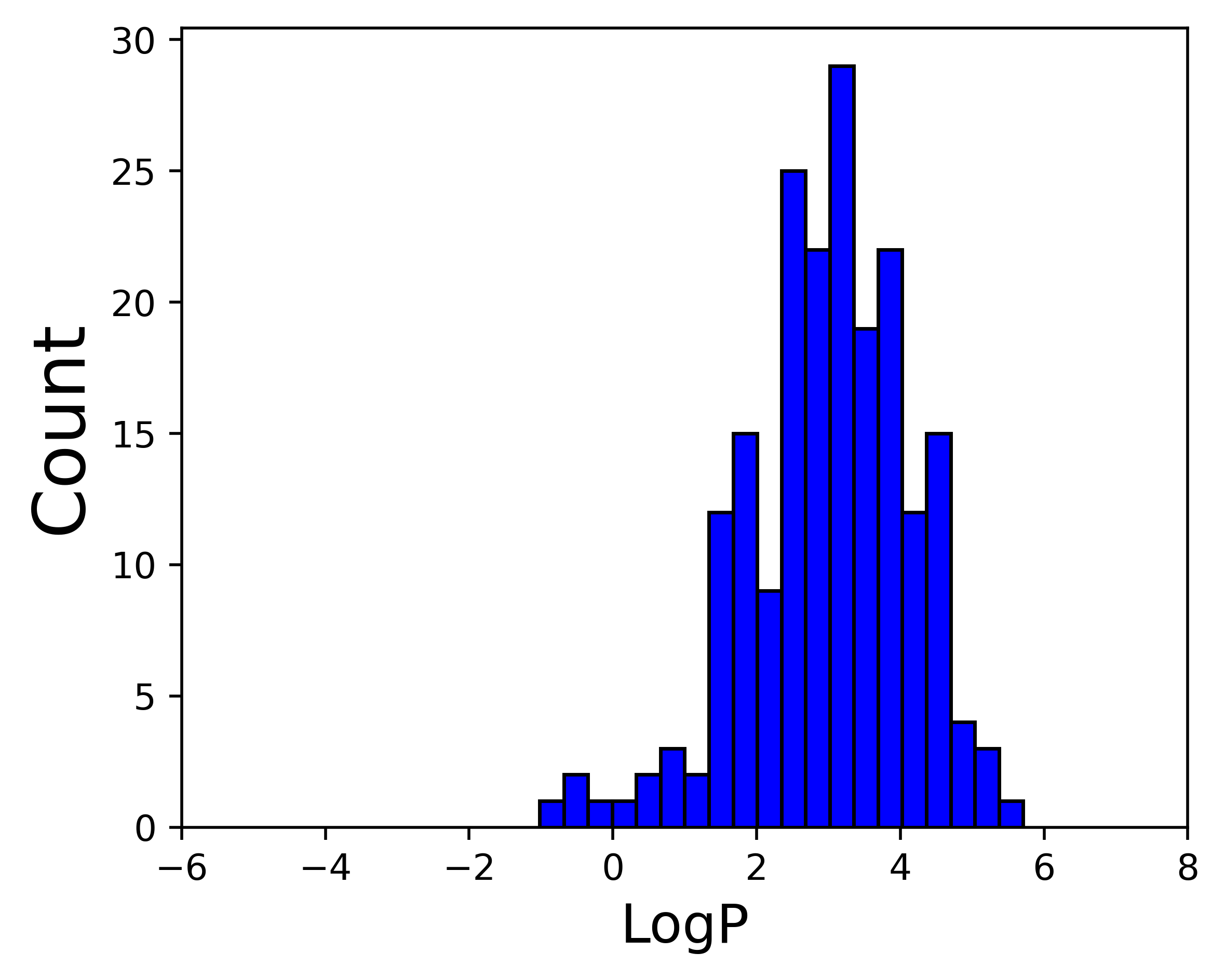
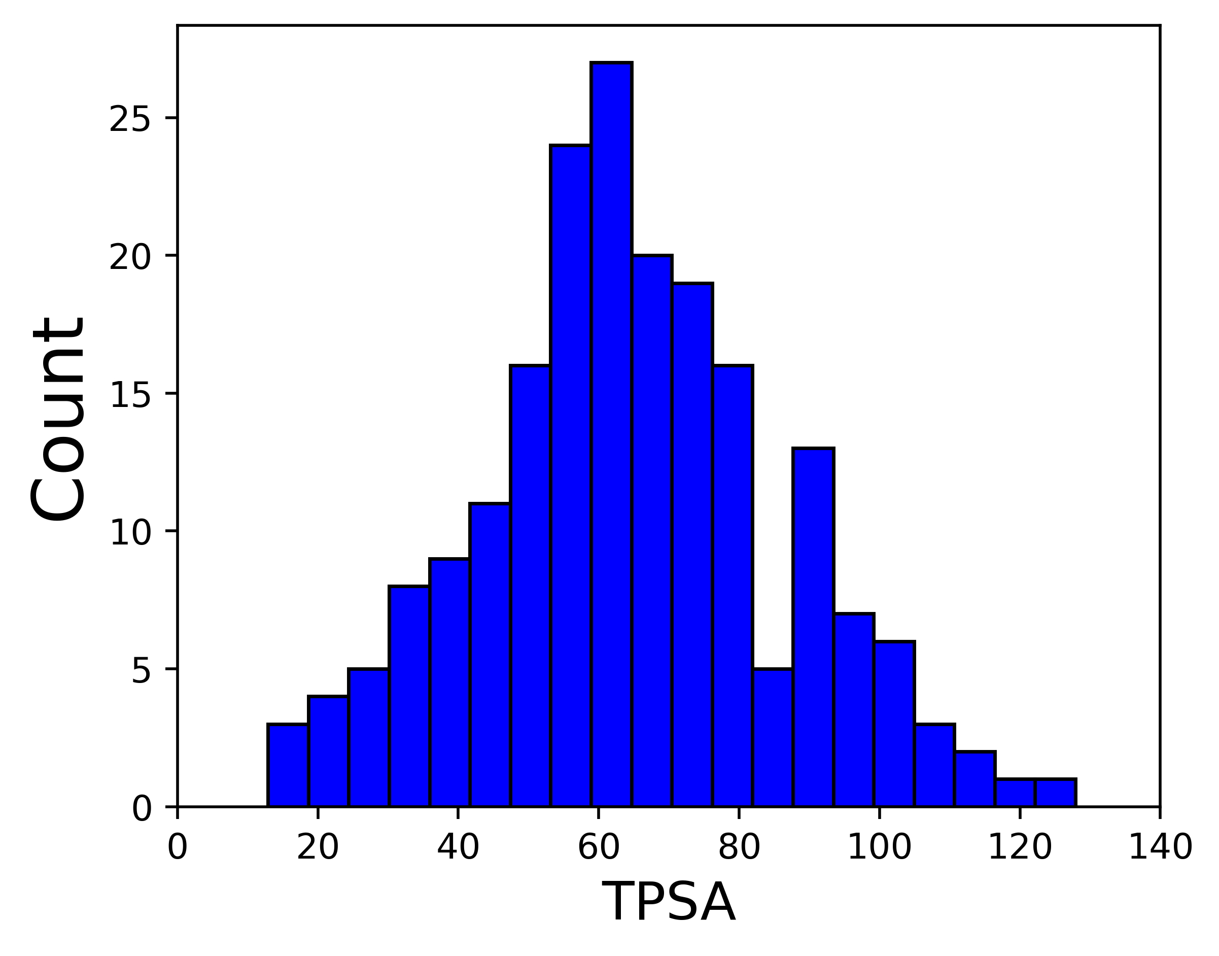
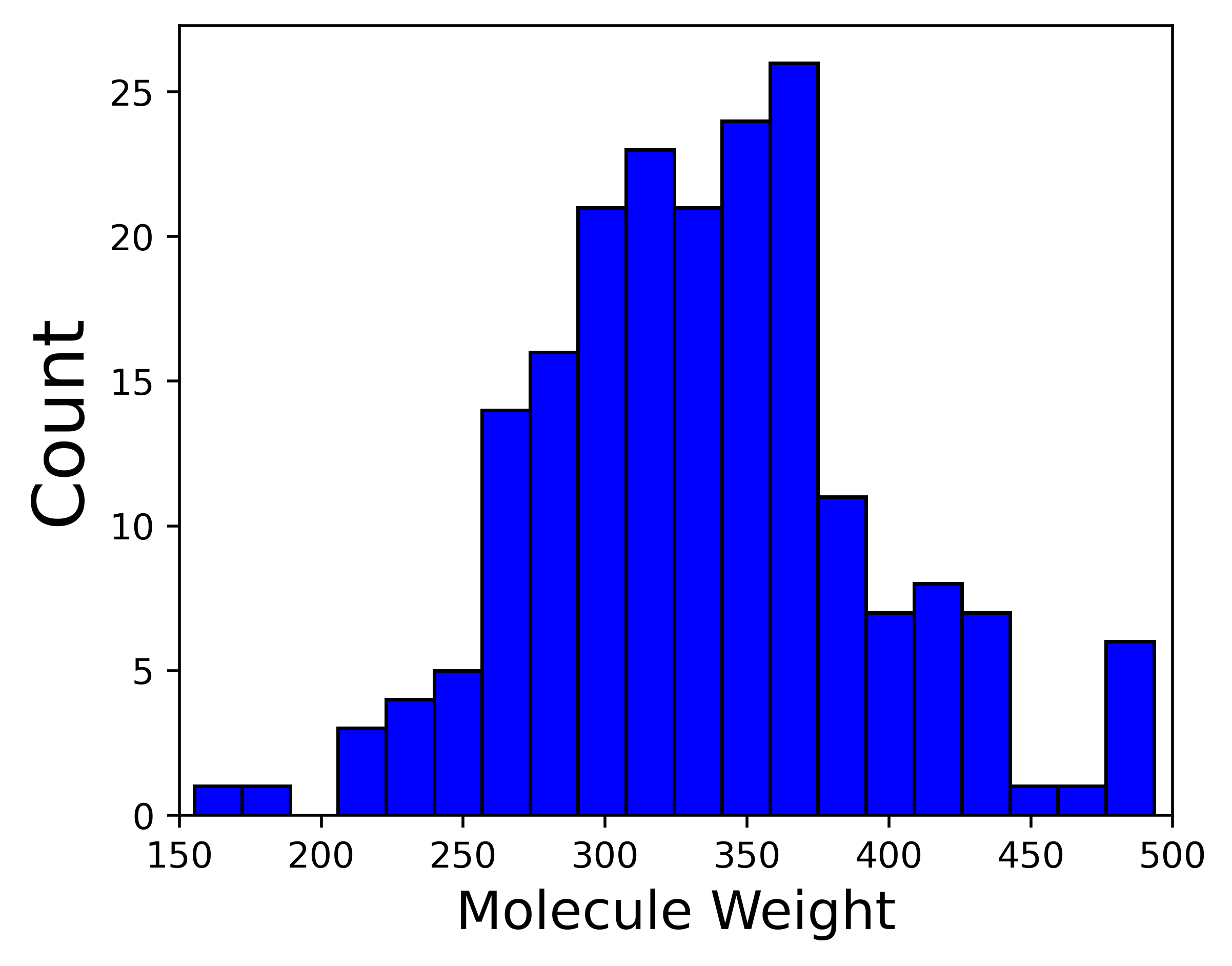
Figure 6: Three property distributions on 200 randomly sampled molecules for editing.

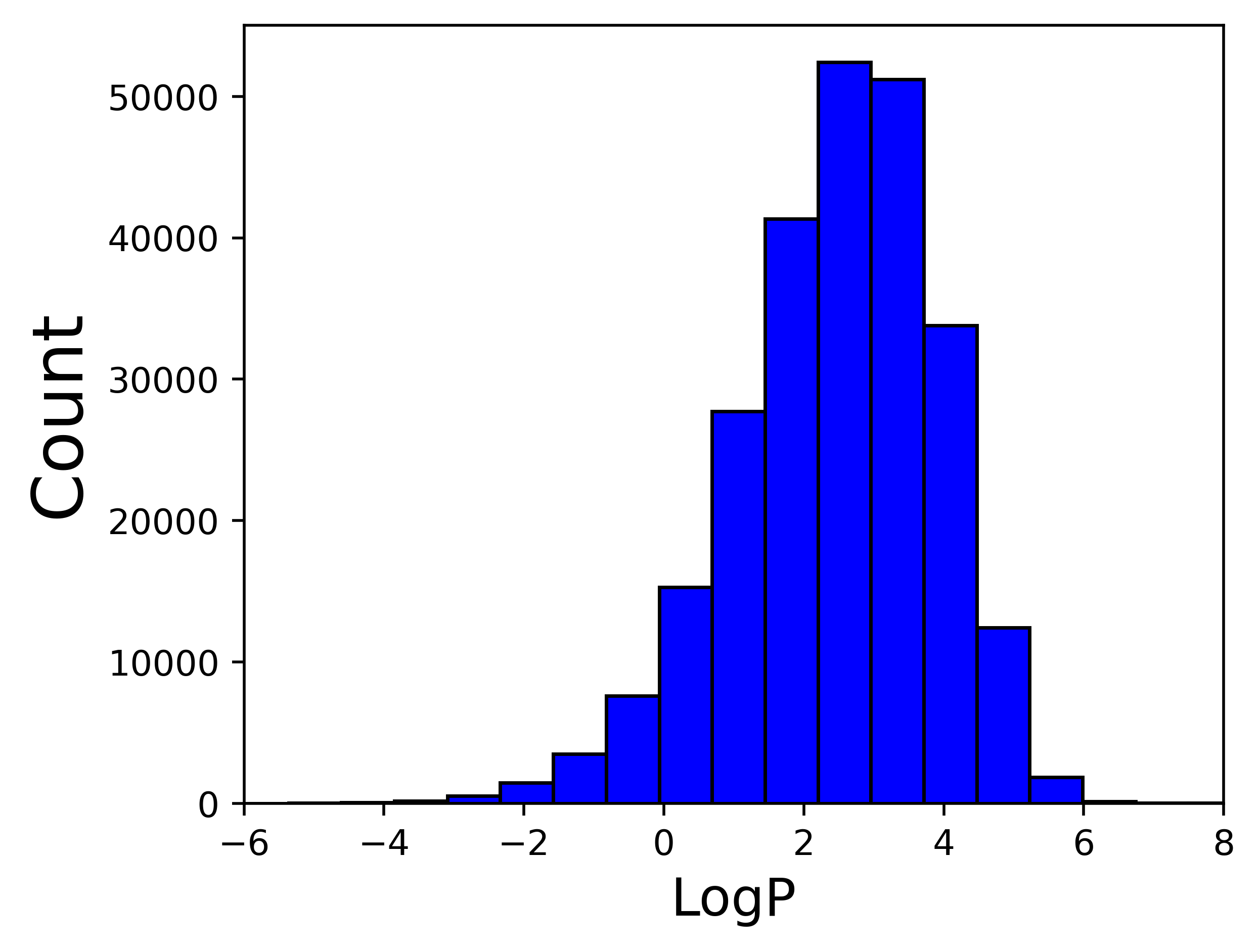
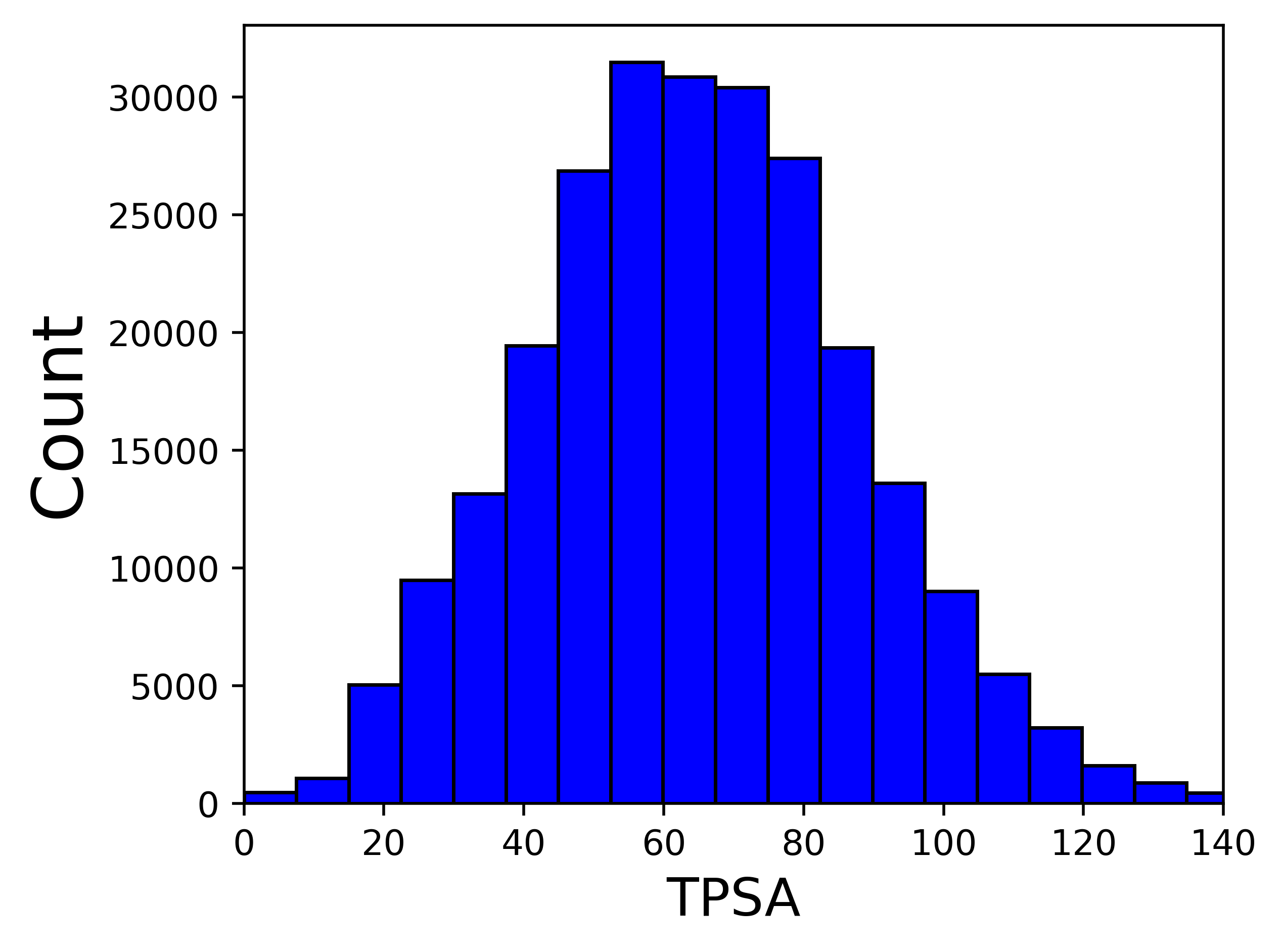
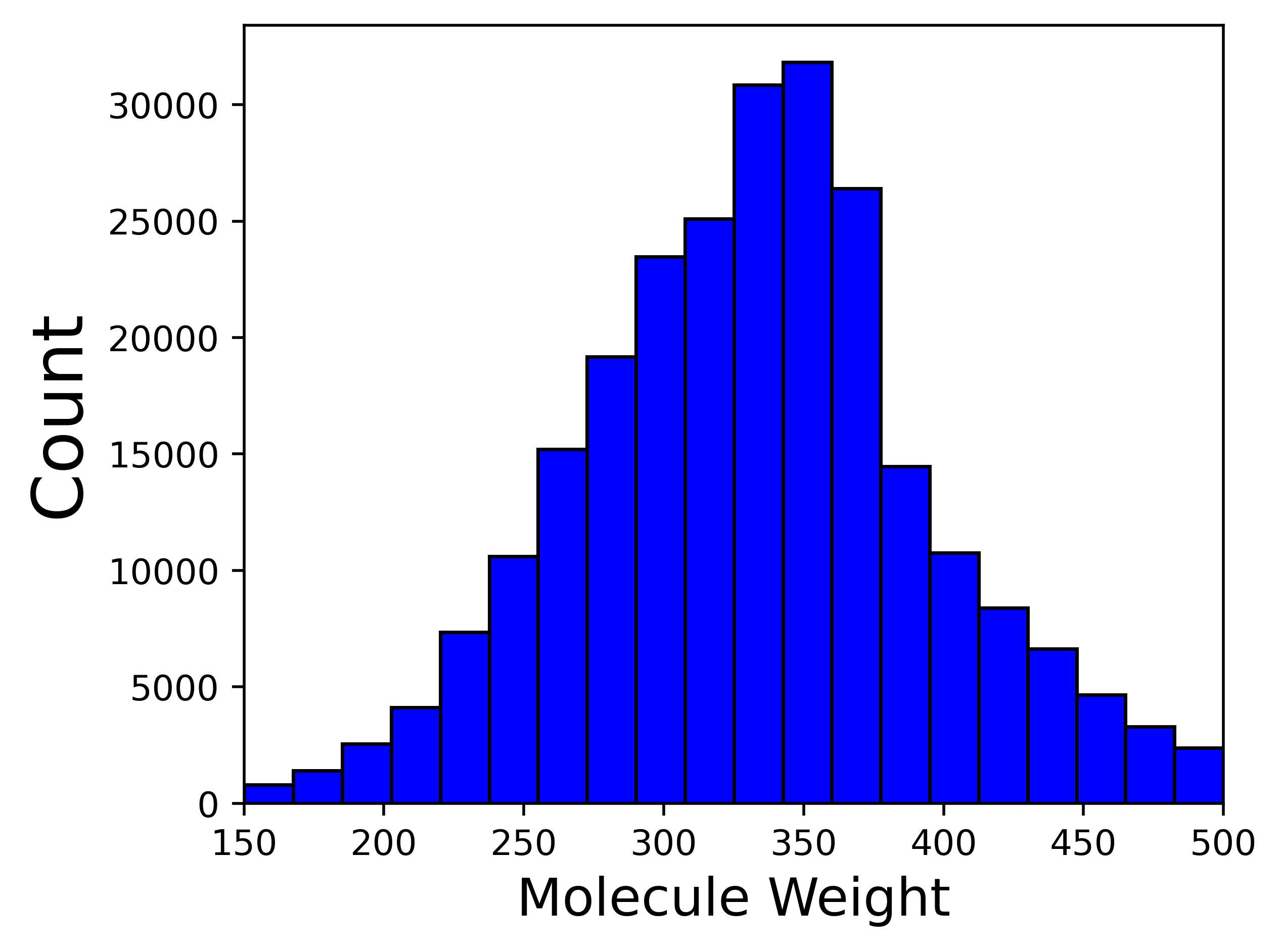
Figure 7: Three property distributions on 250K molecules from ZINC250K.

C.2 Single-objective Molecule Editing

We first consider eight single-objective properties for molecule editing. As shown in the Methods section, the definitions of the satisfaction function and threshold $\Delta$ are based on each task specifically, as:

• We use LogP to evaluate the solubility and insolubility. We take 0 and 0.5 as the different thresholds.

• We use QED to evaluate the drug-likeness. We take 0 and 0.1 as the different thresholds.

• We use tPSA to evaluate the high and low permeability. We take 0 and 10 as the different thresholds.

• For the hydrogen bond acceptor (HBA) and hydrogen bond donor (HBD), we can directly count them in the molecules, and we use 0 and 1 as the different thresholds.

For $\Delta$, it is the threshold that only difference above it can be viewed as a hit. So the larger $\Delta$ means a stricter editing criterion. Below we show both the quantitative and qualitative results on eight single-objective property molecule editing results.

Table 9: Results on eight single-objective molecule editing. The inputs are 200 molecules randomly sampled from ZINC, and the evaluation is the hit ratio of the property change. The latent optimization is text-based molecule editing with MoleculeSTM, with the SMILES string and the molecular graph, respectively.

baseline latent optimization $\Delta$ Random PCA High Variance GS-Mutate SMILES Graph This molecule is soluble in water. 0 35.33 $\pm$ 1.31 33.80 $\pm$ 3.63 33.52 $\pm$ 3.75 52.00 $\pm$ 0.41 61.87 $\pm$ 2.67 67.86 $\pm$ 3.46 0.5 11.04 $\pm$ 2.40 10.66 $\pm$ 3.24 10.86 $\pm$ 2.56 14.67 $\pm$ 0.62 49.02 $\pm$ 1.84 54.44 $\pm$ 3.99 This molecule is insoluble in water. 0 43.36 $\pm$ 3.06 39.36 $\pm$ 2.55 42.89 $\pm$ 2.36 47.50 $\pm$ 0.41 52.71 $\pm$ 1.67 64.79 $\pm$ 2.76 0.5 19.75 $\pm$ 1.56 15.12 $\pm$ 2.93 18.22 $\pm$ 0.33 12.50 $\pm$ 0.82 30.47 $\pm$ 3.26 47.09 $\pm$ 3.42 This molecule is like a drug. 0 38.06 $\pm$ 2.57 33.99 $\pm$ 3.72 36.20 $\pm$ 4.34 28.00 $\pm$ 0.71 36.52 $\pm$ 2.46 39.97 $\pm$ 4.32 0.1 5.27 $\pm$ 0.24 3.97 $\pm$ 0.10 4.44 $\pm$ 0.58 6.33 $\pm$ 2.09 8.81 $\pm$ 0.82 14.06 $\pm$ 3.18 This molecule is not like a drug. 0 36.96 $\pm$ 2.25 35.17 $\pm$ 2.61 39.99 $\pm$ 0.57 71.33 $\pm$ 0.85 58.59 $\pm$ 1.01 77.62 $\pm$ 2.80 0.1 6.16 $\pm$ 1.87 5.26 $\pm$ 0.95 7.56 $\pm$ 0.29 27.67 $\pm$ 3.79 37.56 $\pm$ 1.76 54.22 $\pm$ 3.12 This molecule has high permeability. 0 25.23 $\pm$ 2.13 21.36 $\pm$ 0.79 21.98 $\pm$ 3.77 22.00 $\pm$ 0.82 57.74 $\pm$ 0.60 59.84 $\pm$ 0.78 10 17.41 $\pm$ 1.43 14.52 $\pm$ 0.80 14.66 $\pm$ 2.13 6.17 $\pm$ 0.62 47.51 $\pm$ 1.88 50.42 $\pm$ 2.73 This molecule has low permeability. 0 16.79 $\pm$ 2.54 15.48 $\pm$ 2.40 17.10 $\pm$ 1.14 28.83 $\pm$ 1.25 34.13 $\pm$ 0.59 31.76 $\pm$ 0.97 10 11.02 $\pm$ 0.71 10.62 $\pm$ 1.86 12.01 $\pm$ 1.01 15.17 $\pm$ 1.03 26.48 $\pm$ 0.97 19.76 $\pm$ 1.31 This molecule has more hydrogen bond acceptors. 0 12.64 $\pm$ 1.64 10.85 $\pm$ 2.29 11.78 $\pm$ 0.15 21.17 $\pm$ 3.09 54.01 $\pm$ 5.26 37.35 $\pm$ 0.79 1 0.69 $\pm$ 0.01 0.90 $\pm$ 0.84 0.67 $\pm$ 0.01 1.83 $\pm$ 0.47 27.33 $\pm$ 2.62 16.13 $\pm$ 2.87 This molecule has more hydrogen bond donors. 0 2.97 $\pm$ 0.61 3.97 $\pm$ 0.55 6.23 $\pm$ 0.66 19.50 $\pm$ 2.86 28.55 $\pm$ 0.76 60.97 $\pm$ 5.09 1 0.00 $\pm$ 0.00 0.00 $\pm$ 0.00 0.00 $\pm$ 0.00 1.33 $\pm$ 0.24 7.69 $\pm$ 0.56 32.35 $\pm$ 2.57

Table 10: Visualization of text-based editing on solubility, measured by the logarithm of the octanol-water partition coefficient (LogP) of the molecules. Generally, molecules with smaller LogP are more soluble in water. For generating molecules soluble in water, we can add polar components (e.g., oxygens and nitrogens), remove hydrophobic moieties (e.g., benzene and cyclohexane), or replace hydrophobic groups with polar functionalities in the input molecule. For generating molecules insoluble in water, we can make opposite modifications to the input molecule. The pink and blue regions highlight the modified structure in the input and output molecules, respectively.

Text Prompt: This molecule is soluble in water. Input Molecule Output Molecule Input Molecule Output Molecule Input Molecule Output Molecule LogP: 3.66 LogP: 3.05 LogP: 3.72 LogP: 2.56 LogP: 4.25 LogP: 2.76 Text Prompt: This molecule is insoluble in water. Input Molecule Output Molecule Input Molecule Output Molecule Input Molecule Output Molecule LogP: 3.66 LogP: 5.03 LogP: -0.36 LogP: 0.72 LogP: 2.37 LogP: 4.41

Table 11: Visualization of text-based editing on permeability, measured by the topological polar surface area (tPSA) of the molecules. Generally, molecules with smaller tPSA are more permeable. For generating molecules with high permeability, we can remove functional groups or heterocycles with high polarity from the input molecule, such as amides, sulfonamides, ureas, nitro groups, and nitrogen-containing arenes. For generating molecules with low permeability, we can make opposite modifications to the input molecule. The pink and blue regions highlight the modified structure in the input and output molecules, respectively.

Text Prompt: This molecule has high permeability. Input Molecule Output Molecule Input Molecule Output Molecule Input Molecule Output Molecule tPSA: 104 tPSA: 87 tPSA: 96 tPSA: 68 tPSA: 76 tPSA: 20 Text Prompt: This molecule has low permeability. Input Molecule Output Molecule Input Molecule Output Molecule Input Molecule Output Molecule tPSA: 104 tPSA: 116 tPSA: 42 tPSA: 67 tPSA: 20 tPSA: 46

Table 12: Visualization of text-based editing on hydrogen bond acceptors (HBA) and hydrogen bond donors (HBD). For generating molecules with more HBA, we can add heteroatoms to the input molecule such as oxygen, nitrogen, and sulfur, or replace existing groups with heteroatom-containing structural motifs. For generating molecules with more HBD, we can add heteroatoms that bear attached hydrogens, such as functional groups like amines, and heterocycles like pyrroles. The pink and blue regions highlight the modified structure in the input and output molecules, respectively.

Text Prompt: This molecule has more hydrogen bond acceptors. Input Molecule Output Molecule Input Molecule Output Molecule Input Molecule Output Molecule HBA: 6 HBA: 7 HBA: 5 HBA: 6 HBA: 3 HBA: 5 Text Prompt: This molecule has more hydrogen bond donors. Input Molecule Output Molecule Input Molecule Output Molecule Input Molecule Output Molecule HBD: 2 HBD: 3 HBD: 2 HBD: 3 HBD: 1 HBD: 2

C.3 Multi-objective Molecule Editing

We then consider six multi-objective properties for molecule editing. As shown in the Methods section, the definitions of the satisfaction function and threshold $\Delta$ are based on each task specifically. First, for each single-objective, we follow the evaluation metric in Section C.2, including the solubility, permeability, and the number of HBA and HBD. Then for the multi-objective evaluation, we consider two cases:

• The simple case with the loose thresholds, such as threshold 0 and 0 for solubility and permeability simultaneously.

• The challenging case with strict thresholds, such as threshold 0.5 and 1 for solubility and HBA/HBD simultaneously and threshold 0.5 and 10 for solubility and permeability simultaneously.

Then a successful hit needs to satisfy both conditions simultaneously. Below we show both the quantitative and qualitative results on six multi-objective property molecule editing results.

Table 13: Results on six multi-objective molecule editing. The inputs are 200 molecules randomly sampled from ZINC, and the evaluation is the hit ratio of the property change. The latent optimization is text-based molecule editing with MoleculeSTM, with the SMILES string and the molecular graph, respectively.

baseline latent optimization $\Delta$ Random PCA High Variance GS-Mutate SMILES Graph This molecule is soluble in water and has more hydrogen bond acceptors. 0 – 0 9.88 $\pm$ 1.03 8.64 $\pm$ 2.06 9.09 $\pm$ 1.25 14.00 $\pm$ 2.48 27.87 $\pm$ 3.86 27.43 $\pm$ 3.41 0.5 – 1 0.23 $\pm$ 0.33 0.45 $\pm$ 0.64 0.22 $\pm$ 0.31 0.67 $\pm$ 0.62 8.80 $\pm$ 0.04 11.10 $\pm$ 1.80 This molecule is insoluble in water and has more hydrogen bond acceptors. 0 – 0 2.99 $\pm$ 0.38 2.00 $\pm$ 0.58 2.45 $\pm$ 0.67 7.17 $\pm$ 0.85 8.55 $\pm$ 2.75 8.21 $\pm$ 0.81 0.5 – 1 0.45 $\pm$ 0.32 0.00 $\pm$ 0.00 0.22 $\pm$ 0.31 0.17 $\pm$ 0.24 2.93 $\pm$ 0.30 0.00 $\pm$ 0.00 This molecule is soluble in water and has more hydrogen bond donors. 0 – 0 2.28 $\pm$ 1.15 2.23 $\pm$ 1.16 4.44 $\pm$ 0.58 13.83 $\pm$ 2.95 33.51 $\pm$ 4.08 49.23 $\pm$ 1.71 0.5 – 1 0.00 $\pm$ 0.00 0.00 $\pm$ 0.00 0.00 $\pm$ 0.00 0.00 $\pm$ 0.00 9.98 $\pm$ 1.03 23.94 $\pm$ 1.09 This molecule is insoluble in water and has more hydrogen bond donors. 0 – 0 0.69 $\pm$ 0.58 1.96 $\pm$ 0.87 1.79 $\pm$ 0.66 5.67 $\pm$ 0.62 17.03 $\pm$ 2.75 14.42 $\pm$ 3.43 0.5 – 1 0.00 $\pm$ 0.00 0.00 $\pm$ 0.00 0.00 $\pm$ 0.00 0.00 $\pm$ 0.00 2.59 $\pm$ 1.14 3.84 $\pm$ 0.71 This molecule is soluble in water and has high permeability. 0 – 0 5.06 $\pm$ 1.21 3.53 $\pm$ 0.38 4.88 $\pm$ 2.21 8.17 $\pm$ 1.03 35.69 $\pm$ 3.19 39.74 $\pm$ 2.26 0.5 – 10 1.16 $\pm$ 0.68 0.67 $\pm$ 0.55 0.66 $\pm$ 0.54 0.00 $\pm$ 0.00 19.15 $\pm$ 0.73 22.66 $\pm$ 1.90 This molecule is soluble in water and has low permeability. 0 – 0 12.17 $\pm$ 1.05 10.43 $\pm$ 2.88 13.08 $\pm$ 2.28 19.83 $\pm$ 2.46 44.35 $\pm$ 0.68 30.87 $\pm$ 0.62 0.5 – 10 6.20 $\pm$ 0.64 6.23 $\pm$ 2.31 6.67 $\pm$ 0.53 4.83 $\pm$ 0.85 28.67 $\pm$ 2.22 20.06 $\pm$ 1.26

Table 14: Visualization of text-based editing on multi-objective (compositionality) properties: solubility and hydrogen bond donors (HBD), measured by LogP and number of HBD of the molecules. Molecules with more HBD are likely also soluble in water, such as replacing hydrophobic groups (benzene, thiophene, bromide, etc.) with polar groups or rings containing hydrogen-attached heteroatoms (alcohol, azaindole, carboxylic acid, etc.) in the input molecules. Nevertheless, we can add HBD to the input molecule while reducing its solubility, such as replacing high-polarity structural motifs (amide, lactone, etc.) with less hydrophilic HBD (indole, thiol, etc.) in the input molecules. The pink and blue regions highlight the modified structure in the input and output molecules, respectively.

Text Prompt: This molecule is soluble in water and has more hydrogen bond donors. Input Molecule Output Molecule Input Molecule Output Molecule Input Molecule Output Molecule LogP: 4.67, HBD: 1 LogP: 2.29, HBD: 2 LogP: 2.15, HBD: 1 LogP: 1.41, HBD: 2 LogP: 1.79, HBD: 1 LogP: 0.43, HBD: 3 Text Prompt: This molecule is insoluble in water and has more hydrogen bond donors. Input Molecule Output Molecule Input Molecule Output Molecule Input Molecule Output Molecule LogP: 1.56, HBD: 1 LogP: 2.42, HBD: 2 LogP: 3.26, HBD: 1 LogP: 3.64, HBD: 2 LogP: 3.10, HBD: 2 LogP: 5.00, HBD: 3

Table 15: Visualization of text-based editing on multi-objective (compositionality) properties: solubility and permeability, measured by LogP and tPSA of the molecules. Molecules with low permeability are likely also soluble in water, such as adding polar functional groups (e.g., amide, amine) and removing hydrocarbons (e.g., methyl, phenyl) with regard to the input molecules. Nevertheless, we can increase both the solubility and permeability of the molecule, such as removing hydrocarbons and polar moieties simultaneously or reducing the size of the heterocycles (e.g., [1,2]oxazolo[5,4-b]pyridine to imidazole) in the input molecules. The pink and blue regions highlight the modified structure in the input and output molecules, respectively.

Text Prompt: This molecule is soluble in water and has low permeability. Input Molecule Output Molecule Input Molecule Output Molecule Input Molecule Output Molecule LogP: 0.55, tPSA: 71 LogP: -0.34, tPSA: 100 LogP: 2.70, tPSA: 71 LogP: 2.39, tPSA: 82 LogP: 3.70, tPSA: 93 LogP: 1.62, tPSA: 119 Text Prompt: This molecule is soluble in water and has high permeability. Input Molecule Output Molecule Input Molecule Output Molecule Input Molecule Output Molecule LogP: 4.46, tPSA: 76 LogP: 3.21, tPSA: 47 LogP: 2.51, tPSA: 84 LogP: 1.82, tPSA: 55 LogP: 3.50, tPSA: 68 LogP: 2.38, tPSA: 58

C.4 Binding-affinity-based Molecule Editing

We further apply text-based editing on the binding affinity assays. In specific, we take six binding affinity tasks from ChEMBL [79]. Each assay has a textual description, as listed in Table 16.

Table 16: ChEMBL assay descriptions.

ChEMBL ID Assay Description 1613777 This molecule is tested positive in an assay that are inhibitors and substrates of an enzyme protein. It uses molecular oxygen inserting one oxygen atom into a substrate and reducing the second into a water molecule. 1613797 This molecule is tested positive in an assay for Anthrax Lethal, which acts as a protease that cleaves the N-terminal of most dual specificity mitogen-activated protein kinase kinases. 2114713 This molecule is tested positive in an assay for Activators of ClpP, which cleaves peptides in various proteins in a process that requires ATP hydrolysis and has a limited peptidase activity in the absence of ATP-binding subunits. 1613838 This molecule is tested positive in an assay for activators involved in the transport of proteins between the endosomes and the trans Golgi network. 1614236 This molecule is an inhibitor of a protein that prevents the establishment of the cellular antiviral state by inhibiting ubiquitination that triggers antiviral transduction signal and inhibits post-transcriptional processing of cellular pre-mRNA. 1613903 This molecule is tested positive in the high throughput screening assay to identify inhibitors of the SARS coronavirus 3C-like Protease, which cleaves the C-terminus of replicase polyprotein at 11 sites.

For evaluation, we follow the Methods section. Recall that each binding affinity assay can correspond to molecules with positive and negative labels. Thus, we can train a classifier on these data points, and the satisfy criteria here is if the output molecules can have higher confidence than the input molecule, where the confidence is predicted using the classifier for each task. The pipeline can be found in Figure 8.

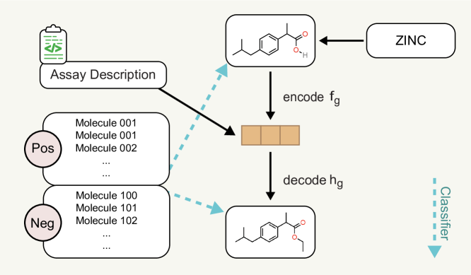
Figure 8: Pipeline for binding-affinity-based molecule editing. The input molecules are randomly sampled from ZINC, and the text prompt is the assay description. For evaluation, the small molecules for each assay are used to train a binary classifier, and two types of models (random forest and logistic regression) are considered.

The hit ratio results are shown in Table 17. Notice that to better prove the validity of our results, we train two classifiers for each assay: random forest (RF) and logistic regression (LR), with the fingerprint as featurization. the $\Delta$ is 0.

Table 17: Results on six ChEMBL assay editing. Each ChEMBL assay is a binary task and we train a classifier to obtain the confidence score of each molecule (input and output molecules). The inputs are 200 molecules randomly sampled from ZINC, and the evaluation is the hit ratio of the confidence change. The latent optimization is the text-based molecule editing with MoleculeSTM, with the SMILES string and the molecular graph, respectively.

baseline latent optimization ChEMBL ID Random PCA High Variance GS-Mutate SMILES Graph 1613777 RF 44.99 $\pm$ 2.08 44.49 $\pm$ 1.22 44.45 $\pm$ 1.01 39.17 $\pm$ 3.66 48.70 $\pm$ 2.06 44.53 $\pm$ 1.60 LR 47.34 $\pm$ 5.53 49.13 $\pm$ 0.86 49.69 $\pm$ 6.75 51.50 $\pm$ 2.86 54.09 $\pm$ 1.94 50.55 $\pm$ 3.14 1613797 RF 44.76 $\pm$ 2.18 46.25 $\pm$ 0.97 46.92 $\pm$ 3.34 46.67 $\pm$ 1.55 55.03 $\pm$ 2.23 49.03 $\pm$ 0.03 LR 48.40 $\pm$ 3.71 49.92 $\pm$ 4.31 48.67 $\pm$ 1.64 49.17 $\pm$ 3.01 57.98 $\pm$ 3.34 54.95 $\pm$ 3.74 2114713 RF 39.87 $\pm$ 2.32 42.91 $\pm$ 2.64 42.19 $\pm$ 3.68 41.33 $\pm$ 1.25 49.20 $\pm$ 2.11 60.93 $\pm$ 2.53 LR 51.39 $\pm$ 1.15 52.62 $\pm$ 1.64 52.24 $\pm$ 1.07 50.50 $\pm$ 1.47 56.93 $\pm$ 3.67 58.77 $\pm$ 2.41 1613838 RF 44.49 $\pm$ 1.48 44.71 $\pm$ 1.80 45.30 $\pm$ 2.47 36.00 $\pm$ 2.68 43.94 $\pm$ 3.75 49.13 $\pm$ 2.52 LR 50.22 $\pm$ 4.23 49.73 $\pm$ 2.33 44.69 $\pm$ 2.41 41.33 $\pm$ 3.17 47.50 $\pm$ 2.28 56.13 $\pm$ 1.50 1614236 RF 41.33 $\pm$ 3.59 42.28 $\pm$ 1.91 42.85 $\pm$ 2.88 45.33 $\pm$ 1.65 57.90 $\pm$ 2.39 35.71 $\pm$ 4.19 LR 46.57 $\pm$ 0.51 49.34 $\pm$ 1.80 50.62 $\pm$ 3.86 56.00 $\pm$ 1.08 65.78 $\pm$ 5.67 46.36 $\pm$ 2.53 1613903 RF 44.28 $\pm$ 0.77 43.83 $\pm$ 2.65 42.00 $\pm$ 3.19 46.17 $\pm$ 0.85 56.82 $\pm$ 3.96 58.70 $\pm$ 1.43 LR 53.94 $\pm$ 3.30 48.63 $\pm$ 4.49 56.19 $\pm$ 2.51 56.33 $\pm$ 0.94 58.31 $\pm$ 2.98 64.64 $\pm$ 5.23

Then we add docking for visualization in Figure 9. We choose the ChEMBL 1613777 with the available PDB structure. In specific, we first extract the output molecules using MoleculeSTM with confidence (RF and LR) higher than the ones generated with baselines. Then we run the molecular docking software for the results. The details of docking settings are listed below.

• We use Merck molecular force field (MMFF) [80] provided in RDKit [81] to embed (generate) 3D conformers for each molecule. The dielectric constant is set to be 80 and the maximum iteration of optimization is 1000 for MMFF, and the up-to-5 conformers from each molecule are used for further analysis.

• For the binding target, we consider assay P450 (CYP) 2C19 [82] (CHEMBL id: 1613777) and select the corresponding crystal structure available in the Protein Data Bank (PDB) (PDB id: 4GQS). Further, we take chain A for docking running. Later for the binding, the binding pockets are aligned with the original ligand in the crystal structure of PDB complexes: the center is set to (-81.48, 16.55, -41.6), and the box is (20.0, 23.0, 25.0).

• Then we take a preprocessing step to complement the hydrogen atoms and add partial charges. We utilize meeko v0.3.3 for small molecules and AutoDock Flexible Receptor (ADFR) suite v1.2 for proteins.

• For docking, we use AutoDock Vina v1.2.3 [83]. Each molecule conformer is docked with exhausitiveness being 32, and the pose with the best (lowest) docking score is picked and used for visualization. For visualization, we use UCSF Chimera.

Figure 9: Two sets of docking visualization for binding-affinity-based molecule editing. The text prompt is from ChEMBL 1613777 (“This molecule is tested positive in an assay that are inhibitors and substrates of an enzyme protein. It uses molecular oxygen inserting one oxygen atom into a substrate, and reducing the second into a water molecule.”). For visualization, the input molecule and output molecules with GS and MoleculeSTM are displayed. It is observed that MoleculeSTM can generate molecules with the lowest docking scores (with the most Hydrogen bonds, and marked in red dashed lines). In set 1 (a), the output molecules are sharing the same molecule scaffold. In set 2 (b), the motif of the output molecule using MoleculeSTM also changes.

C.5 Drug Relevance Editing

As a proof-of-concept, we further take four editing tasks on common drug editing. The text prompts used here are to make the input molecules look like an existing drug, e.g., “This molecule looks like Penicillin.” Following the Methods section, the satisfy function used is the Tanimoto similarity, and the threshold $\Delta$ takes the value of 0 and 0.05.

Table 18: Results on four common drug molecule editing. The inputs are 200 molecules randomly sampled from ZINC, and the evaluation is the hit ratio on the increase of the Tanimoto similarity with the common drug. The latent optimization is text-based molecule editing with MoleculeSTM, with the SMILES string and the molecular graph, respectively.

baseline latent optimization $\Delta$ Random PCA High Variance GS-Mutate SMILES Graph This molecule looks like Penicillin. 0 43.61 $\pm$ 2.23 46.51 $\pm$ 3.02 44.42 $\pm$ 3.56 28.67 $\pm$ 0.94 58.13 $\pm$ 0.97 50.91 $\pm$ 2.80 0.05 0.69 $\pm$ 0.55 0.23 $\pm$ 0.32 0.89 $\pm$ 0.30 0.67 $\pm$ 0.62 11.01 $\pm$ 0.58 3.64 $\pm$ 0.57 This molecule looks like Aspirin. 0 43.82 $\pm$ 1.41 43.12 $\pm$ 5.35 44.63 $\pm$ 3.33 25.00 $\pm$ 2.16 40.13 $\pm$ 1.33 54.05 $\pm$ 3.58 0.05 2.99 $\pm$ 0.38 3.08 $\pm$ 0.82 2.45 $\pm$ 0.33 0.33 $\pm$ 0.47 4.28 $\pm$ 1.22 10.84 $\pm$ 1.26 This molecule looks like Caffeine. 0 42.71 $\pm$ 3.16 40.33 $\pm$ 0.71 40.64 $\pm$ 3.89 26.17 $\pm$ 1.31 46.08 $\pm$ 3.81 51.01 $\pm$ 1.22 0.05 0.69 $\pm$ 0.01 0.23 $\pm$ 0.32 0.44 $\pm$ 0.31 0.33 $\pm$ 0.24 1.61 $\pm$ 0.67 0.61 $\pm$ 0.01 This molecule looks like Dopamine. 0 42.00 $\pm$ 3.08 42.50 $\pm$ 2.12 41.33 $\pm$ 2.86 30.50 $\pm$ 1.63 47.00 $\pm$ 4.11 55.50 $\pm$ 2.73 0.05 0.00 $\pm$ 0.00 0.44 $\pm$ 0.31 0.22 $\pm$ 0.31 0.83 $\pm$ 0.24 2.30 $\pm$ 0.44 6.24 $\pm$ 0.56

C.6 Case Studies on Neighborhood Searching for Patent Drug Molecules

To demonstrate the utility of text-based molecule editing, we show three case studies of generating approved drugs from their analogs. Lead optimization is a critical phase of drug discovery in which closely related compounds are made based on the lead molecule, aiming to improve its efficacy and DMPK (drug metabolism and pharmacokinetics) properties and ultimately identifying a drug candidate [84]. A text prompt calling for greater drug-like properties will thus be informative towards improving on deficiencies in the lead molecule and accelerating drug discovery research.

In specific here, the input molecules are the patented analogs of each approved drug molecule, and the input text prompt is single-objective, like the ones in Section C.2. The goal here is to check if the approved drugs can be successfully generated as the output molecules, with the structural changes consistent with the property improvement reflected in the text prompt. For example, in Table 19 (a), Erlotinib is successfully generated from an analog by replacing an imidazole substituent to a methoxy group [85]. This change reflects a tPSA drop from 83 to 75, consistent with the text prompt indicating a higher permeability. Table 19 (b) generates Celecoxib from its amino-substituted derivative [86], where the removal of the amino group yields a greater intestinal permeability of the molecule leading to higher bioavailability. Bioavailability is the fraction of a drug molecule that reaches the systemic circulation, a key factor for oral drug absorption [87]. Finally, Table 19 (c) illustrates how potential metabolic liabilities in a molecule can be addressed via text-based editing. A text calling for a metabolically stable molecule successfully turns a trimethoxy arene to a dimethoxy arene in Donepezil [88], where the former represents an electron-rich aromatic compound known to undergo oxidative phase I metabolisms [89].

Table 19: Visualization on three single-objective molecule editing on drug analogs that generates approved drugs based on the text prompt. The pink and blue regions highlight the modified structure in the input and output molecules, respectively.

(a) Prompt: This molecule has high permeability. (b) Prompt: This molecule has high bioavailability. (c) Prompt: This molecule is metabolically stable. Input Molecule Output Molecule Input Molecule Output Molecule Input Molecule Output Molecule CAS: 183320-43-6 Tarceva (Erlotinib) CAS: 170570-28-2 Celebrex (Celecoxib) CAS: 120013-52-7 Aricept (Donepezil)

Appendix D Downstream: Molecular Property Prediction

In this section, we review two main categories of datasets used for molecular property prediction downstream tasks from MoleculeNet and molecule benchmarking works [90, 91].

Molecular Property: Pharmacology

The Blood-Brain Barrier Penetration (BBBP) [92] dataset measures whether a molecule will penetrate the central nervous system. All three toxicity-related datasets, Tox21 [93], ToxCast [90], and ClinTox [94] are related to the toxicity of molecular compounds. The Side Effect Resource (SIDER) [95] dataset stores the adverse drug reactions on a marketed drug database.

Molecular Property: Biophysics

Maximum Unbiased Validation (MUV) [96] is another sub-database from PCBA, and is obtained by applying a refined nearest neighbor analysis. HIV is from the Drug Therapeutics Program (DTP) AIDS Antiviral Screen [97], and it aims at predicting the inhibition of HIV replication. BACE measures the binding results for a set of inhibitors of $\beta$-secretase 1 (BACE-1) and is gathered in MoleculeNet [90].

Table 20: Summary for the molecule chemical datasets.

Dataset	Task	# Tasks	# Molecules
BBBP	Classification	1	2,039
Tox21	Classification	12	7,831
ToxCast	Classification	617	8,576
Sider	Classification	27	1,427
ClinTox	Classification	2	1,478
MUV	Classification	17	93,087
HIV	Classification	1	41,127
Bace	Classification	1	1,513

For data splitting, we adopt the scaffold splitting [90]. Scaffold measures the skeleton structure of molecules, and scaffold splitting means we will put the molecules with more common scaffolds into training, and the rest into validation and test, so as to mimic the out-of-distribution (OOD) setting. The OOD setting is more common in real scenarios and thus is preferred to test the pretrained molecule representation power.

Implementation Details

For the SMILES string, we use MegaMolBART [67] as the backbone Transformer model. For the molecular graph, we use the same backbone GIN model, and we use rich features (as used for the regression tasks in GraphMVP [70]). We list the main hyperparameters below.

Table 21: Hyperparameter specifications for molecular property prediction.

Hyperparameter Value Pretraining Baseline epochs {100} learning rate {1e-3} weight decay {0} Downstream epochs {100} learning rate {1e-3, 5e-4} weight decay {0}

Choice of backbone models. We want to clarify that the MoleculeSTM is agnostic to the backbone encoders for each modality, e.g., the molecule representation model.

• For the backbone model, we use the GIN model as the fixed 2D GNN backbone encoder. In other words, the performance of MoleculeSTM is limited by the 2D backbone model.

• In the molecule pretraining research line, (e.g., AttrMask [98], MolCLR [99], GraphMVP [70], MoleculeSDE [100]), all of these works adopt GIN as the 2D backbone model, serving as a control to test the effectiveness of various pretraining algorithms. This is a similar case for our proposed MoleculeSTM.

• In the future, we would like to explore more advanced GNN models on molecules.

References

- [1] Thomas Sullivan “A tough road: cost to develop one new drug is $2.6 billion; approval rate for drugs entering clinical development is less than 12%” In Policy & Medicine, 2019
- [2] Atanas Patronov, Kostas Papadopoulos and Ola Engkvist “Has artificial intelligence impacted drug discovery?” In Artificial Intelligence in Drug Design Springer, 2022, pp. 153–176
- [3] Madura KP Jayatunga, Wen Xie, Ludwig Ruder, Ulrik Schulze and Christoph Meier “AI in small-molecule drug discovery: A coming wave” In Nat. Rev. Drug Discov 21, 2022, pp. 175–176
- [4] John Jumper, Richard Evans, Alexander Pritzel, Tim Green, Michael Figurnov, Olaf Ronneberger, Kathryn Tunyasuvunakool, Russ Bates, Augustin Žídek, Anna Potapenko, Alex Bridgland, Clemens Meyer, Simon A.. Kohl, Andrew J. Ballard, Andrew Cowie, Bernardino Romera-Paredes, Stanislav Nikolov, Rishub Jain, Jonas Adler, Trevor Back, Stig Petersen, David Reiman, Ellen Clancy, Michal Zielinski, Martin Steinegger, Michalina Pacholska, Tamas Berghammer, Sebastian Bodenstein, David Silver, Oriol Vinyals, Andrew W. Senior, Koray Kavukcuoglu, Pushmeet Kohli and Demis Hassabis “Highly accurate protein structure prediction with AlphaFold” In Nature 596.7873 Nature Publishing Group, 2021, pp. 583–589
- [5] Sebastian G. Rohrer and Knut Baumann “Maximum Unbiased Validation (MUV) Data Sets for Virtual Screening Based on PubChem Bioactivity Data” PMID: 19161251 In Journal of Chemical Information and Modeling 49.2, 2009, pp. 169–184 DOI: 10.1021/ci8002649
- [6] Shengchao Liu, Moayad Alnammi, Spencer S Ericksen, Andrew F Voter, Gene E Ananiev, James L Keck, F Michael Hoffmann, Scott A Wildman and Anthony Gitter “Practical model selection for prospective virtual screening” In Journal of chemical information and modeling 59.1 ACS Publications, 2018, pp. 282–293
- [7] David K Duvenaud, Dougal Maclaurin, Jorge Iparraguirre, Rafael Bombarell, Timothy Hirzel, Alán Aspuru-Guzik and Ryan P Adams “Convolutional networks on graphs for learning molecular fingerprints” In Advances in neural information processing systems 28, 2015
- [8] Shengchao Liu, Mehmet F Demirel and Yingyu Liang “N-Gram Graph: Simple Unsupervised Representation for Graphs, with Applications to Molecules” In Advances in neural information processing systems 32, 2019
- [9] Zhenqin Wu, Bharath Ramsundar, Evan N Feinberg, Joseph Gomes, Caleb Geniesse, Aneesh S Pappu, Karl Leswing and Vijay Pande “MoleculeNet: a benchmark for molecular machine learning” In Chemical science 9.2 Royal Society of Chemistry, 2018, pp. 513–530
- [10] Wengong Jin, Regina Barzilay and Tommi Jaakkola “Hierarchical generation of molecular graphs using structural motifs” In International conference on machine learning, 2020, pp. 4839–4848 PMLR
- [11] Ross Irwin, Spyridon Dimitriadis, Jiazhen He and Esben Jannik Bjerrum “Chemformer: a pre-trained transformer for computational chemistry” In Machine Learning: Science and Technology 3.1 IOP Publishing, 2022, pp. 015022
- [12] Zichao Wang, Weili Nie, Zhuoran Qiao, Chaowei Xiao, Richard Baraniuk and Anima Anandkumar “Retrieval-based Controllable Molecule Generation” In arXiv preprint arXiv:2208.11126, 2022
- [13] Shengchao Liu, Chengpeng Wang, Weili Nie, Hanchen Wang, Jiarui Lu, Bolei Zhou and Jian Tang “GraphCG: Unsupervised Discovery of Steerable Factors in Graphs” In NeurIPS 2022 Workshop: New Frontiers in Graph Learning, 2022 URL: https://openreview.net/forum?id=BhR44NzeK_1
- [14] Mario Krenn, Florian Häse, AkshatKumar Nigam, Pascal Friederich and Alan Aspuru-Guzik “Self-referencing embedded strings (SELFIES): A 100% robust molecular string representation” In Machine Learning: Science and Technology 1.4 IOP Publishing, 2020, pp. 045024
- [15] Keyulu Xu, Weihua Hu, Jure Leskovec and Stefanie Jegelka “How powerful are graph neural networks?” In arXiv preprint arXiv:1810.00826, 2018
- [16] Kristof T Schütt, Huziel E Sauceda, P-J Kindermans, Alexandre Tkatchenko and K-R Müller “Schnet–a deep learning architecture for molecules and materials” In The Journal of Chemical Physics 148.24 AIP Publishing LLC, 2018, pp. 241722
- [17] Victor Garcia Satorras, Emiel Hoogeboom and Max Welling “E (n) equivariant graph neural networks” In arXiv preprint arXiv:2102.09844, 2021
- [18] Kenneth Atz, Francesca Grisoni and Gisbert Schneider “Geometric deep learning on molecular representations” In Nature Machine Intelligence 3.12 Nature Publishing Group, 2021, pp. 1023–1032
- [19] Yuanfeng Ji, Lu Zhang, Jiaxiang Wu, Bingzhe Wu, Long-Kai Huang, Tingyang Xu, Yu Rong, Lanqing Li, Jie Ren and Ding Xue “DrugOOD: Out-of-Distribution (OOD) Dataset Curator and Benchmark for AI-aided Drug Discovery–A Focus on Affinity Prediction Problems with Noise Annotations” In arXiv preprint arXiv:2201.09637, 2022
- [20] John J Irwin, Teague Sterling, Michael M Mysinger, Erin S Bolstad and Ryan G Coleman “ZINC: a free tool to discover chemistry for biology” In Journal of chemical information and modeling 52.7 ACS Publications, 2012, pp. 1757–1768
- [21] Weihua Hu, Bowen Liu, Joseph Gomes, Marinka Zitnik, Percy Liang, Vijay Pande and Jure Leskovec “Strategies for pre-training graph neural networks” In International Conference on Learning Representations, ICLR, 2020
- [22] Shengchao Liu, Hongyu Guo and Jian Tang “Molecular geometry pretraining with se (3)-invariant denoising distance matching” In arXiv preprint arXiv:2206.13602, 2022
- [23] Hugo Larochelle, Dumitru Erhan and Yoshua Bengio “Zero-data learning of new tasks.” In AAAI 1.2, 2008, pp. 3
- [24] Alec Radford, Jong Wook Kim, Chris Hallacy, Aditya Ramesh, Gabriel Goh, Sandhini Agarwal, Girish Sastry, Amanda Askell, Pamela Mishkin and Jack Clark “Learning transferable visual models from natural language supervision” In International Conference on Machine Learning, 2021, pp. 8748–8763 PMLR
- [25] Alex Nichol, Prafulla Dhariwal, Aditya Ramesh, Pranav Shyam, Pamela Mishkin, Bob McGrew, Ilya Sutskever and Mark Chen “Glide: Towards photorealistic image generation and editing with text-guided diffusion models” In arXiv preprint arXiv:2112.10741, 2021
- [26] Aditya Ramesh, Prafulla Dhariwal, Alex Nichol, Casey Chu and Mark Chen “Hierarchical text-conditional image generation with clip latents” In arXiv preprint arXiv:2204.06125, 2022
- [27] Or Patashnik, Zongze Wu, Eli Shechtman, Daniel Cohen-Or and Dani Lischinski “Styleclip: Text-driven manipulation of stylegan imagery” In Proceedings of the IEEE/CVF International Conference on Computer Vision, 2021, pp. 2085–2094
- [28] Shuang Li, Xavier Puig, Yilun Du, Clinton Wang, Ekin Akyurek, Antonio Torralba, Jacob Andreas and Igor Mordatch “Pre-trained language models for interactive decision-making” In arXiv preprint arXiv:2202.01771, 2022
- [29] Linxi Fan, Guanzhi Wang, Yunfan Jiang, Ajay Mandlekar, Yuncong Yang, Haoyi Zhu, Andrew Tang, De-An Huang, Yuke Zhu and Anima Anandkumar “Minedojo: Building open-ended embodied agents with internet-scale knowledge” In arXiv preprint arXiv:2206.08853, 2022
- [30] Zheni Zeng, Yuan Yao, Zhiyuan Liu and Maosong Sun “A deep-learning system bridging molecule structure and biomedical text with comprehension comparable to human professionals” In Nature communications 13.1 Nature Publishing Group, 2022, pp. 1–11
- [31] Shengchao Liu, Hanchen Wang, Weiyang Liu, Joan Lasenby, Hongyu Guo and Jian Tang “Pre-training Molecular Graph Representation with 3D Geometry” In International Conference on Learning Representations, 2022 URL: https://openreview.net/forum?id=xQUe1pOKPam
- [32] Iz Beltagy, Kyle Lo and Arman Cohan “SciBERT: Pretrained Language Model for Scientific Text” In EMNLP, 2019 eprint: arXiv:1903.10676
- [33] Aaron van den Oord, Yazhe Li and Oriol Vinyals “Representation learning with contrastive predictive coding” In arXiv preprint arXiv:1807.03748, 2018
- [34] Sunghwan Kim, Jie Chen, Tiejun Cheng, Asta Gindulyte, Jia He, Siqian He, Qingliang Li, Benjamin A Shoemaker, Paul A Thiessen and Bo Yu “PubChem in 2021: new data content and improved web interfaces” In Nucleic acids research 49.D1 Oxford University Press, 2021, pp. D1388–D1395
- [35] James P Hughes, Stephen Rees, S Barrett Kalindjian and Karen L Philpott “Principles of early drug discovery” In British journal of pharmacology 162.6 Wiley Online Library, 2011, pp. 1239–1249
- [36] Ashish Vaswani, Noam Shazeer, Niki Parmar, Jakob Uszkoreit, Llion Jones, Aidan N Gomez, Łukasz Kaiser and Illia Polosukhin “Attention is all you need” In Advances in neural information processing systems 30, 2017
- [37] Jacob Devlin, Ming-Wei Chang, Kenton Lee and Kristina Toutanova “Bert: Pre-training of deep bidirectional transformers for language understanding” In arXiv preprint arXiv:1810.04805, 2018
- [38] Xiuye Gu, Tsung-Yi Lin, Weicheng Kuo and Yin Cui “Open-vocabulary object detection via vision and language knowledge distillation” In arXiv preprint arXiv:2104.13921, 2021
- [39] David S Wishart, Yannick D Feunang, An C Guo, Elvis J Lo, Ana Marcu, Jason R Grant, Tanvir Sajed, Daniel Johnson, Carin Li and Zinat Sayeeda “DrugBank 5.0: a major update to the DrugBank database for 2018” In Nucleic acids research 46.D1 Oxford University Press, 2018, pp. D1074–D1082
- [40] David Mendez, Anna Gaulton, A Patrícia Bento, Jon Chambers, Marleen De Veij, Eloy Félix, María Paula Magariños, Juan F Mosquera, Prudence Mutowo, Michał Nowotka, María Gordillo-Marañón, Fiona Hunter, Laura Junco, Grace Mugumbate, Milagros Rodriguez-Lopez, Francis Atkinson, Nicolas Bosc, Chris J Radoux, Aldo Segura-Cabrera, Anne Hersey and Andrew R Leach “ChEMBL: towards direct deposition of bioassay data” In Nucleic Acids Research 47.D1, 2018, pp. D930–D940 DOI: 10.1093/nar/gky1075
- [41] Jan H Jensen “A graph-based genetic algorithm and generative model/Monte Carlo tree search for the exploration of chemical space” In Chemical science 10.12 Royal Society of Chemistry, 2019, pp. 3567–3572
- [42] John J Talley, Thomas D Penning, Paul W Collins, Donald J Rogier Jr, James W Malecha, Julie M Miyashiro, Stephen R Bertenshaw, Ish K Khanna, Matthew J Graneto and Roland S Rogers “Substituted pyrazolyl benzenesulfonamides for the treatment of inflammation” US Patent 5,760,068 Google Patents, 1998
- [43] David Dahlgren and Hans Lennernäs “Intestinal Permeability and Drug Absorption: Predictive Experimental, Computational and In Vivo Approaches” In Pharmaceutics 11.8, 2019 DOI: 10.3390/pharmaceutics11080411
- [44] Gordon Guroff, Jean Renson, Sidney Udenfriend, John W Daly, Donald M Jerina and Bernhard Witkop “Hydroxylation-Induced Migration: The NIH Shift: Recent experiments reveal an unexpected and general result of enzymatic hydroxylation of aromatic compounds.” In Science 157.3796 American Association for the Advancement of Science, 1967, pp. 1524–1530
- [45] Andrew P Bradley “The use of the area under the ROC curve in the evaluation of machine learning algorithms” In Pattern recognition 30.7 Elsevier, 1997, pp. 1145–1159
- [46] Fan-Yun Sun, Jordan Hoffmann, Vikas Verma and Jian Tang “Infograph: Unsupervised and semi-supervised graph-level representation learning via mutual information maximization” In International Conference on Learning Representations, ICLR, 2020
- [47] Yuyang Wang, Jianren Wang, Zhonglin Cao and Amir Barati Farimani “Molclr: Molecular contrastive learning of representations via graph neural networks” In arXiv preprint arXiv:2102.10056, 2021
- [48] Kyle Lo, Lucy Lu Wang, Mark Neumann, Rodney Kinney and Dan S Weld “S2ORC: The semantic scholar open research corpus” In arXiv preprint arXiv:1911.02782, 2019
- [49] Teague Sterling and John J Irwin “ZINC 15–ligand discovery for everyone” In Journal of chemical information and modeling 55.11 ACS Publications, 2015, pp. 2324–2337
- [50] Simon Axelrod and Rafael Gomez-Bombarelli “GEOM, energy-annotated molecular conformations for property prediction and molecular generation” In Scientific Data 9.1 Nature Publishing Group, 2022, pp. 1–14
- [51] Saurabh Aggarwal “Targeted cancer therapies” In Nature reviews. Drug discovery 9.6 Nature Publishing Group, 2010, pp. 427
- [52] Emre Guney “Reproducible drug repurposing: When similarity does not suffice” In Pacific Symposium on Biocomputing 2017, 2017, pp. 132–143 World Scientific
- [53] Peter Ertl, Eva Altmann and Jeffrey M McKenna “The most common functional groups in bioactive molecules and how their popularity has evolved over time” In Journal of medicinal chemistry 63.15, 2020, pp. 8408–8418
- [54] Hans-Joachim Böhm, Alexander Flohr and Martin Stahl “Scaffold hopping” In Drug discovery today: Technologies 1.3, 2004, pp. 217–224
- [55] Ye Hu, Dagmar Stumpfe and Jurgen Bajorath “Recent advances in scaffold hopping: miniperspective” In Journal of medicinal chemistry 60.4, 2017, pp. 1238–1246
- [56] Jürgen Drews “Drug discovery: a historical perspective” In Science 287.5460, 2000, pp. 1960–1964
- [57] Laurent Gomez “Decision making in medicinal chemistry: The power of our intuition” In ACS Medicinal Chemistry Letters 9.10, 2018, pp. 956–958
- [58] Albert Leo, Corwin Hansch and David Elkins “Partition coefficients and their uses” In Chemical Reviews 71.6, 1971, pp. 525–616 DOI: 10.1021/cr60274a001
- [59] G Richard Bickerton, Gaia V Paolini, Jérémy Besnard, Sorel Muresan and Andrew L Hopkins “Quantifying the chemical beauty of drugs” In Nature chemistry 4.2 Nature Publishing Group, 2012, pp. 90–98
- [60] Peter Ertl, Bernhard Rohde and Paul Selzer “Fast Calculation of Molecular Polar Surface Area as a Sum of Fragment-Based Contributions and Its Application to the Prediction of Drug Transport Properties” PMID: 11020286 In Journal of Medicinal Chemistry 43.20, 2000, pp. 3714–3717 DOI: 10.1021/jm000942e
- [61] Darko Butina “Unsupervised Data Base Clustering Based on Daylight’s Fingerprint and Tanimoto Similarity: A Fast and Automated Way To Cluster Small and Large Data Sets” In Journal of Chemical Information and Computer Sciences 39.4, 1999, pp. 747–750 DOI: 10.1021/ci9803381
- [62] Shengchao Liu, Weili Nie, Chengpeng Wang, Jiarui Lu, Zhuoran Qiao, Ling Liu, Jian Tang, Chaowei Xiao and Anima Anandkumar “Multi-modal Molecule Structure-text Model for Text-based Editing and Retrieval” Zenodo, 2023 DOI: 10.5281/zenodo.8303265
- [63] Sunghwan Kim, Jie Chen, Tiejun Cheng, Asta Gindulyte, Jia He, Siqian He, Qingliang Li, Benjamin A Shoemaker, Paul A Thiessen and Bo Yu “PubChem in 2021: new data content and improved web interfaces” In Nucleic acids research 49.D1 Oxford University Press, 2021, pp. D1388–D1395
- [64] Iz Beltagy, Kyle Lo and Arman Cohan “SciBERT: Pretrained Language Model for Scientific Text” In EMNLP, 2019 eprint: arXiv:1903.10676
- [65] Waleed Ammar, Dirk Groeneveld, Chandra Bhagavatula, Iz Beltagy, Miles Crawford, Doug Downey, Jason Dunkelberger, Ahmed Elgohary, Sergey Feldman and Vu Ha “Construction of the literature graph in semantic scholar” In arXiv preprint arXiv:1805.02262, 2018
- [66] M Honnibal, I Montani and S Van Landeghem “Boyd” In A. spaCy: industrial-strength natural language processing in Python, 2020
- [67] Ross Irwin, Spyridon Dimitriadis, Jiazhen He and Esben Jannik Bjerrum “Chemformer: a pre-trained transformer for computational chemistry” In Machine Learning: Science and Technology 3.1 IOP Publishing, 2022, pp. 015022
- [68] Teague Sterling and John J Irwin “ZINC 15–ligand discovery for everyone” In Journal of chemical information and modeling 55.11 ACS Publications, 2015, pp. 2324–2337
- [69] Keyulu Xu, Weihua Hu, Jure Leskovec and Stefanie Jegelka “How powerful are graph neural networks?” In arXiv preprint arXiv:1810.00826, 2018
- [70] Shengchao Liu, Hanchen Wang, Weiyang Liu, Joan Lasenby, Hongyu Guo and Jian Tang “Pre-training Molecular Graph Representation with 3D Geometry” In International Conference on Learning Representations, 2022 URL: https://openreview.net/forum?id=xQUe1pOKPam
- [71] Simon Axelrod and Rafael Gomez-Bombarelli “GEOM, energy-annotated molecular conformations for property prediction and molecular generation” In Scientific Data 9.1 Nature Publishing Group, 2022, pp. 1–14
- [72] Jacob Devlin, Ming-Wei Chang, Kenton Lee and Kristina Toutanova “Bert: Pre-training of deep bidirectional transformers for language understanding” In arXiv preprint arXiv:1810.04805, 2018
- [73] Aaron van den Oord, Yazhe Li and Oriol Vinyals “Representation learning with contrastive predictive coding” In arXiv preprint arXiv:1807.03748, 2018
- [74] Kaveh Hassani and Amir Hosein Khasahmadi “Contrastive multi-view representation learning on graphs” In International Conference on Machine Learning, 2020, pp. 4116–4126 PMLR
- [75] Chitwan Saharia, William Chan, Saurabh Saxena, Lala Li, Jay Whang, Emily Denton, Seyed Kamyar Seyed Ghasemipour, Burcu Karagol Ayan, S Sara Mahdavi and Rapha Gontijo Lopes “Photorealistic Text-to-Image Diffusion Models with Deep Language Understanding” In arXiv preprint arXiv:2205.11487, 2022
- [76] David S Wishart, Yannick D Feunang, An C Guo, Elvis J Lo, Ana Marcu, Jason R Grant, Tanvir Sajed, Daniel Johnson, Carin Li and Zinat Sayeeda “DrugBank 5.0: a major update to the DrugBank database for 2018” In Nucleic acids research 46.D1 Oxford University Press, 2018, pp. D1074–D1082
- [77] Tero Karras, Samuli Laine and Timo Aila “A style-based generator architecture for generative adversarial networks” In Proceedings of the IEEE/CVF conference on computer vision and pattern recognition, 2019, pp. 4401–4410
- [78] Shengchao Liu, Chengpeng Wang, Weili Nie, Hanchen Wang, Jiarui Lu, Bolei Zhou and Jian Tang “GraphCG: Unsupervised Discovery of Steerable Factors in Graphs” In NeurIPS 2022 Workshop: New Frontiers in Graph Learning, 2022 URL: https://openreview.net/forum?id=BhR44NzeK_1
- [79] David Mendez, Anna Gaulton, A Patrícia Bento, Jon Chambers, Marleen De Veij, Eloy Félix, María Paula Magariños, Juan F Mosquera, Prudence Mutowo, Michał Nowotka, María Gordillo-Marañón, Fiona Hunter, Laura Junco, Grace Mugumbate, Milagros Rodriguez-Lopez, Francis Atkinson, Nicolas Bosc, Chris J Radoux, Aldo Segura-Cabrera, Anne Hersey and Andrew R Leach “ChEMBL: towards direct deposition of bioassay data” In Nucleic Acids Research 47.D1, 2018, pp. D930–D940 DOI: 10.1093/nar/gky1075
- [80] Thomas A Halgren “Merck molecular force field. I. Basis, form, scope, parameterization, and performance of MMFF94” In Journal of computational chemistry 17.5-6 Wiley Online Library, 1996, pp. 490–519
- [81] Greg Landrum “RDKit: A software suite for cheminformatics, computational chemistry, and predictive modeling” Academic Press Cambridge, 2013
- [82] R Leila Reynald, Stefaan Sansen, C David Stout and Eric F Johnson “Structural Characterization of Human Cytochrome P450 2C19: ACTIVE SITE DIFFERENCES BETWEEN P450s 2C8, 2C9, AND 2C19” In Journal of Biological Chemistry 287.53 ASBMB, 2012, pp. 44581–44591
- [83] Oleg Trott and Arthur J Olson “AutoDock Vina: improving the speed and accuracy of docking with a new scoring function, efficient optimization, and multithreading” In Journal of computational chemistry 31.2 Wiley Online Library, 2010, pp. 455–461
- [84] James P Hughes, Stephen Rees, S Barrett Kalindjian and Karen L Philpott “Principles of early drug discovery” In British journal of pharmacology 162.6 Wiley Online Library, 2011, pp. 1239–1249
- [85] Rodney Caughren Schnur and Lee Daniel Arnold “Alkynyl and azido-substituted 4-anilinoquinazolines” US Patent 5,747,498 Google Patents, 1998
- [86] John J Talley, Thomas D Penning, Paul W Collins, Donald J Rogier Jr, James W Malecha, Julie M Miyashiro, Stephen R Bertenshaw, Ish K Khanna, Matthew J Graneto and Roland S Rogers “Substituted pyrazolyl benzenesulfonamides for the treatment of inflammation” US Patent 5,760,068 Google Patents, 1998
- [87] David Dahlgren and Hans Lennernäs “Intestinal Permeability and Drug Absorption: Predictive Experimental, Computational and In Vivo Approaches” In Pharmaceutics 11.8, 2019 DOI: 10.3390/pharmaceutics11080411
- [88] Hachiro Sugimoto, Youichi Iimura, Yoshiharu Yamanishi and Kiyomi Yamatsu “Synthesis and Structure-Activity Relationships of Acetylcholinesterase Inhibitors: 1-Benzyl-4-[(5,6-dimethoxy-1-oxoindan-2-yl)methyl]piperidine Hydrochloride and Related Compounds” PMID: 7490731 In Journal of Medicinal Chemistry 38.24, 1995, pp. 4821–4829 DOI: 10.1021/jm00024a009
- [89] Gordon Guroff, Jean Renson, Sidney Udenfriend, John W Daly, Donald M Jerina and Bernhard Witkop “Hydroxylation-Induced Migration: The NIH Shift: Recent experiments reveal an unexpected and general result of enzymatic hydroxylation of aromatic compounds.” In Science 157.3796 American Association for the Advancement of Science, 1967, pp. 1524–1530
- [90] Zhenqin Wu, Bharath Ramsundar, Evan N Feinberg, Joseph Gomes, Caleb Geniesse, Aneesh S Pappu, Karl Leswing and Vijay Pande “MoleculeNet: a benchmark for molecular machine learning” In Chemical science 9.2 Royal Society of Chemistry, 2018, pp. 513–530
- [91] Hanchen Wang, Jean Kaddour, Shengchao Liu, Jian Tang, Matt Kusner, Joan Lasenby and Qi Liu “Evaluating Self-Supervised Learning for Molecular Graph Embeddings”, 2022 URL: https://openreview.net/forum?id=ctX2eXYIW3
- [92] Ines Filipa Martins, Ana L Teixeira, Luis Pinheiro and Andre O Falcao “A Bayesian approach to in silico blood-brain barrier penetration modeling” In Journal of chemical information and modeling 52.6 ACS Publications, 2012, pp. 1686–1697
- [93] Tox21 Data Challenge “Tox21 Data Challenge 2014” In https://tripod.nih.gov/tox21/challenge/, 2014
- [94] Kaitlyn M Gayvert, Neel S Madhukar and Olivier Elemento “A data-driven approach to predicting successes and failures of clinical trials” In Cell chemical biology 23.10 Elsevier, 2016, pp. 1294–1301
- [95] Michael Kuhn, Ivica Letunic, Lars Juhl Jensen and Peer Bork “The SIDER database of drugs and side effects” In Nucleic acids research 44.D1 Oxford University Press, 2015, pp. D1075–D1079
- [96] Sebastian G. Rohrer and Knut Baumann “Maximum Unbiased Validation (MUV) Data Sets for Virtual Screening Based on PubChem Bioactivity Data” PMID: 19161251 In Journal of Chemical Information and Modeling 49.2, 2009, pp. 169–184 DOI: 10.1021/ci8002649
- [97] Daniel Zaharevitz “Aids antiviral screen data”, 2015
- [98] Weihua Hu, Bowen Liu, Joseph Gomes, Marinka Zitnik, Percy Liang, Vijay Pande and Jure Leskovec “Strategies for pre-training graph neural networks” In International Conference on Learning Representations, ICLR, 2020
- [99] Yuyang Wang, Jianren Wang, Zhonglin Cao and Amir Barati Farimani “Molclr: Molecular contrastive learning of representations via graph neural networks” In arXiv preprint arXiv:2102.10056, 2021
- [100] Shengchao Liu, Weitao Du, Zhi-Ming Ma, Hongyu Guo and Jian Tang “A group symmetric stochastic differential equation model for molecule multi-modal pretraining” In International Conference on Machine Learning, 2023, pp. 21497–21526 PMLR