Identification and classification of TESS variable stars

Abstract

Visual classification of the variability classes of over 120 000 Kepler, K2 and TESS stars is presented. The sample is mainly based on stars with known spectral types. Since variability classification often requires the location of the star in the H–R diagram, a catalog of effective temperatures was compiled. Luminosities were estimated from Gaia DR3 parallaxes. The different classes of variable found in this survey are discussed. Examples of light curves and periodograms for common variability classes are shown. A catalogue of projected rotational velocities is also included.

1 Introduction

The first step in any scientific investigation of a group of objects with unknown properties is to look for similarities among them and develop a classification system. One may then begin to investigate the physical circumstances which could lead to the observed properties. In astrophysics, the classification of stars into different variability classes has been one of the most important steps in understanding stellar structure and evolution.

Until a decade ago, practically all available information on stellar variability was obtained through ground-based observations and classification by visual inspection of the light curves. These results were collected in the General Catalogue of Variable Stars (GCVS, Samus et al. 2017). Over the years, the definition of the various variability classes has evolved. Some classes have fallen away or merged, while new ones have been discovered. The increase in data resulting from space photometry has, however, overwhelmed the capacity of the GCVS.

Given that there are now many millions of stars observed from space with light curves of unprecedented accuracy, variability classification has become a daunting task. There is a pressing need for automation, which requires a precise definition of each variability class. The danger is that unexpected classes of variability might escape attention. There is also a need for a large sample of stars classified by visual inspection to act as a learning sample for an artificial intelligence code. Automated variable star classification using ground-based photometry was performed by Pojmanski et al. (2005), and in the Kepler field by Blomme et al. (2010, 2011) and also by Audenaert et al. (2021) for TESS data.

It is evident that a certain amount of familiarity with the appearance of the light curves and periodograms for different variable star classes is an important requirement for visual classification. The author has been active in the variable star community for several decades, and has visually classified over 20 000 stars observed by Kepler and K2. The lessons learnt in this exercise were very valuable.

Before embarking on this project, it was necessary to place limitations on the number of objects to be classified. The initial goal was to include stars with known spectral types, since knowledge of the spectral type is often crucial in allocating a variability class. A further restriction was made by limiting the stars in the sample to 12.5 mag or brighter. Since the author’s main interest lies in the hot main sequence, the sample was further restricted to stars earlier than G. Using the SIMBAD website (Wenger et al., 2000), a master catalogue was constructed for stars in the Kepler field. With the advent of TESS, this was expanded to an all-sky catalogue of 718 000 stars, which includes many fainter stars and stars of interest with no spectral type.

The master catalogue includes the RA, Dec, star names, variability class, $UBV$ magnitudes, Strömgren $uvby\beta$, effective temperature, luminosity, extinction, projected rotation velocity, rotation period, peculiarity code and spectral type. In this paper the master catalogue is not presented, because only a subset of these stars, i.e. stars observed by Kepler, K2 and TESS, have been classified by the author.

While the master catalogue contains 718 000 stars, the number of stars actually selected for classification is much smaller: about 20 000 stars observed by Kepler and K2 and about 100 000 stars observed by TESS. The main result of this paper is a presentation of variability classification of these stars together with the best estimate of their luminosities and effective temperatures. The luminosity of each star was derived from GAIA DR3 parallaxes (Gaia Collaboration et al., 2016, 2022).

Since the variability class depends on the location of the star in the H–R diagram, approximate effective temperatures and luminosities are essential. For this purpose, and also because the effective temperature and luminosity are fundamental parameters in any study, the literature was searched for sources of effective temperature. The resulting catalogue contains over 900 000 entries for nearly 635 000 stars and is not limited to the Kepler, K2 or TESS stars.

Another important parameter is the projected rotational velocity, $v\sin i$. The last update of this catalogue (Glebocki & Gnacinski, 2005) is quite old and an updated version with over 75 000 entries for about 52 000 stars is presented. Like the effective temperature catalogue, the rotational velocity catalog is not restricted to Kepler, K2 or TESS stars.

2 Effective temperatures, luminosities and rotation

There are several ways in which $T_{\rm eff}$ may be estimated and not all should be treated with equal weight. The most reliable method of obtaining $T_{\rm eff}$ is by fitting spectral line profiles using suitable atmospheric models. Spectroscopic modelling may be restricted to the Balmer lines, which is less expensive in resources, but may also include other lines. It is clear values of $T_{\rm eff}$ based on spectroscopic fitting should be used in preference to any other method.

Narrow-band photometry, such as the Strömgren and Geneva systems, in combination with an appropriate calibration, is a well-known technique for deriving precise $T_{\rm eff}$ estimates. Interferometry, when available, can also be a very useful source of reliable effective temperatures. If a spectroscopic estimate is not available, these estimates of $T_{\rm eff}$, if available, are to be preferred.

Another method of obtaining $T_{\rm eff}$ is by fitting several photometric measurements at different wavelengths to a model (the spectral energy distribution, SED). While this is a good method, the $U$ band needs to be included if it is to be used for B stars. Johnson $UBV$ photometry can be used to derive the reddening for B stars using the Q method. The de-reddened colours then provide a good estimate of $T_{\rm eff}$.

Values of $T_{\rm eff}$ in the Kepler Input Catalogue (KIC, Brown et al. 2011) are derived from 2MASS photometry as well as Sloan filters, such as the griz filters. The effective temperatures in the TESS Input Catalogue (TIC, Stassun et al. 2018) are derived from the GAIA DR2 catalog as a base together with a merger of a large number of other photometric catalogs, including 2MASS, UCAC4, APASS, SDSS, WISE, etc. Care are must be taken in using the KIC and TIC values of $T_{\rm eff}$ for B stars because $U$-band measurements are generally absent.

Finally, if the spectral type and class is known, a crude value of $T_{\rm eff}$ may be inferred using a table of effective temperatures as a function of spectral type and spectral class. This is very often sufficient for breaking an ambiguity in the variability class.

For each entry in the effective temperature catalogue, the method used to derive $T_{\rm eff}$ is recorded by a code. For example, spectroscopic values of $T_{\rm eff}$ are given the code SPC, estimates from Strömgren photometry the code STR, estimates based on the SED have code SED, those from the TESS Input Catalogue have code TIC, etc. Each code can be assigned a priority level. The software calculates the “best” value of $T_{\rm eff}$ using the priority level, in accordance with the guidelines mentioned above. For example, if several entries of $T_{\rm eff}$ are present for the same star, some with the SPC code and others with the SED and TIC codes, it is clear that only those measurements with the SPC code should be used. The others should be ignored and the “best” value of $T_{\rm eff}$ will be the average of all SPC values.

For this purpose, each code (SPC, STR, SED…) is allocated a priority. The software recognises the code, evaluates the priority, and calculates an average of the $T_{\rm eff}$ values with highest priority, ignoring all other values. The allocation of priority to codes is flexible and will be different for B stars. In fact, for B stars only values of $T_{\rm eff}$ from spectroscopic, narrow-band photometry and the Q method should be used. However, a more pragmatic approach was taken: if $T_{\rm eff}$ differs by less than 20 percent from the value derived from the spectral type, it is accepted. If none of these methods are available, then the spectral type serves as an estimate of $T_{\rm eff}$.

From time to time, as new sources of $T_{\rm eff}$ become available, the master catalogue is updated with the new “best” values of $T_{\rm eff}$. The priorities used are listed in Table 1. The highest priority is priority 1, the lowest is priority 10.

Table 1: Priority values for effective temperature estimation used in this work are given in the first two columns, the second column applicable to B stars only. The method is listed in the third column while the last column shows the codes used in the effective temperature catalogue.

p	p(B)	Method	Code
1	1	Spectroscopy, interferometry	SPC,INF
2	2	Narrow-band photometry	BCD,STR,GEN
3	3	KIC photometry	KIC
4	4	TIC and EPIC photometry	TIC,EPI
5	5	Low-dispersion spectroscopy	LMT
6	6	(Anders et al., 2022)	PAT
7	7	SED	SED
8	-	Wide-band photometry	PHT,IFM
-	3	Q-method	BV0
10	10	Spectral type

Table 2 shows an extract from the effective temperature catalogue.. The catalogue contains the RA and Dec (J2000), the star name the effective temperature and its error (or zero if this is unknown), the bibliographic code and the code used in assigning priorities.

In compiling this catalogue, the PASTEL catalogue (Soubiran et al., 2016) provided a very important starting point. Subsequent entries were made by searching the SIMBAD database. About 6 percent of the effective temperatures from Anders et al. (2022), which are based on fits to multicolour photometry (coded as PAT in the table), are inconsistent with the spectral type and were rejected.

Table 2: An extract from the effective temperature catalogue. The full catalogue is available electronically.

RA	Dec	Name	$T_{\rm eff}$	e$T_{\rm eff}$	Bibcode	Code
0.3480992	19.0760842	TYC 1181-837-1	6066	0	2022yCat.1354….0A	PAT
0.3481996	30.8280173	TIC 83957915	6138	0	2018AJ….156..102S	TIC
0.3481996	30.8280173	TIC 83957915	6233	0	2022yCat.1354….0A	PAT
0.3486018	39.6107104	HD 224873	5147	90	2009A&A…504..829G	SPC
0.3486018	39.6107104	HD 224873	5386	80	2011A&A…530A.138C	SPC
0.3498366	34.2818478	StKM 2-1808	4263	0	2022yCat.1354….0A	PAT
0.3510299	0.2515648	HD 224877	6125	0	2022yCat.1354….0A	PAT
0.3510299	0.2515648	HD 224877	6156	134	2020AJ….160..120J	SPC
0.3519965	-30.6495347	TIC 70741976	6612	0	1994MNRAS.268..119B	LAB
0.3519965	-30.6495347	TIC 70741976	6727	0	2018AJ….156..102S	TIC
0.3519965	-30.6495347	TIC 70741976	6775	0	1995A&A…293…75E	SPC
0.3519965	-30.6495347	TIC 70741976	7013	0	2022yCat.1354….0A	PAT

The projected rotational velocity, $v\sin i$, is essential in studies of stellar rotation. For this purpose, the compilation by Glebocki & Gnacinski (2005) is very important, but rather old. For this purpose, a literature search for values of $v\sin i$ published after this date was initiated. The updated catalogue contains over 75 000 entries for nearly 52 000 stars. Unlike the effective temperature catalogue, the adopted value of $v\sin i$ is simply taken as the mean value of all measurements for the particular star. An extract of this catalog is shown in Table 3. An entry of zero for the error in $v\sin i$ means that no error is listed in the reference.

Table 3: An extract from the projected rotational velocity catalogue. The full catalogue is available electronically.

RA	Dec	Name	$v\sin i$	e$v\sin i$	Bibcode
280.2494688	43.9151077	KIC 8073705	3.6	0.0	2018AJ….156..254W
280.2494688	43.9151077	KIC 8073705	3.6	1.0	2017AJ….154..107P
280.2510393	54.9261528	TIC 359632996	8.0	0.0	2004A&A…418..989N
280.2765993	-26.7405823	HD 172407	9.0	0.0	2004A&A…418..989N
280.2906696	43.9269491	KIC 8073767	48.4	17.0	2022A&A…662A..66X
280.2913298	27.9122106	HD 336659	29.2	0.0	2011ApJ…732…39C
280.2915445	43.9257190	KIC 8073771	55.5	15.2	2022A&A…662A..66X
280.3092843	-41.4399169	HD 172283	9.0	0.0	2004A&A…418..989N
280.3192664	-63.5343778	HD 171825	2.0	0.0	2004A&A…418..989N
280.3348041	4.5581620	HD 172675	6.0	0.0	2004A&A…418..989N
280.3405802	7.9036620	HD 172718	5.0	0.0	2004A&A…418..989N
280.3408131	19.5564334	HD 349207	108.2	19.7	2022A&A…662A..66X

3 Effective temperature and luminosity from the spectral type

Luminosities for all stars in the master catalogue were derived from GAIA DR3 parallaxes (Gaia Collaboration et al., 2016, 2022) using the Gaia $G$ magnitude and corresponding bolometric correction from Chen et al. (2019). The interstellar extinction in $G$ is taken from Anders et al. (2022) which is based on a 3D extinction map by Green et al. (2019). For the few stars that are not listed in the catalogue by Anders et al. (2022), the 3D extinction map by Gontcharov (2017) was used. The typical error in $\log L/L_{\odot}$ is 0.07 dex which includes the error in the parallax, an error of 0.02 mag in $G$, and an error of 0.05 mag in both the extinction, $A_{G}$, and the bolometric correction.

Spectral types are mostly from the catalogue of Skiff (2014) supplemented by later publications when required. If more than one spectral type is available, the one which provides the most information is selected for inclusion in the master catalogue.

Given the effective temperature calculated in the manner described above and the luminosities from the Gaia parallax, it is possible to derive an approximate calibration for $T_{\rm eff}$ and $\log L/L_{\odot}$ as a function of spectral type and class. This calibration is shown in Table 4.

The relative standard deviation in $T_{\rm eff}$ derived from the spectral type for luminosity class V is approximately 5 percent of $T_{\rm eff}$ for stars later than B and 10–15 percent for B stars. For giants (class III), this is about 10–15 percent for stars later than B, and about 15–20 percent for B stars. The relative standard deviation in luminosity, $\log L/L_{\odot}$, is about the same as for $T_{\rm eff}$.

Table 4: Calibration of effective temperature and luminosity as a function of spectral type and class.

	V		IV		III		II		I
	$T_{\rm eff}$	$\log\tfrac{L}{L_{\odot}}$	$T_{\rm eff}$	$\log\tfrac{L}{L_{\odot}}$	$T_{\rm eff}$	$\log\tfrac{L}{L_{\odot}}$	$T_{\rm eff}$	$\log\tfrac{L}{L_{\odot}}$	$T_{\rm eff}$	$\log\tfrac{L}{L_{\odot}}$
O3	37500	5.50	37500	5.50	37500	5.50	36200	5.50	35000	5.50
O4	36600	5.34	36600	5.44	36600	5.44	34600	5.44	33400	5.50
O5	35000	5.24	35000	5.37	35000	5.50	33000	5.50	31800	5.50
O6	34100	5.10	34100	5.25	34100	5.40	31400	5.45	30300	5.50
O7	32800	4.92	32800	5.05	32800	5.28	29800	5.30	28700	5.30
O8	30700	4.71	30700	4.85	30700	5.01	28200	5.02	27100	5.02
O9	28700	4.51	28700	4.76	28700	4.90	26600	4.95	25600	5.00
B0	25900	4.24	25900	4.47	25900	4.59	25000	4.62	24000	4.65
B1	23200	3.97	23200	4.20	23200	4.46	23400	4.52	22400	4.60
B2	22500	3.68	22500	3.88	22500	4.07	21800	4.25	20800	4.40
B3	20800	3.48	20000	3.62	19000	3.83	20200	3.91	19200	4.09
B4	18600	3.20	18200	3.41	17900	3.63	18600	3.90	17700	4.10
B5	17500	3.05	17000	3.18	16200	3.30	17000	3.50	16100	3.90
B6	15400	2.74	15200	2.87	15000	3.02	15400	3.40	14600	3.90
B7	14200	2.62	14000	2.74	13700	2.83	13800	3.30	13000	3.90
B8	12600	2.31	12600	2.49	12600	2.66	12200	3.20	11400	3.88
B9	11300	1.99	11300	2.20	11300	2.41	10600	3.00	9830	3.88
A0	9170	1.63	9170	1.76	9170	1.92	9000	2.60	8860	3.87
A1	8740	1.44	8740	1.50	8740	1.62	8420	2.40	8100	3.86
A2	8500	1.42	8500	1.49	8500	1.56	8290	2.30	8000	3.85
A3	8260	1.35	8260	1.42	8260	1.49	8150	2.30	7900	3.84
A4	8210	1.32	8210	1.39	8210	1.46	8020	2.30	7800	3.83
A5	7950	1.25	7950	1.32	7950	1.40	7890	2.30	7700	3.82
A6	7930	1.25	7930	1.34	7930	1.44	7750	2.30	7600	3.82
A7	7790	1.21	7790	1.28	7790	1.35	7620	2.30	7500	3.81
A8	7630	1.19	7630	1.28	7630	1.37	7490	2.30	7400	3.81
A9	7610	1.12	7610	1.22	7610	1.31	7360	2.30	7300	3.80
F0	7410	1.03	7410	1.16	7410	1.29	7200	2.30	7200	3.80
F1	7210	1.03	7210	1.14	7210	1.25	7090	2.30	7100	3.70
F2	6900	0.94	6900	1.08	7030	1.23	6960	2.30	6900	3.65
F3	6710	0.86	6710	1.03	6910	1.21	6820	2.30	6800	3.60
F4	6830	0.87	6830	1.04	6620	1.20	6690	2.32	6700	3.55
F5	6570	0.76	6570	0.98	6510	1.21	6560	2.35	6600	3.50
F6	6510	0.72	6510	0.92	6450	1.23	6420	2.35	6500	3.45
F7	6370	0.61	6370	0.91	6380	1.25	6290	2.36	6200	3.40
F8	6270	0.54	6270	0.85	6280	1.27	6160	2.36	6000	3.35
F9	6190	0.47	6190	0.79	6180	1.28	6020	2.35	5900	3.35
G0	6040	0.43	6040	0.68	6040	1.35	5890	2.37	5800	3.32
G1	5890	0.40	5890	0.65	5890	1.49	5760	2.41	5700	3.33
G2	5740	0.38	5740	0.65	5740	1.70	5620	2.50	5600	3.30
G3	5600	0.34	5600	0.59	5600	1.83	5490	2.55	5500	3.30
G4	5450	0.29	5450	0.60	5450	1.95	5360	2.60	5400	3.25
G5	5300	0.27	5300	0.68	5300	2.09	5230	2.70	5300	3.25
G6	5150	0.24	5150	0.76	5150	2.31	5090	2.75	5150	3.20
G7	5000	0.20	5000	0.89	5000	2.51	4960	2.85	5000	3.20
G8	4850	0.17	4850	1.08	4850	2.60	4800	2.87	4850	3.15
G9	4700	0.14	4700	1.30	4700	2.66	4690	2.90	4700	3.10
K0	4900	0.10	4900	1.37	4114	2.72	4114	2.93	4114	3.15
K1	4760	-0.35	4760	0.89	4057	2.21	4057	3.36	4057	5.00
K2	4620	-0.40	4620	0.92	4000	2.31	4000	3.39	4000	5.10
K3	4480	-0.48	4480	0.97	3900	2.40	3900	3.44	3900	5.40
K4	4340	-0.51	4340	1.01	3800	2.54	3800	3.50	3800	5.50
K5	4200	-0.58	4200	1.03	3700	2.64	3700	3.56	3700	5.48
K6	4060	-0.67	4060	1.09	3717	2.67	3717	3.55	3717	5.47
K7	3920	-0.73	3920	1.15	3733	2.70	3733	3.54	3733	5.42
K8	3780	-0.81	3780	1.23	3750	2.73	3750	3.57	3750	4.65
K9	3640	-0.84	3640	1.32	3725	2.78	3725	3.58	3725	5.42
M0	3500	-0.90	3500	1.42	3700	2.97	3700	3.77	3700	5.50
M1	3333	-1.21	3333	1.55	3510	2.97	3510	3.77	3510	5.53
M2	3167	-1.49	3167	1.71	3320	3.08	3320	3.92	3320	5.68
M3	3000	-1.75	3000	1.89	3130	3.27	3130	4.15	3130	5.87
M4	2833	-1.98	2833	2.10	2940	3.44	2940	4.36	2940	6.04
M5	2667	-2.21	2667	2.32	2750	3.71	2750	4.67	2750	6.31
M6	2500	-2.35	2500	2.61	2560	3.98	2560	4.98	2560	6.62
M7	2333	-2.43	2333	2.97	2370	4.32	2370	5.40	2370	6.96
M8	2167	-2.45	2167	3.39	2180	4.71	2180	5.87	2180	7.43
M9	2000	-2.38	2000	3.90	1990	5.25	1990	6.45	1990	8.01

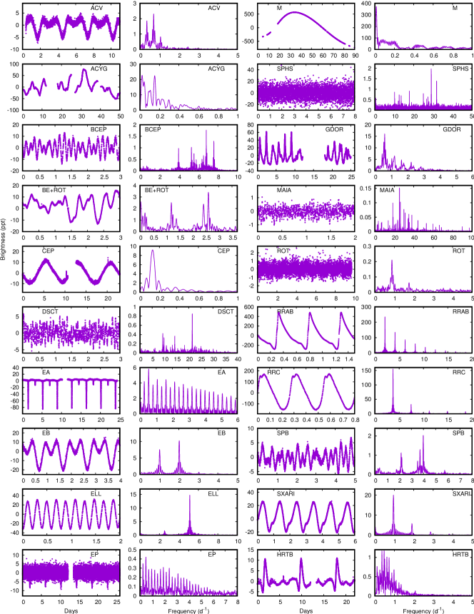
Figure 1: Examples of light curves and periodograms for different classes of variable stars observed by TESS. The brightness scale is parts per thousand.

4 The light curve and periodogram

The MAST website provides a bulk download script for all light curves in a particular TESS sector. The star number in this script is compared with the TIC number in the master catalogue. If there is a match, the light curve is downloaded as a FITS file. Typically, about 1000–4000 light curve files are downloaded per sector.

The next step is to extract the light curve from the FITS file to a text file. It is important to be able to generate the full path name of the light curve from the TIC number. The light curve of TIC 010510382, for example, is stored in file T010/010510382/010510382.dat. The text file contains three columns: the time (BJD), the simple aperture (SAP) light curve and the pre-search data conditioning (PDC) light curve in parts per thousand. If the star has previously been observed, the latest light curve is simply appended to the existing light curve. This procedure has been automated using suitable software.

The next step is calculation of the periodogram and extraction of significant frequencies, which is usually done by successive prewhitening. While this technique is perfectly adequate for ground-based light curves, problems arise when the signal-to-noise ratio, S/N, is very high, as it is in space photometry (Balona, 2014a). In addition, successive prewhitening is very slow and impractical for the task at hand.

This problem was solved by mapping the observed time series to a time series which is spaced by exactly 2 min, the spacing in the TESS observations. Where gaps exist in the time series, the data value is set to zero. This allows the periodogram to be calculated using the fast Fourier transform (FFT). For this purpose the number of data points needs to be a power of two. Normally, one would take the power of two just greater than the number of points in the time series and pad the excess with zeros. However, for greater resolution of the periodogram peaks, the time series was extended further by as much as a factor of 4 by zero padding. In this way one can obtained well-resolved periodograms of 1000–4000 stars in just a few hours. The periodogram is stored in the same folder as the light curve.

It is well known that the FFT is just another way of representing the data. It neither adds nor detracts from the information content. All frequencies which can be extracted are already visible in the FFT. These can be detected simply by noting the peaks in the FFT. This process is no different from trying to extract spectral line wavelengths in a crowded stellar spectrum. One picks the strongest lines, fits suitable curves to each line profile and removes them. Repeating the process one more time is sufficient to extract most of the remaining significant spectral wavelengths. The code which applies the FFT technique to the light curve also extracts the frequencies and amplitudes in the same way, the window function being used to model each peak.

As each frequency is extracted, the S/N ratio is calculated by measuring the amplitude relative to a smooth curve representing the periodogram background. The extracted information, which is stored in the same folder as the light curve and periodogram, contains the frequency, amplitude and their respective errors as well as the S/N. Peaks are deemed significant if S/N $>4.7$. After the periodogram for each star has been calculated, variability classification may begin. In this process, the periodogram plays a dominant role. In fact, in most cases it is not really possible to perform visual classification without the periodogram.

Before describing the next stage in the classification process, it is first necessary to discuss all the variability classes that were encountered.

5 Variability classes

Variability classification is a subjective process; the distinction between variability classes is often not clear unless strict guidelines are provided. The informal manner in which these classes were described for ground-based observations is no longer adequate in the age of space photometry.

For example, the $\gamma$ Dor class was originally defined as “F stars with multiple low frequencies”. This was perfectly adequate because the only F stars with multiple frequencies known at that time were the $\delta$ Sct stars. Since only high frequencies were observed in $\delta$ Sct stars (in agreement with the models), this definition of the $\gamma$ Dor stars presented no problem. The definition of “low frequencies” was typically taken as frequencies below about 5 d^-1 (approximately the lowest frequency observed in ground-based observations of $\delta$ Sct stars), but the exact value was not part of the definition. In order to drive low frequencies in $\gamma$ Dor stars, a different mechanism from that in $\delta$ Sct stars was required (Guzik et al., 2000), cementing the distinction between the two classes.

However, the distinction soon became blurred with the discovery of $\delta$ Sct+$\gamma$ Dor hybrids, i.e. $\delta$ Sct stars with both high and low frequencies (Handler et al., 2002). The few hybrids then known suggested that these were stars on the boundary between the two classes and could still be accommodated by theory. Later, when Kepler observations became available, it was found that practically all $\delta$ Sct stars contain low frequencies (Grigahcène et al., 2010).

The situation became even less clear when Gaia parallaxes became available. It was found that $\delta$ Sct stars occupy the same region of the H–R diagram as $\gamma$ Dor stars (Balona, 2018). It seems that $\gamma$ Dor stars are not a separate class after all. Under the circumstances, it is difficult to know whether one should perhaps rename the $\gamma$ Dor class in a way which unites it with the $\delta$ Sct class. Until a suitable model can be found to explain the low frequencies in $\delta$ Sct stars and how high frequencies are damped in $\gamma$ Dor stars, the problem will remain unresolved.

The same situation has recently been found in regard to the relationship between $\delta$ Sct and roAp stars. It turns out that many ostensibly non-peculiar stars pulsate with the high frequencies seen in roAp stars (above 60 d^-1). Furthermore, the fraction of $\delta$ Sct stars among Ap stars is no different from that in non-peculiar stars. Moreover, these $\delta$ Sct Ap stars have frequency peaks covering the whole frequency range. In other words, the roAp stars are just an arbitrary selection of Ap $\delta$ Sct stars with no particular significance (Balona, 2022a).

The significance perhaps lies in a subset of roAp stars in which equally-spaced multiplets, with spacing equal to the rotation frequency, are generated due to the effect of the strong magnetic field. This occurs at high frequencies when the pulsational wavelength is comparable to the atmospheric scale height. Perhaps it is more appropriate to restrict the name “roAp” to these stars. In any case, the class is probably too entrenched and we continue to use it for now to avoid confusion. The definition adopted here for roAp is any Ap star with frequencies in excess of 60 d^-1.

These high frequencies are also present in non-peculiar $\delta$ Sct stars where they were temporarily labeled “roA” stars by Balona (2022a), but this name is now dropped. Historically, the upper frequency limit for unstable modes in purely radiative models of $\delta$ Sct stars is about 50 d^-1. Here we label all $\delta$ Sct stars with independent frequencies higher than 50 d^-1 as DSCTH (i.e. $\delta$ Sct high frequency) and those with independent frequencies higher than 60 d^-1 DSCTU ($\delta$ Sct ultra-high frequency). An independent frequency is one which is not a linear combination of two lower frequencies or multiples of lower frequencies. Whether or not the subclasses DSCTH and DSCTU prove useful will have to be decided once we have a theory that can explain these pulsations.

Yet another example of the inadequacy of the current system was the realization that what appear to be $\gamma$ Dor stars are to be found at much higher effective temperatures than predicted by the models (Balona et al., 2016). These hot $\gamma$ Dor stars are to be found all along the upper main sequence and merge with what would be generally described as SPB stars (Balona & Ozuyar, 2020a). In order to avoid this confusion it is necessary to define an effective temperature which separates the two groups. This was taken to be $T_{\rm eff}=10\,000$ K in Balona & Ozuyar (2020a), a value that is continued in this paper.

Note that many stars are assigned more than one variability class. For example, a $\delta$ Sct star which is also suspected to show rotational peaks is classified as DSCT+ROT. The criterion used in pulsating stars with suspected rotational peaks is that the first harmonic must be clearly present and both peaks must be of reasonably high amplitude.

The notation SPB/BCEP means that the star may be either classified as an SPB or BCEP because it falls within the defined $T_{\rm eff}$ range for both stars, but the frequency peaks straddle the defined limits for both classes. In other words “+” means “and”; “/” means “or”.

A brief discussion of all variability classes used in this work now follows. Where there is a possibility of confusion with another class, the adopted limits on $T_{\rm eff}$ and frequency are given. This means that what is classified as a $\gamma$ Dor star may be re-classified as an SPB star, or vice-versa, if there is a change in the adopted $T_{\rm eff}$. Pictorial examples of what the light curves and periodograms might look like are shown in Fig. 1.

5.1 Dash

When a dash is allocated to a variability class it simply means that no significant variability was detected. It is also sometimes allocated to a star where there seems to be some indistinct, complex low-frequency variations which cannot be classified.

5.2 Pulsating variables

$\alpha$ Cyg (ACYG) Variables are supergiants with low frequencies which may be of pulsational origin or perhaps some other cause (Bowman et al., 2019). The light often shows smooth irregular variations, but may also be variable on shorter timescales. In the GCVS the designation is limited to B and A supergiants, but here we extend it to F supergiants as well.

$\beta$ Cep (BCEP) are pulsating O8–B6 main sequence stars with multiple periods in the range 0.1–0.6 d. The GCVS also defines a group of short-period $\beta$ Cep stars (BCEPS), but this class is obsolete. The long period end of this definition is more appropriate to SPB stars and in this work BCEP stars are limited to multiple frequencies in excess of 3 d^-1 and with $T_{\rm eff}>18000$ K (Balona & Ozuyar, 2020a). The class BCEPH denotes a BCEP with one or more frequencies higher than 50 d^-1.

The Maia variables (MAIA) are main sequence mid- to late B-type stars which pulsate in multiple high frequencies very similar to $\delta$ Sct stars (Balona et al., 2015, 2016). MAIAH and MAIAU are Maia variables with frequencies higher than 50 and 60 d^-1 respectively. The Maia stars merge with the $\beta$ Cep stars at high temperatures and with the $\delta$ Sct stars at lower temperatures. For this reason, the limit $10000<T_{\rm eff}<18000$ K was imposed to properly define the MAIA class. At low frequencies, Maia variables merge with the SPB stars. Therefore it is also necessary to impose a frequency limit of 5 d^-1. It has been suggested that Maia stars are just rapidly rotating SPB stars (Salmon et al., 2014), but this is not supported by $v\sin i$ measurements (Balona & Ozuyar, 2020a). The pulsations may be due to high degree modes (Daszyńska-Daszkiewicz et al., 2017).

In the GCVS the slowly pulsating B stars (SPB stars) are labeled as LPB (long-period pulsating B stars). In this paper we use the name SPB. These are multiperiodic mid- and late-B stars with frequencies less than about 5 d^-1. However, TESS has shown that these variables are present among all main-sequence B stars, including the hottest B stars (Balona & Ozuyar, 2020a). They can be confused with the $\beta$ Cep variables, many of which have frequencies as low as 3 d^-1. In order to avoid this confusion, the designation SPB is used for stars with $T_{\rm eff}>18000$ K with frequencies less than 3 d^-1. For cooler B stars ($10000<T_{\rm eff}<18000$ K), the frequency limit is extended to 5 d^-1 to avoid confusion with Maia variables (Balona & Ozuyar, 2020a). The SPB and $\gamma$ Dor stars seem to form a continuous sequence across all B, A and F main sequence stars for which no explanation exists at this time. For this reason, the SPB class is restricted to stars hotter than 10 000 K.

The $\gamma$ Dor stars (GDOR), $\delta$ Sct (DSCT) and roAp stars have already been discussed. To avoid confusion with $\delta$ Sct and SPB star, the frequencies in GDOR stars must be lower than 5 d^-1 and $T_{\rm eff}<10\,000$ K. The $\delta$ Sct stars must have $T_{\rm eff}<10\,000$ K to avoid confusion with Maia variables.

SX Phe (SXPHE) stars resemble the $\delta$ Sct variables but belong to spherical component or old disk galactic population. They are mainly present in globular clusters.

Solar-type oscillators (SOLR) are generally F or K stars with very low amplitude pulsations similar to the 5-min solar oscillations. Large numbers of these stars were detected by Kepler, but are much more difficult to identify with TESS owing to the larger noise level. The SOLR stars listed in this paper are all Kepler stars.

Cepheids (CEP) are F and G supergiants with radial pulsations. Later spectral types have longer periods. The GCVS has three other subclass, CEP(B), DCEP and DCEPS, but these are not used here.

The RR Lyraes (RR, RRAB, RRC) are radially pulsating Population II giants. They are present in large numbers in globular clusters. The general designation is RR, but most of the stars observed by Kepler and TESS are of the RRAB class with asymmetric light curves with a steep ascending branch. A few RRC stars, which have symmetrical almost sinusoidal light curves, have also been observed by TESS.

The W Vir stars (CW) are Population II pulsating variable). The subclasses CWA and CWB are W Vir stars with periods respectively longer and shorter than 8 d.

The RV Tau (RV) stars are radially pulsating supergiants with F/G spectral types at maximum and K/M at minimum with alternating primary and secondary minima. The minima vary in depth so that the primary minimum may become the secondary minimum and vice-versa. The period between two primary minima is 30–150 d. The subclass RVA does not vary in mean magnitude, while RVB does vary in mean magnitude.

The Mira (M) variables are long-period variable giants with characteristic late-type emission spectra (Me, Ce, Se) and semi-regular pulsations with periods 80–1000 d.

Semiregular variables (SR) are giants or supergiants of intermediate and late spectral types showing noticeable light periodicity (from 20 to over 2000 d), but with irregular interruptions. The GCVS divides these into subclasses SRA (persistent periodicity) and SRB (poorly defined periodicity). The SRD class are F, G or K supergiants with 30–1100 d periods.

In the GCVS the V361 Hya stars are labeled RPHS (rapidly pulsating hot subdwarfs), but there is no class for the slowly pulsating V1093 Her stars. The label SPHS is used here. The separation between the two classes is taken to be about 300 d^-1 in frequency, which means that it is not possible to detect pure RPHS stars with TESS. Those that are labeled RPHS are taken from the literature. Originally, there seemed to be a distinction in effective temperature between RPHS and SPHS stars, the SPHS being cooler. This distinction seems to have disappeared with further observations (Krzesinski & Balona, 2022). Most pulsating B subdwarfs appear to be hybrids (SPHS+RPHS).

PVTEL variables are helium supergiant Bp stars with weak hydrogen lines and enhanced lines of He and C. They pulsate with periods of approximately 0.1–1 d. The BLAP (blue large-amplitude pulsator) are a proposed new class of degenerate star (Pietrukowicz et al., 2013). At this stage little is known about them.

ZZ Ceti variables (ZZ) are nonradially pulsating white dwarfs with periods in the range 0.5–25 min. Flares are sometimes observed which are usually attributed to a cool companion. The ZZA are of DA spectral type, while ZZB are DB stars. The ZZO class was introduced in the GCVS for ZZ Cet variables of the DO spectral type showing HeII and and CIV absorption lines in their spectra. This also includes the GW Vir class.

5.3 Rotational variables

In the GCVS, the BY Dra (BY) variables are emission-line dwarfs of dKe-dMe spectral type showing quasi-periodic light changes with periods from a fraction of a day to 120 d. The light variability is caused by spots. Many such star also flare. The FK Com stars (FKCOM) are rapidly-rotating G or K giants with non-uniform surface brightness. The light variation is due to rotation.

In the GCVS the $\alpha^{2}$ CVn (ACV) stars are defined by a strictly periodic variation in B8p–A7p stars. They exhibit magnetic field and brightness changes (periods of 0.5–160 days or more). These peculiar main-sequence stars display strong lines of Si, Sr, Cr and rare earths. The light modulation is attributed to surface patches with differing abundances. In this work, the ACV designation is applied to any Ap/Fp star with $T_{\rm eff}<10000$ K which shows strict periodicity compatible with the expected rotation frequency.

In the GCVS, SX Ari (SXARI) variables are main sequence peculiar B stars with variable intensity He I and Si III lines and strong magnetic fields. The light period is the same as the rotational period. These are the high-temperature analogs of the ACV variables. In this paper, SX Ari stars are peculiar B stars with $T_{\rm eff}>10000$ K. We distinguish between the SX Ari stars and the He-weak and He-rich variables in that SXARI stars must have anomalous abundances of Si or Hg/Mn. This is a subject which requires a deeper study. The He-variable stars are usually classified as ROT if they have a strict light period consistent with rotation.

The label MRP describes stars which emit radio pulses, two per rotation period (Das et al., 2022). They appear to be ACV or SXARI stars.

Even a brief examination of Kepler or TESS photometry will show that a significant fraction of A and B stars have an isolated low frequency, low amplitude peak at less than 4 d^-1, consistent with what one might expect for the rotational frequency. The harmonic of the peak is often present. Many studies have shown that these are indeed to be identified as the rotational frequency (see Balona 2022b and references therein). The GCVS does not have a designation for hot stars with rotational modulation. For this reason, the ROT class was introduced. A subclass, the ROTD stars, is reserved for stars which show a sharp rotational peak at a slightly higher frequency than a broad peak which is suspected to be due to inertial modes (the “hump and spike” stars Balona 2014b; Saio et al. 2018). It is often not possible to distinguish between rotational modulation and low-level eclipses and for this reason the ROT class is restricted to frequency peaks with amplitudes less than 10 ppt. However, most of the ROT variables have amplitudes less than 0.5 ppt (Balona, 2022b).

5.4 Eclipsing variables

The general GCVS classification for eclipsing stars is E. However, more specific subclasses have been introduced. Note that not much attention has been payed to specific subclasses of eclipsing variables in this work. Generally, any star in which eclipses are suspected are classified as EA or EB.

The EA class, or Algol ($\beta$ Per)-class eclipsing systems, are binaries with spherical or slightly ellipsoidal components. This class is used when it is possible to specify the moments of the beginning and end of the eclipses. Between eclipses the light remains almost constant or varies insignificantly because of reflection effects.

The EB ($\beta$ Lyr) eclipsing systems have ellipsoidal components and light curves for which it is impossible to specify the exact times of onset and end of eclipses. The depth of secondary minimum is usually considerably smaller than that of the primary minimum.

AM Her variables (AM) are close binary systems consisting of a dK or dM star and a compact object with a strong magnetic field.

DM are detached main sequence binary systems in which the inner Roche lobes are not filled.

The HRTB (heartbeat stars, Welsh et al. 2011) are variable binary star systems in eccentric orbits with pulsations driven by tidal forces.

The ellipsoidal variables (ELL) are close binary systems with ellipsoidal components. The combined brightness varies with a period equal to the orbital period, but there are no eclipses.

In the GCVS the designation EP is given to stars with eclipses due to planets. In this work we use EP for any eclipse-like variation with an amplitude less than about 10 ppt. The periodogram typically contains several low-amplitude harmonics which could either be due to low-level eclipses or rotation. The distinction is made mainly on the number of visible harmonics. If only one or two harmonics are seen, then the star is classed as ROT, otherwise as EP. It is quite possible that many stars classified as EP are actually rotational variables or even planetary systems. An analysis of these stars for planetary systems would be interesting as very few A and B stars are known to host planets.

W UMa class eclipsing variables (EW) have periods shorter than 1 d and the primary and secondary minima are equal or almost equal in depth. In the GCVS this designation is used only for F or later type stars.

GS eclipsing systems are giants or supergiants where one of the components may be a main sequence star.

The RS CVn stars (RS) are eruptive variables in a binary system showing Ca II H and K emission. The light period is close to the orbital period and they are X-ray sources.

Table 5: A list of Kepler, K2 and TESS stars classified by the author. The full catalogue is available electronically. The column labeled p is the priority number for the adopted effective temperature. The rotation period, $P_{\rm rot}$ is given where applicable. The column marked pec is a code for the stellar peculiarity.

RA	Dec	Name	Var	$T_{\rm eff}$	$\log\tfrac{L}{L_{\odot}}$	p	$v\sin i$	$P_{\rm rot}$	pec	Sp. Type
279.8504662	-47.1368375	TIC 339907982	EB	31000	1.62	4			9	sdB,sdB,sdO/BsdB
279.8654723	25.1250158	TIC 316904504	-	7970	1.20	4				A0
279.8681614	45.3642605	TIC 383751023	-	7819	1.09	1			1	kA2hA6mF4
279.8695086	43.5142894	KIC 7797592	ROT	6905	0.83	3		1.326		[F5V]
279.8759807	-21.9655564	EPIC 216652481	ROT/SPB	12600	3.39	10	174.0	1.786	6	B8IIIe
279.8769148	-48.5085760	TIC 304451865	DSCT	7289	1.14	4				A8/9V
279.8783231	18.3319300	TIC 345978356	-	5971	0.11	6				G0
279.8834254	-55.3068028	TIC 120202126	ROT	6449	0.57	4		4.651		F3V
279.8867664	-72.9482134	TIC 344167219	-	6559	0.46	4				F3V
279.8876674	40.9350562	TIC 157696928	SPB	10423	2.51	1	106.0			B8:Vn + A0III

5.5 Eruptive and irregular variables

The designation FLARE is attached to any object where evidence of a flaring event is present in the light curve.

The Be stars (BE, BE+ROT) are eruptive B stars in which Balmer line emission is seen, though the emission might disappear and re-appear at different times. Recent observations from TESS have shown that about 75 percent of Be stars vary with short quasi-periods in the range 0.5–2.0 d (Balona & Ozuyar, 2020b). It is suggested that the eruptions and subsequent rotational modulation is a result of localized surface activity (flaring) which ejects material. This material is channelled to diametrically opposed regions where the geometric and magnetic equators intersect. The light and line-profile variation is due to obscuration by these trapped clouds which eventually disperse into the circumstellar disc (Balona & Ozuyar, 2021; Balona, 2022b).

Both the periodogram and the light curve are very distinctive. The periodogram normally shows a low-frequency group (suspected to be a result of circumstellar material) as well as two other groups. One group can be identified at about the expected rotational frequency, while the other group is at about twice the rotational frequency. This is a consequence of obscuration by the diametrically located trapped clouds. The amount of trapped material varies with time, sometimes resulting in the disappearance of the highest frequency group. What is clear is that the peaks are broad and vary in phase and amplitude with a timescale of weeks to months (Balona & Ozuyar, 2020b, 2021). The light curve often shows distinctive eclipse-like dips, quite different from the light curves of SPB and $\gamma$ Dor stars which vary in the same period range, but with strict coherent frequencies.

In this work, Be stars which show the three groups are labeled as BE+ROT while those which only show long-period variations are classed as BE. The ROT designation refers to the possible non-coherent rotational light variation of the two higher-frequency groups as described. The distinctive periodogram and light curve is sometimes seen in ostensibly non-Be stars. These may be incipient Be stars which are designated BEV or BEV+ROT.

The $\gamma$ Cas (GCAS) stars are Be stars with X-ray emission. The $\sigma^{2}$ Ori variables (SORI) are Be stars in which the light variation is due to circumstellar matter trapped by a strong tilted dipole magnetic field. Most Wolf-Rayet (WR) stars show irregular light variations, but periodicity is present in a few stars (WR+BCEP or WR+ROT).

UV are variables of the UV Ceti class, which are KVe–MVe stars sometimes displaying flare activity with amplitudes from several tenths of a magnitude up to several magnitudes.

The S Doradus (SDOR) are eruptive, high luminosity Bp–Fp stars showing irregular (sometimes cyclic) light changes with amplitudes 1–7 mag in V. As a rule, these stars are associated with diffuse nebulae and surrounded by expanding envelopes.

U Geminorum-class variables (UG), quite often called dwarf novae, are close binary systems consisting of a dwarf or subgiant K-M star that fills the volume of its inner Roche lobe and a white dwarf surrounded by an accretion disk. Orbital periods are in the range 0.05-0.5 d. These are divided into subclasses UGSU (SU UMa systems) and UGSS (SS Cyg systems) and UGZ (Z Cam systems).

Stars of variability class I are an homogeneous set of poorly studied irregular variables. This can be divided into class IA (early-type, O–A) and IB (late type). The IN type are irregular, eruptive variables connected with bright or dark diffuse nebulae or observed in the regions of these nebulae. These again are divided into early type (INA) and late type (INB). The INS and ISA classes show rapid light variations. INT or IT are Orion variables of the T Tauri type. NL are poorly studied eruptive nova-like variables. PN stars are the nuclei of planetary nebulae. The LB class describes late-type stars with slow irregular variations.

The NB, NC and NL classes are novae with fast (NA), slow (NB) and very slow (NC) light variations. The NL class are poorly studied nova-like variables.

XP denotes an X-ray pulsar source. The subclass XNG describes a nova-like transient system consisting an early-type giant or supergiant with a compact companion.

6 Classification

Once the TESS stars have been downloaded and the periodograms calculated, the next step is to display the light curves and periodograms of unclassified stars for visual classification. It is imperative that these curves be displayed with the utmost ease to reduce the time required for classification. For this purpose, software was developed which enabled the display of these curves by simply clicking on a list of TIC star numbers.

The periodogram is the most important source of information for classifying purposes. The process requires two passes. In the first pass, the full frequency range of the periodogram is displayed (0–360 d^-1) so that high frequencies can be detected. In this pass, many $\delta$ Sct stars and eclipsing binaries are normally seen. In the second pass, the displayed frequency range is narrowed to 0–10 d^-1. This pass proceeds more slowly as other classes of variable are identified. In every new TESS release there are around 1000–2000 previously unclassified stars. The process of classification is usually accomplished in 2–4 days.

Among the stars in the master catalogue observed by Kepler, K2 and TESS, only about 2 percent appear in the GCVS. The variability class derived by visual inspection is nearly always in good agreement with the GCVS class, but corrections were sometimes made.

An extract of the catalog, which is complete up to TESS sector 55, is shown in Table 5. In this table, stars without spectral type have been assigned spectral types in accordance with the measured $T_{\rm eff}$ and $\log L/L_{\odot}$. These spectral types are enclosed in square brackets. The stellar peculiarity has been assigned a code in accordance with the following scheme: 1: Am (CP1); 2: Ap (CP2); 3: Hg/Mn (CP3); 4: He-weak (CP4); 5: He-rich (CP5); 6: Classical Be; 7: Herbig Be; 8: $\lambda$ Boo; 9: sdOB.

There are 20 744 stars observed by Kepler, 5 877 stars observed by K2 and 94 186 TESS stars (total 120 807 stars). The location of several types of pulsating star in the H-R diagram is shown in Fig. 2.

Figure 2: Location of some pulsating stars in the H–R diagram. The solid line is the zero-age main sequence from solar composition models by Bertelli et al. (2009).

Table 6: Number of stars in the most common classes and sub-classes.

Class	N	Class	N
TOTAL	120807	FLARE (all)	1146
Non-variable (-)	45064	Be (all)	723
		BE+ROT	589
Rotational (all)	42983	SORI	15
ROT	1302	BEV	49
ROTD	289	GCAS	3
BY	8
FKCOM	2	BCEP (all)	700
ACV	996
SXARI	675	Maia (all)	518
		MAIA	475
$\delta$ Sct (all)	13755	MAIAH	28
DSCT	10164	MAIAU	15
DSCTH	1468
DSCTU	2001	ACYG (all)	426
ROAP	121
		Tidal (all)	459
GDOR (all)	6128	ELL	374
		HRTB	85
Eclipsing (all):	5928
EA	2722	SPHS	178
EB	1996
EP	970	CEP	132
EW	216	CW	16
SOLR (all)	2415	RRAB	198
SPB (all)	1286	RRC	52

7 Conclusions

Over the last decade, the author has been visually classifying the light variations of stars observed by Kepler, K2 and TESS. The classification system has been kept as close as possible to that of the General Catalogue of Variable Stars, but a few modifications were inevitable. The results are presented as a table of over 120 000 stars. These data could be used as a learning sample for an artificial intelligence code which can then be applied to all TESS light curves. Table 6 summarizes the number of stars in each class and subclass for the most common classes.

The informal and rather vague definitions of variability classes in the General Catalogue of Variable Stars is no longer appropriate to the large number of stars observed from space photometry. In this work we have attempted to define the classes according to limits of effective temperature and frequency, where necessary. There is a pressing need for a more comprehensive theoretical understanding of stellar pulsation along the main sequence. It is quite clear that preconceived assumptions regarding the atmospheres in upper main sequence stars need to be relaxed. Until the models are able to replicate the locations of the stars in the H–R diagram and their pulsational frequencies, no progress can be made in understanding the different classes of pulsational variables that have been observed.

In order to support this project, the author has also been collecting estimates of effective temperature from the literature. This is presented as a table of over 900 000 individual measurements for nearly 635 000 stars with literature references and a code which indicates the method used. A catalogue of projected rotational velocities containing over 75 000 individual measurements for nearly 52 000 stars with bibliographic reference code is also presented.

The assigned variability class represents the author’s opinion and it is possible that others would assign a different class for many stars. There is no “correct” variability class. There are, no doubt, errors in these three catalogues which have escaped the author’s attention and there is no claim of completeness in any of these catalogues. They are presented in the hope that they will prove useful to the community.

Data availability

All data are incorporated into the article and its online supplementary material. The data are available at:

https://sites.google.com/view/tessvariables/home

References

- Anders et al. (2022) Anders F., Khalatyan A., Queiroz A. B. A., et al., 2022, A&A, 658, A91
- Audenaert et al. (2021) Audenaert J., Kuszlewicz J. S., Handberg R., et al., 2021, AJ, 162, 209
- Balona (2014a) Balona L. A., 2014a, MNRAS, 439, 3453
- Balona (2014b) —, 2014b, MNRAS, 441, 3543
- Balona (2018) —, 2018, MNRAS, 479, 183
- Balona (2022a) —, 2022a, MNRAS, 510, 5743
- Balona (2022b) —, 2022b, MNRAS, 516, 3641
- Balona et al. (2015) Balona L. A., Baran A. S., Daszyńska-Daszkiewicz J., De Cat P., 2015, MNRAS, 451, 1445
- Balona et al. (2016) Balona L. A., Engelbrecht C. A., Joshi Y. C., et al., 2016, MNRAS, 460, 1318
- Balona & Ozuyar (2020a) Balona L. A., Ozuyar D., 2020a, MNRAS, 493, 5871
- Balona & Ozuyar (2020b) —, 2020b, MNRAS, 493, 2528
- Balona & Ozuyar (2021) —, 2021, ApJ, 921, 5
- Bertelli et al. (2009) Bertelli G., Nasi E., Girardi L., Marigo P., 2009, A&A, 508, 355
- Blomme et al. (2010) Blomme J., Debosscher J., De Ridder J., et al., 2010, ApJ, 713, L204
- Blomme et al. (2011) Blomme J., Sarro L. M., O’Donovan F. T., et al., 2011, MNRAS, 418, 96
- Bowman et al. (2019) Bowman D. M., Burssens S., Pedersen M. G., et al., 2019, Nature Astronomy, 3, 760
- Brown et al. (2011) Brown T. M., Latham D. W., Everett M. E., Esquerdo G. A., 2011, AJ, 142, 112
- Chen et al. (2019) Chen Y., Girardi L., Fu X., et al., 2019, A&A, 632, A105
- Das et al. (2022) Das B., Chandra P., Shultz M. E., et al., 2022, ApJ, 925, 125
- Daszyńska-Daszkiewicz et al. (2017) Daszyńska-Daszkiewicz J., Walczak P., Pamyatnykh A., 2017, in European Physical Journal Web of Conferences, Vol. 160, European Physical Journal Web of Conferences, p. 03013
- Gaia Collaboration et al. (2022) Gaia Collaboration, Gaia Collaboration, De Ridder J., et al., 2022, arXiv e-prints, arXiv:2206.06075
- Gaia Collaboration et al. (2016) Gaia Collaboration, Prusti T., de Bruijne J. H. J., et al., 2016, A&A, 595, A1
- Glebocki & Gnacinski (2005) Glebocki R., Gnacinski P., 2005, VizieR Online Data Catalog, 3244
- Gontcharov (2017) Gontcharov G. A., 2017, Astronomy Letters, 43, 472
- Green et al. (2019) Green G. M., Schlafly E., Zucker C., Speagle J. S., Finkbeiner D., 2019, ApJ, 887, 93
- Grigahcène et al. (2010) Grigahcène A., Antoci V., Balona L., et al., 2010, ApJ, 713, L192
- Guzik et al. (2000) Guzik J. A., Kaye A. B., Bradley P. A., Cox A. N., Neuforge C., 2000, ApJ, 542, L57
- Handler et al. (2002) Handler G., Balona L. A., Shobbrook R. R., et al., 2002, MNRAS, 333, 262
- Krzesinski & Balona (2022) Krzesinski J., Balona L. A., 2022, A&A, 663, A45
- Pietrukowicz et al. (2013) Pietrukowicz P., Dziembowski W. A., Mróz P., et al., 2013, Acta Astron., 63, 379
- Pojmanski et al. (2005) Pojmanski G., Pilecki B., Szczygiel D., 2005, Acta Astron., 55, 275
- Saio et al. (2018) Saio H., Kurtz D. W., Murphy S. J., Antoci V. L., Lee U., 2018, MNRAS, 474, 2774
- Salmon et al. (2014) Salmon S. J. A. J., Montalbán J., Reese D. R., Dupret M.-A., Eggenberger P., 2014, A&A, 569, A18
- Samus et al. (2017) Samus N. N., Kazarovets E. V., Durlevich O. V., Kireeva N. N., Pastukhova E. N., 2017, Astronomy Reports, 61, 80
- Skiff (2014) Skiff B. A., 2014, VizieR Online Data Catalog, 1, 2023
- Soubiran et al. (2016) Soubiran C., Le Campion J.-F., Brouillet N., Chemin L., 2016, A&A, 591, A118
- Stassun et al. (2018) Stassun K. G., Oelkers R. J., Pepper J., et al., 2018, AJ, 156, 102
- Welsh et al. (2011) Welsh W. F., Orosz J. A., Aerts C., et al., 2011, ApJS, 197, 4
- Wenger et al. (2000) Wenger M., Ochsenbein F., Egret D., et al., 2000, A&AS, 143, 9