Modelling the CO streamers in the explosive ejection of Orion BN/KL region

Abstract

We present reactive gasdynamic, axisymmetric simulations of dense, high velocity clumps for modelling the CO streamers observed in Orion BN/KL. We have considered 15 chemical species, a cooling function for atomic and molecular gas, and heating through cosmic rays. Our numerical simulations explore different ejection velocities, interstellar medium density configurations, and CO content. Using the CO density and temperature, we have calculated the CO ($J=2\to 1$) emissivity, and have built CO maps and spatially resolved line profiles, allowing us to see the CO emitting regions of the streamers and to obtain position velocity diagrams to compare with observations. We find that in order to reproduce the images and line profiles of the BN/KL CO streamers and H₂ fingers, we need to have clumps that first travel within a dense cloud core, and then emerge into a lower-density environment.

1 Introduction

Currently, the star formation paradigm considers that isolated pre-stellar cores evolve through accretion to become a star. In the case of low-mass stars, there is enough evidence to classify them from early to late protostars and their duration in the Class 0 through Class III objects. More massive forming stars seem to undergo a similar process, nevertheless, they are formed in dense environments which could produce close dynamical encounters that may even interrupt the accretion process. This effect has been recently invoked as the origin of explosive outflows, which have been reported to have occurred in at least three massive star-forming regions (Zapata et al., 2011, 2013, 2017, 2020). The closest of these explosive outflows is the Orion BN/KL region, located behind the Orion Nebula (at a distance of 414 pc from the Sun; Menten et al., 2007). The most accepted qualitative model for this object (Bally et al., 2005) proposes that a single ejection event could have been caused by a stellar merger or the dynamic rearrangement of a non-hierarchical system of young, massive stars or protostars and, more quantitatively, now there is an active effort to explain the formation of these explosive outflows (Tan, 2004; Zapata et al., 2009; Goddi et al. 2011, ; Bally et al., 2011; Raga et al., 2021; Rivera-Ortiz et al., 2021).

The Orion BN/KL region has three dynamical components: a breaking-up multiple stellar systems, an expanding molecular bubble, and a peculiar outflow with about 200 filamentary structures, detected in H₂ and in CO ($J=2\to$1), known as “fingers” and “streamers”, respectively. All components seem to have originated in the same event approximately 500 yr ago (Zapata et al., 2009). The fingers are the more extended and the first to be discovered. The Orion fingers were reported by (1993) as H₂ 2.1$\mu$m features emanating outwards from the central region of Orion BN/KL and terminating in a series of Herbig-Haro (HH) objects, which had previously been observed as [O I] 6300, high-speed “bullets” by Axon & Taylor (1984). These HH objects have been detected in other optical lines (O’Dell, 1997). The kinematics of the H₂ emission features has been studied with Fabry-Perot observations (Chrysostomou et al., 1997; Salas et al., 1999) and proper motion measurements Bally et al. (2011). The proper motions of some of the optically detected bullets have also been presented by Doi et al. (2002).

Following Bally et al. (2011 and 2015) there are about 200 H₂ fingers, which present a distribution of longer features to the NW, shorter fingers to the SE and SW, and very few and weak features to the E and NE. The longer fingers have a length of $\sim 50000$ au (using the distance of 414 pc) and diameters between 800 to 3200 au. The shorter filaments are narrower, more numerous, and tend to overlap. The heads of the H₂ fingers (seen in H₂ and [Fe II] IR lines and optically as HH objects, see above) have diameters $\sim 40\to 400$ au. The well-defined, longer filaments have velocities (derived from the radial velocity and proper motion measurements) of $\sim 350$ km s^-1. The lengths and velocities of the fingers are consistent with an origin in a single ejection event (for all fingers) $\sim 500\to 1000$ yr ago. However, there is evidence of substantial braking of the motion of the heads of those fingers over their evolution (Bally et al., 2011). An estimation of the total kinetic energy of the fingers is about $10^{47}\to 10^{48}$ erg, which can be interpreted as an estimation of the energy of an “ejection event” that gave rise to the present-day fingers (Bally et al., 2011).

This region also has an extended CO outflow which was first detected in single-dish observations by (Kwan & Scoville, 1976). In more recent interferometric observations, this outflow has been resolved into a system of CO “streamers” (Zapata et al., 2009; Bally et al., 2017). The streamers show a more isotropic direction distribution than the H₂ fingers, with several streamers travelling to the NW emitting in the CO $J=2\to$1 rotational transition. The total mass moving with velocities larger than 20 km s^-1 is $\sim 8$ M_⊙ (Bally et al., 2015, and references therein). In order to propose a mean mass in each of the fingers, one can assume that all fingers have the same mass, therefore dividing total mass in this region by the $\sim 200$ observed fingers obtaining mass per finger of $\sim 0.04$ M_⊙ (Rivera-Ortiz et al., 2019).

Many of the CO streamers partially coincide with the H₂ fingers but they do not reach out to the position of the optical “bullets” at the tip of the fingers. Typically, the CO emission of the streamers fades away at a fraction $\epsilon=0.3\to 0.7$ of the length of the corresponding H₂ fingers. The CO streamers are barely resolved with the ALMA interferometer, with widths of $400\to 800$ au (Bally et al., 2017). Therefore, the CO streamers are shorter and narrower than the H₂ fingers by a factor of $\sim 2$. As some of the fingers and the streamers are spatially coincident and have different widths, it can be argued that the CO emission is produced inside the H₂ fingers.

The radial velocities show a quite dramatic pattern of mostly red-shifted CO streamers to the W and SW, blue shifted streamers to the N and E, and intermixed blue- and red-shifted streamers to the NW. Also, the CO streamers have “Hubble law”, linear radial velocity vs. distance signatures, which are also in good agreement with a simultaneous ejection $\sim 500$ yr ago (see Zapata et al., 2009). These “Hubble law” velocity vs. distance signatures indicate that the CO emitting material has not suffered substantial braking. The peak radial velocities (at the tip of the CO streamers) have values of less than $\sim 120$ km s^-1, corresponding to approximately 1/2 of the fastest spatial motions of the H₂ fingers (of $\sim 350$ km s^-1, see above). However, it has been challenging to note that even when Orion H₂ fingers are larger than the CO streamers, they have different kinematic ages and do not follow a Hubble law. This could be explained by taking into account the interaction between the environment and the leading clumps that generate the fingers. Rivera-Ortiz et al. (2019) used a dynamical model based on a plasmon equation of motion (DeYoung and Axford 1967 and Rivera-Ortiz et al. 2019) to explain the age discrepancy and obtained an inferior limit for their ejection conditions.

The environment that surrounds the Orion BN/KL outflow is a dense molecular core. Oh et al. (2016) set a lower density of $10^{5}$ cm^-3, analyzing the extinction and the overall angular spread of the H₂ emission. From the CO emission, Bally et al. (2017) found an environment density between $10^{6}$ and $10^{7}$ cm^-3, assuming a $X_{CO}=10^{-4}$ CO fraction and a background temperature of 10 K. Lower values of $X_{CO}$ would lead to higher estimates of the environmental density.

The connection between the H₂ fingers and the CO streamers seems to be direct, both being created by leading bullets. Nevertheless, their differences need to be modelled and understood in order to explain and interpret the observations of similar explosive outflows, which are detected at high resolution with ALMA in the CO J=$2\to 1$ line but not in H₂ emission, such as DR21 and G5.89, which are at larger distances from us.

This paper presents simulations of the CO streamers in the Orion BN/KL region. In our models, the streamers are produced by fast clumps travelling within a structured environment. In particular, we study the effects of having a central, “dense cloud” environment, from which the clumps emerge into a lower-density medium. This configuration has been shown to lead to the production of linear ramps in the predicted position-velocity diagrams from the resulting flows (Raga et al., 2022). Notice that we deal with CO emission and compare the kinematic properties obtained from the numerical models with the observations. A larger study is necessary in order to better conciliate the CO and H2 emission, simultaneously.

The paper is organized as follows: in Section 2 we present the numerical setup of the simulations. In section 3, we present the results of the CO emission analysis. Finally, the contribution of these models to our understanding of the Orion BN/KL region is discussed in section 4.

2 Numerical simulations

We have computed 2D numerical simulations using Walkimya-2D. The code solves the hydrodynamic equations (Esquivel et al. 2009) and a chemical networks on an axisymmetric grid, The code is described in detail by Castellanos-Ramírez et al. (2018) and Rivera-Ortiz et al. (2022). The chemical network tracks the abundances of 15 chemical species: non-equilibrium evolution of C, C₂, CH, CH₂, CO₂, HCO, H₂O, O, O₂, H⁺, H^-, H and via conservation laws H₂, CO and OH are calculated. The selection of this network of species and the involved reactions is such that they can explain the CO abundances in other astrophysical situations (Castellanos-Ramírez et al. 2018).

The complete set of equations for a reactive flow are presented in Castellanos-Ramírez et al. (2018) and references therein. For a 2D flow, the reactive flow equations can be written as:

$$\frac{\partial\mathbf{U}}{\partial t}+\frac{\partial\mathbf{F}}{\partial x}+\frac{\partial\mathbf{G}}{\partial y}=\mathbf{S},$$ (1)

where $(x,y)$ are the (axial, radial) coordinates of the cylindrical domain, the vector $\mathbf{U}$ contains the so-called conservative variables, $\mathbf{F}$ and $\mathbf{G}$ are the fluxes in the $x$ and $y$-directions (respectively) and $\mathbf{S}$ is the sources vector. $\mathbf{S}$ contains the geometric terms resulting from the cylindrical grid geometry, energy gain/loss terms (in the energy equation) and molecular formation/destruction rates (in the continuity equations for the different chemical species). We, therefore, calculate the reaction rates for each of the chemical species and include the thermal energy gain and loss due to interaction with the radiative field or associated with the latent heat of the chemical reactions and/or the internal energy of the molecular, atomic or ionic species.

The energy equation includes the cooling function described by Raga & Reipurth (2004) for atomic gas and for lower temperatures we have included the parametric molecular cooling presented by Kosińsky & Hanasz (2007),

$$\Lambda_{\rm mol}(T)=L_{1}\cdot T^{\epsilon_{1}}+L_{2}\cdot\exp\left(-\frac{c_{*}}{(T-T_{*})^{\epsilon_{2}}}\right)\;\;,$$ (2)

for a temperature $T<5280$ K, where, $L_{1}=4.4\times 10^{-67}$, $L_{2}=4.89\times 10^{-25}$, $c_{*}=3.18$, $\epsilon_{1}=10.73$, $\epsilon_{2}=0.1$ and $T_{*}=1.0$ K. The total radiative energy for temperatures lower than 5280 K is given by $L_{rad,mol}=n_{\rm gas}\cdot n_{\rm CO}\cdot\Lambda_{\rm mol}(T)$, where $n_{\rm gas}$ and $n_{\rm CO}$ are the numerical densities of the gas and the CO molecule, respectively. The cosmic ray ionization rate of atomic hydrogen is $\Gamma_{\rm crp}=5\times 10^{-28}n_{\rm H}$, see Henney et al. (2009).

Finally, the thermal pressure is given by $P=(n+n_{e})kT\,,$ where $n$ is the total density of molecules+atoms+ions, $n_{e}$ is the electron density and and k is the Boltzmann constant.

Bally et al. (2015) modeled a “CO streamer” as the wake left behind by a fast, dense clump moving in a uniform environment. In the present paper, we study the case of a clump moving in an environment with a transition from an inner, dense region to an outer, lower-density region. Our simulations follow the dynamics of a clump that is initially moving inside a dense core of density $n_{cl}$ and temperature $T_{cl}$ and then emerges into a homogeneous medium with number density n_a and temperature $T_{a}$. The CO compositions of the high velocity clump, the cloud core and the external environment and of the external environment are also considered as free parameters (see Figure 1).

The simulations are done on a binary adaptative mesh with 7 refinement levels, yielding a maximum resolution of $4096\times 1024$ (axial $\times$ radial) cells, in a computational domain of $48000\times 12000$ au. Therefore, the maximum resolution of the simulation is 11 au per pixel. We used reflective boundary conditions for the symmetry axis and a free outflow boundary condition for all the other frontiers. The size of the mesh is large enough so that the choice of outer boundaries does not affect the simulation.

For the initially spherical and homogeneous, fast clump, we choose:

• a velocity $v_{c}=300\to 500$ km s^-1,

• a radius $r_{c}=50$ au (in the range of sizes observed for the heads of the H₂ fingers),

• a mass $M_{c}=0.01$ M_⊙, resulting in an initial number density of H₂ molecules $n_{c}=10^{10}$ cm^-3,

• a temperature $T_{c}=30$ K.

These parameters are consistent with the H₂ and CO observations of the finger/stream system discussed above.

Figure 1 shows a schematic diagram of the components in the simulation: The initial fast clump of radius $R_{cl}$ moving at a velocity $v_{cl}$, with density $n_{cl}$, temperature $T_{cl}$, and molecular fraction $\chi_{cl}$. The clump is immersed in a static cloud of radius $R_{c}$, density $n_{c}$, at temperature $T_{c}$ and with a molecular fraction $\chi_{c}$. Finally, the density, temperature and molecular fraction of the external medium are $n_{a}$, $T_{a}$ and $\chi_{a}$, respectively.

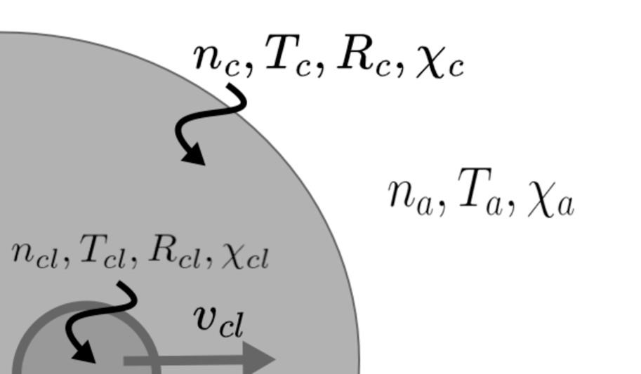
Figure 1: Schematic diagram showing the initial condition of the simulations. A fast clump initially travels within a dense cloud (of density $n_{c}$) and later emerges into a lower density, homogeneous environment (of density $n_{a}$).

In all runs, we assumed that the chemical composition of the interstellar medium is a free parameter. We have run 7 numerical simulations using different initial values of the density of the clump and initial CO compositions for each of the phases.

The fast clump travels along the $x$-axis, and is initially located at 500 au from the left boundary of the computational grid. It has an initial radius of 50 au, and has a $\rm CO$ abundance of 1.67$\times 10^{-4}$ with respect to $\rm H_{2}$. The total gas density is given by adding the individual H₂, H, CO, C and O densities, or by adding the densities of atomic and molecular gas. The clump has an initial temperature of 30 K and a 0.03 M_⊙ mass.

In all the models we have considered an external environment of density $n_{a}=10^{5}$ cm^-3 cm^-3 and temperature $T_{a}=1000$ K. We have included a central, dense core with a radius of $R_{c}=2000$ au, density $n_{c}=100\,n_{a}$ and in pressure equilibrium with the ambient medium.

The three components (high-velocity clump, central cloud, and outer environment) are present in all models except M0 and M00. In these two simulations, the clump travels within a homogeneous environment of density $n_{a}$, and the dense, central cloud is absent. Table 1 gives the molecular fraction of the three initial components of the simulations.

Table 1: Chemical initial conditions of the numerical simulations

Model	$\chi_{a}$	$\chi_{c}$	$\chi_{cl}$
M00	0	$--$	0.99
M0	0.99	$--$	0.99
M1	0.99	0.99	0.99
M2	0.99	0.99	0
M3	0	0	0.99
M4	0	0.99	0
M5	0.1	0.99	0.1

2.1 The CO emissivity

We expect to have strong CO emission arising, mainly, from the three zones: a) the high-velocity clump, b) the tail formed by the material left behind by the clump, and c) the environmental gas shocked by the wings of the bow shock around the clump. The simulations show that a substantial amount of material is dragged out of the central, dense cloud (within which begins the motion of the fast clump) as a result of the passage of the clump bow shock. This process is fundamental in determining the CO emission of the wake left behind by the fast clump.

To calculate CO emission maps and position-velocity diagrams that can be compared with observations, we calculated the CO $J=2\to 1$ emission coefficient in each of the computational cells using the CO density and the temperature of the gas as

$${j_{\rm{2\to 1}}}=\frac{1}{4\pi}\frac{g_{1}}{g_{2}}n_{\rm CO}\cdot e^{\frac{-E_{\rm{2\to 1}}}{kT_{{2\to 1}}}}A_{\rm{2\to 1}}E_{\rm{2\to 1}},\\$$ (3)

where, $g_{1}=3$ is a degeneracy factor, $Z(T)=\sum^{N}_{i}e^{-T_{\rm levCO}/T(i,j)}$ is the partition function, with $T_{\rm levCO}$ as the temperature of the corresponding energy levels, $A_{{2\to 1}}=7.16\times 10^{-7}$ s^-1 is the spontaneous emission coefficient, $E_{{2\to 1}}=h\nu_{{2\to 1}}$ is the energy of the transition with, $\nu_{{2\to 1}}=230.538$ GHz and $h$ is the Planck constant (Rybicki & Lightman, 1986).The emission maps and position-velocity diagrams are obtained through appropriate integrals of the emission coefficient along the lines of sight.

2.2 CO maps and position-velocity diagrams

Using the emission coefficients, we have constructed CO emission maps and position-velocity (PV) diagrams to compare our numerical results with the observational data presented in the literature.

First, we have computed CO ($J=2\to 1$) emission maps by appropriately rotating and integrating the axisymmetric simulations. All of the CO maps discussed below we have considered a $\phi=0$ orientation angle, corresponding to an outflow axis on the plane of the sky.

We have also calculated spatially resolved line profiles, considering the radial velocity and thermal Doppler profiles for the emission of the computational cells. With these line profiles, we then computed PV diagrams, integrating the emission perpendicularly to the projected outflow axis. The PV diagrams discussed below have been computed for different values of the orientation $\phi$ between the outflow axis and the plane of the sky.

For the CO emission maps and PV diagrams, we have not included the CO emission of the gas with absolute velocities lower than 3 km/s. This is to avoid contaminating our results with the CO emission coming from the unperturbed environment. This velocity cutoff is similar to the one used by Zapata et al. (2009) for presenting the CO emission of the Orion fingers.

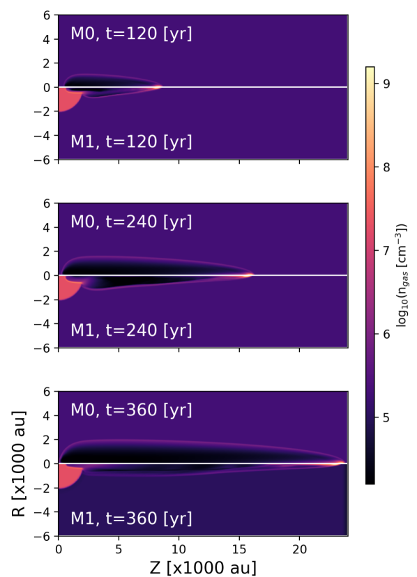
Figure 2: Density stratifications obtained for models M0 (bottom half of each plot), and M1 (top half) at times $t=$ $120$ (top), $240$ (centre) and $360$ yr (bottom). In model M1, the fast clump emerges from a central, dense cloud (which is not present in model M0). The logarithmic colour scale is shown by the bar on the right, and the axial and radial axes are labelled in units of $10^{3}$ au.

Finally, our emission maps and PV diagrams were convolved with a spatial gaussian profile with FWHM) corresponding to the synthetic beamsize of the ALMA interferometer of $1\arcsec$ (corresponding to 400 au at the distance of Orion).

3 Results

We first discuss the results obtained for the M0 and M1 models, which have the same initial chemical distribution (with molecular gas in all of the initial computational domain). These two models differ in that model M1 has a central dense cloud, and model M0 does not.

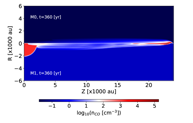
Figure 3: CO density stratifications obtained from Models M0 and M1 (upper and lower panel, respectively) for an evolutionary time of 360 yr. One can see that the highest density of CO is found in the clump, in the shocked ISM, in a small tail behind the clump and in a flow of material from the central cloud (for Model M1) that injects low-density material that produces the expansion of shock waves.

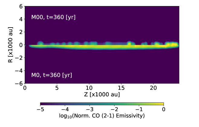
Figure 4: The CO integrated emissivity, on the plane of the sky, for Models M0 and M00 (top and bottom panels, respectively), at an evolutionary time of 360 yr.

Figure 2 shows the numerical density stratifications of models M0 and M1 (upper and bottom panels, respectively) at evolutionary times of 120, 240, and 360 yr (top, middle and bottom panels, respectively). In all of the time frames, we see that the clump of model M0 at all times:

• has a position that slightly trails behind the position of the M1 clump,

• has a smaller radius,

• has a radially more confined bow shock and wake region,

These are the three qualitative results of the passage through the central, dense cloud present in the initial flow configuration in model M1 (but absent in model M0).

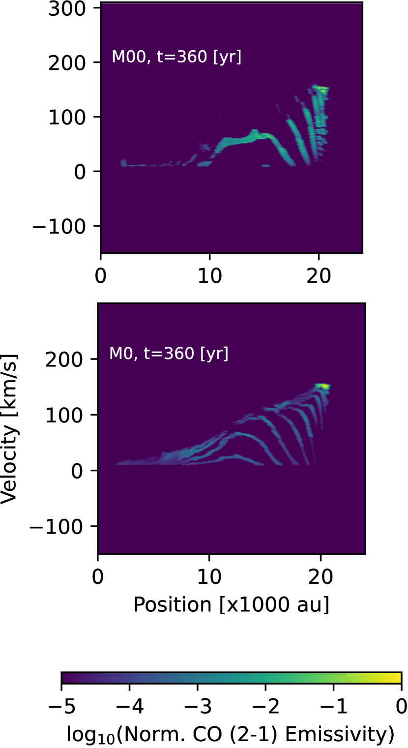
Figure 5: Position-velocity (PV) diagrams obtained from models M00 (top) and M0 (bottom) for a $t=360$ yr evolutionary time assuming a $\phi$ = 30^∘ angle between the outflow axis and the plane of the sky. The PV diagrams are normalized to the peak emission of each frame, and are shown with the logarithmic colour scale given by the bottom bar. The radial velocity is labeled in km s^-1 and the axial coordinate in $10^{3}$au

Figure 3 shows the CO density stratification for models M0 and M1 at t=360 yr. the density structure is very different for these two models, as expected. At M0 the highest molecular content is found mainly in the leading clump, that was originally blown, and a CO plume is visible (mainly) in the shocked gas region. And for model M1, it can be observed (as well as gas density) a stream of CO coming out from the central cloud inserted in the empty region behind the clump, and the fingertip does not have the maximum CO density of the model. This maximum is found in the central cloud and in the steam coming from there because of the pressure gradient between the cloud and the internal region of the bow shock that produces a vacuum.

Figure 4 shows CO ($J=2\to 1$) emission maps obtained from models M00 and M0 (top and bottom panels, respectively) at a $t=360$ yr evolutionary time, assuming that the outflow axis lies on the plane of the sky. For model M00 (which has a fast, molecular clump moving in a uniform atomic environment, see Table 1), the CO emission comes from the fast clump, and from detrained clump material which has been left behind in the wake of the clump, that is, material that has been entrained from the central core by the clump, that eventually slows down, filling the wake. For model M0 (with a molecular clump moving in a uniform molecular environment, see Table 1) the CO emission also has a strong contribution from environmental material shocked by the wings of the bow shock around the fast clump.

In Figure 5, we present the PV diagrams (showing the line profiles integrated across the outflow axis, as a function of position along this axis) obtained from models M00 and M0 (top and bottom panels, respectively), assuming an angle of $30^{\circ}$ between the outflow direction and the plane of the sky, for a $t=360$ yr evolutionary time.

In these PV diagrams, the peak emission comes from the fast clump itself. The region between the clump and the outflow source is occupied by a series of arcs (in the PV plane), produced by the detrained clump material in the wake of the clump. The emission within this region has an upper envelope of increasing peak radial velocity as one moves away from the outflow source. These models do not produce the linear velocity vs. position ramp observed in the Orion fingers (see, e.g., Zapata et al. (2009)).

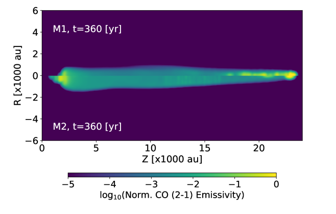
Figure 6: The CO for Models M1 and M2 (top and bottom half, respectively), at a $t=360$ yr evolutionary time, computed assuming that the outflow axis lies on the plane of the sky. The emission (shown with the logarithmic colour scale given by the bottom bar) is normalized to the peak intensity in each of the maps. The plane of the sky coordinates is in units of $10^{3}$au.

We now present CO $J=2-1$ intensity maps and PV diagrams from models M2-M5, in all of which the fast clump first travels through a central, dense cloud and then emerges into a lower-density, uniform environment. Figure 6 shows the CO emission maps (assuming that the outflow axis is on the plane of the sky) for models M1 and M2, at $t=360$ yr (top and bottom panels, respectively). In these models (unlike the models that do not have a central cloud, see Figure 4), the CO emission fills the cavity behind the clump bow shock, and has the peak emission in the region in which the flow emerges from the dense cloud. In model M1 (in which all of the initial components are molecular, see Table 1), a peak in the CO emission is also observed at the position of the fast clump. This emission peak is absent in model M2, which has an initially neutral fast clump (see Table 1 and Figure 6).

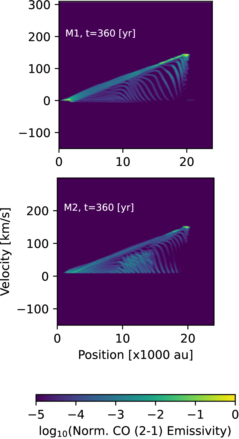
Figure 7: PV diagrams obtained from models M1 and M2 (top and bottom panel, respectively) at $t=360$ yr, assuming a $\phi$ = 30^∘ angle between the outflow axis and the plane of the sky.

It is clear that in models M1 and M2 we obtain CO PV diagrams with a linear ramp of emission with increasing radial velocities as a function of position (see Figure 7, beginning at the outer edge of the dense, central cloud, and ending at the position-velocity position of the high-velocity clump. This ramp of emitting material comes from a mixture of detrained clump material and dense cloud material perturbed by the passage of the clump.

Figure 8 shows a clear difference between the CO emission maps (at $t=360$ yr) of models M3 (with neutral cloud/environmental gas) and M4 (with molecular central cloud and neutral outer environment). The PV diagrams obtained from these two models (see Figure 9) also show a linear velocity vs. position emission ramp (see Figure 10). Finally, model M5 (with partially molecular central cloud and fast cloud and fully molecular outer environment) also produces PV diagrams with an approximately linear velocity vs. position ramp (see Figure 10).

From this exercise, we conclude that the presence of an inner, dense cloud in the environment (through which is travelling the fast clump) results in PV diagrams with an approximately linear ramp of increasing velocities as a function of distance from the outflow source. This feature is quite persistent, as it is present even in the case in which only the material of the fast clump is molecular (model M3).

Our results are clearly dependent on the density structure. Morphologically, filaments are formed in models from M0 to M5, but the kinematic differences point towards the structure present in models from M1 to M4. This is the behaviour shown by the observational PV diagrams, with a linear dependence of the velocity with the position (Zapata et al. 2009, figure 2, and Bally et al. 2017, figure 5).

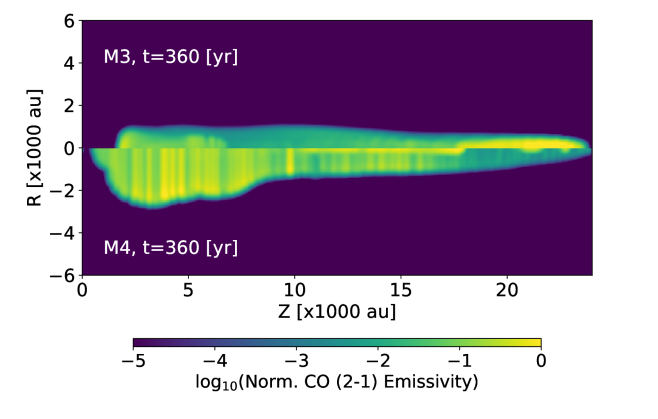
Figure 8: CO emission maps from Models M3 and M4 (top and bottom panels, respectively) at a $t=360$ yr evolutionary time, assuming that the outflow axis lies on the plane of the sky.

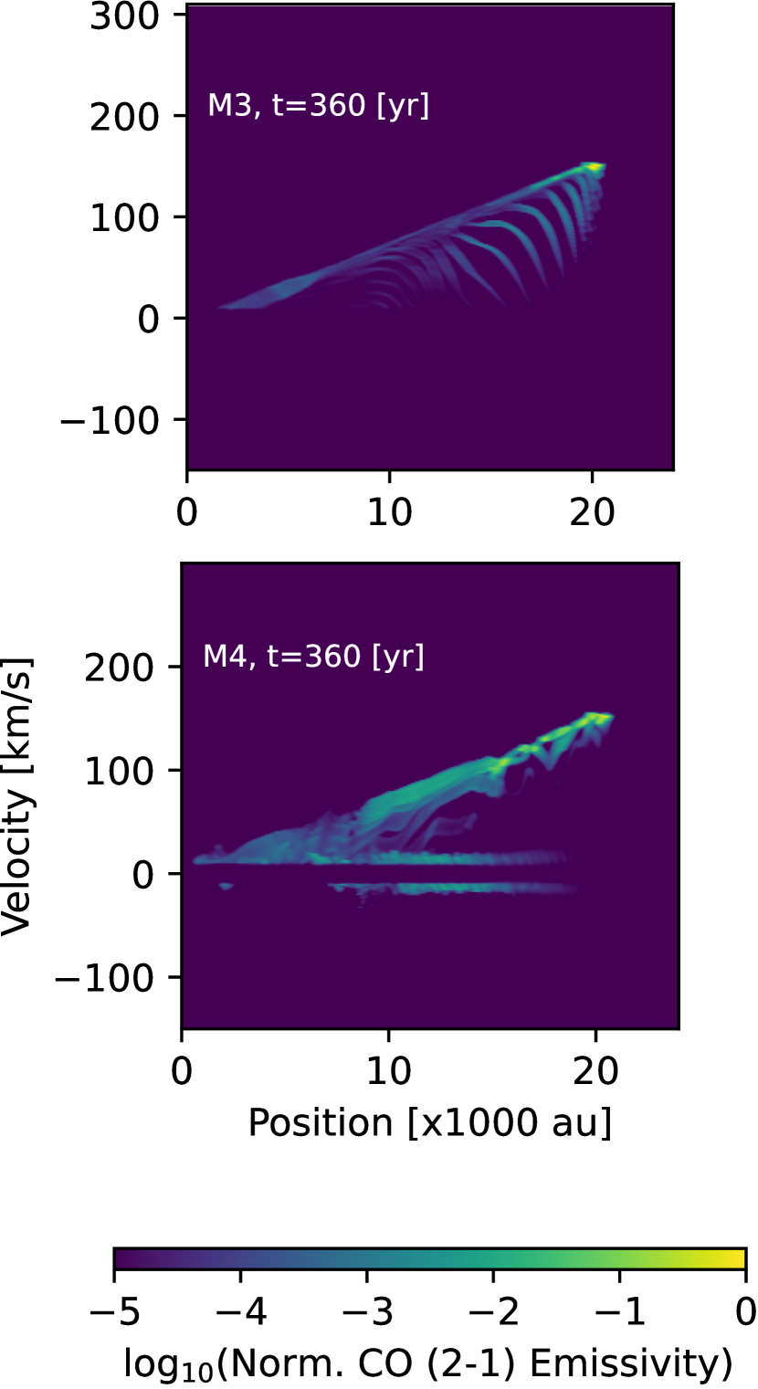
Figure 9: PV diagrams obtained for models M3 and M4 (top and bottom panel, respectively) at $t=360$ yr, assuming a $\phi$ = 30^∘ angle between the outflow axis and the plane of the sky.

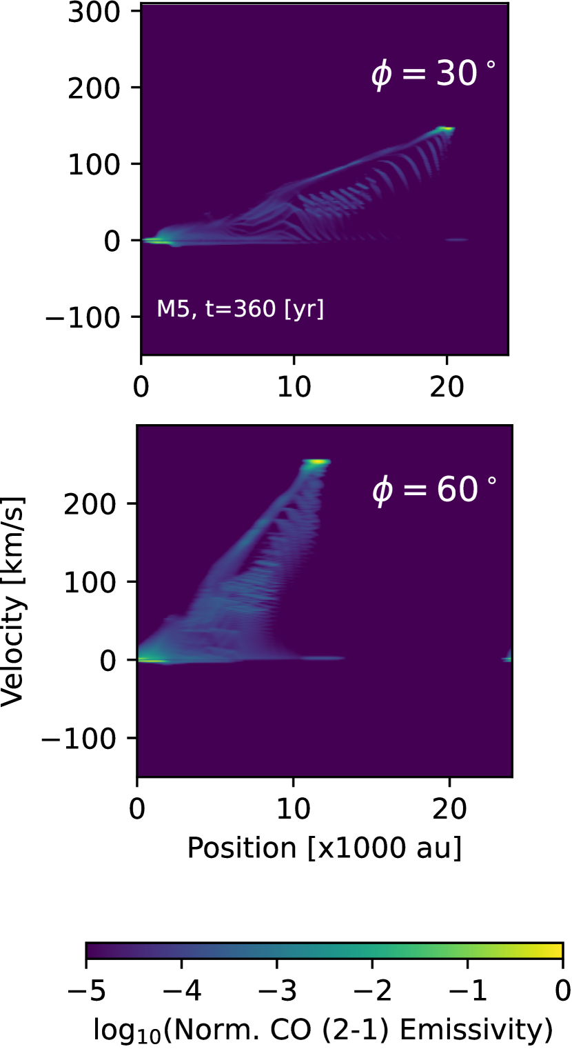
Figure 10: PV diagrams obtained from model M5 for $t=360$ yr, assuming $\phi$ = 30^∘ (top) and 60^∘ angle (bottom) between the outflow axis and the plane of the sky.

4 Summary

Explosive outflows seem to be the result of a poorly understood interaction of protostellar objects in massive star-forming regions. To interpret the observed characteristics of the explosive outflow Orion BN/KL we present a set of simulations of the "CO streamers", assuming an ejection of high-velocity clumps which interact with a structured ambient medium. We carried out reactive flow numerical simulations solving the rate equations of 15 species (H, H⁺, C, C₂, CH, CH₂, CO₂, HCO, H₂O, O, O₂, H₂, CO, OH, and e^- ) considering 47 chemical reactions (as in Castellanos-Ramírez et al., 2018), and including a molecular/atomic/ionic cooling rate.

In this work, we have focused on studying the importance of:

• a) the possible presence of a dense, central cloud within which the high-velocity ejecta starts to evolve,

• b) the effect of the initial molecular fractions in each of the components: ejected clump, central cloud and outer, uniform interstellar medium.

In order to compare our numerical results with the observational features of the Orion fingers presented in Zapata et al. (2009) and Bally et al. (2017), we have obtained predictions of CO ($J=2\to$1) intensity maps and PV diagrams. To this effect, we have calculated the appropriate emission coefficient (from the temperature and non-equilibrium CO abundance in each computational cell) and carried out the appropriate line of sight integration. Clearly, this process could be also done for many other molecular lines, but our present paper is restricted to the CO ($J=2\to$1) line.

Our models of fast clumps travelling in a uniform-density medium (models M00 and M0, see Table 1) produce emission maps with CO streamers with widths of $\sim 1000$ au (see Figure 4). The PV diagrams predicted from these models show the fast velocity clump, and a highly structured wake joining the clump to the outflow source.

Our models with a central “dense cloud” region produce emission maps with CO streamers of varying widths (see Figures 6 and 8), with the narrowest streamers for the case of model M3, in which only the fast clump is molecular (see the top panel of Figure 8 and Table 1). All of these models produce CO PV diagrams with a clear, linear velocity vs. position ramp joining the edge of the central, dense cloud to the PV position of the fast clump. This “Hubble law” expansion is a quite sturdy feature, because it is present in cases in which the central cloud is molecular (models M1, M2 and M4) or not (model M3, in which only the fast clump is molecular, see Table 1). This linear ramp in the PV diagrams is in clear qualitative agreement with the structures observed in the Orion fingers.

It is important to stress that the calculated PV diagrams show an expansion ramp that does not point to the origin of the clump motion, but to the outer edge of the central, dense cloud. This result is also in qualitative agreement with the observations of the CO streamers, in which each of PV ramps of the fingers points to a central volume of a few thousand astronomical unities as reported by Zapata et al. (2009, 2020). This possibly corresponds to a central cloud from which have emerged the clumps that formed the fingers in the Orion BN/KL region.

5 DATA AVAILABILITY

The data underlying this article will be shared on reasonable request to the corresponding author.

References

- (1) Allen, D. A. & Burton, M. G. 1993, Nature, 363, 54. doi:10.1038/363054a0
- Axon & Taylor (1984) Axon, D. J. & Taylor, K. 1984, MNRAS, 207, 241. doi:10.1093/mnras/207.2.241
- Bally et al. (2005) Bally, J., Licht, D., Smith, N. & Walawender, J., 2005, AJ, 129, 355.
- Bally et al. (2011) Bally, J., Cunningham, N. J., Moeckel, N., Burton, M. G., Smith, N., Frank, A. & Nordlund, A., 2011, ApJ, 727, 113.
- Bally et al. (2015) Bally, J., Ginsburg, A., Silvia, D. & Youngblood, A., 2015, A&A, 579,130.
- Bally (2016) Bally, J., 2016, ARA&A, 54, 491.
- Bally et al. (2017) Bally, J., Ginsburg, A., Arce, H., Eisner, J., Youngblood, A., Zapata, L. & Zinnecker, H., 2017, ApJ, 837, 60.
- Castellanos-Ramírez et al. (2018) Castellanos-Ramírez, A., Rodríguez-González, A., Rivera-Ortíz, P. R., Raga, A. C., Navarro-González, R. & Esquivel, A., 2018, RMxAA, 54, 409.
- Chrysostomou et al. (1997) Chrysostomou, A., Burton, M. G., Axon, D. J., et al. 1997, MNRAS, 289, 605. doi:10.1093/mnras/289.3.605
- DeYoung and Axford (1967) De Young, D. S. and Axford, W. I., 1967, Nat, 129-131, 216
- Doi et al. (2002) Doi, T., O’Dell, C. R., & Hartigan, P. 2002, AJ, 124, 445. doi:10.1086/341044
- Esquivel et al. (2009) Esquivel, A., Raga, A. C., Cantó, J., & Rodríguez-González, A. 2009, A&A, 507, 855
- Feng et al. (2015) Feng, S., Beuther, H., Henning, Th., Semenov, D., Palau, A. & Mills, E. A. C., 2015, A&A, 581, 71.
- (14) Goddi, C., Humphreys, E. M. L., Greenhill, L. J., Chandler, C. J. & Matthews, L. D., 2011, ApJ, 728, 15.
- Henney et al. (2009) Henney, W. J., Arthur, S. J., de Colle, F. & Mellema, G., 2009, MNRAS, 398, 157.
- Hosokawa & Omukai (2009) Hosokawa, T. & Omukai, K., 2009, ApJ, 691, 823.
- Hosokawa et al. (2010) Hosokawa, T., Yorke, H. W. & Omukai, K., 2010, ApJ, 721, 478.
- Menten et al. (2007) Menten, K. M., Reid, M. J., Forbrich, J. & Brunthaler, A., 2007, A&A, 474, 515
- Kosińsky & Hanasz (2007) Kosiński, R. & Hanasz, M., 2007, MNRAS, 376, 861.
- Kwan & Scoville (1976) Kwan, J. & Scoville, N. 1976, ApJ, 210, L39. doi:10.1086/182298
- O’Dell (1997) O’dell, C. R. 1997, The Orion Nebula Proplyds: Properties and Survival. American Astronomical Society Meeting Abstracts, 191.
- Oh et al. (2016) Oh, H., Pyo, T.-S., Kaplan, K., et al. 2016, ApJ, 833, 275. doi:10.3847/1538-4357/833/2/275
- Raga & Reipurth (2004) Raga, A. C. & Reipurth, B., 2004, RMxAA, 40, 15.
- Raga et al. (2021) Raga, A. C., Rivera-Ortiz, P. R., Cantó, J., et al. 2021, MNRAS, 508, L74. doi:10.1093/mnrasl/slab072
- Raga et al. (2022) Raga, A. C., Cantó, J., Castellanos-Ramírez, A. et al. 2022, Galax., 10, 19R
- Rybicki & Lightman (1986) Rybicki, G. B. & Lightman, A. P. 1986, Radiative Processes in Astrophysics, by George B. Rybicki, Alan P. Lightman, pp. 400. ISBN 0-471-82759-2. Wiley-VCH , June 1986., 400
- Rivera-Ortiz et al. (2022) Rivera-Ortiz, P.R., Schutzer, A., Lefloch, B. & Gusdorf, A., 2022, A&A, in prep
- Rivera-Ortiz et al. (2019) Rivera-Ortiz, P., Rodríguez-González, A., Hernández-Martínez, L. & Cantó, J., 2019, ApJ, 874, 38.
- Rivera-Ortiz et al. (2019) Rivera-Ortiz, P. R., Rodríguez-González, A., Hernández-Martínez, L., et al. 2019, ApJ, 885, 104
- Rivera-Ortiz et al. (2021) Rivera-Ortiz, P. R., Rodríguez-González, A., Cantó, J., et al. 2021, ApJ, 916, 56. doi:10.3847/1538-4357/ac05bb
- Salas et al. (1999) Salas, L., Rosado, M., Cruz-González, I., et al. 1999, ApJ, 511, 822. doi:10.1086/306695
- Tan (2004) Tan, J. C. 2004, ApJ, 607, L47. doi:10.1086/421721
- Zapata et al. (2009) Zapata, L. A., Schmid-Burgk, J., Ho, P. T. P., Rodríguez, L. F. & Menten, K. M., 2009, ApJ, 704, 45.
- Zapata et al. (2017) Zapata, L. A., Schmid-Burgk, J., Rodríguez, L. F., et al. 2017, ApJ, 836, 133. doi:10.3847/1538-4357/aa5b94
- Zapata et al. (2020) Zapata, L. A., Ho, P. T. P., Fernández-López, M., et al. 2020, ApJ, 902, L47. doi:10.3847/2041-8213/abbd3f
- Zapata et al. (2013) Zapata, L. A., Schmid-Burgk, J., Pérez-Goytia, N., et al. 2013, ApJ, 765, L29. doi:10.1088/2041-8205/765/2/L29
- Zapata et al. (2011) Zapata, L. A., Loinard, L., Schmid-Burgk, J., et al. 2011, ApJ, 726, L12. doi:10.1088/2041-8205/726/1/L12