ToL:
A Tensor of List-Based
Unified Computation Model

   

Edited By

Hongxiao Li
Wanling Gao
Lei Wang
Jianfeng Zhan

BenchCouncil: International Open Benchmark Council
Chinese Academy of Sciences
Beijing, China
https://www.benchcouncil.org

Technical Report No. BenchCouncil-ToL-2022

Dec 20, 2022

Abstract

Previous computation models either have equivalent abilities in representing all computations but fail to provide primitive operators for programming complex algorithms or lack generalized expression ability to represent newly-added computations. This article presents a unified computation model with generalized expression ability and a concise set of primitive operators for programming high-level algorithms. We propose a unified data abstraction – Tensor of List, and offer a unified computation model based on Tensor of List, which we call the ToL model (in short, ToL). ToL introduces five atomic computations that can represent any elementary computation by finite composition, ensured with strict formal proof. Based on ToL, we design a pure-functional language – ToLang. ToLang provides a concise set of primitive operators that can be used to program complex big data and AI algorithms. Our evaluations show ToL has generalized expression ability and a built-in performance indicator, born with a strictly defined computation metric – elementary operation count (EOPs), consistent with FLOPs within a small error range.

1 Introduction

Good data and computation abstractions catch the intrinsic properties of computing and hence play an essential role. The earliest computation models, such as Turing machine [1], Game of Life [2], Langton’s ant [3], and lambda calculus [4], are typical example. These models have equivalent abilities in representing all computations. Unfortunately, these models only assure feasibility in computation representation and fail to provide primitive operators to program complex algorithms.

Keeping performance concerns in mind, the researchers present several computation models and corresponding languages providing operators for specific domains, such as relation algebra [5], SQL [6] for database, and MATLANG [7] for scientific computation. Besides them, there are also implicit models and operators provided by the libraries or computation engines like TensorFlow [8] and PyTorch [9] for deep learning. Their intuition is to define atomic computations, offer language with operators that are compositions of one or more atomic computations, and implement every operator to ensure the best performance on major computation tasks. However, these models or corresponding operators are confronted with two major problems. First, they are designed for a relatively small domain. For example, relation algebra is only suitable for structured data. As a result, they remain low compatibility and high portability cost issues when extending those models to support emerging computing. Second, they have poor generalized expression ability. The generalized expression ability depicts the ability to represent newly-added computations on the existing computation model. If users want to implement new computations in a particular model with poor generalized expression ability, they must implement new operators case by case. As a result, there are more and more newly-defined complicated operators with different semantics.

To attack the above challenges, this article proposes a unified computation model with the generalized expression ability and a concise set of primitive operators. First, we propose a unified data abstraction – Tensor of List. Tensor of List is a data abstraction with generalized expression ability, and classical data abstractions like vector, matrix, tensor, and list, can be seen as its particular instances. Based on Tensor of List, we present a unified computation model. The proposed computation model introduces five atomic computations. The five atomic computations can represent any elementary computation on the ToL data abstraction by finite composition, ensured with strict formal proof. We call the Tensor of List data abstraction and the corresponding computation abstraction the ToL model (In short, ToL). In the rest of this article, ToL refers to the ToL data abstraction or the ToL model in different contexts. Based on ToL, we design a pure-functional language – ToLang, which provides a concise set of primitive operators that can be used to program complex big data and AI algorithms.

We focus on four aspects to evaluate how our computation model solves the problems. Table 1 is the overall comparison of different models/languages. As for the applicable domain, ToL suits all domains and provides three levels of generalized expression ability: data abstraction, a limited composition of the five atomic computations that can represent any ToL elementary computation, and a concise set of primitive operators. As for conciseness, we show a smaller set of primitive operators in ToLang can present a large set of ONNX [10] operators in the AI domain. Finally, as for performance concerns, we show ToL has a built-in performance indicator, born with a strictly defined computation metric – elementary operation count (EOPs), consistent with FLOPs [11] within a small error range.

Model	Language	Data abstractions	Atomic computations (quantity)	Domain	Generalized expression ability	Operator quantity
Turing machine	-	Finite array	Read, write, lshift, rshift (4)	All	high	-
Lambda calculus	-	Function	Lambda (1)	All	high	-
Relation algebra	SQL	Structured data	Select, project, Cartesian, union, intersection, rename (6)	Structured	high	10+
Matlang	Matlab	Matrix	Variable, transpose, one-vector, diagonalize, multiply, add, scalar, point-wise (8)	Linear	middle	100+
Arithmetic circuits	-	Matrix	Add, sub, mul,… (10+)	Linear	low	-
-	Haskell	All types	Add, sub, mul, max, … (100+)	All	low	100+
-	TensorFlow, PyTorch	Tensor	Conv, ReLU, MatMul, … (100+)	Tensor	low	100+
ToL	ToLang	Tensor of List	Lambda, norm, member, join, embed (5)	All	high	13

Table 1: The comparisons of different models/languages. ToL has a generalized expression ability. It has only five atomic computations and 10+ primitive operators, suiting all application domains.

The organization of this article is as follows. Section 2 is the related work. We make all the necessary definitions for ToL data and computation abstractions in Sections 3.1-3.3. We present strict proof for ToL’s completeness and atomicity properties in Section 3.4. We present ToLang in Section 4. We evaluate ToLang’s expression ability in Section 5. We demonstrate ToL’s built-in performance indicator in Section 6. Section 7 is the conclusion.

2 Related work

The earliest computation models in the computer science domain are Turing machine [1], Boolean circuits [12], and lambda calculus [13]. They have equivalent abilities in representing all computations but fail to provide primitive operators for programming complex algorithms. Late in different sub-domains, several data and computation models are proposed without generalized expression abilities to represent newly-added computations. Typical data abstractions include matrix, widely used in linear algebra, tensor, used in deep learning, set and tuple, in database [14]. Typical computation models have relation algebra [5] and tuple relation calculus [15] in the database, tensor computation in the AI, and matrix computation in the scientific computation domains, respectively.

Our proposed ToL model has a generalized expression ability and a concise set of primitive operators. Suiting all application domains, it has only five atomic computations and 10+ primitive operators: a limited composition of the five atomic computations can represent any ToL elementary computation, and a concise set of primitive operators can program complex big data and AI algorithms.

Besides computation models, the researchers characterized primary computation characteristics in big data, AI, and other domains by workload characterizations. First, the Berkeley multi-disciplinary teams [16] classify computation of different algorithms into 13 basic modes, named data dwarfs. After that, Gao et al. [17] investigated five application domains of big data and AI and decomposed various types of computation into eight classes of computation units, named data motifs.

As for high-level language, there are some description languages based on data abstractions and computation models, including SQL language [18] based on relation algebra, MATLANG [19] based on linear matrix computation, and Haskell [20] as a pure-functional language for general purpose.

3 ToL

This section presents ToL, a computation model that can express all elementary computations in different domains. Our methodology is as follows. First, we define the ToL data abstraction. Second, we present the ToL atomic computations: a minimum set of atomic computations defined on ToL. Third, we prove all elementary computations can be expressed using a finite composition of ToL atomic computations.

3.1 ToL Data abstraction

Definition 1.1 (Type space): A type space is defined as a set, noted as $V$. An element in a type space is defined as a numeric, noted as $v\in V$. The set of all type spaces is defined as the type space set, noted as $\mathbb{V}=\{V|V$ is a type space$\}$.

Definition 1.2 (List): A list space is defined as the Cartesian product of a finite quantity of type space, noted as $L=V_{1}\times V_{2}\times\cdots\times V_{k}$, for $V_{j}\in\mathbb{V},1\leq j\leq k,k\in\mathbb{N^{*}}$. We note $[V_{1},V_{2},\cdots,V_{k}]$ as the type list and $k$ as the capacity of list. An element in a list space is defined as a list, noted as $l\in L$. The set of all list spaces is defined as the list space set, noted as $\mathbb{L}=\{L|L$ is a list space$\}$. A list is noted as $(l_{1},\cdots,l_{k})$.

Definition 1.3 (Tensor of List, ToL): A ToL space is defined as a multidimensional extension of list spaces, noted as $T=L^{d_{1}\times d_{2}\times\cdots\times d_{n}}$, for $d_{i}\in\mathbb{N^{*}},1\leq i\leq n,n\in\mathbb{N^{*}}$. We note $[d_{1},d_{2},\cdots,d_{n}]$ as the shape and $n$ the dimension of ToL, respectively. An element in a ToL space is defined as a ToL, noted as $t\in T$. The set of all ToL spaces is defined as the ToL space set, noted as $\mathbb{T}=\{T|T$ is a ToL space$\}$. Numeric, vector, matrix, tensor, and list are ToL instances. The capacity of a tensor is 1. A ToL is noted as $[\cdots[t_{1,\cdots,1,1},...,t_{1,\cdots,1,d_{n}}],...,t_{1,\cdots,d_{n-1},1},...,t_{1,\cdots,d_{n-1},d_{n}}],\cdots,t_{d_{1},d_{2},\cdots,d_{n}}]$.

Example 1: Real set $\mathbb{R}\in\mathbb{V}$ is a type space.

$L=\mathbb{Z}\times\mathbb{R}\times\mathbb{N^{*}}$ is a list space with 3 capacity. List $l=(0,3.0,1)\in L$.

Numeric $3.14$ is a trivial list with capacity 1.

$T=L^{2\times 2}$ is a ToL space with two dimensions. ToL $t=[[(1,1.0,1),(2,2.0,2)],[(3,3.0,3),(4,4.0,4)]]\in T$.

3.2 ToL elementary computations

Definition 2.1 (Basic elementary functions): According to Liouville [21], a basic elementary function is “a function of several variables that is defined as taking sums, products, roots, polynomial, rational, trigonometric, hyperbolic, exponential functions, and their inverse functions”. All the basic elementary functions in ToL model are listed in Table 2.

Definition 2.2 (Elementary functions): According to Liouville [21], an elementary function is “the sum, product, or composition of a finite quantity of basic elementary functions”.

function	parameters	space
add(+), sub(-)	$<$var$>$, $<$var$>$	$\mathbb{C}$
mul($\times$), div($\div$)	$<$var$>$, $<$var$>$	$\mathbb{C}$
mod($\%$)	$<$var$>$, $<$var$>$	$\mathbb{Z}$
pow(^), log	$<$var$>$, $<$var$>$	$\mathbb{R}$
and, or, xor	$<$var$>$, $<$var$>$	$\mathbb{B}$
not	$<$var$>$	$\mathbb{B}$
lt(>), gt(<), eq(=)	$<$var$>$, $<$var$>$	$\mathbb{R}$
le($\leq$), ge($\geq$), ineq($\neq$)	$<$var$>$, $<$var$>$	$\mathbb{R}$
max, min	$<$var$>$, $<$var$>$	$\mathbb{R}$
sgn	$<$var$>$	$\mathbb{R}$
sin, cos, tan, asin, acos, atan	$<$var$>$	$\mathbb{R}$
sinh, cosh, tanh, asinh, acosh, atanh	$<$var$>$	$\mathbb{R}$
rand	$<$var$>$	$\mathbb{R}$

Table 2: The list of basic elementary functions.

Definition 2.3 (ToL elementary computations): A ToL elementary computation is a function $F\in(\mathbb{T},\mathbb{T},\cdots,\mathbb{T})\mapsto\mathbb{T}$, noted as $F(t_{1},t_{2},\cdots,t_{p};c_{1},c_{2},\cdots,c_{q})=f_{0}$, where $t_{1},t_{2},\cdots,t_{p},f_{0}\in\mathbb{T},c_{1},c_{2},\cdots,$
$c_{q}$ are constants, $p,q\in\mathbb{Z+}$, and numeric values in result $f_{0}$ can be computed with elementary functions with only the following inputs: part of values from certain $t_{i}$; capacity, shape, dimension of certain $t_{i}$; certain constant value $c_{j}$. In other words, ToL elementary computations are elementary functions computed on ToLs.

Example 2: For real matrices $A$ and $B$ of $[n,n]$ shape, $F(A,B)=A+B$ is an elementary computation on ToL. In this example, $F\in(T,T)\mapsto T,T=\mathbb{R}^{n\times n}$. The basic elementary function involved is add (+).

3.3 ToL atomic computations

In this subsection, we state that five ToL atomic computations are the smallest set enough for expressing all ToL elementary computations.

We suppose ToL $t=t_{1}=L^{d_{1}\times d_{2}\times\cdots\times d_{n}}$, $t_{2}=L^{d_{1}\times d_{2}\times\cdots\times d_{n-1}\times D_{n}}$, where $L=V_{1}\times V_{2}\times\cdots\times V_{k}$ in this subsection.

Definition 3.1 (lambda): A lambda is noted as $\Lambda(f;e_{1},e_{2},\cdots,e_{p};c_{1},c_{2},\cdots,c_{q})$, where $e_{1},e_{2},\cdots,e_{p}$ are numeric, $c_{1},c_{2},\cdots,c_{q}$ are constants, $f$ is an elementary function, $p,q\in\mathbb{N^{*}}$. $\Lambda(f;e_{1},e_{2},\cdots,e_{p};c_{1},c_{2},$
$\cdots,c_{q})$ computes $f(e_{1},e_{2},\cdots,e_{p};c_{1},c_{2},\cdots,c_{q})$ and returns the result. The function $f$ is a basic elementary function or the composition of several basic elementary functions in Table 2.

Definition 3.2 (norm): A norm is noted as $\|t\|$ or $\|t\|^{\prime}$. $\|t\|=[d_{1},d_{2},\cdots,d_{n}]$ and $\|t\|^{\prime}=k$. Additionally, $\|(\|t\|)\|=n$.

Definition 3.3 (member): A member is noted as $\Pi(t;a_{1},a_{2},\cdots,a_{n})$ or $\Pi^{\prime}(t;j)$, where $a_{1},a_{2},\cdots,a_{n}\in\mathbb{N^{*}},1\leq a_{i}\leq d_{i},1\leq i\leq n,1\leq j\leq k$, and $n$ is the dimension of $t$. $\Pi$ returns the list member of coordinates given by $a_{1},a_{2},\cdots,a_{n}$ and $\Pi^{\prime}$ returns the corresponding ToL with the same shape as $t$ and type list=$V_{j}$. $\Pi(t;a_{1},a_{2},\cdots,a_{n})$ is also noted as $t[a_{1},a_{2},\cdots,a_{n}]$.

Definition 3.4 (join): A join is noted as $T_{1}\bowtie T_{2}$ or $T_{1}\overline{\bowtie}T_{2}$. For $T_{1}\bowtie T_{2}$, ToLs $t_{1}$ and $t_{2}$ must have the same type list, shape, and dimensions except for the last dimension. $t_{1}\bowtie t_{2}$ has the same type list, dimension, and shape but the last dimension=$d_{n}+D_{n}$. We have $(t_{1}\bowtie t_{2})[a_{1},a_{2},\cdots,a_{n}]=\begin{cases}t_{1}[a_{1},a_{2},\cdots,a_{n}],a_{n}\leq d_{n}\\ t_{2}[a_{1},a_{2},\cdots,a_{n-1},a_{n}-d_{n}+1],a_{n}>d_{n}\end{cases}$ for $1\leq a_{i}\leq d_{i},1\leq i\leq n-1$ and $1\leq a_{n}\leq d_{n}+D_{n}$. For $\overline{\bowtie}$, ToL $t_{1}$ and $t_{2}$ must have the same dimension and shape. Similar to $\bowtie$, $T_{1}\overline{\bowtie}T_{2}$ joins list members of the same coordinates of $t_{1}$ and $t_{2}$.

Definition 3.5 (embed) An embed is noted as $\Xi(t)$. $\Xi(t)$ returns a ToL with one more dimension than $t$, the last dimension $d_{n+1}=1$. The relation between $\Xi(t)$ and $t$ is: $\Xi(t)[a_{1},a_{2},\cdots,a_{n},1]=t[a_{1},a_{2},\cdots,a_{n}]$.

Example 3: Lambda: $\Lambda(+,e_{1},c_{1})$, $\Lambda(\times,e_{1},e_{2})$, $\Lambda(\arcsin,e_{1})$, in which $e_{1},e_{2}$ are variable and $c_{1}$ is constant.
Norm: $\|[(1,1.),(2,2.),(3,3.)]\|=3$. $\|[(1,1.),(2,2.),(3,3.)]\|^{\prime}=2$.
Member: $t=[[1,2],[3,4]]$, $t[2,2]=4$.
Join: $[1,2,3]\bowtie[1,2]=[1,2,3,1,2]$. $(3,0.14)\overline{\bowtie}3.2=(3,0.14,3.2)$.
Embed: $\Xi([1,2,3])=[[1],[2],[3]]$.

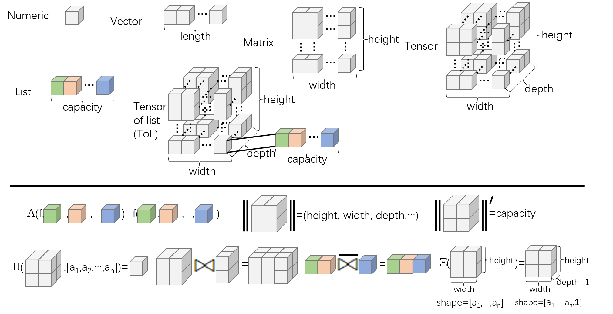
Figure 1: The visualizations of ToL, ToL instantiations, and ToL atomic computations.

Figure 1 visually shows ToL, ToL instantiations, and ToL atomic computations. ToL instantiations include numeric, vector, matrix, tensor, and list.

3.4 Proof

This section proves that the ToL atomic computations have two properties: atomicity and completeness.

Theorem One: the atomic property: Each ToL atomic computation cannot be represented by the other atomic computations or their composition.

Theorem Two: the complete property: Any ToL elementary computation can be represented by a finite composition of ToL atomic computations.

The above theorems ensure that five ToL atomic computations are enough for expressing all ToL elementary computations.

3.4.1 Proof for Theorem One

We prove that each of the five ToL atomic computations (lambda, norm, member, join, embed) cannot be represented by the other ToL atomic computations or their composition. We construct an example of each ToL atomic computation and show that the rest of the ToL computations cannot represent it.

Lambda: Consider $F(a,b)=a+b$. $\Lambda(+,a,b)$ can represent $F$. However, either norm, member, join, or embed cannot perform addition.

Norm: Consider that $F$ computes the size of vector $v$, $v\in\{[0],[0,0],[0,0,0],\cdots\}$. $F(v)=\|v\|$. A lambda can compute vector values (zeros), but it cannot return the size of vectors. Member, join, or embed can only return vectors of 0 values and cannot return the size of vectors, either.

Member: Consider that $F$ computes the sum of vector $v$ member values, and $v=[1,2,3,4]$. $F(v)=\Lambda(+,v[1],\Lambda(+,v[2],\Lambda(+,v[3],v[4])$. However, lambda only accepts numeric and function inputs, but $v$ is a vector. Join and embed can only return a ToL, which is not numeric.

Join: Consider $F(t_{1},t_{2})=t_{1}\bowtie t_{2}$, where $t_{1}$ and $t_{2}$ are vectors. $\|t_{1}\bowtie t_{2}\|[1]=\|t_{1}\|[1]+\|t_{2}\|[1]$. The first dimensions of the shapes are added up. However, lambda, norm, and member return numeric values. Embed cannot change the first dimension of a vector.

Embed: Consider $F(t)=\Xi(t)$, where $t$ is a $n$-dimensional tensor. The dimension of $F(t)$ is bigger than that of $t$. However, lambda, norm, and member return numeric values. Join only changes the last dimension and cannot increase the dimension.

3.4.2 Proof for Theorem Two

Consider a ToL elementary computation noted as $F(t_{1},t_{2},\cdots,t_{p};c_{1},c_{2},\cdots,c_{q})=f_{0}$. We discuss by categorization:

Case 1: $f_{0}$ is a numeric value.

Sub-case 1.1: $t_{1},t_{2},\cdots,t_{p}$ are numeric values, and Function $F$’s inputs are them and constants. In this sub-case, we represent an elementary function $F$ with a finite composition of basic elementary functions. Note $F(t_{1},t_{2},\cdots,t_{p};c_{1},c_{2},\cdots,c_{q})=f_{1}(f_{2}(\cdots f_{r}(\cdots,y_{r}),\cdots,y_{2}),\cdots,y_{1})$, where $y_{1},y_{2},\cdots,y_{r},\cdots$ are rearranged $t_{i}$’s and $c_{j}$’s, $r\in\mathbb{N^{*}}$, and $f_{1},f_{2},\cdots,f_{r}$ are basic elementary functions. Then computation $f_{0}=F(t_{1},t_{2},\cdots,t_{p};c_{1},c_{2},\cdots,c_{q})$ can be represented as $f_{0}=\Lambda(f_{1},\Lambda(f_{2},\cdots\Lambda(f_{r},y_{r},\cdots),y_{2},\cdots),y_{1},\cdots)$.

Sub-case 1.2: Some of $t_{1},t_{2},\cdots,t_{p}$ are not pure numeric but normal ToLs, and Function $F$’s inputs are numeric elements from certain ToLs and constants. Note the numeric inputs of Function $F$ as $x_{j}$’s, $s\in\mathbb{N^{*}}$. Then it can be represented as $F(x_{1},x_{2},\cdots,x_{s};c_{1},c_{2},\cdots,c_{q})$. For each $x_{j}$, if it derives from a certain ToL $t_{i}$, use $x_{j}=\Pi(t_{i};a_{j_{1}},a_{j_{2}},\cdots,a_{j_{n}})$ for ToL elements and $x_{j}=\Pi^{\prime}(t_{i};j_{m})$ for list elements, where $a_{j_{1}},a_{j_{2}},\cdots,a_{j_{n}},m,n\in\mathbb{N^{*}}$. Then this sub-case turns to sub-case 1.1.

Sub-case 1.3: Function $F$’ inputs include not only numeric variables, ToL’s numeric elements, and constants but also the capacity, shape, and dimension of certain ToLs. Suppose $F$’s parameters include capacity, shape, and dimension of a certain $t_{i}$. We use the following representation:
capacity($t_{i}$)=$\|t_{i}\|^{\prime}$
shape($t_{i}$)=$\|t_{i}\|$
dimension($t_{i}$)=$\|\|t_{i}\|\|$
Then this sub-case turns to sub-case 1.1 or 1.2.

Case 2: $f_{0}$ is not a numeric value but a normal ToL.

Note $f_{0}=T=L^{d_{1}\times d_{2}\times\cdots\times d_{n}}$, $d_{i}\in\mathbb{N^{*}},1\leq i\leq n,n\in\mathbb{N^{*}}$ and $L=V_{1}\times V_{2}\times\cdots\times V_{k},V_{j}\in\mathbb{V},1\leq j\leq k,k\in\mathbb{N^{*}}$. We construct $f_{0}$ by the following steps.

Step 1: First we consider a numeric member of $f_{0}$ at certain coordinates, such as $\Pi^{\prime}(f_{0}[a_{1},a_{2},\cdots,a_{n}],j)$. According to case 1, it can be represented with lambda, norm, and member computation; we note such representation as $\Omega(a_{1},a_{2},\cdots,a_{n};j)$ in short.

Step 2: For all $j$ that $1\leq j\leq k$, construct list member $f_{0}[a_{1},a_{2},\cdots,a_{n}]=\Omega(a_{1},a_{2},\cdots,a_{n};1)\overline{\bowtie}\Omega(a_{1},a_{2},$
$\cdots,a_{n};2)\overline{\bowtie}\cdots\overline{\bowtie}\Omega(a_{1},a_{2},\cdots,a_{n};k)$. So far every $f_{0}[a_{1},a_{2},\cdots,a_{n}]$ is represented.

Step 3: For the last dimension $d_{n}$, construct $f_{0}[a_{1},a_{2},\cdots,a_{n-1}]=f_{0}[a_{1},a_{2},\cdots,1]\bowtie f_{0}[a_{1},a_{2},\cdots,2]\bowtie\cdots\bowtie f_{0}[a_{1},a_{2},\cdots,d_{n}]$. Therefore, $\|f_{0}[a_{1},a_{2},\cdots,a_{n-1}]\|=d_{n}$. If $n=1$, the representation is complete.

Step 4: If $n>1$, construct $\Xi(f_{0}[a_{1},a_{2},\cdots,a_{n-1}])$, noted as $f_{0}^{\prime}[a_{1},a_{2},\cdots,a_{n^{\prime}}]$ for short, where $n^{\prime}=n-1$, and $\|f_{0}^{\prime}[a_{1},a_{2},\cdots,a_{n^{\prime}}]\|=[d_{n},1]$. Continue to construct $f_{0}^{\prime}[a_{1},a_{2},\cdots,a_{{n^{\prime}}-1}]=f_{0}^{\prime}[a_{1},a_{2},\cdots,1]\bowtie f_{0}^{\prime}[a_{1},a_{2},\cdots,2]\bowtie\cdots\bowtie f_{0}^{\prime}[a_{1},a_{2},\cdots,d_{n^{\prime}}]$. Repeat steps 3 and 4 until all the dimensions of $f_{0}$ are represented.

Example 4: Computation $F(a,b)=f_{0}$ computes matrix multiplication of matrices $a$ and $b$ sized $[2,2]$. It can be represented with atomic computations as follows:
$f_{1,1}=\Lambda(+,\Lambda(\times,a[1,1],b[1,1]),\Lambda(\times,a[1,2],b[2,1]))$
$f_{1,2}=\Lambda(+,\Lambda(\times,a[1,1],b[1,2]),\Lambda(\times,a[1,2],b[2,2]))$
$f_{2,1}=\Lambda(+,\Lambda(\times,a[2,1],b[1,1]),\Lambda(\times,a[2,2],b[2,1]))$
$f_{2,2}=\Lambda(+,\Lambda(\times,a[2,1],b[1,2]),\Lambda(\times,a[2,2],b[2,2]))$
$f_{0}=\Xi(f_{1,1}\bowtie f_{1,2})\bowtie\Xi(f_{2,1}\bowtie f_{2,2})$

4 ToLang

This section proposes a ToL-based language – ToLang. ToLang is a pure-functional language and can proceed with any ToL elementary computation. The statements and primitive operators are based on the compositions of five ToL atomic computations.

4.1 Data declaration

ToLang supports a type space declaration in the following formats:
space <var>: <space>
space <var>: <space> [<lower_bound>, <upper_bound>]
In the two formats, space is a reserved word for declaration, <var> is a variable name, <space> is a defined type space name, <lower
_bound> and <upper_bound> are bounds of the data range. The predefined type spaces are the following:
B N N* Z Z* Z+ Z- Q Q* Q+ Q- R R* R+ R- I C
which stands for:
$\mathbb{B}$, $\mathbb{N}$, $\mathbb{N^{*}}$, $\mathbb{Z}$, $\mathbb{Z^{*}}$, $\mathbb{Z^{+}}$, $\mathbb{Z^{-}}$, $\mathbb{Q}$, $\mathbb{Q^{*}}$, $\mathbb{Q^{+}}$, $\mathbb{Q^{-}}$, $\mathbb{R}$, $\mathbb{R^{*}}$, $\mathbb{R^{+}}$, $\mathbb{R^{-}}$, $\mathbb{I}$, $\mathbb{C}$.

ToLang supports a list declaration in the following formats:
list <var>: <list>
list <var>: <space>
list <var>: [<space>, <space>, $\cdots$], <space>
In the three formats, list is a reserved word for declaration, and <list> is a defined list name. In the third format, the quantity of <space>’s can be any finite positive integer.

ToLang supports a Tensor of List declaration. ToL is the most critical data structure, whose instantiations include numeric, vector, matrix, tensor, and list. In ToLang, any computation is defined and computed on ToLs. They are in the following formats:
tol <var>: <space> // for numeric
tol <var>: <space> [<length>] // for vector
tol <var>: <space> [<height>, <width>] // for matrix
tol <var>: <space> [<length>, <length>, $\cdots$, <length>] // for tensor
tol <var>: <list> // for list
tol <var>: <list> [<length>, <length>, $\cdots$, <length>] // for any type of ToL
In the above formats, <length>, <height>, and <width> must be a positive integer.

4.2 ToL primitive operators

ToLang includes several predefined ToL primitive operators that are the compositions of one or more ToL atomic computations 3.3. They are defined on ToLs and require only (one or several) ToLs and functions as their inputs. The mappings between ToL primitive operators and ToL atomic computations are shown in Table 3. We present each ToL operator as follows. In the rest of this article, when we refer to a ToL atomic computation, we only mention its name, e.g., lambda.

ToL primitive operator	ToL atomic computations	Mapping
function	lambda	f(v_1,v_2,$\cdots$,c_1,c_2,$\cdots$)=$\Lambda$(f;v_1,v_2,$\cdots$,c_1,c_2,$\cdots$)
shape	norm	shape((t_i))=$\|$t_i$\|$
dimension	norm	dimension(t_i)=$\|\|$t_i$\|\|$
capacity	norm	capacity(t_i)=$\|$t_i$\|^{\prime}$
volume	norm	vol($t$)=$\|t\|[1]\times\|t\|[2]\times\cdots\times\|t\|[$dim($t$)$]\times\|t\|^{\prime}$
space	member	space($t$)$\mapsto\mathbb{V}$
convert	member, join, embed	convert($t$,$\mathbb{V^{\prime}}$)$\mapsto t$ in $\mathbb{V^{\prime}}$
part	member, join, embed	part($t$,[$a_{1},a_{2},\cdots,a_{n}$], $b_{1},b_{2},\cdots,b_{n}$])=$\Xi(\cdots\Xi(\Pi(t;a_{1},a_{2},\cdots,a_{n})$ $\bowtie\Pi(t;a_{1}+1,a_{2},\cdots,a_{n})\bowtie\Pi(t;a_{1}+2,a_{2},\cdots,a_{n})\bowtie\cdots\Pi(t;b_{1},a_{2},\cdots,$ $a_{n})\bowtie\Pi(t;b_{1},a_{2}+1,\cdots,a_{n})\bowtie\cdots\Pi(t;b_{1},b_{2},\cdots,b_{n})\cdots)$
swap	member, join, embed	swap($t$,dim,[$x_{1},x_{2},\cdots,x_{k}$])=$\Xi(\cdots\Xi(\Pi(t;1,1,\cdots,x_{1},\cdots,1)\bowtie\Pi(t;1,1,$ $\cdots,x_{2},\cdots,1)\bowtie\cdots\Pi(t;1,1,\cdots,x_{k},\cdots,1)\bowtie\cdots\Pi(t;a_{1},a_{2},\cdots,x_{1},\cdots,$ $a_{n})\bowtie\Pi(t;a_{1},a_{2},\cdots,x_{2},\cdots,a_{n})\bowtie\cdots\Pi(t;a_{1},a_{2},\cdots,x_{k},\cdots,a_{n})\cdots)$
reshape	member, join, embed	reshape($t$,shape)=$\Xi(\cdots\Xi(\Pi(t;1,1,\cdots,1)\bowtie\Pi(t;1,1,\cdots,2)\bowtie\cdots$ $\Pi(t;1,1,\cdots,a_{1})\bowtie\cdots\Pi(t;a_{1},a_{2},\cdots,a_{n})\cdots)$
tile	member, join, embed	tile($t$)=$\Xi(\cdots\Xi(\Pi^{\prime}(\Pi(t;1,1,\cdots,1),1)\bowtie\Pi^{\prime}(\Pi(t;1,1,\cdots,1),2)\bowtie\cdots$ $\Pi^{\prime}(\Pi(t;1,1,\cdots,1),k)\bowtie\cdots\Pi^{\prime}(\Pi(t;a_{1},a_{2},\cdots,a_{n}),k)\cdots)$
map	lambda, member, join, embed	map($t$,$f$,iter)=$\Xi(\cdots\Xi(\Lambda(f,t[1,1,\cdots,1]))\bowtie\Xi(\Lambda(f,t[2,1,\cdots,1]))$ $\bowtie\cdots\bowtie\Xi(\Lambda(f,t[d_{1},1,\cdots,1])))\bowtie\cdots\bowtie\Xi(\Lambda(f,t[d_{1},d_{2},\cdots,d_{n}])\cdots)$
reduce	lambda, member, join, embed	reduce($t$,$f$,$i$,iter)=$\Lambda(f,t[d_{1},d_{2},\cdots,d_{n}],\cdots\Lambda(f,t[d_{1},1,\cdots,1],\cdots$ $\Lambda(f,t[2,1,\cdots,1],\Lambda(f,t[1,1,\cdots,1],i)\cdots)$

Table 3: This table lists the mappings between each ToL primitive operator and the composition of one or more ToL atomic computations.

Function: a function f() with several input variables v_1, v_2, $\cdots$ and constants c_1, c_2, $\cdots$ is represented in the following formats:
f(v_1,v_2,$\cdots$,c_1,c_2,$\cdots$)
f.g.h....(v) //which stands for ...(h(g(f(v)...), composite function
The mapping between a function and lambda is as follows:
f(v_1,v_2,$\cdots$,c_1,c_2,$\cdots$)=$\Lambda$(f;v_1,v_2,$\cdots$,c_1,c_2,$\cdots$)

Shape, dimension, capacity: they are the same as Definitions 1.2 and 1.3 and represented in the following formats:
Shape: shape(<var>) or |<var>|
Dimension: dim(<var>) or ||<var>||
Capacity: capacity(<var>) or |<var>|’
The mappings between shape, dimension, or capacity operators and norm are as follows:
shape((t_i))=$\|$t_i$\|$
dimension(t_i)=$\|\|$t_i$\|\|$
capacity(t_i)=$\|$t_i$\|^{\prime}$

Volume: it is defined as the total quantity of numeric in a certain ToL, represented in the following format:
vol(<var>)
According to definition, we have vol($t$)=$\|t\|[1]\times\|t\|[2]\times\cdots\times\|t\|[$dim($t$)$]\times\|t\|^{\prime}$.

Type list: it returns the (default) type list of a ToL, represented in the following format:
space(<var>)

Example 5: space([0,3.0,1])=[Z,R,N]. Although it may be [Z,R*,N], [Z,R,N*], or something else, this operator always returns the default type list.

Convert: it changes the type list of a ToL to a given one, represented in the following format:
convert(<var>, <type_list>)

Example 6: A tensor t is an integer matrix, and convert(t,[R]) returns a floating-point matrix with the same values as t.

Part: it returns a sub-ToL of a ToL, represented in the following formats. A part operator is like the slice or index operator in other computer languages.
A part operator is a composition of member, join, and embed:
// equivalent to $\Pi(t;a_{1},a_{2},\cdots,a_{n})$
part(<var>,[a_1,a_2,$\cdots$,a_n])
or <var>[a_1,a_2,$\cdots$,a_n]
// taking a sub-ToL, equivalent to $\Pi(t;a_{1},a_{2},\cdots,a_{n})\bowtie\Pi(t;a_{1}+1,a_{2},\cdots,a_{n})\bowtie\Pi(t;a_{1}+2,a_{2},\cdots,a_{n})\bowtie\cdots\Pi(t;b_{1},a_{2},\cdots,a_{n})\bowtie\Pi(t;b_{1},a_{2}+1,\cdots,a_{n})\bowtie\cdots\Pi(t;b_{1},b_{2},\cdots,b_{n})$
part(<var>,[a_1,a_2,$\cdots$,a_n],[b_1,b_2,$\cdots$,b_n])
// equivalent to $\Pi^{\prime}(t;j)$
part’(<var>,j) or <var>[j]’

Example 7: part([[1,2],[3,4]],[2,2])=4.

Swap: it changes ToL’s elements arrangement of given coordinates, represented in the following format:
swap(<var>,<dim>,[x_1,x_2,$\cdots$,x_k])
In the representation, <dim> is an integer indicating the given dimension, x_1,x_2,$\cdots$,x_k are integers from 1 to k indicating arrangement order, k is the length of a ToL <var>’s <dim>-th dimension. A swap operator is combined with member and join.

Example 8: swap([[1,2],[3,4]],1,[2,1])=[[2,1],[4,3]].

Reshape, Tile: the two operators change a ToL’s shape and type list but do not change its numeric quantity. They are represented in the following formats:
// only changing the shape
reshape(<var>,<shape>)
// tiling the last dimension of ToL to list space
tile(<var>)
Reshape is easy to understand, for <shape> stands for a new shape of the same data quantity. We give some additional explanation for the tile operator. The ToL tile operator converts its last dimension to its list spaces. We suppose ToL $t$, for example. If $\|t\|=[4,3,2]$ and the type list of $t$ is $[\mathbb{Z,Q}]$, then $\|$tile($t$)$\|=[4,3]$ and the type list of tile(t) is $[\mathbb{Z,Q,Z,Q}]$. In other words, a tile operator reforms the last dimension of a ToL into its list space. Reshape and tile operators can be combined with member and join.

Example 9: reshape([[1,2],[3,4],[5,6]],[2,3])=[[1,2,3],[4,5,6]], tile([[(1,’a’),
(2,’b’)],[(3,’c’),(4,’d’)]]=[(1,’a’,2,’b’),(3,’c’,4,’d’)].

Map: Map is defined as the same function computed on every element of a ToL. It is represented in the following two formats:
map(<var>,<func>,<iter>)
map(<var>,<func_co>,<iter>)
In the first representation, <func> is a numeric function that requires the elements of ToL <var> as its only parameter. In the second representation, <func_co> is a numeric function that requires the elements and their coordinates (represented as *<var> or <iter>, not necessary) of ToL <var> as its two parameters.
A map operator is combined with lambda, member, join and embed. We present further explanation. For ToL $t$ shaped $[d_{1},d_{2},\cdots,d_{n}]$, function $f$, map($t$,$f$) is equivalent to
$\Xi(\cdots\Xi(\Lambda(f,t[1,1,\cdots,1]))\bowtie\Xi(\Lambda(f,t[2,1,\cdots,1]))\bowtie\cdots\bowtie\Xi(\Lambda(f,t[d_{1},1,\cdots,1])))\bowtie\cdots\bowtie\Xi(\Lambda(f,t[d_{1},$
$d_{2},\cdots,d_{n}])\cdots)$.

Reduce: The reduce operator is defined as the same function computed on every element of a ToL as its inputs. It is represented in the following two formats:
reduce(<var>,<func>,<var_0>,<iter>)
reduce(<var>,<func_co>,<var_0>,<iter>)
In the first representation, <func> is a numeric function with two parameters. Function <func> is firstly computed with initial value <var_0> and the first element of var, then computed with the last result and the second element of var, and so on, until all elements are traversed. In the second representation, <func_co> is a numeric function with three parameters. The third parameter is for the coordinates (represented as *<var> or <iter>, not necessary) of every element.
The reduce operator is constructed with lambda, member, join, and embed. We present further explanation. For ToL $t$ shaped $[d_{1},d_{2},\cdots,d_{n}]$, function $f$, and initial value $i$, reduce($t$,$f$,$i$) is equivalent to $\Lambda(f,t[d_{1},d_{2},\cdots,d_{n}],\cdots\Lambda(f,t[d_{1},1,\cdots,1],\cdots\Lambda(f,t[2,1,\cdots,1],\Lambda(f,t[1,1,\cdots,1],i)\cdots)$.

Example 10: map([1.,2.,3.],sqrt)=[1.0,1.41,1.73],
reduce([1,2,3,4,5],add,0)=15.

Example 11: Suppose $m$ is a matrix, $f_{1}(m)$ computes the element sum of $m$, and $f_{2}(m,r)$ computes $m$’s scalar multiplication with real number $r$. Then, $f_{1}(m)=$reduce($m$,+,0) and $f_{2}(m,r)=$map($m$,$f_{r}$), where $f_{r}(x)=x\times r$. In this example, variable <iter> is left out.

5 Evaluating ToLang’s expression ability

This section evaluates ToL’s expression ability from qualitative analysis and practice study. We also provide three case studies to show how to represent widely-used algorithms in scientific computing and deep learning in ToLang. Our evaluations show ToLang has a generalized expression ability.

5.1 Qualitative Analysis

To evaluate ToLang’s expression ability, we use arithmetic circuits [22] for comparison. Arithmetic circuits have no lower expression ability and counting complexity than Boolean circuits. Therefore, it has been used as a scale for expression ability. From three perspectives, we argue that ToL has stronger –at least equivalent – expression ability than arithmetic circuits.

First, arithmetic circuits are used in the linear algebra domain, whose data abstraction is matrices. However, ToL can be instantiated as more data abstraction than matrices. Second, ToL covers arithmetic computation and can represent basic algorithms in arithmetic circuits. This is proved in Section 3.4. Third, the composition of ToL operators is defined as finite pure function nesting, equivalent to directed acyclic graph (DAG) and arithmetic circuits.

5.2 Practice Studies

ONNX (Open Neural Network Exchange) [10] is an open format built to represent machine learning models. It includes the definition of most classical computations on tensors and other data formats, covering most computations in big data and AI domains. It also includes most linear operators. Hereby, we compare the ToL operators against the ONNX operators to demonstrate the former’s conciseness. Table 4 and 5 listed primary operators with their parameter formats in ONNX. We present their representation by composing ToL primitive operators in the second column in Table 4 and 5. From this table, we can see that 60 primary complicated ONNX operators (ignoring the other trivial ONNX operators) can be composed with only 13 ToL primitive operators, which shows the conciseness of ToLang.

The existing engines and libraries, such as TensorFlow [8] and PyTorch [9], defines various operators for use. However, users must implement new-added operators case by case when supporting new AI models. As a result, the existing engines and libraries may contain newly-defined complicated operators with different semantics for different usage. ToLang, however, does not need to add new operators. As is proved in Section 3.4, ToL’s completeness property ensures that new computations can also be represented with the primitive operators rather than defining new operators case by case.

We present a case study to compare ToLang against TensorFlow on newly-added operators. A user wants to compute the shortest paths of a matrix-stored weight graph $(E_{i,j})_{i,j}$ with Dijkstra’s algorithm [23]. The following formula represents this algorithm:
$E_{i,j}=$min${}_{k}(E_{i,k}+E_{k,j})$
In TensorFlow [8], the user needs a user-defined function (UDF) for implementation. In ToLang, this algorithm can be represented as follows (name adjacency graph E):
tol result=[|E|[1],|E|[2]]
vec(i,j)=map(E[i],add(*,b[*,j]))
elem(i,j)=reduce(vec(i,j),min,+Inf)
result:=map(result,elem(i,j),[i,j])

The above case studies show ToLang has a generalized expression ability in newly emerging scenarios.

5.3 Case studies: representing important algorithms in ToLang

We provide three case studies demonstrating how to present classical computations in ToLang. They are matrix multiplication, convolution, and pooling, widely used in deep learning and scientific computation. In addition, we provide the ToLang representations of two complete algorithms in Section 5.4.

5.3.1 Matrix multiplication

We select the standard definition of matrix multiplication as the baseline. This computation is represented as result=MatMul(a,b) and defined the same as that in numpy.matmul [24]. We suppose input matrices a and b are 2-dimensional (matrix), and their size fits. We represent it in ToLang as follows:
tol result=[|a|[1],|b|[2]]
vec(i,j)=map(a[i],mul(*,b[*,j]))
elem(i,j)=reduce(vec(i,j),add,0)
result:=map(result,elem(i,j),[i,j])
We provide further explanation. Function mul(*,y) is the multiplication function with only the second parameter y. The first line is the definition of result variable, restricting its shape. The second line computes vec(i,j), which is the multiplication result of elements on the i-th row of matrix a and the j-th column of matrix b. The third line computes the element sum of vec(i,j), which equals the element of result[i,j]. Finally, the last line computes the result. Figure 2a is a visualization of ToLang’s representation.

5.3.2 Convolution

We consider 2-dimensional convolution with a single channel and select the definition of Conv2d in torch.nn [9]. We make some necessary simplifications because the primitive definition considers some implementation factors. The ToLang’s representation of this algorithm is as follows: result=Conv2d(in,k,
s,p), where in,k,s,p is input, kernel, stride, and padding, respectively. We represent it in ToLang as follows:
tol result=[(|in|[1]+2*p-|k|[1])/s+1,(|in|[2]+2*p-|k|[2])/s+1]
in_pad=[tol[p,2*p+|in|],[tol[p,|in|],in,tol[p,|in|]],tol[p,2*p+|in|]]
in0(i,j)=part(in_pad,[(i-1)*s+1,(j-1)*s+1],[i*s,j*s])
out0(i,j)=map(in0(i,j),mul(*,k(i,j)),[i,j])
elem(i,j)=reduce(out0(i,j),add,0)
result:=map(result,elem(i,j),[i,j])
We provide further explanation. tol[x,y] is a constant matrix with a shape [x,y], as is defined in Section 4.1. The first line is the definition of result variable, determining its shape. The second line is padding, and in_pad is the padded form of matrix in. The third line is selecting a block (in0(i,j)) of the input matrix for convolution. The 4th line is multiplication with block and kernel, where out0 is the result. The 5th line computes the element sum of out0(i,j) as the element of result[i,j]. The last line computes the result. Figure 2b is a visualization of ToLang’s representation.

5.3.3 Pooling

We consider vector average pooling with a single channel and select the definition of AvgPool1d in torch.nn [9]. We make some necessary simplifications ignoring the implementation details. The ToL’s representation of this algorithm is as result=AvgPool1d(in,k,s,p), where in,k,s,p is input, kernel size, stride, and padding, respectively. We represent it in ToLang as follows:
tol result=[(|in|[1]+2*p-k)/s+1]
in_pad=[tol[p,|in|],in,tol[p,|in|]]
vec(i)=part(in_pad,[(i-1)*s+1,i*s])
elem(i)=reduce(vec(i),add,0)/s
result:=map(result,elem(i),i)
We provide further explanation. The first line is the definition of result variable, determining its shape. The second line is padding, and in_pad is the padded form of vector in. The third line is selecting a block (vec(i)) of the input vector. The 4th line is the computation of its average as elem(i). Finally, the last line computes the result. Figure 2c is a visualization of ToLang’s representation.

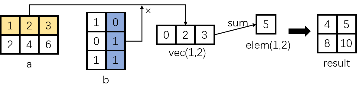
(a) Matrix multiplication

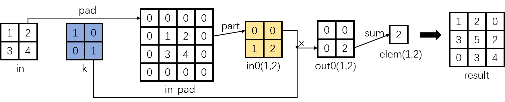
(b) Convolution

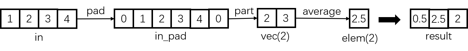
(c) Pooling

Figure 2: Visualizations of ToLang’s representation of three algorithms.

5.4 Representing algorithms with ToLang

We present two classical algorithms in ToLang – Resnet [25] and clustering [26]. For comparison, also we show the original Python code of each algorithm.

5.4.1 Representation for Resnet

We select a basic block in Resnet model [25] as the example. The source code is written in Python with the torch.nn module. Please note that unnecessary details of low-level implementation are removed. Figure 3 is the structure of the basic block from the original paper.

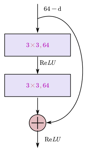
Figure 3: The basic block in Resnet model.

Algorithm 1.1: The basic block in Resnet in Python

⬇

class BasicBlock(nn.Module):

def __init__:

super(BasicBlock, self).__init__()

self.conv1 = conv3x3(in_channel, kernel_size=3, stride=stride,\

padding=1, bias=False)

self.bn1 = nn.BatchNorm2d(out_channel)

self.relu = nn.ReLU(inplace=True)

self.conv2 = conv3x3(out_channel,kernel_size=3, stride=stride,\

padding=1, bias=False)

self.bn2 = nn.BatchNorm2d(out_channel)

self.downsample = downsample

self.stride =stride

#block

def forward(self, x):

residual = x

out = self.conv1(x)

out = self.bn1(out)

out = self.relu(out)

out = self.conv2(out)

out = self.bn2(out)

if self.downsample is not None:

residual = self.downsample(x)

out = out + residual

out = self.relu(out)

return out

Algorithm 1.2: The basic block in Resnet in ToLang
#conv
tol in=[size,size]
in0(i,j)=part(in,[i,j])
out0(i,j)=map(in0(i,j),mul(*,kernel(i,j)),[i,j])
elem(i,j)=reduce(out0(i,j),add,0)
conv(in,kernel):=map(in,elem(i,j),[i,j])
#batch_norm
mean=reduce(in,add,0)
stdvar=sqrt(reduce(map(in,sub(*,mean)),add,0))
bn(in,mean,stdvar):=map(in,sub(*,mean)/stdvar)
#relu
relu(in):=map(in,max(*,0))
#basic_block
residual=in
out=conv.bn.relu.conv.bn(in)
forward(in):=relu(out+residual)

5.4.2 Representation for clustering

We select K-means in classical clustering algorithms [26] as the example. Then, we choose the code from sklearn.cluster, and the following is the very simplified version. We ignore the while-loop as we consider the computation rather than the control flow.

Algorithm 2.1: K-means in clustering algorithm in Python

⬇

class KMeans(object):

#distance

def distance(self, i, center):

diff = self.data[i] - center

return np.sum(np.power(diff, 2))**0.5

#center

def center(self, cluster):

cluster = np.array(cluster)

return …

#main

def cluster(self):

changed = True

while changed: #while-loop

self.clusters = []

for i in range(self.k):

self.clusters.append([])

for i in range(self.capacity):

min_distance = sys.maxsize

center = -1

for j in range(self.k):

distance = self.distance(i,self.centers[j])

if min_distance > distance:

min_distance = distance

center = j

self.clusters[center].append(self.data[i])

newCenters = []

for cluster in self.clusters:

newCenters.append(selfcenter(cluster).tolist())

self.centers = np.array(newCenters)

Algorithm 2.2: K-means in clustering algorithm in ToLang #distance
coordinate=map(data,sqrt(pow(*-center,2)))
dist(data,center):=reduce(coordinate,add,0)
#center
n=|data|
tol centers=[k]
centers(data):=map(centers,rand(n),j)
#main
#loop
tol newcenters=[k]
newcenters=map(reduce(dist(data[i],centers[j]),min,+Inf,i),j)
cluster=newcenters

Operator	Representation	FLOPs	EOPs
ArgMax(t)$\mapsto$axes	reduce(t(i),max,0,iter)/t[1] result=iter	vol(t)	vol(t)
ArgMin(t)$\mapsto$axes	reduce(t(i),min,0,iter)/t[1] result=iter	vol(t)	vol(t)
AveragePool(t,k,p,s)$\mapsto$t	tol result=[(|in|[1]+2*p-k)/s+1] in_pad=[tol[p,|in|],in,tol[p,|in|]] vec(i)=part(in_pad,[(i-1)*s+1,i*s]) elem(i)=reduce(vec(i),add,0)/s result=map(result,elem(i),i)	$\Pi$(—t—[axes]+2*p -k)/s+1)*k	$\Pi$(—t—[axes]+2*p -k)/s+1)*k
BatchNormalization(t,mean,var)$\mapsto$t	map(t,(*-mean)/var)	2*vol(t)	3*vol(t)
Celu(t,alpha)$\mapsto$t	map(t,max(*,0)+min(0,alpha*exp(*/alpha)-1))	-	6*vol(t)
Clip(t,mi,ma)$\mapsto$t	map(t,max(mi,min(*,ma)))	2*vol(t)	2*vol(t)
Concat([t,…])$\mapsto$t	result=[t,...]	0	0
Conv(t,k,p,s)$\mapsto$t	tol result=[(|in|[1]+2*p-k)/s+1] in_pad=[tol[p,|in|],in,tol[p,|in|]] in0(i)=part(in_pad,[(i-1)*s+1,i*s]) out0(i)=map(in0(i),mul(*,k(i)),[i]) elem(i)=reduce(out0(i),add,0) result=map(result,elem(i),[i])	$\Pi$((—t—[axes]+2*p -—k—)/s+1)*2*—k—	$\Pi$((—t—[axes]+2*p -—k—)/s+1)*2*—k—
ConvTranspose(t,shape,p,s)$\mapsto$t	tol result=shape in_pad=[tol[p,|in|],in,tol[p,|in|]] in0(i)=part(in_pad,[(i-1)*s+1,i*s]) result=map(result,in0(i),[i])	$\Pi$((—t—[axes]+2*p -—k—)/s+1)*2*—k—	$\Pi$((—t—[axes]+2*p -—k—)/s+1)*2*—k—
CumSum(t,axes)$\mapsto$t	t0=reshape(t,[axes,-1]) result=reshape(reduce(t0,add,0),|t|)	vol(t)	vol(t)
DepthToSpace(t,blocksize,shape)$\mapsto$t	reshape(t,[shape,blocksize])	0	0
Dropout(t,ratio)$\mapsto$t	map(t,mul(*,rand*ratio))	vol(t)	vol(t)
Elu(t,alpha)$\mapsto$t	map(t,max(*,0)+min(0,alpha*exp(*)-1))	-	5*vol(t)
Expand(t,shape)$\mapsto$t	reshape(t,shape)	0	0
EyeLike(k)$\mapsto$t	tol result=[k,k] result=map(result,eq(iter[1],iter[2]))	0	0
Flatten(t)$\mapsto$t	reshape(t,vol(t))	0	0
Gather(t,axes)$\mapsto$t	map(t,part(*,axes))	0	0
Gemm(t1,t2)$\mapsto$t	tol result=[|a|[1],|b|[2]] vec(i,j)=map(a[i],mul(*,b[*,j])) elem(i,j)=reduce(vec(i,j),add,0) result=map(result,elem(i,j),[i,j])	2*vol(t1)*—t2—[2]	2*vol(t1)*—t2—[2]
Hardmax(t,axes)$\mapsto$t	t0=reshape(t,[axes,-1]) result=reshape(reduce(t0,max,-Inf),|t|)	-	1
HardSigmoid(t,axes)$\mapsto$t	t0=reshape(t,[axes,-1]) result=reshape(reduce(t0,max(0,min(1, (1+*)/2))),|t|)	-	4*vol(t)
HardSwish(t,axes)$\mapsto$t	map(t,min(0,min(*,mul(*,(*+3)/6))))	-	5*vol(t)
Identity(t)$\mapsto$t	result=t	0	0
LeakyRelu(t,alpha)$\mapsto$t	map(t,max(*,mul(alpha,*)))	-	2*vol(t)
LogSoftmax(t,axes)$\mapsto$t	t0=reshape(t,[axes,-1]) result=reshape(map(t0,*/reduce(map(*, exp),add,0),|t|)) result=map(t1,log)	-	2*vol(t)+3
LpNormalization(t,p,axes)$\mapsto$t	t0=reshape(t,[axes,-1]) result=reshape(reduce(map(t,pow(*,p)), add,0),|t|)	3*vol(t)	3*vol(t)
LpPool(t,k,p,s)$\mapsto$t	tol result=[(|in|[1]+2*p-k)/s+1] in_pad=[tol[p,|in|],in,tol[p,|in|]] vec(i)=part(in_pad,[(i-1)*s+1,i*s]) elem(i)=reduce(map(t,pow(*,p)),add,0) result=map(result,elem(i),i)	-	$\Pi$(—t—[axes]+2*p-k) /s+2)*2*k+1
MatMul(t1,t2)$\mapsto$t	tol result=[|a|[1],|b|[2]] vec(i,j)=map(a[i],mul(*,b[*,j])) elem(i,j)=reduce(vec(i,j),add,0) result=map(result,elem(i,j),[i,j])	2*vol(t1)*—t2—[2]	2*vol(t1)*—t2—[2]
MaxPool(t,k,p,s)$\mapsto$t	tol result=[(|in|[1]+2*p-k)/s+1] in_pad=[tol[p,|in|],in,tol[p,|in|]] vec(i)=part(in_pad,[(i-1)*s+1,i*s]) elem(i)=reduce(vec(i),max,0) result=map(result,elem(i),i)	$\Pi$(—t—[axes]+2*p -k)/s+1)*k	$\Pi$(—t—[axes]+2*p -k)/s+1)*k

Table 4: (Part 1/2) ONNX (Open Neural Network Exchange) is an open format built to represent machine learning models. It covers sophisticated computations on tensors and other data formats. This table summarizes how to present the ONNX operators in ToLang. Column 1 is ONNX operators with their parameter formats. Column 2 is a ToLang representation in ToL primitive operators. Column 3 is the FLOPs of the state-of-the-practice algorithms. Column 4 is EOPs derived from the ToL counting rules. Note that “*” refers to an iterator.

Operator	Representation	FLOPs	EOPs
MaxUnpool(t,shape,p,s)$\mapsto$t	tol result=shape in_pad=[tol[p,|in|],in,tol[p,|in|]] vec(i)=[in[i],…(shape[1]/s),in[i]] result=map(result,vec(i),i)	$\Pi$(—t—[axes]+2*p -k)/s+1)*k	$\Pi$(—t—[axes]+2*p -k)/s+1)*k
Mean(t)$\mapsto$t	reduce(t(i),add,0)/|t|	vol(t)	vol(t)
OneHot(n,indices,depth,values)$\mapsto$t	tol result=[n,depth] result=map(tol[n],eq(*,iter))	-	0
Pad(t,p)$\mapsto$t	tol result=[tol[p,|t|],in,tol[p,|t|]]	0	0
PRelu(t,slope)$\mapsto$t	map(t,max(*,mul(slope,*)))	-	2*vol(t)
Range(start,limit,delta)$\mapsto$t	tol in=[limit-start] result=map(in,iter*delta)	vol(t)	vol(t)
ReduceL1(t,axes)$\mapsto$t	t0=reshape(t,[axes,-1]) result=reshape(reduce(t0,add,0),|t|)	2*vol(t)	2*vol(t)
ReduceL2(t,axes)$\mapsto$t	t0=reshape(t,[axes,-1]) result=reshape(map(reduce(map(t0,pow(*,2)), add,0),sqrt),|t|)	2*vol(t)	2*vol(t)
ReduceLogSum(t,axes)$\mapsto$t	t0=reshape(t,[axes,-1]) result=reshape(map(reduce(t0,add,0),log),|t|)	2*vol(t)	2*vol(t)
ReduceLogSumExp(t,axes)$\mapsto$t	t0=reshape(t,[axes,-1]) result=reshape(map(reduce(map(t0,exp), add,0),log),|t|)	3*vol(t)	3*vol(t)
ReduceMax(t,axes)$\mapsto$t	t0=reshape(t,[axes,-1]) result=reshape(reduce(t0,max,-Inf),|t|)	vol(t)	vol(t)
ReduceMean(t,axes)$\mapsto$t	t0=reshape(t,[axes,-1]) result=reshape(map(reduce(t0,add,0), /shape(*)),|t|)	vol(t)	vol(t)
ReduceMin(t,axes)$\mapsto$t	t0=reshape(t,[axes,-1]) result=reshape(reduce(t0,min,+Inf),|t|)	vol(t)	vol(t)
ReduceProd(t,axes)$\mapsto$t	t0=reshape(t,[axes,-1]) result=reshape(reduce(t0,mul,1),|t|)	vol(t)	vol(t)
ReduceSum(t,axes)$\mapsto$t	t0=reshape(t,[axes,-1]) result=reshape(reduce(t0,add,0),|t|)	vol(t)	vol(t)
ReduceSumSquare(t,axes)$\mapsto$t	t0=reshape(t,[axes,-1]) result=reshape(reduce(map(t0,pow(*,2)), add,0),|t|)	2*vol(t)	2*vol(t)
Relu(t)$\mapsto$t	map(t,max(*,0))	-	vol(t)
Reshape(t,sha)$\mapsto$t	reshape(t,sha)	0	0
Selu(t,alpha,gamma)$\mapsto$t	map(t,gamma*max(*,0)+min(0,alpha*exp(*)-1))	-	6*vol(t)
Shape(t)$\mapsto$t	|t|	0	0
Sigmoid(t)$\mapsto$t	map(t,1/(1+exp(-*)))	-	4*vol(t)
Size(t)$\mapsto$ui	vol(t)	0	0
Slice(t,starts,ends,axes,steps)$\mapsto$t	t0=reshape(t,[axes,-1]) result=map(t0,part(*,map(tol[(ends-start) /steps],iter*steps)))	0	0
Softmax(t,axes)$\mapsto$t	t0=reshape(t,[axes,-1]) t1=map(t0,*/reduce(map(*,exp),add,0)) result=reshape(t1,|t|)	-	2*vol(t)+2
Softplus(t)$\mapsto$t	map(t,log(1+exp(*)))	-	3*vol(t)
Softsign(t)$\mapsto$t	map(t,*/(*,sgn(x)))	-	3*vol(t)
SpaceToDepth(t,blocksize)$\mapsto$t	reshape(t,[blocksize])	0	0
Split(t,axes,ui)$\mapsto$[t,…]	t0=reshape(t,[axes,-1]) result=[t0[1],...,t0[|t0|]]	0	0
Sum([t,…])$\mapsto$t	reduce([t,...],add,tol|t|)	vol(t)*n	vol(t)*n
Swish(t)$\mapsto$t	map(t,mul(*,1/(1+exp(-*))))	-	5*vol(t)
ThresholdedRelu(t,th)$\mapsto$t	map(t,mul(gt(*,th),*))	-	2*vol(t)
Transpose(t,axes)$\mapsto$t	reshape(t,swap(|t|,axes))	0	0

Table 5: (Part 2/2) ONNX (Open Neural Network Exchange) is an open format built to represent machine learning models. It covers sophisticated computations on tensors and other data formats. This table summarizes how to present the ONNX operators in ToLang. Column 1 is ONNX operators with their parameter formats. Column 2 is a ToLang representation in ToL primitive operators. Column 3 is the FLOPs of the state-of-the-practice algorithms. Column 4 is EOPs derived from the ToL counting rules. Note that “*” refers to an iterator.

6 ToL has a built-in practical performance indicator

This section shows ToL has a built-in practical performance indicator – elementary operation counts (EOPs) – which is consistent with the widely-used FLOPs [11] metric.

6.1 The definition of elementary operation count (EOPs) and counting rules

ToL is born with a practical performance indicator – elementary operation counts (EOPs), counting how many basic elementary functions are involved in an algorithm. From the definitions in Section 4, we know that the EOPs of an algorithm are definite as they are compositions of ToL operators whose EOPs are also definite according to the rules. The detailed counting rules are as follows.

The EOPs of a function is determined by the number of the basic elementary functions that compose the function. The EOPs of a function is equal to the sum of the EOPs of its basic elementary functions. We consider that the EOPs of each basic elementary function (see Table 2) is one.

Example 13: For variable $x$ and vector $v$ sized $n$, $f(x)=a*x+b$, $g(v)=sqrt(v_{1}^{2}+v_{2}^{2}+\cdots+v_{n}^{2})$. The operation counts are computed as follows.
EOPs$(f(x))=$EOPs$(*)+$EOPs$(+)$=2
EOPs$(g(v))=n*$EOPs$(*)+(n-1)*$EOPs$(+)+$EOPs$(sqrt)$=2*n
This result (2 and 2*n) is consistent with FLOPs count for $f(x)$ and $f(x)$ ($2$ FLOPs and $2n$ FLOPs).

The EOPs of a ToL operator depends on its variable data quantity (vol(<var>)*capacity(<var>)) and the basic elementary functions involved. We define the counting rules of each ToL operator as follows.

• EOPs(single_var)=0

• EOPs(f.g.h....(<var>))=EOPs(f)+EOPs(g)+EOPs(h)+…+EOPs(<var>)
  //rule for composite function

• EOPs(shape)=EOPs(<var>)

• EOPs(dim)=EOPs(<var>)

• EOPs(capacity)=EOPs(<var>)

• EOPs(vol)=EOPs(<var>)

• EOPs(space)=EOPs(<var>)

• EOPs(convert)=EOPs(<var>)

• EOPs(part)=EOPs(<var>)

• EOPs(swap)=EOPs(<var>)

• EOPs(reshape)=EOPs(<var>)

• EOPs(tile)=EOPs(<var>)

• EOPs(map(<var>,<func>,<iter>))=vol(<var>)*capacity(<var>)*EOPs(<func>)+EOPs(
  <var>)

• EOPs(reduce(<var>,<func>,<var_0>,<iter>))=vol(<var>)*capacity(<var>)*EOPs(
  <func>)+EOPs(<var>)+EOPs(<var_0>)

We present matrix multiplication as an example to show how to count the EOPs of an algorithm in detail.

Example 14: Consider EOPs of matrix multiplication represented as result=MatMul(a,b), shown in Section 5.3.1. Suppose a and b are matrices shaped [n,n].
EOPs(result)
=EOPs(map(result,elem(i,j),[i,j]))
=EOPs(result)+|result|*EOPs(elem(i,j))
=n*n*EOPs(reduce(vec(i,j),add,0))
=n*n*(EOPs(vec(i,j))+|vec(i,j)|*EOPs(add))
=n*n*(EOPs(map(a[i],mul(*,b[*,j]))+n*1)
=n*n*(EOPs(a[i])+|a[i]|*EOPs(mul)+n)
=n*n*(n+n)
=2*n*n*n

This result (2*n*n*n) is consistent with the FLOPs count for matrix multiplication ($2n^{3}$ FLOPs).

6.2 Evaluations on the ONNX operators

This subsection uses the ONNX [10] operators as an example to show that the EOPs metric is consistent with the FLOPs in a complex application scenario like AI or big data.

According to the counting rules defined in the last section, we compute the EOPs and the FLOPs (the third and fourth columns) of ONNX operators in Table 4 and 5. We obtain the FLOPs after analyzing the state-of-the-practice implementations of the ONNX operators and calculate the EOPs according to the counting rules defined in the last section. The comparisons show that EOPs are consistent with FLOPs within a minimal error range. This evaluation further shows that ToLang has a built-in realistic performance indicator.

7 Conclusion

This article presented a unified computation model with a generalized expression ability: ToL. ToL includes a unified data abstraction – Tensor of List, and a unified computation model based on Tensor of List. ToL introduces five atomic computations that can represent any elementary computation by finite compositions, ensured with strict formal proof. Based on ToL, we designed a pure-functional language – ToLang. ToLang provides a concise set of primitive operators that can be used to program complex big data and AI algorithms. The evaluations showed ToL has generalized expression ability and a built-in performance indicator, born with a strictly defined computation metric – elementary operation count (EOPs), consistent with FLOPs within a small error range.

References

- [1] A. M. Turing, “Turing, a.m.: On computable numbers, with an application to the entscheidungs problem. proc. lond. math. soc. ser. 2 42, 230-265,” Proceedings of the London Mathematical Society, vol. 42, no. 1, pp. 230–265, 1937.
- [2] A. Adamatzky, Game of life cellular automata, vol. 1. Springer, 2010.
- [3] C. G. Langton, “Studying artificial life with cellular automata,” Physica D: Nonlinear Phenomena, vol. 22, no. 1-3, pp. 120–149, 1986.
- [4] H. P. Barendregt, “The lambda calculus”,” Studies in Logic, vol. 3, no. 2, pp. 181–215, 1988.
- [5] A. V. Aho and J. D. Ullman, “Universality of data retrieval languages,” in Proceedings of the 6th ACM SIGACT-SIGPLAN symposium on Principles of programming languages, pp. 110–119, 1979.
- [6] ISO, “Information technology — database languages — sql.” [EB/OL]. https://www.iso.org/standard/63555.html Accessed November 1, 2022.
- [7] F. Geerts, T. Muñoz, C. Riveros, and D. Vrgoč, “Expressive power of linear algebra query languages,” in Proceedings of the 40th ACM SIGMOD-SIGACT-SIGAI Symposium on Principles of Database Systems, pp. 342–354, 2021.
- [8] M. Abadi, P. Barham, J. Chen, Z. Chen, and X. Zhang, “Tensorflow: A system for large-scale machine learning,” USENIX Association, 2016.
- [9] A. Paszke, S. Gross, F. Massa, A. Lerer, and S. Chintala, “Pytorch: An imperative style, high-performance deep learning library,” 2019.
- [10] O. Authors, “Open neural network exchanges.” [EB/OL]. https://onnx.ai/ Accessed November 1, 2022.
- [11] J. J. Dongarra, P. Luszczek, and A. Petitet, “The linpack benchmark: past, present and future,” Concurrency & Computation Practice & Experience, vol. 15, no. 9, pp. 803–820, 2010.
- [12] H. Vollmer, Introduction to circuit complexity: a uniform approach. Springer Science & Business Media, 1999.
- [13] A. M. Turing, “Computability and -definability,” The Journal of Symbolic Logic, vol. 2, no. 4, pp. 153–163, 1937.
- [14] M. Kline, Mathematical Thought from Ancient to Modern Times: Volume 2, vol. 2. Oxford university press, 1990.
- [15] E. F. Codd, “A relational model of data for large shared data banks,” Communications of the ACM, vol. 13, no. 6, pp. 377–387, 1970.
- [16] K. Asanovic, R. Bodik, B. C. Catanzaro, J. J. Gebis, P. Husbands, K. Keutzer, D. A. Patterson, W. L. Plishker, J. Shalf, and S. W. Williams, “The landscape of parallel computing research: A view from berkeley,” 2006.
- [17] W. Gao, J. Zhan, L. Wang, C. Luo, D. Zheng, F. Tang, B. Xie, C. Zheng, X. Wen, and X. He, “Data motifs: A lens towards fully understanding big data and ai workloads,” in Proceedings of the 27th International Conference on Parallel Architectures and Compilation Techniques, pp. 1–14, 2018.
- [18] J. Melton and A. R. Simon, Understanding the new SQL: a complete guide. Morgan Kaufmann, 1993.
- [19] R. Brijder, F. Geerts, J. V. d. Bussche, and T. Weerwag, “On the expressive power of query languages for matrices,” arXiv preprint arXiv:1709.08359, 2017.
- [20] P. Hudak and J. H. Fasel, “A gentle introduction to haskell,” ACM Sigplan Notices, vol. 27, no. 5, pp. 1–52, 1992.
- [21] J. Liouville, Premier mémoire sur la détermination des intégrales dont la valeur est algébrique. Impr. Royale, 1833.
- [22] A. Shpilka and A. Yehudayoff, “Arithmetic circuits: a survey of recent results and open questions,” Foundations & Trends in Theoretical Computer ence, vol. 5, no. 3-4, pp. 207–388, 2010.
- [23] T. H. Cormen, C. E. Leiserson, R. L. Rivest, and C. Stein, Introduction to algorithms. MIT press, 2022.
- [24] T. E. Oliphant, A guide to NumPy, vol. 1. Trelgol Publishing USA, 2006.
- [25] K. He, X. Zhang, S. Ren, and J. Sun, “Deep residual learning for image recognition,” in Proceedings of the IEEE conference on computer vision and pattern recognition, pp. 770–778, 2016.
- [26] K. Krishna and M. N. Murty, “Genetic k-means algorithm,” IEEE Transactions on Systems, Man, and Cybernetics, Part B (Cybernetics), vol. 29, no. 3, pp. 433–439, 1999.