Anharmonic lattice dynamics via the special displacement method

Abstract

On the basis of the self-consistent phonon theory and the special displacement method, we develop an approach for the treatment of anharmonicity in solids. We show that this approach enables the efficient calculation of temperature-dependent anharmonic phonon dispersions, requiring very few steps to achieve minimization of the system’s free energy. We demonstrate this methodology in the regime of strongly anharmonic materials which exhibit a multi-well potential energy surface, like cubic SrTiO₃, CsPbBr₃, CsPbI₃, CsSnI₃, and Zr. Our results are in good agreement with experiments and previous first-principles studies relying on stochastic nonperturbative and molecular dynamics simulations. We achieve a very robust workflow by using harmonic phonons of the polymorphous ground state as the starting point and an iterative mixing scheme of the dynamical matrix. We also suggest that the phonons of the polymorphous ground state might provide an excellent starting approximation to explore anharmonicity. Given the simplicity, efficiency, and stability of the present treatment to anharmonicity, it is especially suitable for use with any electronic structure code and for investigating electron-phonon couplings in strongly anharmonic systems.

I Introduction

Incorporating anharmonic lattice dynamics in first-principles calculations of solids has been a central topic of research over the last fifteen years owing to their importance in describing accurately vibrational, transport, and optoelectronic properties at finite temperatures [1, 2, 3, 4, 5, 6, 7, 8, 9]. Anharmonicity in solids can broadly be classified by inspecting the potential energy surface (PES), representing the variation of the system’s potential energy with respect to the positions of the nuclei (Fig. 1). When variations in the potential energy can be fully or nearly described by a parabola [Figs. 1(a) and (b)], the system is classified as harmonic or weakly anharmonic. In these cases one can exploit the standard harmonic approximation to efficiently evaluate the vibrational (phonon) spectra by means of density functional perturbation theory (DFPT) [10] or the frozen-phonon method (FPM) [11]. If, however, the PES is distinctly different from a parabola, the system can be classified as anharmonic [Figs. 1(c) and (d)] and the standard harmonic approximation breaks down, leading to instabilities (imaginary frequencies) in the phonon spectrum. In this case, one needs to resort to a higher level theory.

Figure 1: Schematic illustration of PES representing various levels of anharmonicity: (a) harmonic, (b) weakly anharmonic, (c) anharmonic with a single well, and (d) anharmonic with a double well PES. Orange curves represent the true potential and blue curves are harmonic fits around static equilibrium positions of the nuclei $\tau_{\rm eq}$.

The self-consistent phonon (SCP) theory [12, 13, 14] forms the basis of current state-of-the-art methodologies employed for the treatment of lattice anharmonicity. These methodologies rely on (i) nonperturbative stochastic approaches that obtain self-consistency in the phonon spectrum [15, 16, 17, 18], or minimize directly the system’s free energy [19, 20, 21, 22], (ii) ab initio molecular dynamics [23, 24, 25] (aiMD) for the extraction of an effective matrix of interatomic force constants (IFCs) by least-squares fitting, and (iii) the explicit computation of higher-order IFCs [4, 26, 27, 28]. The success of (i)-(iii) has been demonstrated, among others, in calculations of temperature-dependent (anharmonic) phonon dispersions, free energies, phase diagrams, lattice conductivities, specific heats, and phonon-phonon scattering rates [15, 16, 17, 18, 19, 20, 21, 23, 24, 25, 26, 29, 27, 28].

In parallel with the development of efficient computational methods to treat anharmonicity in solids, the field of electron-phonon interactions from first principles [30] is growing tremendously popular [31, 32, 33, 34, 35, 36]. Therefore, interfacing the rather challenging calculations of electron-phonon properties [37, 38, 39] with practical calculations of anharmonic phonons is of paramount importance. The increasing importance and popularity of these calculations call for the development of simple and efficient approaches to anharmonicity that can be applied straightforwardly by end-users on top of any electronic structure code.

In this work we focus towards this perspective and develop a nonperturbative first-principles approach to anharmonicity that relies on the combination of the SCP theory and the special displacement method [40, 41]. We demonstrate that special displacements in small supercells can be employed to capture very efficiently the anharmonicity in the IFCs via the computation of an effective PES. In particular, we show that self-consistency in the phonon spectra can be achieved in very few steps using a single thermally distorted configuration at each iteration and taking the polymorphous ground state network [42] as the starting point. The overall convergence performance is enhanced by an iterative mixing scheme. Our suggested workflow is very simple as it relies on basic first-principles tools such as the FPM or DFPT. We name our approach A-SDM, standing for anharmonicity (A) using the special displacement method (SDM). In order to demonstrate the A-SDM, we report anharmonic phonons of the cubic perovskites SrTiO₃, CsPbBr₃, CsPbI₃, and CsSnI₃, tetragonal SrTiO₃, as well as body-centered cubic (bcc) Zr. Our results compare well with experiments and previous calculations based on stochastic, aiMD, or other variational approaches that rely on truncated Taylor expansions of the PES.

The paper is organized as follows. In Sec. II we describe the theoretical framework of lattice dynamics and our methodology to anharmonicity, putting together the concepts underpinning SCP and SDM theories. In Sec. III we outline the main procedure of the A-SDM and show its capability in computing temperature-dependent phonon spectra of cubic SrTiO₃, CsPbBr₃, CsPbI₃, CsSnI₃, and Zr. Section IV describes improvements related to the self-consistent scheme and reports all computational details. Our conclusions and outlook are provided in Sec. V.

II Theory

Here we describe the theoretical framework underpinning the A-SDM to deal with lattice anharmonicity in crystals. Our approach is conceptually similar to other SCP methods developed in the past [1, 5, 7]; the aspect introduced here is that special displacements can be employed to accelerate considerably the sampling of the nuclei configuration space.

II.1 Lattice dynamics

To describe lattice dynamics we resort to supercell periodic boundary conditions and, at first, to the standard harmonic approximation. Hence we take the Taylor expansion of the PES up to second order in atomic displacements to write:

$$U^{\{\tau\}} = U_{0}+\frac{1}{2}\sum_{\begin{subarray}{c}p\kappa\alpha\\ p^{\prime}\kappa^{\prime}\alpha^{\prime}\end{subarray}}\frac{\partial^{2}U}{\partial\tau_{p\kappa\alpha}\partial\tau_{p^{\prime}\kappa^{\prime}\alpha^{\prime}}}\Delta\tau_{p\kappa\alpha}\Delta\tau_{p^{\prime}\kappa^{\prime}\alpha^{\prime}}.$$ (1)

Here $U_{0}$ is a local extrema of the PES with the atoms at their static equilibrium positions $\tau_{p\kappa\alpha}$ where $p$, $\kappa$, and $\alpha$ indices represent the unit cell (position vector ${\bf R}_{p}$), the atom (position vector $\boldsymbol{\tau}_{\kappa}$), and the Cartesian component, respectively. The displacements of the atoms away from their static equilibrium positions are denoted as $\Delta\tau_{p\kappa\alpha}$.

To obtain the phonon spectrum one needs to evaluate the dynamical matrix for lattice vibrations obtained as the Fourier transform of the IFCs [43]:

$$D_{\kappa\alpha,\kappa^{\prime}\alpha^{\prime}}({\bf q})=\sum_{p^{\prime}}\frac{C_{0\kappa\alpha,p^{\prime}\kappa^{\prime}\alpha^{\prime}}}{\sqrt{M_{\kappa}M_{\kappa^{\prime}}}}e^{i{\bf q}\cdot{\bf R}_{p^{\prime}}}e^{i{\bf q}\cdot({\boldsymbol{\tau}}_{\kappa^{\prime}}-{\boldsymbol{\tau}}_{\kappa})},$$ (2)

where ${\bf q}$ is a wavevector of the reciprocal space, the IFCs matrix elements are defined as $C_{p\kappa\alpha,p^{\prime}\kappa^{\prime}\alpha^{\prime}}=\partial^{2}U/\partial\tau_{p\kappa\alpha}\partial\tau_{p^{\prime}\kappa^{\prime}\alpha^{\prime}}$, and $M_{\kappa}$ represents the atomic mass. The subscript $0$ is used to indicate that IFCs are calculated with respect to a reference unit cell which is invariant upon translation. For high-symmetry systems, the IFCs entering Eq. (2) should remain invariant under the crystal’s symmetry operations $\{{\bf S}|{\bf v}(S)+{\bf R}_{m}\}$, where ${\bf S}$ represents a rotation (proper or improper) and ${\bf v}(S)$ is a fractional translation associated with ${\bf S}$. That is, if the position vectors of two atoms are related by [44]

$$\boldsymbol{\tau}_{PK}={\bf S}\,\boldsymbol{\tau}_{p\kappa}+{\bf v}(S)+{\bf R}_{m},$$ (3)

then the following relationship should hold for the matrix elements of the IFCs

$$C_{PK\alpha,P^{\prime}K^{\prime}\alpha^{\prime}}=\sum_{\beta\beta^{\prime}}S_{\alpha\beta}S_{\alpha^{\prime}\beta^{\prime}}C_{p\kappa\beta,p^{\prime}\kappa^{\prime}\beta^{\prime}}.$$ (4)

A great advantage of using symmetry operations is that the computation of the full dynamical matrix can be obtained by applying finite displacements to a few atoms in the unit cell.

For polar semiconductors, the long-range dipole-dipole (dd) interactions, induced by collective ionic displacements, are treated by employing the standard non-analytical correction in the limit ${\bf q}\rightarrow 0$. This correction to the dynamical matrix is given by [45]:

$$D^{\rm dd}_{\kappa\alpha,\kappa^{\prime}\alpha^{\prime}}({\bf q}\rightarrow 0)=$$ (5)

$$\frac{1}{\sqrt{M_{\kappa}M_{\kappa^{\prime}}}}\frac{4\pi e^{2}}{\Omega}\frac{\sum_{\beta}q_{\beta}Z^{*}_{\kappa,\beta\alpha}\sum_{\beta^{\prime}}q_{\beta^{\prime}}Z^{*}_{\kappa^{\prime},\beta^{\prime}\alpha^{\prime}}}{\sum_{\beta\beta^{\prime}}q_{\beta}\epsilon^{\infty}_{\beta\beta^{\prime}}q_{\beta^{\prime}}},$$

where $e$ is the electron charge, $\Omega$ represents the volume of the unit cell, $Z^{*}_{\kappa,\beta\alpha}$ are the matrix elements of the Born-effective charge tensor, and $\epsilon^{\infty}_{\beta\beta^{\prime}}$ are the matrix elements of the high-frequency dielectric constant. This term leads to the splitting between the longitudinal optical (LO) and transverse optical (TO) modes at the zone-center. At general ${\bf q}$ points, the long-range dipole-dipole effect can be accounted for using the linear response or mixed space approaches described in Refs. [45] and [46], respectively.

Having obtained the components of the dynamical matrix, the phonon frequencies $\omega_{{\bf q}\nu}$ and polarization vectors $e_{\kappa\alpha,\nu}({\bf q})$ corresponding to wavevector ${\bf q}$ and mode $\nu$ are determined by solving the eigenvalue equation:

$$\sum_{\kappa^{\prime}\alpha^{\prime}}D_{\kappa\alpha,\kappa^{\prime}\alpha^{\prime}}({\bf q})e_{\kappa^{\prime}\alpha^{\prime},\nu}({\bf q})=\omega^{2}_{{\bf q}\nu}e_{\kappa\alpha,\nu}({\bf q}).$$ (6)

The frequencies $\omega_{{\bf q}\nu}$ define the phonon dispersion in the fundamental Brillouin zone of the crystal’s unit cell.

Figure 2: Schematic illustration of a harmonic (a) and a double-well anharmonic (b) PES. Orange and black curves represent the true and effective potentials. Green and red curves are harmonic fits around saddle points of the PES defined by static equilibrium positions of the nuclei. Black dashed line represents the solution of the nuclear Schrödinger equation. The local maximum and minima of the PES in (b) correspond to the monomorphous (high-symmetry) and polymorphous configurations, respectively.

II.2 Treatment of anharmonicity via the special displacement method: A-SDM

When the displacements are small, the atoms remain near the bottom of the PES well and the harmonic approximation to lattice dynamics is appropriate for solving the nuclear Schrödinger equation [Fig. 2(a)]. In the case of a double well potential, a harmonic approximation at the local maximum is still possible but fails completely to describe the free energy of the system [green curve in Fig. 2(b)]. Instead, one can apply the harmonic approximation in one of the two PES wells, corresponding to the system’s ground state, and obtain a reasonable estimate [red curve in Fig. 2(b)]. However, there is no direct indication how accurate this estimate is, until the actual solution of the nuclear Schrödinger equation or the system’s free energy are obtained [47]. The most popular approach to capture anharmonicity is to find an effective harmonic potential whose solution matches the one of the true PES [black line in Fig. 2(b)].

To account for anharmonic effects in the lattice dynamics we base our approach on the SCP theory. The merit of this theory is that the true potential (e.g. double well) can be replaced by an effective temperature-dependent harmonic potential, provided this effective potential minimizes the free energy. The problem involved is to determine, essentially, the temperature-dependent matrix of IFCs

$$C_{p\kappa\alpha,p^{\prime}\kappa^{\prime}\alpha^{\prime}}(T)=\Braket{\frac{\partial^{2}U^{\{\tau\}}}{\partial\tau_{p\kappa\alpha}\partial\tau_{p^{\prime}\kappa^{\prime}\alpha^{\prime}}}}_{T},$$ (7)

iteratively until self-consistency is reached. The notation $\braket{.}_{T}$ represents the ensemble thermal average which acts as the trace over the complete set of quantum harmonic oscillators weighted by the standard Boltzmann factor at temperature $T$ and normalized by the canonical partition function. For completeness, we provide the proof of Eq. (7) in Appendix A. The thermal average can be expressed as a multivariate Gaussian integral of the following form [41]:

$$C_{p\kappa\alpha,p^{\prime}\kappa^{\prime}\alpha^{\prime}}(T)=\prod_{{\bf q}\nu}\!\int\!\frac{dz_{{\bf q}\nu}}{u_{{\bf q}\nu}\sqrt{2\pi}}e^{-\frac{|z_{{\bf q}\nu}|^{2}}{2u^{2}_{{\bf q}\nu}}}\frac{\partial^{2}U^{\{\tau\}}}{\partial\tau_{p\kappa\alpha}\partial\tau_{p^{\prime}\kappa^{\prime}\alpha^{\prime}}}.$$

Here $z_{{\bf q}\nu}$ are the normal coordinates and $u^{2}_{{\bf q}\nu}$ is the mode-resolved mean-square displacement of the nuclei given by:

$$u^{2}_{{{\bf q}}\nu}(T)=\frac{\hbar}{2M_{0}\omega_{{{\bf q}}\nu}}[2n_{{{\bf q}}\nu}(T)+1],$$ (9)

where $M_{0}$ is the proton mass and $n_{{\bf q}\nu}(T)$ is the Bose-Einstein occupation of the phonon $\omega_{{\bf q}\nu}$.

At each iteration the thermal average can be evaluated stochastically using Monte Carlo approaches [19, 48, 20, 18]. In these approaches, displaced nuclei configurations at each temperature are generated by drawing normal coordinates from the multivariate normal distribution to evaluate $C_{p\kappa\alpha,p^{\prime}\kappa^{\prime}\alpha^{\prime}}(T)$ and, hence, the dynamical matrix. Minimization of the system’s free energy is achieved when self-consistency with respect to IFCs and thus phonon frequencies and eigenvectors is obtained. This aspect has been demonstrated and discussed in Ref. [18]. The free energy is defined as $F=U-TS$, where U is the total energy and $S$ the vibrational entropy, and can be expressed as [43, 5]:

$$F(T) = \braket{U}_{T}-\frac{M_{0}}{2}\sum_{{\bf q}\nu}\omega^{2}_{{\bf q}\nu}u^{2}_{{{\bf q}}\nu}(T)$$

$$+ \sum_{{\bf q}\nu}\bigg{[}\frac{\hbar\omega_{{\bf q}\nu}}{2}-k_{\rm B}T\,{\rm ln}[1+n_{{\bf q}\nu}(T)]\bigg{]}.$$

Here, $\braket{U}_{T}$ is the thermal average of the true PES taken with respect to the eigenstates of the effective harmonic Hamiltonian, the term $M_{0}/2\sum_{{\bf q}\nu}\omega^{2}_{{\bf q}\nu}u^{2}_{{{\bf q}}\nu}(T)$ is the vibrational energy of the effective harmonic Hamiltonian, and $k_{\rm B}$ is the Boltzmann constant.

To evaluate Eq. (7) more efficiently we propose to replace the cumbersome stochastic sampling for the calculation of $C_{p\kappa\alpha,p^{\prime}\kappa^{\prime}\alpha^{\prime}}(T)$ with SDM [40, 41]. For this purpose it suffices to set the nuclei of the system at coordinates defined by Zacharias-Giustino (ZG) displacements and calculate

$$C_{p\kappa\alpha,p^{\prime}\kappa^{\prime}\alpha^{\prime}}(T)\simeq\frac{\partial^{2}U^{\{\tau^{\rm ZG}\}}}{\partial\tau_{p\kappa\alpha}\partial\tau_{p^{\prime}\kappa^{\prime}\alpha^{\prime}}}.$$ (11)

Here the coordinates are defined as $\tau^{\rm ZG}=\tau+\Delta\tau^{\rm ZG}$, where $\Delta\tau^{\rm ZG}$ represent the ZG displacements. These are given by [41]:

$$\Delta\tau^{\rm ZG}_{p\kappa\alpha}=\sqrt{\frac{M_{0}}{N_{p}M_{\kappa}}}2\,\!\sum_{{\bf q}\nu}\!S_{{\bf q}\nu}u_{{\bf q}\nu}\,{\rm Re}\Big{[}e^{i{\bf q}\cdot{\bf R}_{p}}e_{\kappa\alpha,\nu}({\bf q})\Big{]},$$ (12)

where the notation $N_{p}$ stands for the number of unit cells comprising the supercell. The quantities $S_{{\bf q}\nu}$ represent an optimal choice of signs ($\pm 1$) determined by the EPW/ZG module [39] so as to ensure that the resulting ZG configuration at temperature $T$ yields the best possible approximation to Eq. (II.2). We note that ZG displacements have been originally designed for the one-shot evaluation of electron-phonon effects using supercells. In this work we expand this idea for the efficient treatment of anharmonic dynamics. In fact, ZG displacements are perfectly suited for describing an effective potential since one of the premises of the SDM theory requires vanishing IFCs between atoms in distant unit cells (see Eq. (45) of Ref. [41]).

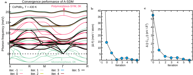
Figure 3: (a) Convergence performance of the A-SDM in computing the phonon dispersion of cubic CsPbBr₃ at $T=430$ K. The calculations refer to 2$\times$2$\times$2 supercells using the experimental lattice constant [49] of 5.847 Å. IFCs at each iteration were evaluated by finite differences including corrections due to long-range dipole-dipole interactions. Iteration -1 and 0 correspond to the phonons calculated for the high-symmetry (monomorphous) and ground state (polymorphous) structures, respectively. The dispersion of the polymorphous structure is obtained after applying the crystal’s symmetry (SYM) operations on the IFCs [Eq. (4)]. (b) Differential free energy ($\Delta F$) as a function of the number of iterations. $\Delta F$ is evaluated as the difference between the free energy [Eq. (II.2)] of the current and the last ZG configuration. (c) Differential Frobenius norm of the leading IFCs ($\Delta||C_{1,1}||$) as a function of the number of iterations. $\Delta||C_{1,1}||$ is evaluated as the difference between $||C_{1,1}||$ [Eq. (16)] of the current and the last IFCs.

The straightforward evaluation of Eq. (11) involves performing FPM or DFPT on a thermally displaced configuration in the same fashion with standard phonon calculations of harmonic systems. However, the “brute force” computation of $C_{p\kappa\alpha,p^{\prime}\kappa^{\prime}\alpha^{\prime}}(T)$ by DFPT or FPM becomes prohibitively expensive with the supercell size. Instead, one can calculate $C_{p\kappa\alpha,p^{\prime}\kappa^{\prime}\alpha^{\prime}}(T)$ at each iteration much more efficiently by relying only on the Hellman-Feynman forces, $F_{p\kappa\alpha}$, acting on the nuclei contained in a ZG supercell through the following relationship [16, 21]:

$$C_{p\kappa\alpha,p^{\prime}\kappa^{\prime}\alpha^{\prime}}(T) \simeq \sum_{p^{\prime\prime}\kappa^{\prime\prime}\alpha^{\prime\prime}}\frac{\sqrt{M_{\kappa^{\prime}}M_{\kappa^{\prime\prime}}}}{M_{0}}\Delta\tau^{\rm ZG}_{p^{\prime\prime}\kappa^{\prime\prime}\alpha^{\prime\prime}}F_{p\kappa\alpha}^{\{\tau^{\rm ZG}\}}$$ (13)

$$\times \sum_{\nu}\frac{e_{\kappa^{\prime}\alpha^{\prime},\nu}({\bf 0})e_{\kappa^{\prime\prime}\alpha^{\prime\prime},\nu}({\bf 0})}{u^{2}_{{\bf 0}\nu}}.$$

Here all quantities refer to supercell calculations (${\bf q}={\bf 0}$) and both $e_{\kappa\alpha,\nu}({\bf 0})$ and $u^{2}_{{\bf 0}\nu}$ are as obtained in the previous iteration. The derivation of Eq. (13) proceeds by (i) starting from $C_{p\kappa\alpha,p^{\prime}\kappa^{\prime}\alpha^{\prime}}(T)=\Braket{\partial F_{p\kappa\alpha}/\partial\tau_{p^{\prime}\kappa^{\prime}\alpha^{\prime}}}_{T}$, (ii) expressing the derivative with respect to atomic displacements into its normal coordinate representation [41], (iii) writing the thermal average as in Eq. (II.2), (iv) making use of integration by parts, and (v) replacing the thermal average with its ZG analogue.

II.3 Applications of the A-SDM beyond the SCP theory for symmetric phases

It should be pointed out that the SDM can also be exploited for the efficient calculation of the generalization of Eq. (7) for higher-order force constants, or in other words, the computation of the Gaussian integral appearing in Eq. (II.2) for derivatives of the potential of any degree. The calculation of thermal averages of higher-order force constants should be within reach. If successful, this additional information will be useful to investigate second-order phase transitions within Landau’s framework [21] in future work. Furthermore, when nuclei are not enforced to respect crystal symmetries, or occupy general Wyckoff positions (i.e. can be treated as free parameters), it is also desirable to minimize the free energy with respect to the internal coordinates. This requires:

$$\Braket{\frac{\partial U}{\partial\tau_{p\kappa\alpha}}}_{T}=0.$$ (14)

The solution of the above equation can be obtained, for example, using the Newton–Raphson method [16] so that at each iteration we update the equilibrium positions through the relationship:

$$\tau^{\rm new}_{p\kappa\alpha}=\tau_{p\kappa\alpha}+C^{-1}_{p\kappa\alpha,p\kappa\alpha}\,F_{p\kappa\alpha}^{\{\tau^{\rm ZG}\}}$$ (15)

where $C^{-1}_{p\kappa\alpha,p\kappa\alpha}$ is the inverse of IFCs matrix evaluated through Eq. (11). We note that there exist other approaches for solving Eq. (14) that rely on the conjugate gradient method [19]. Also in this case, the SDM can be proven useful. In the present manuscript, we mostly study high-symmetry systems characterized by special Wyckoff positions and therefore Eq. (14) is respected by construction so that $\tau^{\rm new}_{p\kappa\alpha}=\tau_{p\kappa\alpha}$ at each iteration.

III Main procedure and Results

III.1 Main procedure of the A-SDM

We stress that the present variant of the SCP theory requires only one thermal supercell configuration at each iteration $j$ and avoids encountering instabilities in the phonon spectra at any intermediate step; this is consistent with the fact that the SCP theory [Eq. (7)] is designed to work only with positive definite IFCs. In the following, we outline the workflow of the proposed technique:

1. Obtain the ground state polymorphous configuration of the system in a supercell by tight optimization of the nuclear coordinates, keeping the lattice constants fixed.

2. Compute the initial matrix of IFCs, ${\bf C}_{0}$, using the polymorphous configuration by means of DFPT or FPM and apply the crystal’s symmetries [Eq. (4)].

3. Generate the dynamical matrix [Eq. (2)] and obtain the phonons by diagonalization [Eq. (6)].

4. Generate $\Delta\tau^{\rm ZG}$ [Eq. (12)] for temperature $T$ using the computed phonons and displace the nuclei from their high symmetry positions in a supercell. This step is performed with the ZG.x code of EPW [39].

5. Compute ${\bf C}_{j}(T)$ using the ZG configuration [either with Eq. (11) or Eq. (13)].

6. Apply the crystal’s symmetries to ${\bf C}_{j}(T)$ [Eq. (4)].

7. Apply linear mixing ${\bf C}_{j}\,=\,\beta\,{\bf C}_{j}+(1-\beta)\,{\bf C}_{j-1}$, where $\beta$ is the mixing factor between 0.2 and 0.7, and compute the phonons as in step 3.

8. Repeat steps 4-7 until self-consistency in the IFCs [Eq. (7)], and therefore, in phonon frequencies and eigenvectors is reached.

9. If convergence with respect to supercell size is sought, go to step 4 and generate a ZG configuration in a larger supercell using the self-consistent phonons obtained in step 8.

Figure 4: Harmonic phonon dispersions of (a) cubic SrTiO₃ and (b) tetragonal SrTiO₃ calculated using the monomorphous (green) and polymorphous (red) structures. Results were obtained using 2$\times$2$\times$2 supercells (40 atoms for the cubic and 80 for the tetragonal phase), the PBEsol approximation, and including long-range dipole-dipole interactions.

Let us remark that in the present procedure both phonon frequencies and eigenvectors are updated iteratively. However, a complete self-consistent phonon scheme also allows to explore new thermal equilibrium positions [Eq. (15)] at each step, which play a key role in describing structural phase transitions at critical temperatures [21]. Here, we limit our calculations to temperatures away from critical points, and mostly consider systems for which the nuclei remain at their special Wyckoff positions.

We note that for materials with a multi-well PES, their ground state structures in step 1 are obtained by initially displacing the atoms in a supercell along the soft modes computed for the high-symmetry structure and then performing a tight relaxation of the atomic coordinates with the lattice constants fixed. More details are provided in Sec. IV.2. Following the definitions made in Ref. [42], we refer to the high-symmetry and ground state structures as the monomorphous and polymorphous networks, respectively.

In Fig. 3(a) we demonstrate the performance of the A-SDM for calculating the phonon dispersion of cubic CsPbBr₃ at $T=430$ K. Iteration -1 refers to the phonons computed for the monomorphous structure, featuring large instabilities. Iteration 0 represents the symmetrized phonon dispersion of the polymorphous structure computed by performing steps 1-3. We indicate this phonon dispersion as Polymorphous-SYM for the rest of the manuscript. The phonon dispersions from iteration 1 to 5 are evaluated by repeating steps 4-7 using a mixing parameter $\beta=0.5$ until self-consistency is achieved. Impressively, our results show that the A-SDM exhibits an outstanding efficiency requiring maximum 3-4 configurations for self-consistency in the phonon spectra. This can also be seen by inspecting the variation of the differential free energy, using Eq. (II.2), with respect to the number of iterations, shown in Fig. 3(b). We emphasize that even the first iteration (grey line) provides reasonable results, being very close to the converged dispersion. We also stress that owing to the linear mixing scheme (step 7), none of the iterations suffer from phonon spectra with instabilities. This feature of our technique constitutes an advantage over previous approaches [16, 18]. In Sec. IV.1, we illustrate the validity of the iterative mixing scheme.

As a sanity check, we also calculated the Frobenius norm of the leading components of the IFCs matrix as:

$$||C_{1,1}||=\sum_{\kappa}||{\bf C}_{1\kappa,1\kappa}||,$$ (16)

where we set the unit cell index $p=1$. As shown in Fig. 3(c), the convergence behavior of $||C_{1,1}||$ is similar to that of the free energy. We propose that computing $||{\bf C}_{1\kappa,1\kappa}||$ for small ZG supercells can be advantageous over relying solely on numerical convergence of the free energy. This is because the error involved in the evaluation of $\braket{U}_{T}$, entering the expression in Eq. (II.2), might slow down convergence for small ZG supercells.

III.2 SrTiO3

In this section we demonstrate our methodology by taking as a test case the phonon dispersion of SrTiO₃ for which extensive theoretical and experimental data exist in the literature [50, 51, 52, 53, 26, 54, 55, 28, 18, 56].

Figure 5: (a) Temperature-dependent phonon dispersion of polymorphous cubic SrTiO₃ calculated using the quasiharmonic approximation (QHA) for $T=0$ K (red), $300$ K (blue), and $500$ K (black). Thermal lattice expansion was taken into account using experimental data from Ref. [57]. The phonon dispersions of the polymorphous structures were evaluated after applying the crystal symmetries (SYM) to the IFCs. (b) Phonon frequency of the zone-center TO modes of cubic SrTiO₃ as a function of temperature. Red diamonds correspond to our calculations in the QHA using the cubic polymorphous structure. Discs and solid lines represent data from Ref. [26] obtained using the TDEP and SCP-TE methods, respectively. Squares depict the results of Ref. [56] evaluated within the SSCHA. Experimental data, shown as triangles, are from Refs. [51] and [53]. (c) Temperature-dependent phonon dispersion of cubic SrTiO₃ calculated using the A-SDM for $T=0$ K (orange), $T=300$ K (blue), $500$ K (green), and $900$ K (black). The symmetrized phonon dispersion of polymorphous cubic SrTiO₃ at 0 K (red) is shown for comparison. (d) Temperature-dependent phonon dispersion of tetragonal SrTiO₃ calculated using the A-SDM for $T=0$ K (black). The symmetrized phonon dispersion of polymorphous tetragonal SrTiO₃ at 0 K (red) is shown for comparison. (e) As in (b) but now blue diamonds represent calculations using the A-SDM. Green diamonds are for the TO1 frequency calculated for the tetragonal structure using the A-SDM. The vertical dashed line at $T=105$ K indicates the phase transition temperature. All calculations refer to 2$\times$2$\times$2 supercells of cubic or tetragonal SrTiO₃ and are performed within the PBEsol approximation. Dispersions in (a), (c), and (d) include long-range corrections.

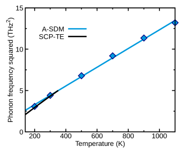
Figure 6: Temperature dependence of the squared frequency of the AFD soft mode at R-point calculated with the A-SDM (blue diamonds) and SCP-TE (black line) approaches using a 2$\times$2$\times$2 supercell of SrTiO₃. SCP-TE data are from Ref. [26]. The linear fit to the A-SDM data is of the form $\omega^{2}_{\rm R}=1.014\,(\text{THz}^{2})+1.133\,\big{(}\text{THz}^{2}/100\text{K}\big{)}$.

Figures 4(a) and (b) show the phonon dispersions of cubic and tetragonal SrTiO₃, respectively, calculated for the monomorphous and polymorphous structures. Those structures correspond to different extrema in the PES as shown schematically in Fig. 2(b). The phonon dispersion of the monomorphous cubic SrTiO₃ is dynamically unstable, exhibiting imaginary frequencies along the R-M-$\Gamma$ path, including the antiferrodistortive (AFD) and ferroelectric (FE) soft modes at R and $\Gamma$ points (green line). Allowing the system to reach its disordered ground state [i.e. one of the minima in Fig. 2(b)], the soft modes are stabilized to real and positive frequencies with a significant renormalization of up to 30 meV (red line). Similarly, the harmonic phonon dispersion of the monomorphous tetragonal SrTiO₃ exhibits instabilities, where the soft AFD mode (responsible for the transition into the tetragonal phase) is folded onto the zone-center. The system is stabilized when polymorphism is accounted for, demonstrating that the polymorphous networks can be utilized for exploring anharmonicity even in low-symmetry phases.

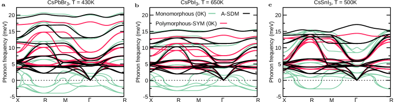
Figure 7: Phonon dispersions of cubic CsPbBr₃ at 430 K (a), CsPbI₃ at 650 K (b), and CsSnI₃ at 500 K (c) calculated using the A-SDM; all represented by black lines. Green and red lines represent the harmonic phonon dispersions of the monomorphous and polymorphous networks at 0 K. All calculations refer to 2$\times$2$\times$2 supercells and include corrections due to long-range dipole-dipole interactions.

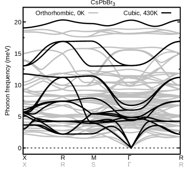
Figure 8: Phonon dispersions of cubic (430 K) and orthorhombic (0 K) CsPbBr₃ calculated using the A-SDM and FPM, respectively.

As an intermediate step to account for lattice anharmonicity, we compute temperature-dependent phonon dispersions of polymorphous cubic SrTiO₃ in the quasiharmonic approximation (QHA); i.e. we repeat phonon calculations for the polymorphous network by varying its volume according to the measured thermal lattice expansion [57]. Figure 5(a) shows the QHA phonon dispersions at 0 K, 300 K, and 500 K. The dispersions match closely each other showing that thermal lattice expansion induces small phonon frequency renormalizations. In the inset, we focus on the effect of thermal lattice expansion on the zone-center TO modes, with TO1 representing the FE soft mode. In Fig. 5(b) we present the variation of the TO1 and TO2 soft modes (diamonds) as a function of temperature calculated within the QHA. Our values are compared with theoretical data reported in Refs. [26] and  [56]. Experimental data are from Refs. [51] and [53]. Theoretical data correspond to calculations performed by combining the SCP theory with truncated Taylor expansions of the PES (SCP-TE) [14, 26] (solid lines), using the temperature-dependent effective potential (TDEP) [23] approach (filled discs) that relies on aiMD simulations, and using the stochastic self-consistent harmonic approximation (SSCHA) [22] (squares) that depends on nonperturbative supercell calculations. It is evident that the QHA combined with phonons of the polymorphous structure fails to explain data obtained with higher-level approaches to anharmonicity and experiment.

Figure 5(c) shows the temperature-dependent (anharmonic) phonon dispersions of cubic SrTiO₃ at 0 K, 300 K, 500 K, and 900 K calculated within the A-SDM. We account for thermal lattice expansion as in the QHA. In the inset, we focus on the effect of anharmonicity on the TO1 and TO2 modes. The soft nature of these modes is evidenced by their frequency sensitivity to temperature, with TO1 decreasing from 20.07 meV at 900 K to 16.58 meV at 300 K and with TO2 decreasing from 28.10 meV at 900 K to 23.75 meV at 300 K. Notably, at $T=0$ K, the AFD mode becomes unstable in the cubic phase for a 2$\times$2$\times$2 supercell even when anharmonicity is accounted for. Instead, using the tetragonal structure and including anharmonicity via the A-SDM yields stabilized phonon dispersions at $T=0$ K [black line in Fig. 5(d)] and $T=75$ K (not shown).

To make contact with existing approaches to lattice anharmonicity, in Fig. 5(e) we compare our calculations for the temperature dependence of the TO1 and TO2 phonon frequencies at the $\Gamma$-point (blue diamonds) with data reported in Refs. [26] and  [56]. Our A-SDM values in the temperature range 0–1000 K are consistent with SCP-TE, aiMD, and SSCHA data, validating the treatment of lattice anharmonicity within our methodology which includes nonperturbatively all anharmonic even-order contributions to the phonon self-energy [58]. In particular, our calculations for the TO2 phonon frequency as a function of temperature are in excellent agreement with the SCP-TE technique. In the latter approach, the phonon frequency shifts (i.e. the real part of the phonon self-energy) are evaluated through the loop diagram (four-phonon scattering) only, neglecting contributions arising from the bubble (three-phonon scattering) or higher-order diagrams. The bubble diagram is presumed to reduce the frequency renormalization of the TO1 mode [26], and is not captured in the SCP theory, and hence in the A-SDM, by construction. Upgrading A-SDM and accounting for the dynamic bubble self-energy requires the explicit evaluation of third-order force constants [59], but it is beyond the scope of this manuscript. Furthermore, it is evident that our A-SDM theory captures anharmonicity in the phonon polarization vectors through off-diagonal self-energy components since crossing between the TO1 and TO2 frequencies is avoided [26]. Small discrepancies between A-SDM and TDEP phonon frequencies of the order of 1 meV are attributed to the following possible reasons: (i) the TDEP calculations of Ref. [26] neglect thermal expansion of the crystal, (ii) TDEP accounts for the relaxation of internal coordinates along the aiMD trajectories which affects the IFCs, (iii) aiMD simulations generate a non-symmetric distribution of nuclei displacements and hence odd-order terms in the PES are accounted for, and (iv) quantum nuclear effects are absent in the TDEP approach as it relies on aiMD.

To directly compare the A-SDM with the SSCHA data of Ref. [56], we evaluate the TO1 anharmonic frequency using the tetragonal structure at $T=0$ K and $75$ K, as shown by the green diamonds in Fig. 5(e). This practically demonstrates the agreement of the two approaches for two different structural phases. Deviations between the two data sets can be explained by the fact that calculations of Ref. [56] are for $4\times 4\times 4$ supercells and include corrections from the, so called, static bubble diagram [22].

Figure 5(e) also shows that the TO1 and TO2 phonon frequencies obtained for the polymorphous cubic structure (red diamonds) are in excellent agreement with those calculated using the SCP-TE, A-SDM, and SSCHA approaches at 0 K. This result together with the phonon dispersions shown in Figs. 5(c) and (d) demonstrate that the polymorphous networks constitute a reasonable approximation for dealing with phonon anharmonicity in SrTiO₃ at low temperatures.

The temperature dependence of the TO1 phonon frequency calculated with various methods within the PBEsol approximation fails to interpret experimental data from Refs. [51] and [53], as shown in Fig. 5(e). It should be noted that the drop in the frequency observed in the TDEP data is a result of the method’s deficiency in describing quantum nuclear effects, and any improvement with respect to experimental results is merely coincidental. In reality, the TO1 phonon frequency undergoes a complex frequency shift around the phase transition temperature ($\sim 105$ K). This behavior can be described by evaluating second derivatives of the SCP free energy [21] and accounting for thermal relaxation of the internal nuclei coordinates in a quantum mechanical fashion [16]. However, the key factor that alleviates discrepancy between theory and experiment is the use of higher accuracy exchange-correlation functionals [60]. In fact, using the random-phase approximation for the treatment of electron correlation effects yields TO1 frequencies in excellent quantitative agreement with experiment [56].

In Fig. 6, we also report the variation of the AFD soft mode frequency at the R-point with temperature, yielding excellent agreement with SCP-TE data obtained for a 2$\times$2$\times$2 supercell of cubic SrTiO₃. Employing the tetragonal structure for temperatures below the phase transition, the AFD mode at $\Gamma$ splits into a double degenerate $E_{g}$ mode and an $A_{1g}$ mode. Using the experimental lattice constants [61], we found the frequency of the $E_{g}$/$A_{1g}$ mode to be 3.61/10.71 meV at $T=0$ K and 5.51/10.48 meV at $T=75$ K in agreement within 1 meV with those reported in Ref. [56]. These results further validate our A-SDM approach. We remark that the frequency of the AFD mode is expected to reduce upon increasing the supercell size [26, 18] or changing the exchange-correlation functional [56].

III.3 Metal halide perovskites: CsPbBr₃, CsPbI₃, and CsSnI₃

In Figs. 7(a)-(c), we present the phonon dispersions (black lines) of cubic CsPbBr₃, CsPbI₃, and CsSnI₃ calculated using the A-SDM for 2$\times$2$\times$2 supercells. We note that the A-SDM performance for CsPbI₃ and CsSnI₃ exhibits a similar convergence rate with the one illustrated for CsPbBr₃ (Fig. 3). We choose temperatures for which the systems remain thermodynamically stable at their cubic phases [62, 63, 64]. For comparison purposes we also include the phonons of the monomorphous (green lines) and polymorphous (red lines) structures. Our results show that IFCs of the monomorphous structures yield dynamically unstable phonons represented by the negative frequencies in the phonon dispersions (green lines). We point out that the high energy modes computed with the monomorphous structures of CsPbI3 and CsPbBr3 compare well with those obtained from the A-SDM. Polymorphism in metal halide perovskites causes a narrowing of the phonon dispersion where the majority of the high energy phonons decrease in energy, leading to enhanced phonon bunching. Interestingly, polymorphism induces the hardening of the low frequency soft modes represented by a nearly flat band along the entire X-R-M path. Instead, including anharmonicity via the A-SDM, we capture the soft mode behavior along the R-M path (black lines) which is consistent with previous calculations [20, 65]. Moreover, narrowing of the phonon density of states is not present in our A-SDM calculations. In Table 1 we provide frequencies of the FE and AFD soft modes at finite temperatures obtained with the A-SDM theory and compare them with previous calculations. Our values are in excellent agreement with SCP and aiMD data from Refs. [20], [65], and [66] apart from the $\omega_{\rm AFD}(T)$ frequency of CsPbBr₃ (2.19 meV compared to 0.95 meV). We tentatively ascribe this difference to the sensitivity of the soft mode to the choice of numerical settings, like the pseudopotential and kinetic energy cutoff and to the fact that, unlike aiMD simulations, our scheme does not allow for thermal disorder via the relaxation of nuclei coordinates. As explained in Ref. [65], phonon frequencies along the R-M path are very sensitive to variations of the interatomic forces acting between Br atoms, and thereby, to changes in the internal nuclei coordinates.

In Fig. 8 we compare the A-SDM phonon dispersion of cubic CsPbBr₃ at 430 K (black) with the harmonic one evaluated for orthorhombic CsPbBr₃ at 0 K (grey). It can be clearly seen that the two dispersions have distinct qualitative and quantitative differences, showing that phonons calculated for the orthorhombic structures do not provide a good approximation for describing anharmonicity in metal halide perovskites. For example, using the orthorhombic structure to investigate electron-phonon properties, like carrier mobilities or relaxation rates, of high-temperature phases would be inaccurate.

Table 1: Temperature-dependent frequencies of the FE soft mode at the $\Gamma$-point ($\omega_{\rm FE}$) and AFD soft mode at the R-point ($\omega_{\rm AFD}$) of cubic SrTiO₃, CsPbBr₃, CsPbI₃, and CsSnI₃. Present calculations refer to the A-SDM theory; temperatures are indicated below each compound. In the square brackets we provide the values obtained for the polymorphous structures at 0 K. Previous works’ data for SrTiO₃, CsPbBr₃, CsPbI₃, and CsSnI₃ are from Refs. [26], [65], [66], and [20]. All data refer to 2$\times$2$\times$2 supercells except those reported in Ref. [66] which are for 4$\times$4$\times$4 supercells.

	Present work		Previous works
	$\omega_{\rm FE}(T)$	$\omega_{\rm AFD}(T)$	$\omega_{\rm FE}(T)$	$\omega_{\rm AFD}(T)$
	(meV)	(meV)	(meV)	(mev)
SrTiO3	17.32 [13.86]	8.65 [9.32]	17.86	8.56
(300 K)
CsPbBr3	4.34 [4.82]	2.19 [4.55]	4.10	0.95
(430 K)
CsPbI3	3.93 [4.17]	1.96 [3.52]	3.97	2.02
(650 K)
CsSnI3	4.32 [4.44]	2.05 [3.40]	4.26	2.30
(500 K)

Table 2: Average high-frequency dielectric constant ($\epsilon^{\infty}$), and average atomic Born effective charges ($Z^{*}_{\kappa}$) of monomorphous (M) and polymorphous (P) SrTiO₃, CsPbBr₃, CsPbI₃, and CsSnI₃. Calculations were performed using 2$\times$2$\times$2 supercells.

	$\epsilon^{\infty}$	$Z^{*}_{\kappa}$
	(e)
M-SrTiO3	6.31	Sr: 2.56, Ti: 7.32,  O: -3.29
P-SrTiO3	6.12	Sr: 2.55, Ti: 7.00,  O: -3.18
M-CsPbBr3	5.31	Cs: 1.37, Pb: 4.33, Br: -1.90
P-CsPbBr3	4.61	Cs: 1.31, Pb: 4.06, Br: -1.79
M-CsPbI3	7.12	Cs: 1.44, Pb: 5.00,  I: -2.15
P-CsPbI3	5.70	Cs: 1.33, Pb: 4.42,  I: -1.92
M-CsSnI3	340.84	Cs: 1.15, Sn: 4.48,  I: -1.88
P-CsSnI3	9.91	Cs: 1.36, Sn: 5.31,  I: -2.19

Table 2 reports the average high-frequency dielectric constants ($\epsilon^{\infty}$) and atomic Born effective charges ($Z^{*}_{\kappa}$) calculated for the monomorphous and polymorphous 2$\times$2$\times$2 supercells of all cubic compounds using DFPT [67]. The averages were performed over the diagonal elements of the dielectric constant and effective charge tensors. It is evident that the cubic polymorphs of SrTiO₃, CsPbBr₃, and CsPbI₃ yield a decrease in the absolute values of $\epsilon^{\infty}$ and $Z^{*}_{\kappa}$, with the larger renormalizations found for CsPbI₃ which features the higher degree of polymorphism [68]. It is worth noting that the monomorphous CsSnI₃ exhibits an unphysically large high-frequency dielectric constant due to its metallic-like behavior in density functional theory calculations. This leads to a negligible LO-TO splitting at the $\Gamma$-point as shown by the green dispersion in Fig. 7(c). On the contrary, accounting for the polymorphous cubic CsSnI₃ yields a band gap opening and, thus, a reasonable value for the high-frequency dielectric constant of $\epsilon^{\infty}=9.91$. This value leads to an LO-TO splitting similar to the other metal halide compounds.

III.4 Zr

In this section, we study bcc Zr as a representative example of a high temperature phase, crystallizing above 1135 K [69]. In Fig. 9(a), we present the phonon dispersion (black) of bcc Zr at 1188 K evaluated using the A-SDM for a 4$\times$4$\times$4 supercell. On the same plot we include the symmetrized harmonic phonon dispersions obtained for the monomorphous (green) and polymorphous (red) structures. Unlike the phonon spectrum of the monomorphous structure, dispersions obtained with the A-SDM or the polymorphous network do not suffer from instabilities. Interestingly, the polymorphous structure constitutes a reasonable approximation for the description of the vibrational properties of bcc Zr, yielding phonon dispersions close to those calculated using the A-SDM.

To demonstrate convergence we performed calculations using supercells of different size, from 3$\times$3$\times$3 to 5$\times$5$\times$5, as shown in Fig. 9(b). Increasing the supercell size is important, not only for the more precise sampling of the effective PES, but also for approaching the limit where the nonperturbative calculation with the ZG configuration becomes exact [40]. It can be readily seen that the phonon dispersion of bcc Zr is well-converged for a 4$\times$4$\times$4 supercell. Notably, self-consistency in the A-SDM for 3$\times$3$\times$3 and 4$\times$4$\times$4 supercells was achieved using four iterations. For the A-SDM calculation in a 5$\times$5$\times$5 supercell we used only a single ZG-configuration starting from the self-consistent phonons obtained for the 4$\times$4$\times$4 supercell (step 9 of the main procedure in Sec. III.1). This component of our approach provides a significant computational advantage over aiMD which requires starting from scratch for each supercell size.

Figure 9(c) compares our calculated phonon dispersion of bcc Zr at 1188 K for a 5$\times$5$\times$5 supercell (black) with neutron scattering experiments (circles and discs) [69, 70]. Our A-SDM dispersion is in good agreement with experimental data points across the entire $\Gamma$-H-P-$\Gamma$-N high-symmetry path. We note that our results also compare well with previous theoretical works that rely on stochastic and aiMD approaches [1, 2]. The A-SDM calculations overestimate the phonon frequency of the longitudinal mode at $\frac{3}{2}(1,1,1)$ which is responsible for a martensitic transition towards the so-called $\omega$ phase [70]. This mode is, in fact, strongly overdamped and its frequency reaches down to zero. Experimental studies [69, 70] suggest contrasting conclusions on whether this behavior arises from a superlattice (elastic) reflection or inelastic scattering. Clarifying this aspect from first-principles requires updating the A-SDM to account for the internal relaxation of nuclei coordinates under external pressure and evaluating second derivatives of the free energy [16, 21].

Figure 9: (a) Phonon dispersion (black) of bcc Zr at 1188 K calculated using the A-SDM. Harmonic phonon dispersions of the monomorphous (green) and polymorphous (red) structures at 0 K are shown for comparison. All calculations refer to 4$\times$4$\times$4 supercells. (b) Convergence of the A-SDM phonon dispersions of bcc Zr at 1188 K as a function of supercell size. Green, red, and black lines represent calculations performed using 3$\times$3$\times$3, 4$\times$4$\times$4, 5$\times$5$\times$5 supercells, respectively. (c) Comparison of the phonon dispersion of bcc Zr at 1188 K calculated using the A-SDM for a 5$\times$5$\times$5 supercell (black line) with neutron scattering measurements from Refs. [69] (discs) and [70] (circles). The vertical dashed line cuts the horizontal axis at the $\frac{3}{2}(1,1,1)$ point of the reciprocal space.

IV ADDITIONAL METHODOLOGICAL CONSIDERATIONS

IV.1 Importance of using an initial polymorphous structure and iterative mixing in the A-SDM.

The main procedure for computing temperature-dependent anharmonic phonons via the A-SDM has been described in Sec. III.1. Here we discuss some numerical issues if steps 1 and 6 are overlooked. We also demonstrate the iterative linear mixing scheme used to speed up convergence.

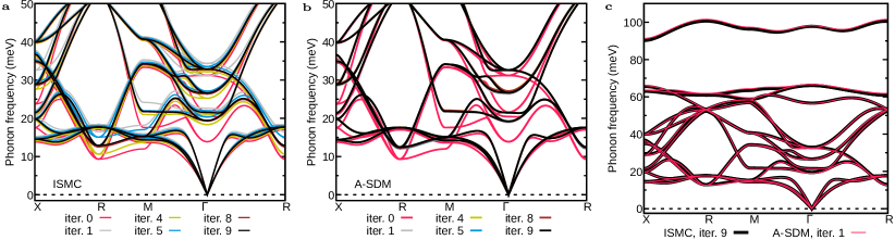
Figure 10: Iterative convergence of the phonon dispersion of cubic SrTiO₃ at 700 K calculated by (a) ISMC without mixing and (b) the A-SDM with linear mixing. In both cases, iteration 0 represents the symmetrized phonon dispersion at 0 K calculated for the polymorphous structure. (c) Self-consistent phonon dispersion of SrTiO₃ as obtained at iteration 9 by ISMC (black) and iteration 1 by the A-SDM (red). All calculations refer to 2$\times$2$\times$2 supercells.

If step 1 in the main procedure is skipped, the initial set of IFCs, $C_{p\kappa\alpha,p^{\prime}\kappa^{\prime}\alpha^{\prime}}$, might be ill-defined, resulting to imaginary phonon frequencies. This might happen if the static equilibrium positions of the nuclei do not define the global minimum of the potential [e.g. green curve in Fig. 2(b)]. Accounting for the global minimum [e.g. red curve in Fig. 2(b)] yields dynamically stable phonons. In systems with a multi-well PES featuring local saddle points, one needs to release the atoms away from their high-symmetry positions, usually defining a local maximum, and perform a tight relaxation of atomic positions (see also Sec. IV.2). This, in turn, leads to a low-symmetry distorted configuration similar to the strategy used in Ref. [42] to explore polymorphism in metal halide and oxide perovskites. We propose that the phonons calculated for the ground state polymorphous structure constitute the best starting point in the A-SDM. In general, the starting guess of the A-SDM self-consistent procedure is not necessarily unique, and one could resort to other choices (e.g. setting an electronic temperature high enough) that yield positive definite IFCs; however we consider the choice of the polymorphous structure as the most physically relevant one. Furthermore, if the harmonic approximation gives an initial positive definite IFCs matrix (see for example Ref. [71]), then the iterative procedure can start without exploring the polymorphous network.

Starting the iterative procedure from ${\bf C}_{0}$ computed for the polymorphous network guarantees dynamically stable phonons. However, if iterative mixing in step 7 is not followed, then ${\bf C}_{j}(T)$ might be ill-defined at later iterations, giving phonon instabilities. To deal with this problem one can set the imaginary frequencies to real and prepare the configuration for the next iteration, as usually performed in stochastic implementations of the SCP theory [18]. However, this practise might deteriorate the stability of the whole approach. Another issue is that the solution of ${\bf C}_{j}(T)$ might exhibit an oscillatory behavior, slowing down, or even degrading, self-consistency. In this case one can perform mixing of the oscillatory solutions of ${\bf C}_{j}(T)$ and ${\bf C}_{j-1}(T)$ and continue the iterative procedure. We encountered this issue in our preliminary tests using the Monte Carlo approach discussed below.

The oscillatory behavior and unstable solutions can be avoided, a priori, if we employ an iterative mixing of the IFCs (step 7 of the main procedure). Importantly, this approach is very beneficial for reducing statistical errors as well as for accelerating the convergence rate considerably. To demonstrate this point, in Fig. 10 we compare the convergence performances of the importance sampling Monte Carlo (ISMC) [48] approach without considering mixing with the A-SDM using linear mixing for $\beta=0.5$. We take as an example the phonon dispersion of SrTiO₃ at $T=700$ K. The ISMC framework refers to obtaining convergence of the IFCs with (i) the number of thermal configurations generated stochastically at each iteration [Eq. (II.2)] and (ii) the number of iterations. We found that 9 iterations (10 configurations each) are enough for obtaining convergence, as shown in Fig. 10(a). This amounts to a total of 90 calculations. We note that in iterations 4 and 5 of ISMC the system was trapped between two oscillatory solutions. In order to proceed to the next iteration we performed mixing of the corresponding IFCs. The A-SDM framework refers to using only one ZG configuration at each iteration which is generated by IFCs obtained through step 7 of the main procedure. The convergence performance of the A-SDM is shown in Fig. 10(b). Apart from requiring a single configuration at each iteration, the A-SDM outperforms ISMC to the point that only a signle iteration is enough for self-consistency. Figure 10(c) shows that the A-SDM and ISMC give almost identical dispersions (and free energies) at their 1^st and 9^th iterations, respectively.

Let us note that linear mixing is the simplest approach possible to introduce mixing between IFCs of different iterations. Its success for the systems studied here is remarkable, enabling convergence, essentially, with two sets of calculations. However, for more challenging or complex cases, other sophisticated schemes based on quasi-Newton methods, like the Broyden or Broyden–Fletcher–Goldfarb–Shanno (BFGS) algorithms [72, 73], could be proved useful.

IV.2 Computational details

All electronic structure calculations were performed within density functional theory (DFT) using plane waves basis sets as implemented in Quantum Espresso (QE) [74, 75]. We employed the Perdew-Burke-Ernzerhof exchange-correlation functional revised for solids (PBEsol) [76] and optimized norm-conserving Vanderbilt pseudopotentials from the PseudoDojo library [77, 78]. For cubic SrTiO₃, CsPbBr₃, CsPbI₃, and CsSnI₃ (space group $Pm\bar{3}m$) we set the kinetic energy cutoff to 120 Ry and sampled the Brillouin zone of the unit cells (5 atoms) and 2$\times$2$\times$2 supercells with 6$\times$6$\times$6 and 3$\times$3$\times$3 uniform ${\bf k}$-grids. The calculations for the tetragonal phase of SrTiO₃ (space group $I4/mcm$) were performed with the same cutoff using 4$\times$4$\times$4 and 2$\times$2$\times$2 uniform ${\bf k}$-grids for the unit cell (10 atoms) and 2$\times$2$\times$2 supercells, respectively. For bcc Zr (space group $Im\bar{3}m$) we used a cutoff of 80 Ry and sampled the Brillouin zone of the unit cell, 3$\times$3$\times$3, 4$\times$4$\times$4, and 5$\times$5$\times$5 supercells with 10$\times$10$\times$10, 4$\times$4$\times$4, 3$\times$3$\times$3, and 2$\times$2$\times$2 uniform ${\bf k}$-grids. The calculations of the high-symmetry (monomorphous) structures were performed using the unit cells with the nuclei clamped at their Wyckoff positions. The relaxed lattice constants of cubic SrTiO₃, CsPbBr₃, CsPbI₃, CsSnI₃, and Zr are found to be 3.889, 5.874, 6.251, 6.141, and 3.517 Å, respectively; for tetragonal SrTiO₃ our calculations yield $a=5.485$ and $b=7.806$ Å. These parameters were used for all calculations, unless specified otherwise. For the orthorhombic CsPbBr₃ (space group $Pnma$), we employed the unit cell containing 20 atoms and a 3$\times$3$\times$3 uniform ${\bf k}$-grid to find relaxed lattice constants of $a=7.971$, $b=8.397$, and $c=11.640$ Å. The phonons were computed using a 2$\times$2$\times$2 supercell and a 2$\times$2$\times$2 uniform ${\bf k}$-grid.

To obtain DFT ground state geometries of the cubic and tetragonal phases (the polymorphous networks), we started from the monomorphous network and displaced the nuclei away from their Wyckoff positions using ZG displacements [Eq. (12)] at $T=0$ K and the harmonic phonons. Then, we allowed the system to relax until the residual force component per atom was less than 3$\times$10^-4 eV/Å. We found that displacing the atoms along the soft modes only by switching their phonon frequencies to the real axis is a much more efficient strategy to obtain the polymorphous geometry. We made this choice because (i) ZG displacements generated for the monomorphous structure are otherwise not defined for the soft modes and (ii) the system is brought closer to its ground state. We stress that we tested various initial sets of displacements (random nudges and ZG displacements by changing signs or temperatures) that led to different polymorphous networks; however, all yield the same ground state energy and phonons [68].

The IFCs of the monomorphous and polymorphous supercell configurations were evaluated using the FPM [11, 79]. The phonon eigenmodes and eigenfrequencies at each ${\bf q}$-point were obtained by means of Fourier interpolation of the corresponding dynamical matrices. Corrections on the phonon dispersion due to long-range dipole-dipole interactions were included via the linear response approach described in Ref. [45]. High frequency dielectric constants and atomic Born effective charges were calculated using DFPT [10] as implemented in QE. ZG displacements in 2$\times$2$\times$2 supercells were employed for calculating temperature-dependent anharmonic phonons. These displacements were generated via SDM [40, 41] as implemented in the EPW/ZG code [39]. For their construction we (i) used the phonons of a zone-centered ${\bf q}$-grid commensurate with the desired supercell size, (ii) took into account dipole-dipole interaction corrections, and (iii) apply a Berry connection between the eigenmodes.

The ZG.x code implementing the A-SDM procedure with the FPM is available at the EPW/ZG module [80]. A-SDM phonon dispersions were obtained using 2$\times$2$\times$2 supercells for the perovskite structures and 3$\times$3$\times$3/4$\times$4$\times$4/5$\times$5$\times$5 supercells for bcc Zr. At each iteration, including iteration 0 for the polymorphous structure, we enforced the crystal’s symmetry operations on the IFCs. Setting the mixing parameter $\beta$ to 0.5, we found that a couple of iterations is enough to obtain reasonable convergence and a maximum of 3-4 iterations to achieve full convergence. To ensure high accuracy for the temperature dependence of the TO1 and TO2 modes of SrTiO₃, shown in Fig. 5(e), we employed 10 iterations as default. Long-range corrections in A-SDM phonon dispersions and ZG displacements were accounted for using the Born effective charges and dielectric constants of the polymorphous structures (see Table 2).

V Conclusions and outlook

In this paper, we have developed the A-SDM for the efficient treatment of anharmonicity. Similarly to previous nonperturbative methodologies, the A-SDM is based on the self-consistent phonon theory. The key feature introduced here is that special displacements can completely replace the cumbersome stochastic sampling of thermally displaced configurations, showing that a single ZG configuration is sufficient to compute temperature-dependent phonon dispersions at each iteration. Furthermore, we have demonstrated that the stability and efficiency of the self-consistent phonon approach can be considerably improved by means of an iterative linear mixing scheme. Another essential ingredient for accelerating convergence in the A-SDM is the initialization of the iterative procedure with interatomic force constants calculated for the polymorphous ground state network. Considered all together, we are suggesting, essentially, that only a couple of ZG configurations are needed to describe anharmonicity; one to obtain the polymorphous structure and one to obtain the phonon dispersion at a given temperature.

We have benchmarked our methodology for the perovskites SrTiO₃, CsPbBr₃, CsPbI₃, and CsSnI₃, which exhibit strongly anharmonic multi-well potential energy surfaces. From the calculated phonon dispersions, we have extracted temperature-dependent frequencies of soft modes at high-symmetry points and obtain excellent agreement with previous first-principles studies. We have also evaluated the phonon dispersion of the high temperature bcc phase of Zr, yielding good agreement with experiments and previous calculations. Our findings suggest that the phonons calculated for polymorphous SrTiO₃ and Zr at 0 K provide a good approximation to explore anharmonicity in these systems. We emphasize that evaluating the phonons of polymorphous networks relies on standard techniques that are routinely used for harmonic systems.

This work is also considered as the upgrade of SDM to anharmonic materials. SDM has been originally developed to automatically incorporate the effect of electron-phonon coupling in supercell calculations of band structures and optical spectra [40], and extended to other properties like transport coefficients [81]. The present study address the constraint of the harmonic approximation and opens the way for a unified treatment to electron-phonon coupling and anharmonicity in systems exhibiting a complex PES. In fact, here, we have demonstrated that the A-SDM is very effective for computing well-defined phonon dispersions of technologically important materials like the metal halide perovskites CsPbBr₃, CsPbI₃, and CsSnI₃. Anharmonicity is ubiquitous in this class of materials [82, 83, 84, 85] and interfacing efficient computations of phonons and electron-phonon couplings can shed light on their unexplored equilibrium or nonequilibrium properties [86]. Furthermore, we stress that the feature of computing thermodynamically stable phonon spectra via the A-SDM can be straightforwardly exploited by state-of-the-art perturbative electron-phonon calculations [39].

Finally, it should be possible to extend the A-SDM for the computation of phonon transport properties dominated by phonon–phonon interactions. For example, calculations of phonon relaxation times and thermal conductivity via the Green-Kubo approach should be within reach [87]. Furthermore, we expect the A-SDM to find applications in the investigation of ultrafast electron and phonon dynamics obtained by the solution of the coupled time-dependent Boltzmann equations [88, 89]. Given the generality and efficiency of our methodology, we also expect to be perfectly suited for high-throughput calculations of several electron-phonon and anharmonic properties of materials at finite temperatures.

Calculations that lead to the results of this study are available on the NOMAD repository [90].

Appendix A Proof of Eq. (7)

In this Appendix we derive Eq. (7) following the work in Ref. [21].

The expression in Eq. (II.2) is considered as the trial free energy which, according to the Gibbs-Bogolyubov inequality, provides an upper limit of the system’s free energy. Hence, the derivation of Eq. (7) relies on the minimization of the free energy with respect to the matrix of IFCs and, thus, finding the solution:

$$\frac{\partial F(T)}{\partial{C}_{\kappa\alpha,\kappa^{\prime}\alpha^{\prime}}}=0,$$ (17)

where for the sake of notation clarity we use a $\Gamma$-point formalism and drop the unit cell index $p$.

We consider first the derivative of $\braket{U}_{T}$ and use the chain rule with respect to $\tau_{\kappa\alpha}$ to obtain:

$$\frac{\partial\braket{{U}}_{T}}{\partial C_{\kappa\alpha,\kappa^{\prime}\alpha^{\prime}}}=\prod_{\nu}\!\int\!\frac{dz_{\nu}}{u_{\nu}\sqrt{2\pi}}e^{-\frac{z_{\nu}^{2}}{2u^{2}_{\nu}}}\sum_{k^{\prime\prime}\alpha^{\prime\prime}}\frac{\partial U}{\partial\tau_{\kappa^{\prime\prime}\alpha^{\prime\prime}}}\frac{\partial\tau_{\kappa^{\prime\prime}\alpha^{\prime\prime}}}{\partial C_{\kappa\alpha,\kappa^{\prime}\alpha^{\prime}}},$$

where we express the thermal average in its multivariate Gaussian integral form appearing in Eq. (II.2). We employ $\tau_{\kappa\alpha}=(M_{0}/M_{\kappa})^{1/2}\sum_{\nu}e_{\kappa\alpha,\nu}z_{\nu}$, representing the normal coordinates transformation, and apply the change of variables $z_{\nu}=\tilde{z}_{\nu}u_{\nu}$ to rewrite Eq. (A) as:

$$\frac{\partial\braket{{U}}_{T}}{\partial C_{\kappa\alpha,\kappa^{\prime}\alpha^{\prime}}}=\sum_{k^{\prime\prime}\alpha^{\prime\prime}}\bigg{(}\frac{M_{0}}{M_{\kappa^{\prime\prime}}}\bigg{)}^{1/2}\sum_{\mu}\frac{\partial\big{[}e_{\kappa^{\prime\prime}\alpha^{\prime\prime},\mu}u_{\mu}\big{]}}{\partial C_{\kappa\alpha,\kappa^{\prime}\alpha^{\prime}}}\prod_{\nu\neq\mu}\!\int\!\frac{d\tilde{z}_{\nu}}{\sqrt{2\pi}}\,e^{-\frac{\tilde{z}_{\nu}^{2}}{2}}\!\int\!\frac{d\tilde{z}_{\mu}}{\sqrt{2\pi}}\,e^{-\frac{\tilde{z}_{\mu}^{2}}{2}}\tilde{z}_{\mu}\frac{\partial U}{\partial\tau_{\kappa^{\prime\prime}\alpha^{\prime\prime}}}.$$ (19)

We perform integration by parts with respect to $\tilde{z}_{\mu}$, take the limit $\lim_{\rightarrow\infty}e^{-z^{2}}=0$, and use $\partial/\partial\tilde{z}_{\mu}=\sum_{\kappa\alpha}(M_{0}/M_{\kappa})^{1/2}e_{\kappa\alpha,\mu}u_{\mu}\,\partial/\partial\tau_{\kappa\alpha}$ to obtain the following result after some straightforward algebra:

$$\frac{\partial\braket{{U}}_{T}}{\partial C_{\kappa\alpha,\kappa^{\prime}\alpha^{\prime}}} = \frac{1}{2}\sum_{\begin{subarray}{c}\kappa^{\prime\prime}\alpha^{\prime\prime}\\ \kappa^{\prime\prime\prime}\alpha^{\prime\prime\prime}\end{subarray}}\frac{M_{0}}{\sqrt{M_{\kappa^{\prime\prime}}M_{\kappa^{\prime\prime\prime}}}}\sum_{\mu}\frac{\partial\big{[}e_{\kappa^{\prime\prime}\alpha^{\prime\prime},\mu}e_{\kappa^{\prime\prime\prime}\alpha^{\prime\prime\prime},\mu}\,u^{2}_{\mu}\big{]}}{\partial C_{\kappa\alpha,\kappa^{\prime}\alpha^{\prime}}}\Braket{\frac{\partial U}{\partial\tau_{\kappa^{\prime\prime}\alpha^{\prime\prime}}\partial\tau_{\kappa^{\prime\prime\prime}\alpha^{\prime\prime\prime}}}}_{T}.$$ (20)

Now we consider the derivative of the harmonic vibrational free energy $F_{\rm vib}(T)$ [term appearing in the second line of Eq. (II.2)] which we rewrite here for convenience:

$$F_{\rm vib}(T)=\sum_{\nu}\bigg{[}\frac{\hbar\omega_{\nu}}{2}-k_{\rm B}T\,{\rm ln}(1+n_{\nu})\bigg{]}.$$ (21)

Employing the chain rule with respect to $\omega^{2}_{\mu}$ gives:

$$\frac{\partial{F_{\rm vib}(T)}}{\partial C_{\kappa\alpha,\kappa^{\prime}\alpha^{\prime}}} = \sum_{\mu}\frac{M_{0}}{2}u^{2}_{\mu}\frac{\partial\omega^{2}_{\mu}}{\partial C_{\kappa\alpha,\kappa^{\prime}\alpha^{\prime}}},$$ (22)

where we have used $\partial n_{\nu}/\partial\omega_{\nu}^{2}=-\hbar/(2k_{\rm B}T\omega_{\nu})\,n_{\nu}(n_{\nu}+1)$. By combining Eqs. (2) and (6), and using the orthonormality relations of the phonon eigenvectors [30] we have:

$$\omega^{2}_{\mu}=\sum_{\kappa\alpha,\kappa^{\prime}\alpha^{\prime}}\frac{C_{\kappa\alpha,\kappa^{\prime}\alpha^{\prime}}}{\sqrt{M_{\kappa}M_{\kappa^{\prime}}}}e_{\kappa\alpha,\mu}\,e_{\kappa^{\prime}\alpha^{\prime},\mu},$$ (23)

that allows us to express Eq. (22) as:

$$\frac{\partial{F_{\rm vib}(T)}}{\partial C_{\kappa\alpha,\kappa^{\prime}\alpha^{\prime}}}=\frac{1}{2}\frac{M_{0}}{\sqrt{M_{\kappa}M_{\kappa^{\prime}}}}\sum_{\mu}e_{\kappa\alpha,\mu}\,e_{\kappa^{\prime}\alpha^{\prime},\mu}u^{2}_{\mu}.$$ (24)

Now we consider the vibrational energy of the effective harmonic Hamiltonian $U_{\rm h}(T)$ which we also rewrite here for convenience:

$$U_{\rm h}(T)=\frac{M_{0}}{2}\sum_{\mu}\omega^{2}_{\mu}u^{2}_{\mu}.$$ (25)

By combining Eqs. (25) and (23), and taking the derivative with respect to ${C}_{\kappa\alpha,\kappa^{\prime}\alpha^{\prime}}$ yields the following result:

$$\frac{\partial U_{\rm h}(T)}{\partial C_{\kappa\alpha,\kappa^{\prime}\alpha^{\prime}}} = \frac{1}{2}\frac{M_{0}}{\sqrt{M_{\kappa}M_{\kappa^{\prime}}}}\sum_{\mu}e_{\kappa\alpha,\mu}e_{\kappa^{\prime}\alpha^{\prime},\mu}u^{2}_{\mu}+\sum_{\begin{subarray}{c}\kappa^{\prime\prime}\alpha^{\prime\prime}\\ \kappa^{\prime\prime\prime}\alpha^{\prime\prime\prime}\end{subarray}}\frac{C_{\kappa^{\prime\prime}\alpha^{\prime\prime},\kappa^{\prime\prime\prime}\alpha^{\prime\prime\prime}}}{2}\frac{M_{0}}{\sqrt{M_{\kappa^{\prime\prime}}M_{\kappa^{\prime\prime\prime}}}}\sum_{\mu}\frac{\partial\big{[}e_{\kappa^{\prime\prime}\alpha^{\prime\prime},\mu}e_{\kappa^{\prime\prime\prime}\alpha^{\prime\prime\prime},\mu}u^{2}_{\mu}\big{]}}{\partial C_{\kappa\alpha,\kappa^{\prime}\alpha^{\prime}}}$$ (26)

Finally, we combine Eqs. (II.2), (25), and (21) together with the expressions in Eqs. (20), (26), and (24) to obtain:

$$\frac{\partial F(T)}{\partial{C}_{\kappa\alpha,\kappa^{\prime}\alpha^{\prime}}} = \frac{\partial\braket{U}_{T}}{\partial C_{\kappa\alpha,\kappa^{\prime}\alpha^{\prime}}}-\frac{\partial U_{\rm h}(T)}{\partial C_{\kappa\alpha,\kappa^{\prime}\alpha^{\prime}}}+\frac{\partial{F_{\rm vib}(T)}}{\partial C_{\kappa\alpha,\kappa^{\prime}\alpha^{\prime}}}$$ (27)

$$= \frac{1}{2}\sum_{\begin{subarray}{c}\kappa^{\prime\prime}\alpha^{\prime\prime}\\ \kappa^{\prime\prime\prime}\alpha^{\prime\prime\prime}\end{subarray}}\frac{M_{0}}{\sqrt{M_{\kappa^{\prime\prime}}M_{\kappa^{\prime\prime\prime}}}}\sum_{\mu}\frac{\partial\big{[}e_{\kappa^{\prime\prime}\alpha^{\prime\prime},\mu}e_{\kappa^{\prime\prime\prime}\alpha^{\prime\prime\prime},\mu}\,u^{2}_{\mu}\big{]}}{\partial C_{\kappa\alpha,\kappa^{\prime}\alpha^{\prime}}}\bigg{[}\Braket{\frac{\partial U}{\partial\tau_{\kappa^{\prime\prime}\alpha^{\prime\prime}}\partial\tau_{\kappa^{\prime\prime\prime}\alpha^{\prime\prime\prime}}}}_{T}-C_{\kappa^{\prime\prime}\alpha^{\prime\prime},\kappa^{\prime\prime\prime}\alpha^{\prime\prime\prime}}\bigg{]}.$$

Hence, in order to satisfy Eq. (17), the term inside the square brackets of Eq. (27) must be zero. This, essentially, completes the proof of Eq. (7) which requires evaluating the matrix of IFCs at each temperature in a self-consistent fashion.

References

- Souvatzis et al. [2008] P. Souvatzis, O. Eriksson, M. I. Katsnelson, and S. P. Rudin, Entropy driven stabilization of energetically unstable crystal structures explained from first principles theory, Phys. Rev. Lett. 100, 095901 (2008).
- Hellman et al. [2011] O. Hellman, I. A. Abrikosov, and S. I. Simak, Lattice dynamics of anharmonic solids from first principles, Phys. Rev. B 84, 180301 (2011).
- Garg et al. [2011] J. Garg, N. Bonini, B. Kozinsky, and N. Marzari, Role of disorder and anharmonicity in the thermal conductivity of silicon-germanium alloys: A first-principles study, Phys. Rev. Lett. 106, 045901 (2011).
- Errea et al. [2011] I. Errea, B. Rousseau, and A. Bergara, Anharmonic stabilization of the high-pressure simple cubic phase of calcium, Phys. Rev. Lett. 106, 165501 (2011).
- Errea et al. [2013] I. Errea, M. Calandra, and F. Mauri, First-principles theory of anharmonicity and the inverse isotope effect in superconducting palladium-hydride compounds, Phys. Rev. Lett. 111, 177002 (2013).
- Zhou et al. [2014] F. Zhou, W. Nielson, Y. Xia, and V. Ozoliņš, Lattice anharmonicity and thermal conductivity from compressive sensing of first-principles calculations, Phys. Rev. Lett. 113, 185501 (2014).
- Tadano et al. [2014] T. Tadano, Y. Gohda, and S. Tsuneyuki, Anharmonic force constants extracted from first-principles molecular dynamics: applications to heat transfer simulations, J. Phys.: Condens. Matter 26, 225402 (2014).
- Rossi et al. [2016] M. Rossi, P. Gasparotto, and M. Ceriotti, Anharmonic and quantum fluctuations in molecular crystals: A first-principles study of the stability of paracetamol, Phys. Rev. Lett. 117, 115702 (2016).
- Zacharias et al. [2020] M. Zacharias, M. Scheffler, and C. Carbogno, Fully anharmonic nonperturbative theory of vibronically renormalized electronic band structures, Phys. Rev. B 102 (2020).
- Baroni et al. [2001] S. Baroni, S. de Gironcoli, A. Dal Corso, and P. Giannozzi, Phonons and related crystal properties from density-functional perturbation theory, Rev. Mod. Phys. 73, 515 (2001).
- Kunc and Martin [1983] K. Kunc and R. M. Martin, in Ab initio calculation of phonon spectra, edited by J. Devreese, V. Van Doren, and P. Van Camp (Plenum, New York, 1983) p. 65.
- Born [1951] M. Born, Fest. Akad. D. Wiss. Göttingen, Math. Phys. Klasse (Springer, Berlin, 1951).
- Hooton [1955] D. Hooton, LI. a new treatment of anharmonicity in lattice thermodynamics: I, London Edinburgh Philos. Mag. J. Sci. 46, 422 (1955).
- Werthamer [1970] N. R. Werthamer, Self-consistent phonon formulation of anharmonic lattice dynamics, Phys. Rev. B 1, 572 (1970).
- Souvatzis et al. [2009] P. Souvatzis, O. Eriksson, M. Katsnelson, and S. Rudin, The self-consistent ab initio lattice dynamical method, Comput. Mater. Sci. 44, 888 (2009).
- Brown et al. [2013] S. E. Brown, I. Georgescu, and V. A. Mandelshtam, Self-consistent phonons revisited. II. a general and efficient method for computing free energies and vibrational spectra of molecules and clusters, Chem. Phys. 138, 044317 (2013).
- van Roekeghem et al. [2016] A. van Roekeghem, J. Carrete, and N. Mingo, Anomalous thermal conductivity and suppression of negative thermal expansion in , Phys. Rev. B 94, 020303 (2016).
- van Roekeghem et al. [2021] A. van Roekeghem, J. Carrete, and N. Mingo, Quantum self-consistent ab-initio lattice dynamics, Comput. Phys. Commun. 263, 107945 (2021).
- Errea et al. [2014] I. Errea, M. Calandra, and F. Mauri, Anharmonic free energies and phonon dispersions from the stochastic self-consistent harmonic approximation: Application to platinum and palladium hydrides, Phys. Rev. B 89, 064302 (2014).
- Patrick et al. [2015] C. E. Patrick, K. W. Jacobsen, and K. S. Thygesen, Anharmonic stabilization and band gap renormalization in the perovskite CsSnI3, Phys. Rev. B 92, 201205 (2015).
- Bianco et al. [2017] R. Bianco, I. Errea, L. Paulatto, M. Calandra, and F. Mauri, Second-order structural phase transitions, free energy curvature, and temperature-dependent anharmonic phonons in the self-consistent harmonic approximation: Theory and stochastic implementation, Phys. Rev. B 96, 014111 (2017).
- Monacelli et al. [2021] L. Monacelli, R. Bianco, M. Cherubini, M. Calandra, I. Errea, and F. Mauri, The stochastic self-consistent harmonic approximation: calculating vibrational properties of materials with full quantum and anharmonic effects, J. Phys.: Condens. Matter 33, 363001 (2021).
- Hellman et al. [2013] O. Hellman, P. Steneteg, I. A. Abrikosov, and S. I. Simak, Temperature dependent effective potential method for accurate free energy calculations of solids, Phys. Rev. B 87, 104111 (2013).
- Sun et al. [2014] T. Sun, D.-B. Zhang, and R. M. Wentzcovitch, Dynamic stabilization of cubic CaSiO3 perovskite at high temperatures and pressures from ab initio molecular dynamics, Phys. Rev. B 89, 094109 (2014).
- Bottin et al. [2020] F. Bottin, J. Bieder, and J. Bouchet, a-TDEP: Temperature dependent effective potential for abinit – lattice dynamic properties including anharmonicity, Comput. Phys. Commun. 254, 107301 (2020).
- Tadano and Tsuneyuki [2015] T. Tadano and S. Tsuneyuki, Self-consistent phonon calculations of lattice dynamical properties in cubic SrTiO3 with first-principles anharmonic force constants, Phys. Rev. B 92, 054301 (2015).
- Erba et al. [2019] A. Erba, J. Maul, M. Ferrabone, P. Carbonnière, M. Rérat, and R. Dovesi, Anharmonic vibrational states of solids from DFT calculations. part i: Description of the potential energy surface, J. Chem. Theory Comput. 15, 3755 (2019).
- Zhao et al. [2021] Y. Zhao, S. Zeng, G. Li, C. Lian, Z. Dai, S. Meng, and J. Ni, Lattice thermal conductivity including phonon frequency shifts and scattering rates induced by quartic anharmonicity in cubic oxide and fluoride perovskites, Phys. Rev. B 104, 224304 (2021).
- Ribeiro et al. [2018] G. A. S. Ribeiro, L. Paulatto, R. Bianco, I. Errea, F. Mauri, and M. Calandra, Strong anharmonicity in the phonon spectra of pbte and snte from first principles, Phys. Rev. B 97, 014306 (2018).
- Giustino [2017] F. Giustino, Electron-phonon interactions from first principles, Rev. Mod. Phys. 89, 015003 (2017).
- Ha et al. [2021] V.-A. Ha, G. Volonakis, H. Lee, M. Zacharias, and F. Giustino, Quasiparticle band structure and phonon-induced band gap renormalization of the lead-free halide double perovskite Cs2InAgCl6, J. Phys. Chem. C. 125, 21689 (2021).
- Yang et al. [2022] H. Yang, M. Govoni, A. Kundu, and G. Galli, Computational protocol to evaluate electron–phonon interactions within density matrix perturbation theory, J. Chem. Theory Comput. 18, 6031 (2022).
- Engel et al. [2022] M. Engel, H. Miranda, L. Chaput, A. Togo, C. Verdi, M. Marsman, and G. Kresse, Zero-point renormalization of the band gap of semiconductors and insulators using the projector augmented wave method, Phys. Rev. B 106, 094316 (2022).
- Lafuente-Bartolome et al. [2022] J. Lafuente-Bartolome, C. Lian, W. H. Sio, I. G. Gurtubay, A. Eiguren, and F. Giustino, Unified approach to polarons and phonon-induced band structure renormalization, Phys. Rev. Lett. 129, 076402 (2022).
- Wang et al. [2022] H. Wang, A. Tal, T. Bischoff, P. Gono, and A. Pasquarello, Accurate and efficient band-gap predictions for metal halide perovskites at finite temperature, npj Comput. Mater. 8 (2022).
- [36] T. Esswein and N. A. Spaldin, First-principles calculation of electron-phonon coupling in doped KTaO3, arXiv:2210.14113 .
- Poncé et al. [2016] S. Poncé, E. Margine, C. Verdi, and F. Giustino, Epw: Electron–phonon coupling, transport and superconducting properties using maximally localized wannier functions, Comput. Phys. Commun. 209, 116 (2016).
- Gonze et al. [2016] X. Gonze, F. Jollet, F. A. Araujo, D. Adams, B. Amadon, T. Applencourt, C. Audouze, J.-M. Beuken, J. Bieder, A. Bokhanchuk, et al., Recent developments in the ABINIT software package, Comput. Phys. Commun. 205, 106 (2016).
- Lee et al. [2023] H. Lee, S. Poncé, K. Bushick, S. Hajinazar, J. Lafuente-Bartolome, J. Leveillee, C. Lian, F. Macheda, H. Paudyal, et al., Electron-phonon physics from first principles using the EPW code, arXiv:2302.08085 (2023).
- Zacharias and Giustino [2016] M. Zacharias and F. Giustino, One-shot calculation of temperature-dependent optical spectra and phonon-induced band-gap renormalization, Phys. Rev. B 94, 075125 (2016).
- Zacharias and Giustino [2020] M. Zacharias and F. Giustino, Theory of the special displacement method for electronic structure calculations at finite temperature, Phys. Rev. Res. 2, 013357 (2020).
- Zhao et al. [2020] X.-G. Zhao, G. M. Dalpian, Z. Wang, and A. Zunger, Polymorphous nature of cubic halide perovskites, Phys. Rev. B 101, 155137 (2020).
- Giustino [2014] F. Giustino, Materials Modelling using Density Functional Theory: Properties and Predictions (Oxford University Press, Oxford, 2014) p. 199.
- Maradudin and Vosko [1968] A. A. Maradudin and S. H. Vosko, Symmetry properties of the normal vibrations of a crystal, Rev. Mod. Phys. 40, 1 (1968).
- Gonze and Lee [1997] X. Gonze and C. Lee, Dynamical matrices, born effective charges, dielectric permittivity tensors, and interatomic force constants from density-functional perturbation theory, Phys. Rev. B 55, 10355 (1997).
- Wang et al. [2010] Y. Wang, J. J. Wang, W. Y. Wang, Z. G. Mei, S. L. Shang, L. Q. Chen, and Z. K. Liu, A mixed-space approach to first-principles calculations of phonon frequencies for polar materials, J. Phys.: Condens. Matter. 22, 202201 (2010).
- Kapil et al. [2019] V. Kapil, E. Engel, M. Rossi, and M. Ceriotti, Assessment of approximate methods for anharmonic free energies, J. Chem. Theory Comput. 15, 5845 (2019).
- Zacharias et al. [2015] M. Zacharias, C. E. Patrick, and F. Giustino, Stochastic approach to phonon-assisted optical absorption, Phys. Rev. Lett. 115 (2015).
- Natarajan and Prakash [1971] M. Natarajan and B. Prakash, Phase transitions in ABX3 type halides, Phys. Status Solidi (a) 4, K167 (1971).
- Cowley et al. [1969] R. Cowley, W. Buyers, and G. Dolling, Relationship of normal modes of vibration of strontium titanate and its antiferroelectric phase transition at 110°k, Solid State Commun. 7, 181 (1969).
- Yamada and Shirane [1969] Y. Yamada and G. Shirane, Neutron scattering and nature of the soft optical phonon in SrTiO3, J. Phys. Soc. Japan 26, 396 (1969).
- Stirling [1972] W. G. Stirling, Neutron inelastic scattering study of the lattice dynamics of strontium titanate: harmonic models, J. Phys. C Solid State Phys. 5, 2711 (1972).
- Servoin et al. [1980] J. L. Servoin, Y. Luspin, and F. Gervais, Infrared dispersion in SrTiO3 at high temperature, Phys. Rev. B 22, 5501 (1980).
- Zhou et al. [2018] J.-J. Zhou, O. Hellman, and M. Bernardi, Electron-phonon scattering in the presence of soft modes and electron mobility in SrTiO3 perovskite from first principles, Phys. Rev. Lett. 121, 226603 (2018).
- Fumega et al. [2020] A. O. Fumega, Y. Fu, V. Pardo, and D. J. Singh, Understanding the lattice thermal conductivity of SrTiO3 from an ab initio perspective, Phys. Rev. Mater. 4, 033606 (2020).
- Verdi et al. [2023] C. Verdi, L. Ranalli, C. Franchini, and G. Kresse, Quantum paraelectricity and structural phase transitions in strontium titanate beyond density functional theory, Phys. Rev. Mater. 7, L030801 (2023).
- de Ligny and Richet [1996] D. de Ligny and P. Richet, High-temperature heat capacity and thermal expansion of SrTiO3 and SrZrO3 perovskites, Phys. Rev. B 53, 3013 (1996).
- Lazzeri et al. [2003] M. Lazzeri, M. Calandra, and F. Mauri, Phys. Rev. B 68 (2003).
- Paulatto et al. [2015] L. Paulatto, I. Errea, M. Calandra, and F. Mauri, First-principles calculations of phonon frequencies, lifetimes, and spectral functions from weak to strong anharmonicity: The example of palladium hydrides, Phys. Rev. B 91, 054304 (2015).
- Wahl et al. [2008] R. Wahl, D. Vogtenhuber, and G. Kresse, SrTiO3 and BaTiO3 revisited using the projector augmented wave method: Performance of hybrid and semilocal functionals, Phys. Rev. B 78, 104116 (2008).
- Okazaki and Kawaminami [1973] A. Okazaki and M. Kawaminami, Lattice constant of strontium titanate at low temperatures, Mater. Res. Bull. 8, 545 (1973).
- Hirotsu et al. [1974] S. Hirotsu, J. Harada, M. Iizumi, and K. Gesi, Structural phase transitions in CsPbBr3, J. Phys. Soc. Japan 37, 1393 (1974).
- Trots and Myagkota [2008] D. Trots and S. Myagkota, High-temperature structural evolution of caesium and rubidium triiodoplumbates, J. Phys. Chem. Solids 69, 2520 (2008).
- Yamada et al. [1991] K. Yamada, S. Funabiki, H. Horimoto, T. Matsui, T. Okuda, and S. Ichiba, Structural phase transitions of the polymorphs of CsSnI3 by means of rietveld analysis of the X-ray diffraction, Chem. Lett. 20, 801 (1991).
- Lanigan-Atkins et al. [2021] T. Lanigan-Atkins, X. He, M. J. Krogstad, D. M. Pajerowski, D. L. Abernathy, G. N. M. N. Xu, Z. Xu, D.-Y. Chung, M. G. Kanatzidis, S. Rosenkranz, et al., Two-dimensional overdamped fluctuations of the soft perovskite lattice in CsPbBr3, Nat. Mater. 20, 977 (2021).
- Ning et al. [2022] J. Ning, L. Zheng, W. Lei, S. Wang, J. Xi, and J. Yang, Temperature-dependence of the band gap in the all-inorganic perovskite CsPbI3 from room to high temperatures, Phys. Chem. Chem. Phys. 24, 16003 (2022).
- Baroni et al. [2010] S. Baroni, P. Giannozzi, and E. Isaev, Density-functional perturbation theory for quasi-harmonic calculations, Rev. Mineral. Geochem. 71, 39 (2010).
- Zacharias et al. [2023] M. Zacharias, G. Volonakis, F. Giustino, and J. Even, Anharmonic electron-phonon coupling in ultrasoft and locally disordered perovskites, arXiv:2302.09625 (2023).
- Stassis et al. [1978] C. Stassis, J. Zarestky, and N. Wakabayashi, Lattice dynamics of bcc zirconium, Phys. Rev. Lett. 41, 1726 (1978).
- Heiming et al. [1991] A. Heiming, W. Petry, J. Trampenau, M. Alba, C. Herzig, H. R. Schober, and G. Vogl, Phonon dispersion of the bcc phase of group-iv metals. ii. bcc zirconium, a model case of dynamical precursors of martensitic transitions, Phys. Rev. B 43, 10948 (1991).
- Lucrezi et al. [2022] R. Lucrezi, E. Kogler, S. Di Cataldo, M. Aichhorn, L. Boeri, and C. Heil, Quantum lattice dynamics and their importance in ternary superhydride clathrates, arXiv:2212.09789 (2022).
- Broyden [1965] C. G. Broyden, A class of methods for solving nonlinear simultaneous equations, Math. Comput. 19, 577 (1965).
- Fletcher [1987] R. Fletcher, Practical methods of optimization: V. 1-2, 2nd ed. (John Wiley & Sons, Chichester, England, 1987).
- Giannozzi et al. [2009] P. Giannozzi, S. Baroni, N. Bonini, M. Calandra, R. Car, C. Cavazzoni, D. Ceresoli, G. L. Chiarotti, M. Cococcioni, I. Dabo, et al., QUANTUM ESPRESSO: a modular and open-source software project for quantum simulations of materials, J. Phys.: Condens. Matter 21, 395502 (2009).
- Giannozzi et al. [2017] P. Giannozzi, O. Andreussi, T. Brumme, O. Bunau, M. B. Nardelli, M. Calandra, R. Car, C. Cavazzoni, D. Ceresoli, M. Cococcioni, et al., Advanced capabilities for materials modelling with quantum ESPRESSO, J. Phys.: Condens. Matter 29, 465901 (2017).
- Perdew et al. [2008] J. P. Perdew, A. Ruzsinszky, G. I. Csonka, O. A. Vydrov, G. E. Scuseria, L. A. Constantin, X. Zhou, and K. Burke, Restoring the density-gradient expansion for exchange in solids and surfaces, Phys. Rev. Lett. 100, 136406 (2008).
- Hamann [2013] D. R. Hamann, Optimized norm-conserving vanderbilt pseudopotentials, Phys. Rev. B 88, 085117 (2013).
- van Setten et al. [2018] M. van Setten, M. Giantomassi, E. Bousquet, M. Verstraete, D. Hamann, X. Gonze, and G.-M. Rignanese, The PseudoDojo: Training and grading a 85 element optimized norm-conserving pseudopotential table, Comput. Phys. Commun. 226, 39 (2018).
- Togo and Tanaka [2015] A. Togo and I. Tanaka, First principles phonon calculations in materials science, Scr. Mater. 108, 1 (2015).
- [80] http://gitlab.com/epw-code/q-e/tree/ZG .
- Gunst et al. [2017] T. Gunst, T. Markussen, M. L. N. Palsgaard, K. Stokbro, and M. Brandbyge, First-principles electron transport with phonon coupling: Large scale at low cost, Phys. Rev. B 96, 161404 (2017).
- Marronnier et al. [2017] A. Marronnier, H. Lee, B. Geffroy, J. Even, Y. Bonnassieux, and G. Roma, Structural instabilities related to highly anharmonic phonons in halide perovskites, J. Phys. Chem. Lett. 8, 2659 (2017).
- Marronnier et al. [2018] A. Marronnier, G. Roma, S. Boyer-Richard, L. Pedesseau, J.-M. Jancu, Y. Bonnassieux, C. Katan, C. C. Stoumpos, M. G. Kanatzidis, and J. Even, Anharmonicity and disorder in the black phases of cesium lead iodide used for stable inorganic perovskite solar cells, ACS Nano 12, 3477 (2018).
- Katan et al. [2018] C. Katan, A. D. Mohite, and J. Even, Entropy in halide perovskites, Nat. Mater. 17, 377 (2018).
- Ferreira et al. [2020] A. C. Ferreira, S. Paofai, A. Létoublon, J. Ollivier, S. Raymond, B. Hehlen, B. Rufflé, S. Cordier, C. Katan, J. Even, and P. Bourges, Direct evidence of weakly dispersed and strongly anharmonic optical phonons in hybrid perovskites, Commun. Phys. 3 (2020).
- Zhang et al. [2023] H. Zhang, W. Li, J. Essman, C. Quarti, I. Metcalf, W.-Y. Chiang, S. Sidhik, J. Hou, A. Fehr, A. Attar, et al., Ultrafast relaxation of lattice distortion in two-dimensional perovskites, Nat. Phys. 19, 545 (2023).
- Carbogno et al. [2017] C. Carbogno, R. Ramprasad, and M. Scheffler, Ab initio green-kubo approach for the thermal conductivity of solids, Phys. Rev. Lett. 118, 175901 (2017).
- Caruso [2021] F. Caruso, Nonequilibrium lattice dynamics in monolayer MoS2, J. Phys. Chem. Lett. 12, 1734 (2021).
- Britt et al. [2022] T. L. Britt, Q. Li, L. P. R. de Cotret, N. Olsen, M. Otto, S. A. Hassan, M. Zacharias, F. Caruso, X. Zhu, and B. J. Siwick, Direct view of phonon dynamics in atomically thin MoS2, Nano Lett. 22, 4718 (2022).
- [90] http://doi.org/10.17172/NOMAD/2023.05.13-1 .