Towards Heterogeneous Multi-core Accelerators Exploiting Fine-grained Scheduling of Layer-Fused Deep Neural Networks

Abstract

To keep up with the ever-growing performance demand of neural networks, specialized hardware (HW) accelerators are shifting towards multi-core and chiplet architectures. So far, these multi-accelerator systems exploit the increased parallelism by pipelining different NN layers across input batches on different cores to increase throughput. Yet, when pursuing this with non-batched layer-by-layer scheduling of latency-critical applications, this fails to fully exploit the available HW resources towards energy-efficient execution at the edge.

This work, therefore, enables fine-grained depth-first scheduling of layer-fused DNNs onto multi-core architectures through an open-source modeling framework called Stream. Stream is capable of representing a wide range of scheduling granularities and HW architectures and optimizes execution schedules towards minimal energy, minimal latency and/or minimal memory footprint for constrained edge devices. We validate against three SotA HW implementations employing layer-fused scheduling showing tight matching with measured efficiencies. Using Stream in further explorations, we demonstrate that high-level architectural decisions greatly impact hardware efficiency under the fine-grained scheduling paradigm, reducing the energy-delay product from $2.4\times$ for single-core architectures to up to $30\times$ for heterogeneous multi-core architectures compared to the traditional scheduling at layer granularity.

I Introduction

Deep neural networks (DNNs) have over the last decade tremendously improved performance in the fields of computer vision, natural language processing, signal analysis, etc. Yet, this progress comes at the cost of rapidly increasing network size (weights) and intermediate data values (activations). Meanwhile, the processing of these networks is moving more and more towards the edge, resulting in very tight energy, latency, and memory footprint requirements.

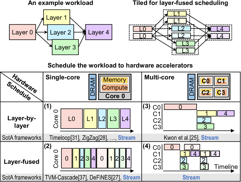
Specialized hardware (HW) architectures have co-evolved with these DNNs to accelerate their efficient inference. Traditionally, these accelerators comprise a single spatially unrolled array of processing elements (PEs), which embeds a specific dataflow [11, 5, 30, 22]. These accelerators process the DNN one layer at a time, referred to as layer-by-layer processing in Figure 1(c)(1). In order to further improve HW performance, recent architectures are shifting from a single specialized core toward multi-core designs [13, 34, 32, 21, 35, 25, 38, 12]. This increase in available computing parallelism has so far been exploited to map different DNN layers onto different cores, pipelining the execution of multiple batched inputs for increased throughput [32, 34]. However, such pipelining doesn’t provide significant benefits for latency-critical edge applications. Moreover, it results in a large memory footprint due to the coarse-grained layer-by-layer data dependencies, which are growing for modern DNNs.

To overcome the previous drawbacks, several works have investigated more fine-grained scheduling strategies of deeply fused DNN layers [2, 37, 14]. From these works, it is clear that such “layer-fused” (a.k.a. “depth-first”) scheduling can bring significant advantages for latency- and resource-constraint inference at the edge: reducing the memory footprint of intermediate results, alleviating costly off-chip accesses, and providing more parallelization opportunities. However, the SotA layer-fused schedulers work solely for their specialized HW platform and dataflows [15, 38, 26, 6]. This makes the general assessment of high-level architectural and scheduling decisions difficult. Furthermore, the fine-grained scheduling of layer-fused DNNs onto multi-core HW architectures has been largely unexplored (Figure 1(4)).

Figure 1: A conceptual example showing different ways of scheduling a deep neural network workload onto different hardware accelerators.

This work, therefore, presents the first general exploration framework of heterogeneous multi-core HW architectures with fine-grained scheduling of layer-fused DNNs. Our main contributions are:

• Stream: An open-source design space exploration framework for fine-grained scheduling of layer-fused DNNs on multi-core HW accelerators. Exploration is enabled through the combination of a unified modelling representation, a rapid fine-grained data dependency generator, a genetic algorithm-based layer-core allocator and a heuristics-based scheduler. (Section III)

• Validation of Stream with three SotA implementations of HW accelerators employing layer fusion, demonstrating accurate modelling across a wide range of scheduling granularities and HW architectures. (Section IV)

• Exploration of fine-grained scheduling of modern layer-fused DNNs onto a broad range of architectures, demonstrating up to $30\times$ EDP reduction compared to traditional layer-by-layer scheduling. (Section V)

We expect to open-source Stream soon.

II Background & Related Works

In this section, we first provide the background on DNN acceleration using specialized dataflow architectures. Next, we detail scheduling techniques of DNNs onto these architectures.

II-A Dataflow HW Architectures

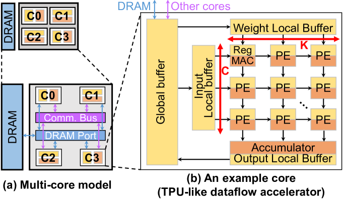
Figure 2(b) shows a traditional accelerator core architecture, constructed of an array of spatially unrolled processing elements (PEs). The array allows multiple computations to happen in parallel. In the specific architecture example in the figure, the input channels ($C$) are reused across the rows, and multiple output channels ($K$) are computed by accumulating across each column.

To increase the available compute parallelism while maintaining good utilization, the trend is to design multi-core or multi-chiplet-based architectures (Figure 2(a)). Planaria [13] devises a systolic array that can be partitioned to support an omni-directional dataflow. Illusion [32] implements an 8-chip design with minimally sized on-chip memories, connected through a sparsely-used inter-chip network. Simba [34] deploys a 36-chiplet based design, where each chiplet consists of a 4$\times$4 digital PE array. A 4$\times$4 cluster of analog in-memory compute (AiMC) cores, each housing a 1152$\times$256 capacitor-based IMC bit-cell array is prototyped in [21].

Moreover, some works shift this trend further from homogeneous to heterogeneous core combinations: a new class of heterogeneous dataflow accelerators (HDAs) that incorporate multiple sub-accelerators with varying dataflow specialization is investigated in [25]. The chip realization of DIANA [38] consists of both a digital core and an AiMC core that are interconnected through a shared on-chip memory. These heterogeneous cores provide more specialization, which can result in more efficient processing for a wider range of DNN layers.

Figure 2: (a) Multi-core architecture model. (b) Example core with specific dataflow (in red), connected to the off-chip memory port and bus for inter-core communication. All memories, ports, and the bus, have a limited bandwidth.

II-B DNN Allocation, Scheduling & Mapping

Mapping a DNN onto a multi-core HW architecture is divided into three stages:

II-B1 Layer Allocation

The recent trend towards multi-core systems enlarges the traditional mapping space. Each layer must firstly be allocated to a (set of) core(s) (from now on referred to as layer allocation). Allocating a modern DNN, which can easily consist of 50 layers, onto e.g. a quad-core architecture yields $\mathcal{O}(10^{30})$ possible layer allocations. Kwon et al. [25] explore this allocation space through a heuristics-based allocator, but does not account for the inter-core communication cost.

II-B2 Scheduling

Each allocated layer must be scheduled. This determines the execution order of the layers (or their fine-grained parts). In the traditional layer-by-layer processing, the only scheduling flexibility comes from branches in the DNN. A more fine-grained scheduling, referred to as layer-fused [2], depth-first [14] or cascaded [37] processing, and in this work referred to as layer fusion has been introduced. Instead of processing an entire layer at once, a smaller part of each layer is processed and its outputs are immediately consumed to process parts of the subsequent layers (Figure 1(2,4)). In this work, we refer to such a layer part as a computation node (CN), whose size determines the scheduling granularity. Layer fusion has two benefits compared to classical layer-by-layer scheduling: 1.) The produced and consumed activations are (depending on the layer) smaller, reducing the memory footprint, which in turn decreases the off-chip memory accesses; 2.) In a multi-core system, the computation nodes of subsequent layers can be processed in parallel if the CN data dependencies allow it, improving parallelism. However, rapidly extracting these dependencies is non-trivial for modern DNNs under fine scheduling granularity, detailed in Section III-B.

Current SotA has shown the efficacy of layer fusion for a single-core accelerator [15], homogeneous multi-cores [8, 21, 40] and heterogeneous systems [38]. However, these works only consider a limited set of DNNs with fixed scheduling granularity on specific HW architectures. TVM [37] includes a cascading scheduler that does explore different granularities and DeFiNES [27] introduces an analytical cost model enabling fast depth-first scheduling design space exploration, but they are only for single-core architectures.

II-B3 Mapping

Lastly, the computations of each CN, described by a set of for-loops, must be efficiently mapped onto each core, respecting its supported dataflow and memory resources. The dataflow plays a key role in efficiency, as a mismatch between the core’s dataflow and the CN’s computations will cause spatial under-utilization. The core’s memory hierarchy exploits the CN’s data reuse across time. Many design space exploration (DSE) frameworks have arisen [39, 24, 31, 28, 19, 18, 23], to analytically estimate the HW cost and optimize the efficiency of the mapping through loop optimizations like unrolling, tilling and reordering. However, these frameworks don’t model multi-core systems, and only estimate the HW performance of a single layer at a time.

III Stream framework

Motivation & Overview

To support the discussed trends towards multi-core DNN accelerators on the one hand, and the fine-grained scheduling on the other hand, a new high-level framework is required to rapidly co-explore various architectural and scheduling options.

To date, no framework exists that allows this co-exploration due to the difficulty in efficiently exploring the huge layer-core allocation space, rapidly extracting the fine-grained CN data dependencies, and accurately modelling the multi-core hardware communication costs. It is moreover important that the framework is easily extendable to future HW architectures, allocations and scheduling paradigms.

Therefore, this section presents a novel design space exploration framework called Stream, capable of exploring fine-grained scheduling of layer-fused DNNs onto heterogeneous multi-core architectures.

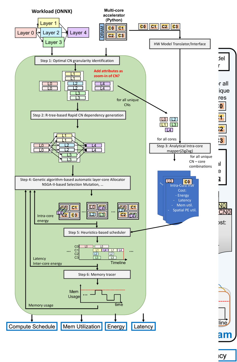
Figure 3 shows an overview of Stream: Given a DNN workload graph and a high-level multi-core accelerator architecture description, it determines an optimal compute schedule with the corresponding memory usage, energy and latency.

First, every layer is split into fine-grained computation nodes (CNs), taking into account the dataflows supported by the different accelerator cores (Step 1). Next, the data dependencies between CNs are rapidly generated and the fine-grained CN graph is formed through an R-tree [16], a tree data structure used for rapidly querying spatially separable data (Step 2). In parallel, the intra-core mapping cost of all unique CN-core combinations is optimized and extracted using a single-core DSE framework (Step 3). A genetic algorithm (GA) is subsequently deployed to explore the vast layer–core allocation space (Step 4). The GA queries a latency- and memory-prioritized scheduler that schedules the CNs onto the cores taking into account inter-core communication contention and off-chip memory access contention (Step 5).

Implementation

Figure 3: Overview of the Stream framework.

III-A CN Identification & Attribute Extraction (Step 1)

Figure 4: Computation node (CN) granularity impacts scheduling flexibility.

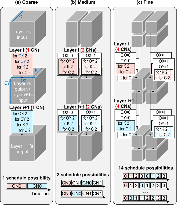
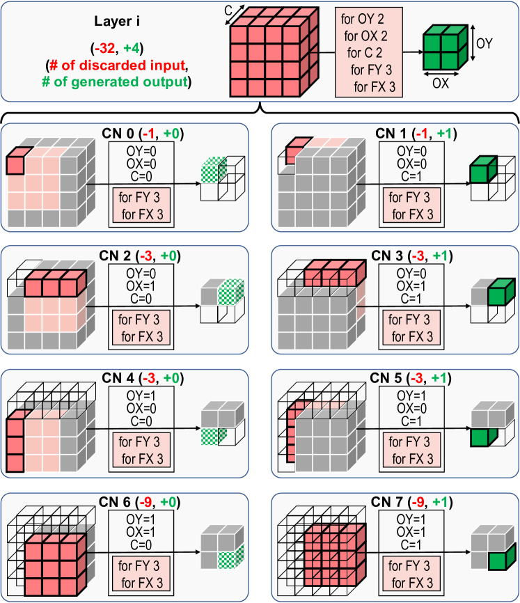
The first step of representing a layer-fused DNN is splitting each layer into multiple individually schedulable parts, referred to as computation nodes (CN). A CN is defined by isolating a subset of inner for-loops of a layer. Different subsets lead to different scheduling granularities, as shown in Figure 4. The remaining outer for-loops of a layer, called outer-CN loops, determine the CNs’ relative execution order. Stream identifies the best CN granularity using two principles:

III-A1 Layer topology awareness

The types of layers in the DNN, together with the layer interconnections impose constraints on the optimal granularity. For example, a fully connected (i.e. matrix-vector multiplication) requires all inputs to compute a single output, and the CN, therefore, contains all layer loops (i.e. the layer only contains one CN). This automatically breaks the fused layer stack. When layers do have spatial locality (e.g. convolutional layers and matrix-matrix multiplications), these loop dimensions are outer-CN loop dimensions. The outer-CN for-loops are synchronized across layers. Moreover, the out-CN loop order determines the scheduling order of CNs that belong to the same layer.

III-A2 HW dataflow awareness

When deploying a CN onto an accelerator core, the CN mapping efficiency depends on the compatibility of the spatial unrolling of the accelerator core with the dimensions of for-loops encapsulated by the CN. If the CN loop dimensions are smaller than the spatial unrolling dimensions of the targeted core, the effective HW utilization drops. To avoid such losses, the CNs are constrained to contain at least the for-loop dimensions which are spatially unrolled in the core. In the case of heterogeneous multi-core systems with multiple spatial dataflows, the CN identification constraints the CNs to minimally encompass all for-loops that are spatially unrolled in any of the cores. This ensures the minimal CN granularity with good HW utilization.

Once each layer is broken down into CNs using these principles, Stream extracts two attributes for each CN based on the ranges of the encapsulated for-loops:

1. The number of inputs exclusively used by this CN, which can hence be discarded when the CN finishes;

2. The number of final outputs newly generated by each CN, which could be sent out when the CN finishes.

Because of potential input data overlap and reduction loops across CNs, not all CNs have the same number of discardable inputs and newly generated final outputs, as shown in Figure 5. Stream’s CN attribute extraction is compatible with all layer types, strides, and padding supported by ONNX [3].

Figure 5: Computation node (CN) attribute extraction example. Attributes are the number of discarded inputs (red) and number of generated outputs (green).

III-B Fine-grained Graph Generation (Step 2)

After the identification of CNs of each layer and their attributes, the data dependencies between all CNs must be generated in order to correctly schedule the CNs in Step 5. This process is split into two parts.

Intra-layer: First, the intra-layer CN dependency edges are inserted based on the outer-CN loop order, determined in Step 1. This ensures that the required tensor accesses of CNs within a layer are structured and easily implementable using loop counters.

Inter-layer: Next, the inter-layer CN dependencies are determined based on the loop ranges of each CN. Specifically, the overlap in data generated by CNs of one layer, and required by CNs of the next layer(s), defines the data dependency between these CNs. Because this work targets a fine-grained scheduling granularity, the number of CNs could grow up to $10^{6}$ or even larger for modern DNNs. Exhaustively checking each CN pair for overlap in multi-dimensional data tensors would require $10^{12}$ checks, which is not feasible. A fast inter-layer CN dependency generator is thus required, for which an algorithm based on R-trees [16] is developed.

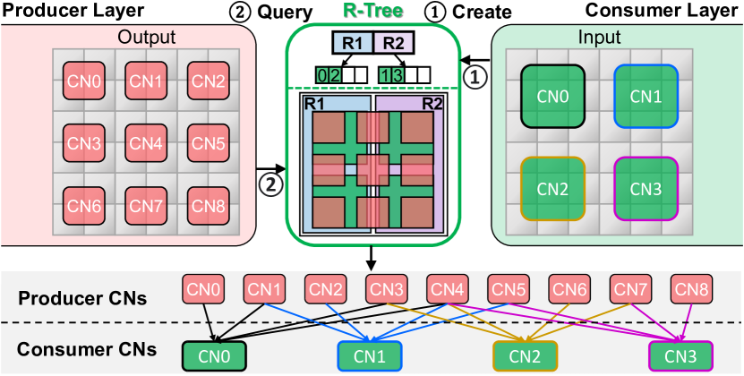
Figure 6 shows the inter-layer dependency generation for a simplified example. This process is repeated for each producer & consumer layer pair. First, an R-tree representation of all CNs of the consumer layer is created ( ), which stores the encapsulated loop ranges of each consumer CN in a tree structure. In the second step ( ), the R-tree is queried for intersection with each CN of the producer layer. The R-tree returns all consumer CNs whose ranges overlap with the range of queried producer CN. Note that in this simplified example, the 4 consumer CNs span two dimensions and are non-overlapping. In practice, they can have more dimensions with overlapping loop ranges, which is supported by Stream.

Compared with a baseline implementation of inter-layer CN dependency generation which checks every producer-consumer CN pair one-by-one, our R-tree-based algorithm is much more efficient. For a case with 448$\times$448 producer CNs and 448$\times$448 consumer CNs, the baseline implementation would take over 9 hours, whereas the R-tree-based generation takes 6 seconds ($10^{3}\times$ speedup).

III-C Intra-Core Mapping Cost Extraction (Step 3)

In this step, energy, latency, memory utilization and PE utilization of executing individual CNs on each accelerator core are extracted. As discussed earlier, multiple DSE frameworks already exist for optimizing the mapping of layer-by-layer workloads onto single-core HW architectures [39, 31, 28, 23, 19, 18]. These frameworks model the dataflow in the core and can optimize the temporal data reuse for various hardware costs such as energy, latency, EDP, etc.

In this step, the CN loops are therefore fed into such a single-core mapping optimization framework, which returns the optimal intra-core mapping and associated hardware costs. As a main objective of this work is to reduce end-to-end latency, an accurate latency estimation is crucial. We achieve this by interfacing with the ZigZag framework [28, 36], which includes an accurate latency modeling of on- and off-loading of data, as well as data stalls due to an insufficient memory bandwidth in the core [29].

The CN mapping cost extraction is modular through a HW model parser, such that other single-layer single-core DSE frameworks [39, 31, 23] can also be integrated into Stream.

Figure 6: Inter-layer CN dependency generation example using R-trees [16].

III-D Layer – Core Allocation (Step 4)

This step targets the allocation of the CNs of each layer to the different accelerator cores in the multi-core system. For large networks with varying layer types, figuring out a performant layer-core allocation can be difficult. For example, because of the fine CN granularity, it is not straightforward which CNs can execute in parallel and should hence be executed on different cores.

To this extent, a genetic algorithm (GA) is developed, as shown in Figure 3, in which the layer-core allocation is automatically optimized through the evolution of different generations of a population of layer-core allocations. We choose a GA for this allocation problem as it is modular in its optimization metrics, which can be any linear combination of latency, energy, memory footprint, or their derivatives, such as energy-delay-product (EDP). Each individual in the population receives a fitness score based on the desired metrics. The surviving individuals of a population are selected through an NSGA-II process [7], which employs advanced mechanisms to spread out the individuals over the Pareto-front. After the selection, an ordered crossover operation is performed to generate new offspring with a probability of $30\%$. Finally, the genome of an individual is randomly mutated through a bit flip (allocating a layer to a different core) or a position flip (swapping two layers’ core allocations) with a probability of $70\%$. The randomness enables the GA to escape local minima. The GA ends after a predefined number of generations, or after the desired optimization metric saturates. A Pareto front of optimal layer-core allocations is returned.

Figure 7: Step 5 - An example of fine-grained CN graph scheduling including inter-core bus communication, off-chip DRAM accesses, and memory usage trace.

III-E Multi-Core CN Scheduling (Step 5.1)

The scheduling step targets to derive the most optimal start time to execute each CN, given the fine-grained CN graph, the CN’s mapping costs and the individual’s layer-core allocation. Performing such fine-grained scheduling on a multi-core HW architecture comes with two major challenges: 1.) Correctly incorporating the inter-core communication cost stemming from the producer and consumer CNs and 2.) taking into account the cost due to off-chip fetching of the first layer(s) input activations, and of weights which do not fit in the limited on-core weight memory:

III-E1 Modeling inter-core communication

Whereas modeling the communication cost of transferring activations from core to core is relatively simple for traditional layer-by-layer execution [32], this modeling complexity grows as the computation time shrinks for finer CNs and more parallel executions appear. To model this behavior, a communication node is inserted between producer-consumer CNs mapped onto different cores. The runtime and energy cost of a communication node is calculated based on the amount of data to be transferred and the bandwidth of the data communication bus. Moreover, the bus models communication contention by scheduling all communication nodes in a first-come-first-serve manner.

III-E2 Modeling off-chip fetching

For multi-core architectures targeting edge applications, the on-chip memory resources are precious. Ideally, all weights of fused layers are stored on-chip so no off-chip weight accesses are required. However, for limited on-chip weight memory this might not be the case. Stream models both scenarios in a unified way by tracking the weights contained in each core’s on-chip memory. If a CN for which the weights are not on-chip is scheduled, the off-chip access is accounted for through the insertion of an off-chip access node for which energy and latency are modeled through an additional limited-bandwidth DRAM port. If the on-chip weight memory capacity is too small to store the new set of weights, weights are evicted from the memory in a first-in-first-out manner. At the same time, the DRAM port is used to model fetches of the input activations of the first layer.

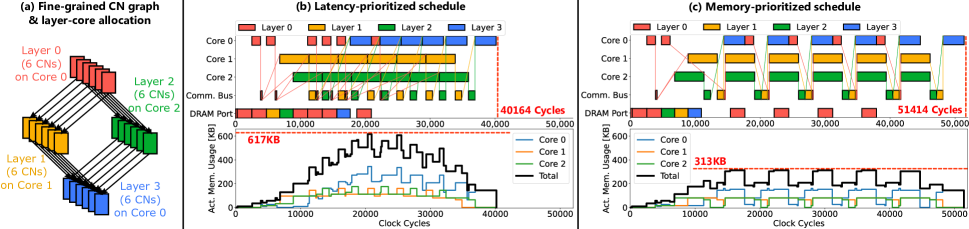
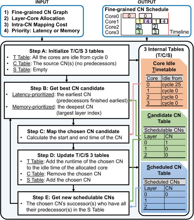
Once we have the fine-grained CN graph including the additional on-chip communication nodes and off-chip access nodes, the CNs are actually scheduled onto the cores they are allocated to. Different execution schedules will lead to different overall latencies due to the fine-grained dependencies restricting which nodes are eligible for execution. The schedule also strongly determines the memory usage: if we postpone the scheduling of a CN’s successor(s), the produced data will have to be stored in memory for a longer time. This leads to a trade-off between latency and memory footprint, as shown in Figure 7, for which Stream deploys two different scheduling optimization functions: one prioritizing minimal latency and the other prioritizing low memory usage. Their working principle is detailed in Figure 8. The scheduler keeps a pool of CN candidates, from which it selects the best candidate to schedule next based on the user-defined priority.

Latency is prioritized with the heuristic that picks the candidate whose predecessors have finished the earliest (whose data has been stored in memory the longest). This maximizes the utilization of the cores and thus benefits latency.

Memory is prioritized by picking the CN from the candidate pool that has the highest layer index. As this is the schedulable CN from the deepest layer in the fused layer stack, it stimulates the immediate consumption of data deeper into the fused stack for early discarding and efficient memory use. This can result in idle time in the core as it waits for other cores to finish the predecessors of a CN with a higher layer index, hence resulting in larger execution latency.

Figure 7 demonstrates the impact of the two prioritization strategies and the communication bus and DRAM port overhead, both in terms of latency and memory footprint of a three-core system onto which four layers are mapped. The blocks in the top of Figure 7 (b)(c) represent the CNs and the lines represent their fine-grained dependencies. The bottom figures show the memory utilization trace across time, explained next.

III-F Activation Memory Usage Tracing (Step 5.2)

Once the start and end times of all CNs are known, the activation memory utilization can be traced through time based on the number of discarded inputs and the number of generated outputs per CN (cfr. Section III-A). When a CN finishes, the inputs that are no longer required are freed from the memory space. When a CN starts, space is allocated in the memory for the to-be generated outputs. In case data is transferred between two cores, the output data of the producer CN remains in the producing core until the communication is concluded. Memory space is allocated in the consuming core as soon as the communication starts. Figure 7 shows the total memory usage trace of all three cores, of which the maximum is the peak memory usage.

Figure 8: Working principle of latency- and memory-prioritized CN Scheduler.

IV Validation

Goals. Stream is deployed to model the behavior of SotA taped-out architectures in order to demonstrate it’s modelling flexibility and quantify its modelling accuracy compared to the targets’ performance measurements.

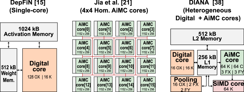
HW Targets. Figure 9 shows the three architectures considered for this validation. They are diverse in their core and memory architectures and supported scheduling granularities: 1.) DepFiN [15], a single core DNN accelerator designed for high-resolution pixel processing workloads (e.g. super-resolution, denoising) which deploys layer fusion with line-based CNs to mitigate on-chip buffer requirements; 2.) Jia et al.’s [21] multi-core architecture consisting of a 4$\times$4 array of analog in-memory-compute (AiMC) cores, enabling high throughput and energy efficiency through pipelined execution; 3.) DIANA [38], a heterogeneous multi-core AiMC + digital hybrid DNN accelerator SoC targetting efficient end-to-end inference for edge applications.

Each architecture’s specification is modelled in Stream through the: a.) intra-core characteristics for each core (operand precision, PE array size, supported dataflow, memory hierarchy) and b.) inter-core characteristics (inter-core communication protocol: bus-like or through a shared memory, inter-core constellation).

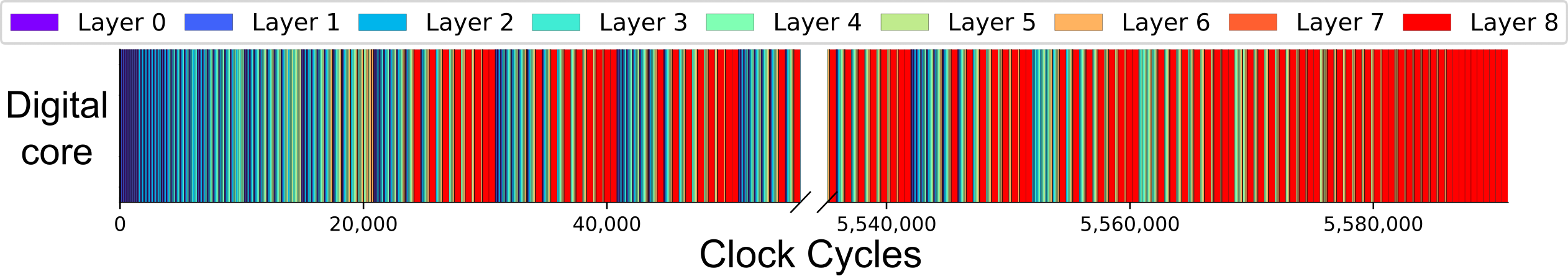
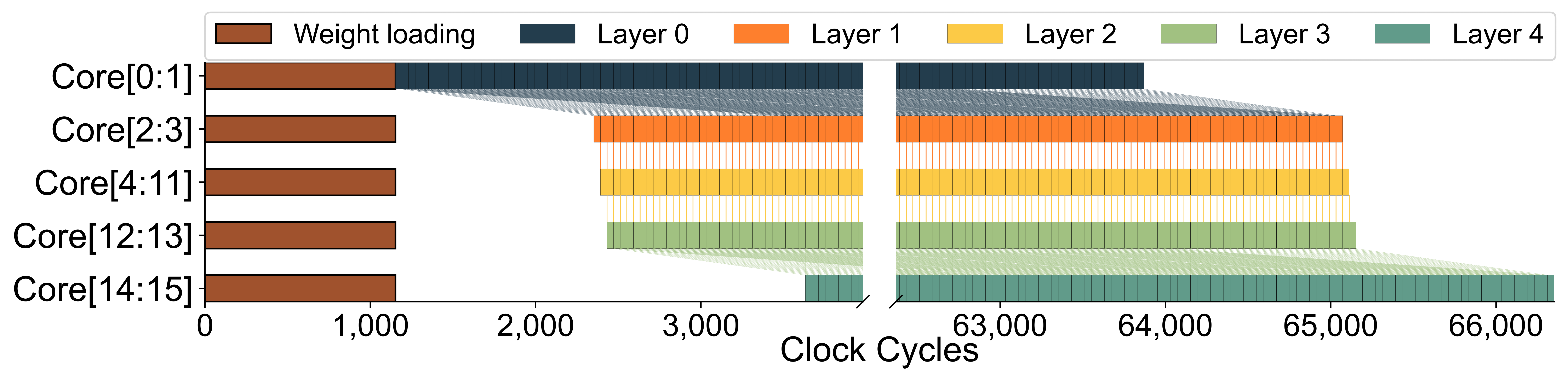
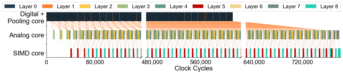
Workload Targets. Each HW target has reported the measurements of their accelerator performance for different DNNs. Each measured DNN is modelled in Stream at the scheduling granularity supported by the hardware. The mapping of the workload onto the cores is fixed and in accordance with the respective measurements, i.e. the intra-core dataflow and the core allocation used in their measurements. The latency-prioritized scheduler is applied. The validation results are summarized in Table I and the schedules generated by Stream are shown in Figure 10.

Figure 9: Hardware architecture targets for the validation of Stream.

TABLE I: Validation results for three targeted hardware architectures.

	Latency Validation
Architecture	Measured (cc)	Stream (cc)	Accuracy (%)
DepFiN [15]	$6.18\times 10^{6}$	$5.65\times 10^{6}$	91
4$\times$4 AiMC [21]	$3.66\times 10^{5}$	$3.68\times 10^{5}$	99
DIANA [38]	$8.12\times 10^{5}$	$7.83\times 10^{5}$	96
	Memory Usage Validation
Architecture	Measured (KB)	Stream (KB)	Accuracy (%)
DepFiN [15]	$238$	$244$	97
4$\times$4 AiMC [21]	N/A	$16.5$	N/A
DIANA [38]	$134$	$137$	98

IV-A DepFiN Results

The DNN used in DepFiN’s measurements is FSRCNN [9], a super-resolution CNN with large activation feature maps (560$\times$960 pixels) across the network. The large activation sizes require a peak memory usage of 28.3 MB in the traditional layer-by-layer scheduling. The modelled memory usage (244 KB) is 118$\times$ lower due to the line-buffered scheduling. Stream’s runtime was 5 seconds, and the modelled latency and memory usage are 91% , resp. 97% accurate compared to the measurement.

IV-B Multi-core AiMC Accelerator Results

The DNN model deployed by Jia et al. on their multi-core AiMC architecture are ResNet-50 segments [17]. Their work has no memory usage data available. Stream predicts a memory usage of 16.5 KB due to the tight activation balance observed in Figure 10(b). Stream’s runtime was 3 seconds, and the modelled latency is 99% accurate compared to the measurement.

IV-C DIANA Results

Lastly, we validate against DIANA’s [38] measurements of the first segment of ResNet-18 [17]. The framework is able to accurately model the fine-grained data dependencies between the varying workload operators (convolutional, pooling, element-wise sum). The different operators are mapped to the different cores, as shown in Figure 10(c). Data is shared through a 256 KB L1 memory. This would be insufficient for layer-by-layer execution, requiring frequent L2 and off-chip memory accesses. Stream’s runtime was 2 seconds, and modelled latency and memory usage are 96% , resp. 98% accurate compared to the measurement.

(a) FSRCNN on single-core DepFiN.

(b) ResNet-50 segment on 4$\times$4 AiMC multi-core.

(c) ResNet-18 segment on heterogeneous mutli-core DIANA.

Figure 10: Schedule visualization of Stream for the three validation targets.

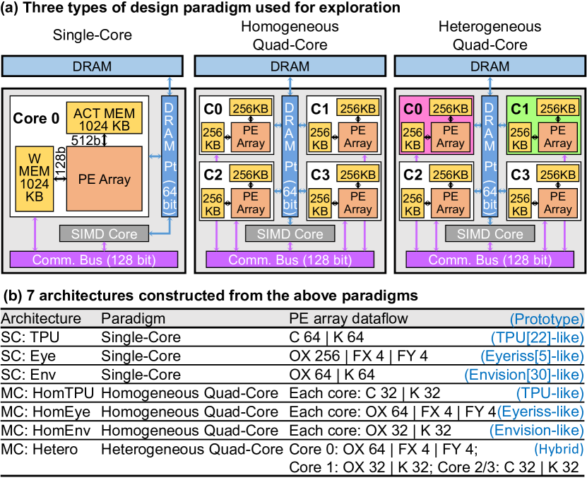
V Exploration

In this section, we deploy Stream to co-explore the optimal allocation, scheduling and mapping in combination with architectural decisions across different DNNs. For this exploration, 5 DNN workloads and 7 hardware architectures with identical area footprint are modeled. Figure 11(a) summarizes the HW configurations, in which the dataflow of each core is indicated in Figure 11(b). Each architecture houses a communication bus with a bandwidth of 128 bit/cc that is used for inter-core communication. Each core also can read/write data from/to the off-chip DRAM memory using the DRAM port, which has a shared bandwidth of 64 bit/cc. A total of 1 MB of activation and weight memory is spread across the cores and all memory read and write costs are automatically extracted through CACTI 7 [4].

V-A Automated Layer-core Allocation Impact

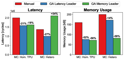
First, we explore the impact of the genetic algorithm-based automatic layer-core allocation by comparing it to a manual allocation. While for classical layer-by-layer scheduling allocation can be done manually with simple heuristics, the fine-grained scheduling space is too large for manual allocation.

We compare the automatic GA-based allocation to a manual allocation for ResNet-18 onto both a homogeneous (HomTPU in Figure 11) and a heterogeneous (Hetero in Figure 11) quad-core architecture. The manual assignment for the homogeneous architecture allocates layers to subsequent cores in a ping-pong fashion, while for the heterogeneous architectures allocation is done by assigning CNs to the core with the best fits the dataflow of that layer (best spatial utilization). The multi-core scheduler is run with both the latency priority and memory priority (cfr. Section III-E). The results in Figure 12 show that the automatic allocation provides a significant reduction in both latency and memory requirements. Moreover, the different priority schedules show the latency – memory trade-off: the GA’s memory leader has 56 % lower memory usage at a 54 % higher latency on the heterogeneous architecture. All further experiments, both for coarse and fine granularities, are executed using the GA-based allocation with the latency scheduling priority.

Figure 11: Seven hardware architectures used for architecture exploration.

V-B Architecture Impact

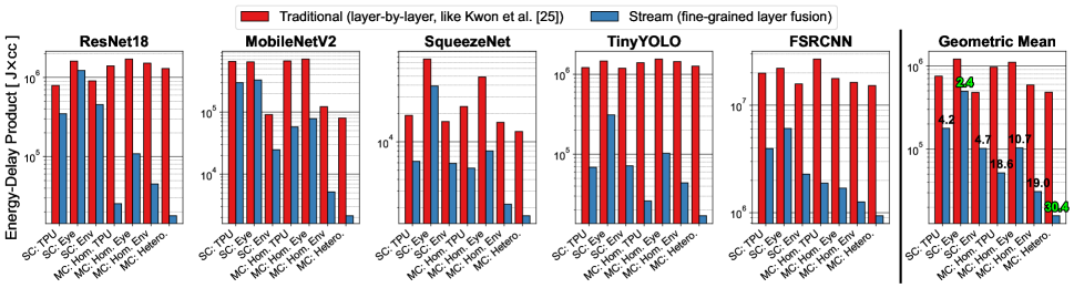
Next, we explore the capabilities of Stream to assess the benefits and drawbacks of various hardware architectures for fine-grained layer-fused DNN execution. A diverse set of neural network models is used for this study: ResNet18 [17], MobileNetV2 [33], SqueezeNet [20], Tiny-YOLO [1] and FSRCNN [10].

Stream optimally allocates each dense computational layer to one of the accelerator cores using its genetic algorithm, while the other layers such pooling and residual addition layers are assigned to the additional SIMD core. To demonstrate Stream’s optimization flexibility, this study targets energy-delay-product (EDP) as the allocation’s optimization criterion.

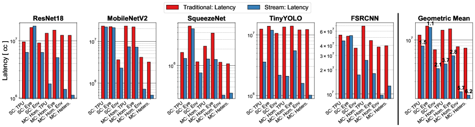
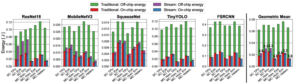
The results of all experiments are summarized in Figure 13. For each combination of workload and architecture, the EDP is optimized for both layer-by-layer scheduling granularity, as used by the SotA scheduler of Kwon et al. [25] and a fine-grained scheduling granularity. We also show the impact of the design choices on the latency and energy individually in Figures 14 & 15 respectively, for the optimal EDP point.

We break our analysis down into the three modelled architecture classes:

V-B1 Single-Core Architectures

Layer fusion consistently outperforms layer-by-layer processing. First, there are latency benefits from fusion because pooling layer CNs can be executed in the SIMD core in parallel to the convolutional layer CNs. Another reason for improved latency and energy is the reduced size of the activations, enabling on-chip storage, preventing all features to be sent to DRAM and back. This is observed in Figure 15, where the layer-fused scheduling of Stream results in lower off-chip energy compared to traditional layer-by-layer scheduling. For the three single-core architectures, the EDP gains for the geometric mean over the networks between layer-by-layer and layer fusion are between $2.4\times$ and $4.7\times$.

V-B2 Homogeneous Multi-core Architectures

The homogeneous multi-core architecture results demonstrate that multi-core is not always better than single-core, at least not under the layer-by-layer scheduling granularity. This is due to the fact that each single smaller core has a lower hardware efficiency for workloads with coarse scheduling granularity. For fine-grained layer fusion, homogeneous multi-core architectures do consistently outperform single-core architectures, as they bring more parallelization opportunities, increasing the temporal utilization (i.e. the percentage of time the core is active). Moreover, the off-chip DRAM energy is further reduced. For the three homogeneous multi-core architectures, layer fusion has between $10\times$ and $19\times$ better EDP than layer-by-layer scheduling.

Figure 12: Impact of the automatic layer-core allocation. The GA solution has significantly better latency and memory requirement than manual allocation.

Figure 13: The best EDP point found by Stream over 5 DNNs for 7 hardware architectures under traditional layer-by-layer scheduling and fine-grained layer fusion. The architecture abbreviations are shown in Figure 11(b). For the geometric mean, the EDP reduction from layer-by-layer to layer-fused is shown.

V-B3 Heterogeneous Multi-core Architecture

In the heterogeneous multi-core architecture, multiple dataflows provide specialization to serve a broader range of networks with widely varying layer topologies at higher spatial utilization, improving the latency in comparison with the best-performing homogeneous architecture. From this, it is clearly shown both layer-fused and multi-core execution improve latency. Uniform networks, like SqueezeNet or FSRCNN already experience a good matching between their layer topologies and the dataflow for the homogeneous multi-cores designs. These networks, as a result, benefit less from heterogeneous multi-core mappings or have even decreased latency performance, because the heterogeneous system includes cores with dataflows less optimal for these networks. Other networks benefit more from heterogeneity due to their variety in layer types. The wider the variety in layers, the more the benefit from the heterogeneity. Averaged across all studied networks, the explored heterogeneous architecture has an overall $1.6\times$ better EDP than the best performing homogeneous architecture, under fine-grained layer fusion. Moreover, layer fusion has $30.4\times$ better EDP than layer-by-layer execution.

Figure 14: Latency for the best EDP points of the exploration.

Figure 15: Energy breakdown for the best EDP points of the exploration.

In summary, Stream allows us to quantitatively and automatically co-explore the optimal scheduling granularity with architectural decisions, providing insight into the hardware performance of fine-grained layer fusion on a broad range of single- & multi-core architectures.

VI Conclusion

This work presented Stream, the first open-source modelling framework capable of representing layer-fused deep neural networks across a wide range of scheduling granularities and heterogeneous multi-core architectures. Stream optimizes execution schedules towards minimal energy, minimal latency and/or minimal memory footprint for constrained edge devices. The framework is validated against three state-of-the-art hardware implementations employing layer-fused scheduling, showing tight matching with measured hardware efficiencies. Moreover, we demonstrated that high-level architectural decisions greatly impact hardware efficiency under the fine-grained scheduling paradigm, reducing energy-delay-product from $2.4\times$ for single-core architectures to $30\times$ for heterogeneous multi-core architectures compared to the traditional scheduling at layer granularity.

References

- [1] P. Adarsh, P. Rathi, and M. Kumar, “YOLO v3-Tiny: Object Detection and Recognition using one stage improved model,” in 2020 6th International Conference on Advanced Computing and Communication Systems (ICACCS). IEEE, 2020, pp. 687–694.
- [2] M. Alwani, H. Chen, M. Ferdman, and P. Milder, “Fused-layer CNN accelerators,” in 2016 49th Annual IEEE/ACM International Symposium on Microarchitecture (MICRO), 2016, pp. 1–12.
- [3] J. Bai, F. Lu, K. Zhang et al., “ONNX: Open Neural Network Exchange,” https://github.com/onnx/onnx, 2019.
- [4] R. Balasubramonian, A. B. Kahng, N. Muralimanohar, A. Shafiee, and V. Srinivas, “CACTI 7: New tools for interconnect exploration in innovative off-chip memories,” ACM Transactions on Architecture and Code Optimization (TACO), vol. 14, no. 2, pp. 1–25, 2017.
- [5] Y.-H. Chen, T. Krishna, J. S. Emer, and V. Sze, “Eyeriss: An Energy-Efficient Reconfigurable Accelerator for Deep Convolutional Neural Networks,” IEEE Journal of Solid-State Circuits, vol. 52, no. 1, pp. 127–138, 2017.
- [6] S. Colleman and M. Verhelst, “High-utilization, high-flexibility depth-first CNN coprocessor for image pixel processing on FPGA,” IEEE Transactions on Very Large Scale Integration (VLSI) Systems, vol. 29, no. 3, pp. 461–471, 2021.
- [7] K. Deb, A. Pratap, S. Agarwal, and T. Meyarivan, “A fast and elitist multiobjective genetic algorithm: NSGA-II,” IEEE transactions on evolutionary computation, vol. 6, no. 2, pp. 182–197, 2002.
- [8] Y. Ding, L. Zhu, Z. Jia, G. Pekhimenko, and S. Han, “IOS: Inter-operator scheduler for cnn acceleration,” Proceedings of Machine Learning and Systems, vol. 3, pp. 167–180, 2021.
- [9] C. Dong, C. C. Loy, and X. Tang, “Accelerating the Super-Resolution Convolutional Neural Network,” CoRR, vol. abs/1608.00367, 2016. [Online]. Available: http://arxiv.org/abs/1608.00367
- [10] C. Dong, C. C. Loy, and X. Tang, “Accelerating the super-resolution convolutional neural network,” in European conference on computer vision. Springer, 2016, pp. 391–407.
- [11] Z. Du, R. Fasthuber, T. Chen, P. Ienne, L. Li, T. Luo, X. Feng, Y. Chen, and O. Temam, “ShiDianNao: Shifting vision processing closer to the sensor,” in 2015 ACM/IEEE 42nd Annual International Symposium on Computer Architecture (ISCA), 2015, pp. 92–104.
- [12] A. Garofalo, G. Ottavi, F. Conti, G. Karunaratne, I. Boybat, L. Benini, and D. Rossi, “A Heterogeneous In-Memory Computing Cluster For Flexible End-to-End Inference of Real-World Deep Neural Networks,” arXiv preprint arXiv:2201.01089, 2022.
- [13] S. Ghodrati, B. H. Ahn, J. Kyung Kim, S. Kinzer, B. R. Yatham, N. Alla, H. Sharma, M. Alian, E. Ebrahimi, N. S. Kim, C. Young, and H. Esmaeilzadeh, “Planaria: Dynamic Architecture Fission for Spatial Multi-Tenant Acceleration of Deep Neural Networks,” in 2020 53rd Annual IEEE/ACM International Symposium on Microarchitecture (MICRO), 2020, pp. 681–697.
- [14] K. Goetschalckx and M. Verhelst, “Breaking High-Resolution CNN Bandwidth Barriers With Enhanced Depth-First Execution,” IEEE Journal on Emerging and Selected Topics in Circuits and Systems, vol. 9, no. 2, pp. 323–331, 2019.
- [15] K. Goetschalckx and M. Verhelst, “DepFiN: A 12nm, 3.8TOPs depth-first CNN processor for high res. image processing,” in 2021 Symposium on VLSI Circuits, 2021, pp. 1–2.
- [16] A. Guttman, “R-Trees: A Dynamic Index Structure for Spatial Searching,” in Proceedings of the 1984 ACM SIGMOD International Conference on Management of Data, ser. SIGMOD ’84. New York, NY, USA: Association for Computing Machinery, 1984, p. 47–57. [Online]. Available: https://doi.org/10.1145/602259.602266
- [17] K. He, X. Zhang, S. Ren, and J. Sun, “Deep residual learning for image recognition,” in Proceedings of the IEEE conference on computer vision and pattern recognition, 2016, pp. 770–778.
- [18] K. Hegde, P.-A. Tsai, S. Huang, V. Chandra, A. Parashar, and C. W. Fletcher, “Mind Mappings: Enabling Efficient Algorithm-Accelerator Mapping Space Search,” in Proceedings of the 26th ACM International Conference on Architectural Support for Programming Languages and Operating Systems, ser. ASPLOS 2021. New York, NY, USA: Association for Computing Machinery, 2021, p. 943–958. [Online]. Available: https://doi.org/10.1145/3445814.3446762
- [19] Q. Huang, A. Kalaiah, M. Kang, J. Demmel, G. Dinh, J. Wawrzynek, T. Norell, and Y. S. Shao, “CoSA: Scheduling by Constrained Optimization for Spatial Accelerators,” in 2021 ACM/IEEE 48th Annual International Symposium on Computer Architecture (ISCA), 2021, pp. 554–566.
- [20] F. N. Iandola, S. Han, M. W. Moskewicz, K. Ashraf, W. J. Dally, and K. Keutzer, “SqueezeNet: AlexNet-level accuracy with 50x fewer parameters and¡ 0.5 MB model size,” arXiv preprint arXiv:1602.07360, 2016.
- [21] H. Jia, M. Ozatay, Y. Tang, H. Valavi, R. Pathak, J. Lee, and N. Verma, “Scalable and Programmable Neural Network Inference Accelerator Based on In-Memory Computing,” IEEE Journal of Solid-State Circuits, vol. 57, no. 1, pp. 198–211, 2022.
- [22] N. P. Jouppi, C. Young, N. Patil, D. Patterson, G. Agrawal, R. Bajwa, S. Bates, S. Bhatia, N. Boden, A. Borchers, R. Boyle, P.-l. Cantin, C. Chao, C. Clark, J. Coriell, M. Daley, M. Dau, J. Dean, B. Gelb, T. Vazir Ghaemmaghami, R. Gottipati, W. Gulland, R. Hagmann, C. R. Ho, D. Hogberg, J. Hu, R. Hundt, D. Hurt, J. Ibarz, A. Jaffey, A. Jaworski, A. Kaplan, H. Khaitan, A. Koch, N. Kumar, S. Lacy, J. Laudon, J. Law, D. Le, C. Leary, Z. Liu, K. Lucke, A. Lundin, G. MacKean, A. Maggiore, M. Mahony, K. Miller, R. Nagarajan, R. Narayanaswami, R. Ni, K. Nix, T. Norrie, M. Omernick, N. Penukonda, A. Phelps, J. Ross, M. Ross, A. Salek, E. Samadiani, C. Severn, G. Sizikov, M. Snelham, J. Souter, D. Steinberg, A. Swing, M. Tan, G. Thorson, B. Tian, H. Toma, E. Tuttle, V. Vasudevan, R. Walter, W. Wang, E. Wilcox, and D. H. Yoon, “In-Datacenter Performance Analysis of a Tensor Processing Unit,” arXiv e-prints, p. arXiv:1704.04760, Apr. 2017.
- [23] S.-C. Kao and T. Krishna, “GAMMA: Automating the HW Mapping of DNN Models on Accelerators via Genetic Algorithm,” in ICCAD, 2020.
- [24] H. Kwon, P. Chatarasi, V. Sarkar, T. Krishna, M. Pellauer, and A. Parashar, “MAESTRO: A Data-Centric Approach to Understand Reuse, Performance, and Hardware Cost of DNN Mappings,” IEEE Micro, vol. 40, no. 3, pp. 20–29, 2020.
- [25] H. Kwon, L. Lai, M. Pellauer, T. Krishna, Y. hsin Chen, and V. Chandra, “Heterogeneous Dataflow Accelerators for Multi-DNN Workloads,” 2021 IEEE International Symposium on High-Performance Computer Architecture (HPCA), pp. 71–83, 2021.
- [26] Z. Liu, J. Leng, Q. Chen, C. Li, W. Zheng, L. Li, and M. Guo, “DLFusion: An Auto-Tuning Compiler for Layer Fusion on Deep Neural Network Accelerator,” in 2020 IEEE Intl Conf on Parallel & Distributed Processing with Applications, Big Data & Cloud Computing, Sustainable Computing & Communications, Social Computing & Networking (ISPA/BDCloud/SocialCom/SustainCom). IEEE, 2020, pp. 118–127.
- [27] L. Mei, K. Goetschalckx, A. Symons, and M. Verhelst, “DeFiNES: Enabling Fast Exploration of the Depth-first Scheduling Space for DNN Accelerators through Analytical Modeling,” arXiv e-prints, p. arXiv:2212.05344, Dec. 2022.
- [28] L. Mei, P. Houshmand, V. Jain, S. Giraldo, and M. Verhelst, “ZigZag: Enlarging Joint Architecture-Mapping Design Space Exploration for DNN Accelerators,” IEEE Transactions on Computers, vol. 70, no. 8, pp. 1160–1174, 2021.
- [29] L. Mei, H. Liu, T. Wu, H. E. Sumbul, M. Verhelst, and E. Beigne, “A Uniform Latency Model for DNN Accelerators with Diverse Architectures and Dataflows,” in 2022 Design, Automation & Test in Europe Conference & Exhibition (DATE), 2022, pp. 220–225.
- [30] B. Moons, R. Uytterhoeven, W. Dehaene, and M. Verhelst, “14.5 Envision: A 0.26-to-10TOPS/W subword-parallel dynamic-voltage-accuracy-frequency-scalable Convolutional Neural Network processor in 28nm FDSOI,” in 2017 IEEE International Solid-State Circuits Conference, ISSCC 2017, San Francisco, CA, USA, February 5-9, 2017. IEEE, 2017, pp. 246–247. [Online]. Available: https://doi.org/10.1109/ISSCC.2017.7870353
- [31] A. Parashar, P. Raina, Y. S. Shao, Y.-H. Chen, V. A. Ying, A. Mukkara, R. Venkatesan, B. Khailany, S. W. Keckler, and J. Emer, “Timeloop: A Systematic Approach to DNN Accelerator Evaluation,” in 2019 IEEE International Symposium on Performance Analysis of Systems and Software (ISPASS), 2019, pp. 304–315.
- [32] R. Radway, A. Bartolo, P. Jolly, Z. Khan, B. Le, P. Tandon, T. Wu, Y. Xin, E. Vianello, P. Vivet, E. Nowak, H.-S. P. Wong, M. Sabry, E. Beigne, M. Wootters, and S. Mitra, “Illusion of large on-chip memory by networked computing chips for neural network inference,” Nature Electronics, vol. 4, 01 2021.
- [33] M. Sandler, A. Howard, M. Zhu, A. Zhmoginov, and L.-C. Chen, “Mobilenetv2: Inverted residuals and linear bottlenecks,” in Proceedings of the IEEE conference on computer vision and pattern recognition, 2018, pp. 4510–4520.
- [34] Y. S. Shao, J. Clemons, R. Venkatesan, B. Zimmer, M. Fojtik, N. Jiang, B. Keller, A. Klinefelter, N. Pinckney, P. Raina, S. G. Tell, Y. Zhang, W. J. Dally, J. Emer, C. T. Gray, B. Khailany, and S. W. Keckler, “Simba: Scaling Deep-Learning Inference with Multi-Chip-Module-Based Architecture,” in Proceedings of the 52nd Annual IEEE/ACM International Symposium on Microarchitecture, ser. MICRO ’52. New York, NY, USA: Association for Computing Machinery, 2019, p. 14–27. [Online]. Available: https://doi.org/10.1145/3352460.3358302
- [35] D. Shin, J. Lee, J. Lee, J. Lee, and H.-J. Yoo, “DNPU: An energy-efficient deep-learning processor with heterogeneous multi-core architecture,” IEEE Micro, vol. 38, no. 5, pp. 85–93, 2018.
- [36] A. Symons, L. Mei, and M. Verhelst, “LOMA: Fast Auto-Scheduling on DNN Accelerators through Loop-Order-based Memory Allocation,” in 2021 IEEE 3rd International Conference on Artificial Intelligence Circuits and Systems (AICAS), 2021, pp. 1–4.
- [37] tvm rfcs, “Arm® Ethos™-U Cascading Scheduler.” [Online]. Available: https://github.com/apache/tvm-rfcs/blob/main/rfcs/0037-arm-ethosu-cascading-scheduler.md
- [38] K. Ueyoshi, I. A. Papistas, P. Houshmand, G. M. Sarda, V. Jain, M. Shi, Q. Zheng, S. Giraldo, P. Vrancx, J. Doevenspeck, D. Bhattacharjee, S. Cosemans, A. Mallik, P. Debacker, D. Verkest, and M. Verhelst, “DIANA: An End-to-End Energy-Efficient Digital and ANAlog Hybrid Neural Network SoC,” in 2022 IEEE International Solid- State Circuits Conference (ISSCC), vol. 65, 2022, pp. 1–3.
- [39] X. Yang, M. Gao, Q. Liu, J. Setter, J. Pu, A. Nayak, S. Bell, K. Cao, H. Ha, P. Raina, C. Kozyrakis, and M. Horowitz, Interstellar: Using Halide’s Scheduling Language to Analyze DNN Accelerators. New York, NY, USA: Association for Computing Machinery, 2020, p. 369–383. [Online]. Available: https://doi.org/10.1145/3373376.3378514
- [40] S. Zheng, Y. Liang, S. Wang, R. Chen, and K. Sheng, FlexTensor: An Automatic Schedule Exploration and Optimization Framework for Tensor Computation on Heterogeneous System. New York, NY, USA: Association for Computing Machinery, 2020, p. 859–873. [Online]. Available: https://doi.org/10.1145/3373376.3378508