RangeAugment: Efficient Online Augmentation with Range Learning

Abstract

State-of-the-art automatic augmentation methods (e.g., AutoAugment and RandAugment) for visual recognition tasks diversify training data using a large set of augmentation operations. The range of magnitudes of many augmentation operations (e.g., brightness and contrast) is continuous. Therefore, to make search computationally tractable, these methods use fixed and manually-defined magnitude ranges for each operation, which may lead to sub-optimal policies. To answer the open question on the importance of magnitude ranges for each augmentation operation, we introduce RangeAugment that allows us to efficiently learn the range of magnitudes for individual as well as composite augmentation operations. RangeAugment uses an auxiliary loss based on image similarity as a measure to control the range of magnitudes of augmentation operations. As a result, RangeAugment has a single scalar parameter for search, image similarity, which we simply optimize via linear search. RangeAugment integrates seamlessly with any model and learns model- and task-specific augmentation policies. With extensive experiments on the ImageNet dataset across different networks, we show that RangeAugment achieves competitive performance to state-of-the-art automatic augmentation methods with 4-5 times fewer augmentation operations. Experimental results on semantic segmentation, object detection, foundation models and knowledge distillation further shows RangeAugment’s effectiveness.

Model	Aug. method	Search space	Train time overhead†	Top-1
MobileNetv2-1.0	AutoAugment	$O\left(\left(MNP\right)^{2L}\right)$	$25\%\pm 5\%$	72.7%
	RandAugment	$O(MN)$	$25\%\pm 5\%$	72.1%
	RangeAugment (Ours)	$O(1)$	$2\%\pm 1\%$	73.0%
ResNet-101	AutoAugment	$O\left(\left(MNP\right)^{2L}\right)$	$25\%\pm 5\%$	81.4%
	RandAugment	$O(MN)$	$25\%\pm 5\%$	81.5%
	RangeAugment (Ours)	$O(1)$	$2\%\pm 1\%$	81.9%

(a) ImageNet classification

Backbone	RangeAugment	mIoU
MobileNetv2-1.0	✗	38.0%
	✓	38.6%
ResNet-101	✗	45.7%
	✓	46.5%

(b) ADE20k semantic segmentation with DeepLabv3

Backbone	RangeAugment	BBox mAP	Seg. mAP
MobileNetv2-1.0	✗	37.2%	33.4%
	✓	38.4%	34.7%
ResNet-101	✗	45.6%	40.4%
	✓	46.1%	41.1%

(c) MS-COCO object detection with Mask R-CNN

Model	Dataset size	RangeAugment	0-shot Top-1
CLIP ViT-B	302 M	✗	67.1%
	302 M	✓	68.3%
CLIP ViT-H	2.0 B	✗	78.0%
	1.1 B	✓	77.9%

(d) Foundation models

Table 1: RangeAugment: Learning model- and task-specific augmentation policies online for visual recognition tasks efficiently at scale. Here, $M$, $N$, $P$, and $L$ denotes the number of magnitude bins, augmentation operations, probability bins, and augmentation policies respectively. ^†Training time overhead is computed with respect to the baseline model trained without any augmentation.

1 Introduction

Data augmentation is a widely used regularization method for training deep neural networks (LeCun et al., 1998; Krizhevsky et al., 2012; Szegedy et al., 2015; Perez & Wang, 2017; Steiner et al., 2021). These methods apply carefully designed augmentation (or image transformation) operations (e.g., color transforms) to increase the quantity and diversity of training data, which in turn helps improve the generalization ability of models. However, these methods rely heavily on expert knowledge and extensive trial-and-error experiments.

Recently, automatic augmentation methods have gained attention because of their ability to search for augmentation policy (e.g., combinations of different augmentation operations) that maximizes validation performance (Cubuk et al., 2019; 2020; Lim et al., 2019; Hataya et al., 2020; Zheng et al., 2021). In general, most augmentation operations (e.g., brightness and contrast) are parameterized by two variables: (1) the probability of applying them and (2) their range of magnitudes. These methods take a set of augmentation operations with a fixed (often discretized) range of magnitudes as an input, and produce a policy of applying some or all augmentation operations along with their parameters (Fig. 1). As an example, AutoAugment (Cubuk et al., 2019) discretizes the range of magnitudes and probabilities of 16 augmentation operations, and searches for sub-policies (i.e., compositions of two augmentation operations along with their probability and magnitude) in a space of about $10^{32}$ possible combinations. These methods empirically show that automatic augmentation policies help improve performance of downstream networks. For example, AutoAugment improves the validation top-1 accuracy of ResNet-50 (He et al., 2016) by about 1.3% on the ImageNet dataset (Deng et al., 2009). In other words, these methods underline the importance of automatic composition of augmentation operations in improving validation performance. However, policies generated using these networks may be sub-optimal because they use hand-crafted magnitude ranges. The importance of magnitude ranges for each augmentation operation is still an open question. An obstacle in answering this question is the range of magnitudes for most augmentation operations is continuous, which makes the search computationally intractable.

(a) Standard automatic augmentation

(b) RangeAugment

Figure 1: RangeAugment vs. standard automatic augmentation methods. RangeAugment’s search space is independent of augmentation parameters, allowing us to learn model- and task-specific policies in a constant time.

This paper introduces RangeAugment, a simple and efficient method to learn the range of magnitudes for each augmentation operation. Inspired by image similarity metrics (Hore & Ziou, 2010), RangeAugment introduces an auxiliary augmentation loss that allows us to learn the range of magnitudes for each augmentation operation. We realize this by controlling the similarity between the input and the augmented image for a given model and task. Rather than directly specifying the parameters for each augmentation operation, RangeAugment takes a target image similarity value as an input. The loss function is then formulated as a combination of the empirical loss and an augmentation loss. The objective of the augmentation loss is to match the target image similarity value. Therefore, the search objective in RangeAugment is to find the target similarity value that provides a good trade-off between minimizing the augmentation loss (i.e., matching the target similarity value) and the empirical loss. As a result, the augmentation policy learning in RangeAugment reduces to searching for a single scalar parameter, target image similarity, that maximizes the downstream model’s validation performance. We search for this target image similarity value via linear search. Empirically, we observe that this trade-off between the augmentation and empirical loss leads to better generalization ability of downstream model. Compared to existing automatic augmentation methods that require a large set of augmentation operations (usually 14-16 operations), RangeAugment is able to achieve competitive performance with only three simple operations (brightness, contrast, and additive Gaussian noise). Because RangeAugment’s search space is independent of augmentation parameters and is fully differentiable (Fig. 1), it can be trained end-to-end with any downstream model to learn model- and task-specific policies (Fig. 2).

We empirically demonstrate in Section 4 that RangeAugment allows us to learn model-specific policies when trained end-to-end with downstream models on the ImageNet dataset (Fig. 2(a)). Importantly, RangeAugment achieves competitive performance to existing automatic augmentation methods (e.g., AutoAugment) while having a constant search space (Table 1(a)). In Section 5, we apply RangeAugment to variety of visual recognition tasks, including semantic segmentation (Section 5.1), object detection (Section 5.2), foundation models (Section 5.3), and distillation (Section 5.4), to demonstrate its simplicity and seamless integration ability to different tasks. We further show that RangeAugment learn task-specific policies (Fig. 2(b)). To the best of our knowledge, RangeAugment is the first automatic augmentation method that learns model- and task-specific magnitude range for each augmentation operation at scale.

Brightness	Contrast	Noise
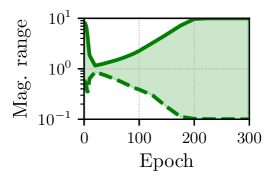
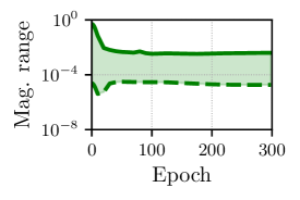
Model: SwinTransformer	Task: Classification	Dataset: ImageNet
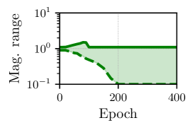
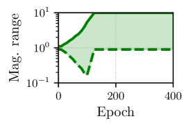
Model: EfficientNet	Task: Classification	Dataset: ImageNet

(a) Model-specific policy

Brightness	Contrast	Noise
Model: MobileNetv3	Task: Classification	Dataset: ImageNet
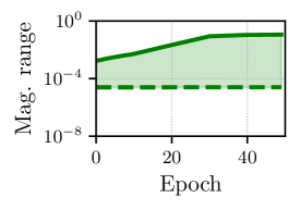
Model: MobileNetv3	Task: Segmentation	Dataset: ADE20k

(b) Task-specific policy

Figure 2: RangeAugment learns model- and task-specific policies. (a) shows magnitude ranges for two different models on the same task and dataset while (b) shows magnitude ranges for the same model on two different tasks. All models are trained end-to-end with RangeAugment. The target image similarity $\Delta$ (PSNR) is annealed from 40 to 5 in (a) and from 40 to 20 in (b). Training epochs and magnitude range (log scale) of augmentation operations are plotted in x- and y-axis respectively.

2 Related Work

Data augmentation combines different augmentation operations (e.g., random brightness, random contrast, random Gaussian noise, and data mixing) to synthesize additional training data. Traditional augmentation methods rely heavily on expert knowledge and extensive trial-and-error experiments. In practice, these manual augmentation methods have been used to train different models on a variety of datasets and tasks (e.g., Szegedy et al., 2015; He et al., 2016; Zhao et al., 2017; Howard et al., 2019). However, these policies may not be optimal for all models.

Motivated by neural architecture search (Zoph & Le, 2017), recent methods focus on finding optimal augmentation policies automatically from data. AutoAugment formulates automatic augmentation as a reinforcement learning problem, and uses model’s validation performance as a reward to find an augmentation policy leading to optimal validation performance. Because AutoAugment searches for several augmentation policy parameters, the search space is enormous and computationally intractable on large datasets and models. Therefore, in practice, policies found for smaller datasets are transferred to larger datasets. Since then, many follow-up works have focused on reducing the search space while delivering a similar performance to AutoAugment (Ratner et al., 2017; Lemley et al., 2017; LingChen et al., 2020; Li et al., 2020; Zheng et al., 2021; Liu et al., 2021a). The first line of research reduces the search time by introducing different hyper-parameter optimization methods, including population-based training (Ho et al., 2019), density matching (Lim et al., 2019; Hataya et al., 2020), and gradient matching (Zheng et al., 2021). The second line of research reduces the search space by making practical assumptions (Cubuk et al., 2020; Müller & Hutter, 2021). For instance, RandAugment (Cubuk et al., 2020) applies two transforms randomly with uniform probability. With these assumptions, RandAugment reduces AutoAugment’s search space from $10^{32}$ to $10^{2}$ while maintaining downstream networks performance.

One common characteristic among these different automatic augmentation methods is that they use fixed and manually-defined range of magnitudes for different augmentation operations, and focus on diversifying training data by using a large set of augmentation operations (e.g., 14 transforms). This is because the range of magnitudes for most augmentation operations is continuous and large, and searching over this large range is practically infeasible. Unlike these works, RangeAugment focuses on learning the magnitude range of each augmentation operation (Figs. 1 and 2). We show in Section 4 that RangeAugment is able to learn model- and task-specific policies while delivering competitive performance to previous automatic augmentation methods across different models.

3 RangeAugment

Existing automatic augmentation methods search for composite augmentations over a large set of augmentation operations, but each augmentation operation has a manually-defined range of magnitudes. This paper introduces RangeAugment, a method for learning a range of magnitude for each augmentation operation (Fig. 3). RangeAugment uses image similarity between the input and augmented image to learn the range of magnitudes for each augmentation operation. In the rest of this section, we first formulate the problem (Section 3.1), then elaborate on RangeAugment’s policy learning method (Section 3.2), then we give implementation details ( Section 3.3).

Figure 3: RangeAugment: End-to-end learning of model- and task-specific augmentation policy. The target image similarity value, $\Delta$, in RangeAugment controls the diversity of augmented samples. Therefore, the augmentation policy learning in RangeAugment reduces to linear search over discrete values of $\Delta$.

3.1 Problem Formulation

Let ${\mathcal{T}}=\{T_{1},\cdots,T_{N}\}$ be a set of $N$ differentiable augmentation operations. Each augmentation operation $T\in{\mathcal{T}}$ is parameterized by a scalar magnitude parameter $m\in\mathbb{R}$ such that ${T(\cdot;m):{\mathcal{X}}\rightarrow{\mathcal{X}}}$ is defined on the image space ${\mathcal{X}}$. Let $\pi_{\phi}$ be an augmentation policy that defines a distribution over sub-policies ${\mathcal{S}}\sim\pi_{\phi}$ in RangeAugment such that ${{\mathcal{S}}=\{T_{i}(\cdot;m_{i})\}_{i=1}^{N}}$. A sub-policy ${\mathcal{S}}$ applies augmentation operations to an input image ${\mathbf{x}}$ with uniform probability as

$${\mathcal{S}}({\mathbf{x}}):={\mathbf{x}}^{(N)},\quad{\mathbf{x}}^{(i)}=T_{i}({\mathbf{x}}^{(i-1)};m_{i}),\quad\quad{\mathbf{x}}^{(0)}={\mathbf{x}}.$$ (1)

For any given model and task, the goal of automatic augmentation is to find the augmentation policy $\pi_{\phi}$ that diversifies training data, and helps improve model’s generalization ability the most. RangeAugment learns the range of magnitudes for each augmentation operation in ${\mathcal{T}}$. Formally, the policy parameters in RangeAugment are $\phi=\{(a_{i},b_{i})\}_{i=1}^{N}$ and the magnitude parameter $m_{i}\sim U(a_{i},b_{i})$ for the $i$-th augmentation operation in a sub-policy ${\mathcal{S}}=\{T_{i}(\cdot;m_{i})\}_{i=1}^{N}$ is uniformly sampled, where $a_{i}\in\mathbb{R}$ and $b_{i}\in\mathbb{R}$ are learned parameters.

3.2 Policy learning

Diverse training data can be produced by using wider range of magnitudes, $(a_{i},b_{i})$, for each augmentation operation. However, directly searching for the optimal values of $(a_{i},b_{i})$ for each model and dataset is challenging because of its continuous nature. To address this, RangeAugment introduces an auxiliary loss which, in conjunction with the task-specific empirical loss, enables learning model-specific range of magnitudes for each augmentation operation in an end-to-end fashion.

Let $d:{\mathcal{X}}\times{\mathcal{X}}\rightarrow\mathbb{R}$ be a differentiable image similarity function that measures the similarity between the input and the augmented image. To control the range of magnitudes for each augmentation operation, RangeAugment minimizes the distance between the expected value of $d({\mathbf{x}},{\mathcal{S}}({\mathbf{x}}))$ and a target image similarity value $\Delta\in\mathbb{R}$ using an augmentation loss function $\mathcal{L}_{\text{ra}}$ (e.g., smooth L1 loss or L2 loss). An example of $d$ and $\Delta$ are peak signal to noise ratio (PSNR) and target PSNR value respectively. When target PSNR value is small, the difference between the input and augmented image obtained after applying an augmentation operation (say brightness) will be large. In other words, for a smaller target PSNR value, the range of magnitudes for brightness operation will be wider and vice-versa.

For a given value of $\Delta$ and parameterized model $f_{\theta}$ with parameters $\theta$, the overall loss function to learn model- and task-specific augmentation policy is a weighted sum of the augmentation loss $\mathcal{L}_{\text{ra}}$ and the task-specific empirical loss $\mathcal{L}_{\text{task}}$:

$$\theta^{*},\phi^{*}=\operatorname*{arg\,min}_{\theta,\phi}\mathbb{E}_{({\mathbf{x}},{\mathbf{y}})\sim{\mathcal{D}}_{\text{train}}}\left[\mathbb{E}_{{\mathcal{S}}\sim\pi_{\phi}}\left[\mathcal{L}_{\text{task}}(f_{\theta}({\mathcal{S}}({\mathbf{x}})),{\mathbf{y}})+\lambda\mathcal{L}_{\text{ra}}({\mathbf{x}},{\mathcal{S}}({\mathbf{x}});\Delta)\right]\right],$$ (2)

where $\lambda$ and ${\mathcal{D}}_{\text{train}}$ represent weight term and training set respectively. Note that, in Eq. 2, re-parameterization trick on uniform distributions (Kingma & Welling, 2013) is applied to back-propagate through the expectation over ${\mathcal{S}}\sim\pi_{\phi}$.

The $\Delta$ in Eq. 2 allows RangeAugment to control diversity of augmented samples. Therefore, the augmentation policy learning in RangeAugment reduces to searching a single scalar parameter, $\Delta$, that maximizes downstream model’s validation performance. RangeAugment finds the optimal value of $\Delta$ using a linear search.

3.3 Implementation details

We use PSNR as the image similarity function $d$ in our experiments because it is (1) a standard image quality metric, (2) differentiable, and (3) fast to compute. Across different downstream networks, we observe a 0.5%-3% training overhead over the empirical risk minimization baseline.

$m=0.1$	$m=1.0$	$m=10.0$

Figure 4: Example outputs of brightness operation, $T({\mathbf{x}};m)=m{\mathbf{x}}$, at different values of magnitude parameter $m$. At extremes (i.e., $m=0.1$ or $10$), the bus is hardly identifiable.

To find an optimal value of $\Delta$ in Eq. 2, we study two approaches: (1) fixed target PSNR ($\Delta\in\{5,10,20,30\}$) and (2) target PSNR with a curriculum, where the value of $\Delta$ is annealed from 40 to $\delta$ and $\delta\in\{5,10,20,30\}$. The learned ranges of magnitudes, $(a,b)$, can scale beyond the image space (e.g., negative values) and result in training instability. To prevent this, we clip the range of magnitudes if they are beyond extreme bounds of augmentation operations. We choose these extreme bounds such that objects in an image are hardly identifiable at or beyond the extreme points of the bounds (see Fig. 4). Also, because the focus of RangeAugment is to learn the range of magnitudes for each augmentation operation, we apply all augmentation operations in $\mathcal{T}$ with uniform probability. We use smooth L1 loss as augmentation loss function $\mathcal{L}_{\text{ra}}$.

To demonstrate the importance of magnitude ranges, we study RangeAugment with three basic operations (brightness, contrast, and additive Gaussian noise), and show empirically in Section 4 that RangeAugment can achieve competitive performance to existing methods with 4 to 5 times fewer augmentation operations.

4 Evaluating RangeAugment on Image Classification

RangeAugment can learn model-specific augmentation policies. To evaluate this, we first study the importance of single and composite augmentation operations using ResNet-50 on the ImageNet dataset (Section 4.2). We then study model-level generalization of RangeAugment (Section 4.3).

4.1 Experimental Set-up

Dataset

For image classification, we use the ImageNet dataset that has 1.28M training and 50k validation images spanning across 1000 categories. We use top-1 accuracy to measure performance.

Baseline models

To evaluate the effectiveness of RangeAugment, we study different CNN- and transformer-based models. We group these models into two categories based on their complexity: (1) mobile: MobileNetv1 (Howard et al., 2017), MobileNetv2 (Sandler et al., 2018), MobileNetv3 (Howard et al., 2019), and MobileViT (Mehta & Rastegari, 2021) and (2) non-mobile: ResNet-50 (He et al., 2016), ResNet-101, EfficientNet (Tan & Le, 2019), and SwinTransformer (Liu et al., 2021b). We implement RangeAugment using the CVNets library (Mehta et al., 2022) and use their baseline model implementations and training recipes. Additional experiments, including the effect of individual and joint learning on RangeAugment’s performance, along with training details are given in Appendices A and D.1 respectively.

Baseline augmentation methods

For an apples to apples comparison, each baseline model is trained with three different random seeds and the following baseline augmentation strategies: (1) Baseline - standard Inception-style pre-processing (random resized cropping and random horizontal flipping) (Szegedy et al., 2015), (2) RandAugment - Baseline pre-processing followed by RandAugment policy of Cubuk et al. (2020), (3) AutoAugment - Baseline pre-processing followed by AutoAugment policy of Cubuk et al. (2019), and (4) RangeAugment - Baseline pre-processing following by the proposed augmentation policy in Section 3. See Section 4.4 for comparison with other augmentation methods.

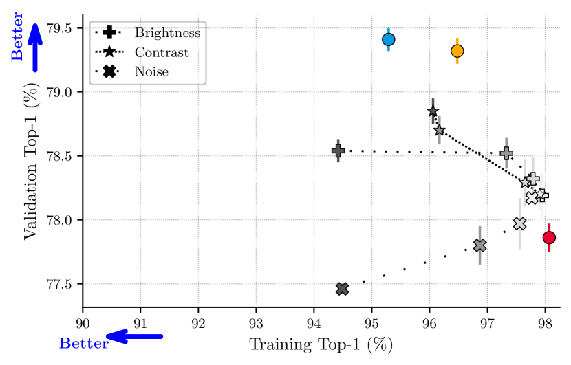
(a) $N=1$

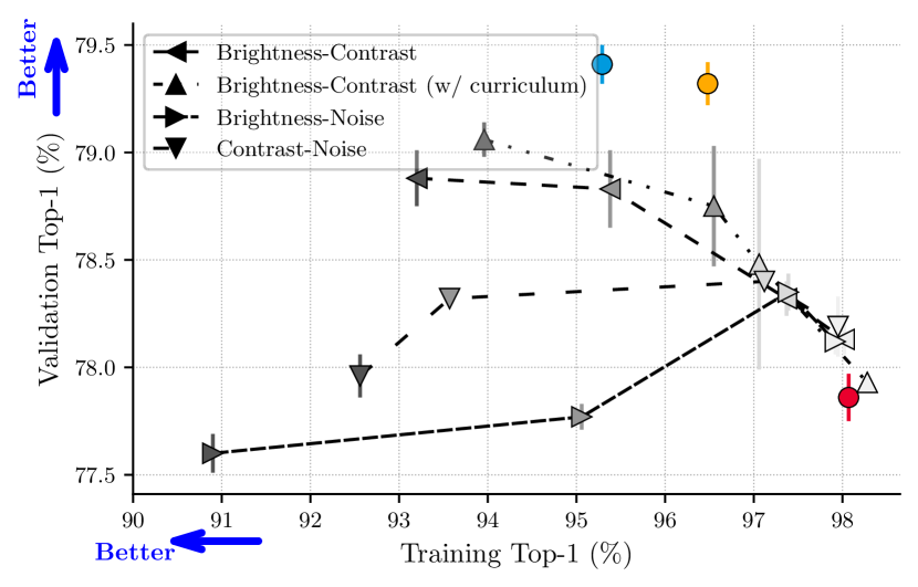
(b) $N=2$

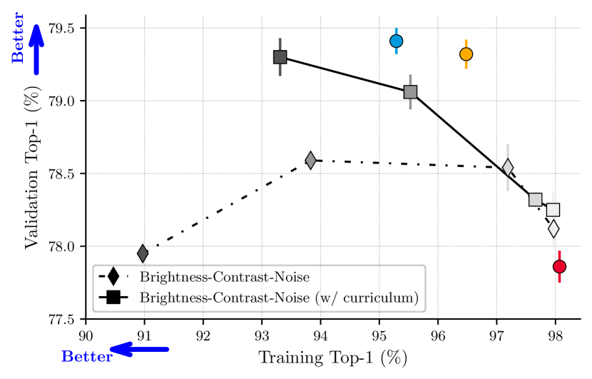
(c) $N=3$

Figure 5: Augmentation operation characterization for ResNet-50 using RangeAugment. In (a-c), the performance of ResNet-50 on the ImageNet dataset is shown when data diversity is increased by learning the range of magnitudes for single ($N=1$) and composite augmentation operations ($N>1$) using RangeAugment. For curriculum learning, target PSNR value is annealed from 40 to the value mentioned in the legend. For generalization, we are interested in the gap between training and validation accuracy (Jiang et al., 2020). Given two models with similar validation accuracy, the model with a larger gap between training and validation accuracy demonstrates better generalization as training is much harder for this model.

$\Delta$	Brightness	Contrast	Noise
$5$
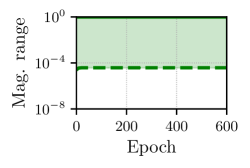
$15$

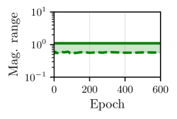
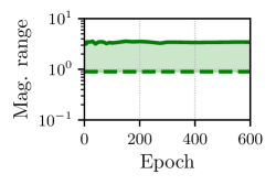
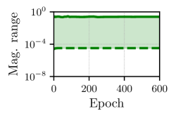
(a) $N=1$ (without curriculum)

$\Delta$	Brightness	Contrast	Noise
5
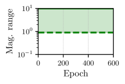
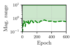
15

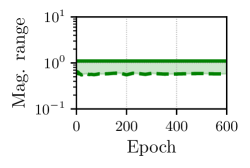
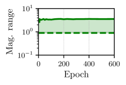
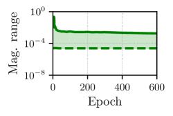
(b) $N=3$ (without curriculum)

$\Delta$	Brightness	Contrast	Noise
$40\rightarrow 5$
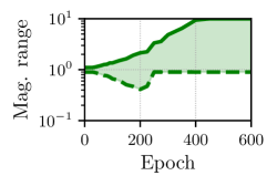
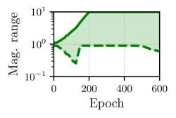
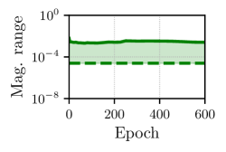
$40\rightarrow 15$

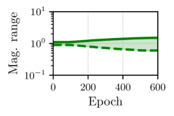
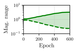
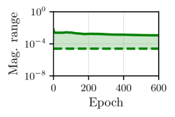
(c) $N=3$ (with curriculum)

Figure 6: Learned range of magnitudes for different augmentation operations when training ResNet-50 jointly with RangeAugment. In (a) and (b), the target image similarity value (PSNR; $\Delta$) is fixed while in (c), $\Delta$ is annealed using cosine curriculum. Training epochs and magnitude range (log scale) of augmentation operations are plotted in x- and y-axis respectively.

4.2 Augmentation Operation Characterization using RangeAugment

The quantity and diversity of training data can be increased by (1) increasing the magnitude range of each augmentation operation and (2) composite augmentation operations. Fig. 5 characterizes the effect of these variables on ResNet-50’s performance on the ImageNet dataset. We can make the following observations:

1. Single augmentation operation improves baseline accuracy. Fig. 6(a) shows that single augmentation operation ($N=1$) with wider magnitude ranges (e.g., the range of magnitudes at target PSNR of 5 are wider than the ones at target PSNR of 15) helped in improving ResNet-50’s validation accuracy and reducing training accuracy, thereby improving its generalization capability (Fig. 5(a)). Particularly, increasing the magnitude range of contrast (or brightness) operation increased ResNet-50’s validation performance over baseline by 1.0% (or 0.7%) while decreasing the training performance by 2% (or 3%). This is likely because wider magnitude ranges of an augmentation operation increases diversity of training data. On the other hand, the additive Gaussian noise operation with a wider magnitude range slightly dropped the validation accuracy, but still reduces the training accuracy. In other words, it improves ResNet-50’s generalization ability.

2. Composite augmentation operations improve model’s generalization. Composite augmentation operations ($N>1$; Figs. 5(b) and 5(c)) reduces the training accuracy significantly while having a validation performance similar to single augmentation operation. This is expected as composite operations further increases training data diversity.

3. Curriculum matters. Fig. 6(c) shows that progressively learning to increase the diversity of augmented samples (i.e., narrower to wider magnitude ranges) using a cosine curriculum further improves the performance (Fig. 5(c)). A plausible explanation is that the learned magnitude ranges of different augmentation operations using RangeAugment with fixed target PSNR may get stuck near poor solutions. Because the range of magnitudes are wider for these solutions (e.g., the range of magnitudes at target PSNR value of 5 in Fig. 6(a) & Fig. 6(b)), RangeAugment samples more diverse data from the beginning of the training, making training difficult. Gradually annealing target PSNR from high to low (e.g., 40 to 5 in Fig. 6(c)) allows RangeAugment to increase the data diversity slowly, thereby helping model to learn better representations. Importantly, it also allows RangeAugment to identify useful ranges for each augmentation operation. For example, the range of magnitudes for the additive Gaussian noise operation is relatively narrower when optimizing with curriculum (e.g., annealing target PSNR from 40 to 5; Fig. 6(c)) compared to optimizing with a fixed target PSNR of 5 (Fig. 6(b)). This indicates that noise operation with narrow magnitude range is favorable for training ResNet-50 on the ImageNet classification task. This concurs with results in Figs. 5(a) and 5(b) where we observed that noise operation does not improve ResNet-50’s validation performance. Moreover, our findings with progressively increasing data diversity are consistent with previous works (e.g., Bengio et al., 2009; Tan & Le, 2021) that shows scheduling training samples from easy to hard helps improve model’s performance.

   Interestingly, ResNet-50 with RangeAugment ($N=3$) achieves comparable validation accuracy and a smaller generalization gap as compared to state-of-the-art methods which use more augmentation operations ($N>14$) to increase data diversity during training. We conjecture that the difference in the generalization gap between existing methods and RangeAugment is probably caused by insufficient policy search in existing methods as they use manually-defined magnitude ranges for each augmentation operation during search.

In the rest of experiments, we will use all three augmentations ($N=3$) with cosine curriculum.

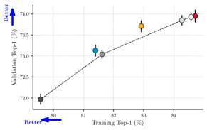
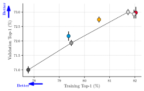
MobileNetv1	MobileNetv2
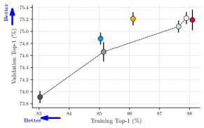
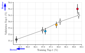
MobileNetv3	MobileViT

(a) Mobile models

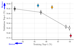
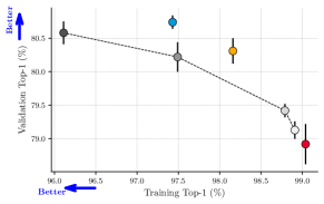
ResNet-50	ResNet-101
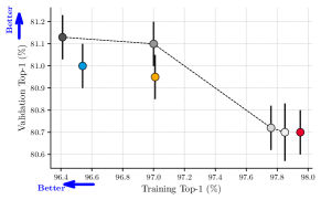
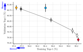
EfficientNet-B3	SwinTransformer-Tiny

(b) Non-mobile models

Figure 7: RangeAugment is model agnostic. Performance of different models on the ImageNet dataset using RangeAugment. Here, the target PSNR value is annealed from 40 to the value mentioned in the legend.

4.3 Model-level Generalization of RangeAugment

Fig. 5 shows RangeAugment is effective for ResNet-50. Natural questions that arise are:

1. Can RangeAugment be applied to other vision models? RangeAugment’s seamless integration ability with little training overhead (0.5% to 3%) over the baseline model allows us to study the generalization capability of different vision models easily. Fig. 7 shows the performance of different models with RangeAugment. When data regularization is increased for mobile models by decreasing the target PSNR value from 40 to 5, the training as well as validation accuracy of different mobile models is decreased significantly as compared to the baseline. This is likely because of the limited capacity of these models. On the other hand, data regularization improved the performance of non-mobile models significantly. Consistent with our observations for ResNet-50 in Fig. 5, we found that non-mobile models trained with RangeAugment are able to achieve competitive performance to state-of-the-art automatic augmentation methods, such as AutoAugment ($N=16$), but with fewer augmentations ($N=3$).

2. Does RangeAugment learn architecture-specific augmentations? Fig. 2(a) shows the learned magnitude ranges for different augmentation operations for a transformer- (SwinTransformer) and a CNN-based (EfficientNet) model. Though both of these architectures use the same curriculum in RangeAugment (i.e., target PSNR is annealed from 40 to 5), they learn different magnitude ranges for each augmentation operation. This shows that RangeAugment is capable of learning model-specific magnitude ranges for each augmentation operation.

3. Does RangeAugment increase variance on model performance? Because of the stochastic training and presence of randomness during different stages of training including RangeAugment, there may be some variability in model’s performance. To measure the variability in model’s performance, we run each experiment with three different random seeds. For different models, the standard deviation of model’s validation accuracy in Fig. 7 is between $0.01$ and $0.2$, and is in accordance with previous works on the ImageNet dataset (Radosavovic et al., 2020; Wightman et al., 2021). These results show that training models with RangeAugment leads to a stable model performance.

4.4 Comparison with Existing Methods

Comparison for ResNet-50

Most previous automatic augmentation methods use ResNet-50 as a baseline model. For apples to apples comparison, we train ResNet-50 with different augmentation methods using the same training recipe (Section D.1). Table 2 shows that RangeAugment achieves similar performance as previous methods, but with $4-5\times$ fewer augmentation operations. Note that, unlike previous methods, the search space of RangeAugment is independent of the augmentation operations and is constant (Table 1(a) and Fig. 1).

Aug. method	# of operations	Top-1 accuracy
AutoAugment (Cubuk et al., 2019)	16	77.6%
RandAugment Cubuk et al. (2020)	14	77.6%
Fast AutoAugment (Dollár et al., 2021)	16	77.6%
TrivialAugment (Müller & Hutter, 2021)	14	78.1%
Deep AutoAugment (Zheng et al., 2022)	16	78.3%
RandAugment + MixUp (Wightman et al., 2021)	14 + 2	80.4%
RandAugment + MixUp + RandonErase (Touvron et al., 2021)	14 + 2 + 1	79.5%
AutoAugment + MixUp (Touvron et al., 2019)	16 + 2	79.5%
AutoAugment + Mixup (Our repro.)	16 + 2	80.2%
RandAugment + Mixup (Our repro.)	14 + 2	80.4%
TrivialAugment + Mixup (Our repro.)	14 + 2	80.4%
Deep AutoAugment + Mixup (Our repro.)	16 + 2	80.1%
RangeAugment + Mixup (Ours)	3 + 2	80.2%

Table 2: Accuracy of ResNet-50 on the ImageNet validation set. RangeAugment compares favorably to previous methods, but with $4-5\times$ fewer augmentation operations. Best results within ImageNet’s standard deviation range of $\pm 0.2$ are highlighted in bold.

Model	Source	Data augmentation methods			Top-1
		Auto aug. method	Random erase	Mixup	accuracy
Mobile models
MobileNetV1-1.0	Orig. (Howard et al., 2017)	✗	✗	✗	70.6%
	Our repro.	RandAugment ($N=14$)	✗	✗	73.7%
	Our repro.	AutoAugment ($N=16$)	✗	✗	73.1%
	Ours	RangeAugment ($N=3$)	✗	✗	73.8%
MobileNetV2-1.0	Orig. (Sandler et al., 2018)	✗	✗	✗	72.0%
	Our repro.	RandAugment ($N=14$)	✗	✗	72.7%
	Our repro.	AutoAugment ($N=16$)	✗	✗	72.1%
	Ours	RangeAugment ($N=3$)	✗	✗	73.0%
MobileNetV3-Large	Orig. (Howard et al., 2019)	✗	✗	✗	74.6%
	Our repro.	RandAugment ($N=14$)	✗	✗	75.2%
	Our repro.	AutoAugment ($N=16$)	✗	✗	74.9%
	Ours	RangeAugment ($N=3$)	✗	✗	75.1%
MobileViT-Small	Orig. (Mehta & Rastegari, 2021)	✗	✗	✗	78.4%
	Our repro.	RandAugment ($N=14$)	✗	✗	77.9%
	Our repro.	AutoAugment ($N=16$)	✗	✗	77.7%
	Ours	RangeAugment ($N=3$)	✗	✗	78.2%
Non-mobile models
ResNet-50	Orig. (He et al., 2016)	✗	✗	✗	76.2%
	TIMM (Wightman et al., 2021)	RandAugment ($N=14$)	✗	✓	80.4%
	Our repro.	RandAugment ($N=14$)	✗	✓	80.4%
	Our repro.	AutoAugment ($N=16$)	✗	✓	80.2%
	Ours	RangeAugment ($N=3$)	✗	✓	80.2%
ResNet-101	Orig. (He et al., 2016)	✗	✗	✗	77.4%
	TIMM (Wightman et al., 2021)	RandAugment ($N=14$)	✗	✓	81.5%
	Our repro.	RandAugment ($N=14$)	✗	✓	81.4%
	Our repro.	AutoAugment ($N=16$)	✗	✓	81.6%
	Ours	RangeAugment ($N=3$)	✗	✓	82.0%
EfficientNet-B0	Orig. (Tan & Le, 2019)	AutoAugment ($N=16$)	✓	✓	77.1%
	TIMM (Wightman et al., 2021)	RandAugment ($N=14$)	✗	✓	77.0%
	Our repro.	RandAugment ($N=14$)	✗	✓	77.0%
	Our repro.	AutoAugment ($N=16$)	✗	✓	77.1%
	Ours	RangeAugment ($N=3$)	✗	✓	77.3%
EfficientNet-B1	Orig. (Tan & Le, 2019)	AutoAugment ($N=16$)	✓	✓	79.1%
	TIMM (Wightman et al., 2021)	RandAugment ($N=14$)	✗	✓	79.2%
	Our repro.	RandAugment ($N=14$)	✗	✓	79.0%
	Our repro.	AutoAugment ($N=16$)	✗	✓	79.2%
	Ours	RangeAugment ($N=3$)	✗	✓	79.5%
EfficientNet-B2	Orig. (Tan & Le, 2019)	AutoAugment ($N=16$)	✓	✓	80.1%
	TIMM (Wightman et al., 2021)	RandAugment ($N=14$)	✗	✓	80.4%
	Our repro.	RandAugment ($N=14$)	✗	✓	80.8%
	Our repro.	AutoAugment ($N=16$)	✗	✓	80.9%
	Ours	RangeAugment ($N=3$)	✗	✓	81.3%
EfficientNet-B3	Orig. (Tan & Le, 2019)	AutoAugment ($N=16$)	✓	✓	81.6%
	TIMM (Wightman et al., 2021)	RandAugment ($N=14$)	✗	✓	81.4%
	Our repro.	RandAugment ($N=14$)	✗	✓	81.5%
	Our repro.	AutoAugment ($N=16$)	✗	✓	81.2%
	Ours	RangeAugment ($N=3$)	✗	✓	81.9%
Swin-Tiny	Orig. (Liu et al., 2021b)	RandAugment ($N=14$)	✓	✓	81.3%
	Our repro.	RandAugment ($N=14$)	✗	✓	80.8%
	Our repro.	AutoAugment ($N=16$)	✗	✓	81.0%
	Ours	RangeAugment ($N=3$)	✗	✓	81.1%
Swin-Small	Orig. (Liu et al., 2021b)	RandAugment ($N=14$)	✓	✓	83.0%
	Our repro.	RandAugment ($N=14$)	✗	✓	82.7%
	Our repro.	AutoAugment ($N=16$)	✗	✓	82.7%
	Ours	RangeAugment ($N=3$)	✗	✓	82.8%

Table 3: RangeAugment is competitive to previous methods. As per our observations in Section 4.1, we anneal $\Delta$ from 40 to 30 and 40 to 5 for mobile and non-mobile models respectively. Methods whose performance is within ImageNet’s standard deviation range of $\pm 0.2$ of the best model are highlighted in bold. Here, $N$ denotes the number of augmentation operations. We reproduce models with RangeAugment and AutoAugment to align low-level details.

Comparison with other models

To demonstrate the effectiveness of RangeAugment across different models, we compare with AutoAugment and RandAugment. This is because (1) most state-of-the-art models use either RandAugment or AutoAugment along with Mixup transforms (Zhang et al., 2018; Yun et al., 2019) and (2) different augmentation methods deliver similar performance (Table 2). Table 3 shows that RangeAugment delivers competitive performance to existing automatic methods with significantly fewer augmentation operations.

5 Task-level Generalization of RangeAugment

Section 4 shows the effectiveness of RangeAugment on different downstream models on the ImageNet dataset. However, one might ask whether RangeAugment can be used for tasks other than image classification. To evaluate this, we study RangeAugment different tasks: (1) semantic segmentation (Section 5.1), (2) object detection (Section 5.2), (3) foundation models (Section 5.3), and (4) knowledge distillation (Section 5.4).

5.1 Semantic Segmentation with DeepLabv3 on ADE20k

Dataset and baseline models

We use the ADE20k dataset (Zhou et al., 2017) that has 20k training and 2k validation images across 150 semantic classes. We report the segmentation performance in terms of mean intersection over union (mIoU) on the validation set.

We integrate mobile and non-mobile classification models with the Deeplabv3 segmentation head (Chen et al., 2018) and finetune each model for 50 epochs. See Section D.1 for training details. We do not study SwinTransformer for semantic segmentation because it is not compatible with Deeplabv3’s segmentation head design as it adjusts the atrous rate of convolutions to control the output stride of backbone network.

Baseline augmentation methods

For semantic segmentation, experts have hand-crafted augmentation policies, and these manual policies are used to train state-of-the-art semantic segmentation methods (e.g., Chen et al., 2017; Zhao et al., 2017; Xie et al., 2021; Liu et al., 2021b). For an apples to apples comparison, we train each segmentation model with three different random seeds and compare with the following baselines: (1) Baseline - standard pre-processing (randomly resize short image dimension, random horizontal flip, and random crop), (2) Manual - baseline pre-processing with hand-crafted augmentation operations (color jittering using photometric distortion, random rotation, and random Gaussian noise), and (3) RangeAugment - baseline pre-processing with learnable range of magnitudes for brightness, contrast, and noise (i.e., $N=3$). For reference, we include DeepLabv3 results (if available) from a popular segmentation library (MMSegmentation, 2020).

Comparison with segmentation-specific augmentation methods

Table 4(a) shows that RangeAugment improves the performance of different models in comparison to other augmentation methods. Interestingly, for semantic segmentation, the magnitude range of additive Gaussian noise is wider compared to image classification (Fig. 2(b)). This concurs with previous manual augmentation methods which also found that Gaussian noise is important for semantic segmentation (Zhao et al., 2017; Asiedu et al., 2022). Overall, these results suggest that RangeAugment learns task-specific augmentation policies.

DeepLabv3 strikes back

Tables 4(b) and 4(c) shows that RangeAugment improves the performance of DeepLabv3 significantly across different backbones, and is able to deliver better performance than UPerNet (Xiao et al., 2018), which has been widely adopted for semantic segmentation tasks in recent state-of-the-art models, including ConvNext (Liu et al., 2022).

Backbone	Augmentation method
	Baseline	Manual	RangeAugment (Ours)
			(40, 5)	(40, 10)	(40, 20)	(40, 30)
MobileNetv1	38.77 $\pm$ 0.20	38.12 $\pm$ 0.16	36.46 $\pm$ 0.19	38.20 $\pm$ 0.26	38.96 $\pm$ 0.34	39.37 $\pm$ 0.19
MobileNetv2	37.74 $\pm$ 0.29	37.10 $\pm$ 0.27	35.58 $\pm$ 0.30	37.43 $\pm$ 0.73	38.06 $\pm$ 0.17	38.23 $\pm$ 0.36
MobileNetv3	37.58 $\pm$ 0.67	36.68 $\pm$ 0.34	34.80 $\pm$ 0.16	36.54 $\pm$ 0.12	37.77 $\pm$ 0.24	38.10 $\pm$ 0.13
MobileViT	37.69 $\pm$ 0.50	37.19 $\pm$ 0.47	35.04 $\pm$ 0.83	36.70 $\pm$ 0.19	37.94 $\pm$ 0.45	38.41 $\pm$ 0.22
ResNet-50	42.27 $\pm$ 0.54	43.29 $\pm$ 0.27	41.56 $\pm$ 0.21	42.95 $\pm$ 0.22	43.31 $\pm$ 0.16	43.00 $\pm$ 0.28
ResNet-101	43.29 $\pm$ 0.17	44.04 $\pm$ 0.52	43.22 $\pm$ 0.52	43.89 $\pm$ 0.43	44.77 $\pm$ 0.28	43.95 $\pm$ 0.31
EfficientNet-B3	40.86 $\pm$ 0.55	41.15 $\pm$ 0.65	39.42 $\pm$ 0.29	40.39 $\pm$ 0.48	41.43 $\pm$ 0.36	41.08 $\pm$ 0.36
ResNet-50⋆	42.57 $\pm$ 0.43	43.49 $\pm$ 0.21			43.90 $\pm$ 0.10
ResNet-101⋆	44.19 $\pm$ 0.17	45.24 $\pm$ 0.27			46.42 $\pm$ 0.19
EfficientNet-B3⋆	41.19 $\pm$ 0.16	42.35 $\pm$ 0.35			43.68 $\pm$ 0.16

(a) RangeAugment vs. segmentation-specific manual augmentation methods. All models are reproduced by us to align low-level implementation details. Here, ^⋆ indicates that these backbones are trained with RangeAugment and mixup transforms.

Backbone	Seg. architecture	mIoU
MobileNetv2	DeepLabv3†	34.0
	PSPNet‡	35.8
	DeepLabv3 (Our repro.)	$37.74\pm 0.29$
	DeepLabv3 w/ RangeAugment (Ours)	$\mathbf{38.23\pm 0.36}$
ResNet-50	UPerNet‡	40.4
	UPerNet†	42.1
	PSPNet†	42.5
	DeepLabv3†	42.7
	DeepLabv3 (Our repro.)	$43.49\pm 0.21$
	DeepLabv3 w/ RangeAugment (Ours)	$\mathbf{43.90\pm 0.10}$
ResNet-101	UPerNet‡	42.0
	PSPNet†	42.5
	UPerNet†	43.8
	DeepLabv3†	45.0
	DeepLabv3 (Our repro.)	$45.24\pm 0.27$
	DeepLabv3 w/ RangeAugment (Ours)	$\mathbf{46.42\pm 0.19}$

(b) Comparison with different architectures for the same backbone. ^† and ^‡ represents that these results are from MMSeg (MMSegmentation, 2020) and CSAIL (Zhou et al., 2017) segmentation libraries, respectively. Our training schedules, including batch size, are similar to MMSeg and CSAIL.

Seg. model	# Params.	FLOPs	mIoU
Swin w/ UPerNet (Liu et al., 2021b)	60 M	945 G	45.8
ConvNext w/ UPerNet (Liu et al., 2022)	60 M	939 G	46.7
ResNet-101 w/ DeepLabv3 (RangeAugment; ours)	77 M	303 G	$\mathbf{46.42\pm 0.19}$

(c) Comparison with recent segmentation models

Table 4: Semantic segmentation on the ADE20k dataset.

Backbone	mIoU	Prev. best
MobileNetV1	77.2	–
MobileNetV2	76.7	75.3 (Sandler et al., 2018)
MobileNetv3	77.0	–
EfficientNet-B3	82.0	–
ResNet-50	81.2	–
ResNet-101	84.0	82.7† (Chen et al., 2017)

Table 5: RangeAugment’s curriculum are transferable from ADE20k to PASCAL VOC. Here, each backbone is trained with DeepLabv3 and RangeAugment. For mobile backbones, $\Delta$ is annealed from 40 to 30 while for non-mobile backbones, $\Delta$ is annealed from 40 to 20 (as noted in Table 4(a)). ^†Model is evaluated with multiple scales and left-right flips during inference. Here, – represents that results are not available.

RangeAugment’s curriculum is transferable to other segmentation datasets

Table 4(a) shows that mobile and non-mobile backbones prefer different curriculum for the task of semantic segmentation. For mobile models, annealing the value of $\Delta$ from 40 to 30 yields best results while for non-mobile models, annealing the value of $\Delta$ from 40 to 20 yields the best results. Can we use the same curriculum for semantic segmentation on other datasets? To validate this, we train DeepLabv3 with different backbones on the PASCAL VOC dataset (Everingham et al., 2010). Table 5 shows that RangeAugment’s curriculum are transferable from ADE20k to PASCAL VOC.

5.2 Object detection with Mask R-CNN on MS-COCO

Dataset and baseline models

We use MS COCO dataset (Lin et al., 2014) that has about 118k training and 5k validation images across 81 catogries (including background). We report the instance detection and segmentation performance in terms of standar COCO mean average precision (mAP) on the validation set.

We integrate mobile and non-mobile backbones with the Mask R-CNN (He et al., 2017). Following Detectron2 (Wu et al., 2019) which finetunes Mask R-CNN for about 270k iterations, we also finetune our model for similar number of iterations (230k iterations) with multi-scale sampler of (Mehta & Rastegari, 2021).

Baseline augmentation methods

We study Mask R-CNN with two augmentation methods: (1) Baseline - standard image resizing as in (He et al., 2017), and (2) RangeAugment - standard image resizing with learnable range of magnitudes for brightness, contrast, and noise.

Searching for the curriculum

We train Mask R-CNN with ResNet-50 for different target image similarity value, $\Delta$. Fig. 8(a) shows that Mask R-CNN achieves the best performance when we anneal $\Delta$ from 40 to 10.

Transferring curriculum to other backbones

We integrate different backbones with Mask R-CNN and finetune it by annealing $\Delta$ from 40 to 10. Fig. 8(b) shows that RangeAugment improves the detection performance across backbones significantly.

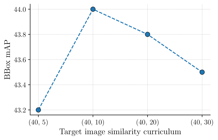
(a)

Backbone	mAP (w/o RangeAugment)			mAP (w/ RangeAugment)
	BBox	Segm		BBox	Segm
Mobile backbones
MobileNetv1	38.2	34.5		39.4	35.6
MobileNetv2	37.7	34.1		38.4	34.7
MobileNetv3	35.1	31.9		35.6	32.5
MobileViT	40.9	36.7		42.0	37.7
Non-mobile backbones
EfficientNet-B3	44.0	39.0		44.5	39.5
ResNet-50	43.4	39.0		44.0	39.5
ResNet-101	45.5	40.5		46.1	41.1

(b)

Figure 8: Enhanced object detection results of Mask R-CNN with RangeAugment on COCO dataset. (a) Effect of varying the target image similarity curriculumn on the performance of Mask R-CNN with ResNet50. Annealing the PSNR value from 40 to 10 yields best performance. (b) Effect of transferring the best curriculum in (a) to different backbones. We observe that RangeAugment improves detection performance across backbones. All models are trained by us to align low-level implementation details.

5.3 Learning Augmentation for Foundation Models at Scale

A common perception in the community is that training on extremely large datasets does not require data augmentation (Radford et al., 2021; Zhai et al., 2022). In this section, we challenge this perception and shows that RangeAugment improves the accuracy and data efficiency of large scale foundation models.

Dataset and baseline models

We train the CLIP (Radford et al., 2021) model with two different dataset sizes (304M and 1.1B image-text pairs) and evaluate their 0-shot top-1 accuracy on ImageNet’s validation set using the same language prompts as as OpenCLIP (Ilharco et al., 2021).

We train CLIP (Radford et al., 2021) with RangeAugment from scratch (Section D.1). The model uses ViT-B/16 (or ViT-H/16) (Dosovitskiy et al., 2020) as its image encoder and transformer as its text encoder, and minimizes contrastive loss during training. We use multi-scale sampler of Mehta et al. (2022) to make CLIP more robust to input scale changes. Because less data regularization is required at a scale of 100M+ samples, we anneal the target PSNR in RangeAugment from 40 to 20. We compare the performance with CLIP and OpenCLIP.

Results

Table 6 compares the zero-shot performance of different models. Compared to OpenCLIP, RangeAugment achieves (1) 1.2% better accuracy for similar dataset size and (2) similar accuracy with $2\times$ fewer data samples. This shows that RangeAugment is effective when training foundation models on large-scale datasets.

Model	Dataset size	Test resolution	Top-1 Accuracy (%)
CLIP of Radford et al. (2021)	400M	$224\times 224$	68.3%
OpenCLIP of Ilharco et al. (2021)	400M	$224\times 224$	67.1%
CLIP w/ RangeAugment (Ours)	302M (1.1B)	$160\times 160$	65.8% (69.2%)
		$192\times 192$	67.4% (71.1%)
		$224\times 224$	68.3% (71.9%)
		$256\times 256$	68.8% (72.4%)
		$288\times 288$	69.0% (72.8%)

(a) ViT-B/16 (Network parameters: 150M)

Model	Dataset size	Test resolution	Top-1 Accuracy (%)
OpenCLIP of Ilharco et al. (2021)	2.0B	$224\times 224$	78.0%
CLIP w/ RangeAugment (Ours)	1.1B	$160\times 160$	76.1%
		$192\times 192$	77.4%
		$224\times 224$	77.9%
		$256\times 256$	78.4%
		$288\times 288$	78.6%

(b) ViT-H/16 (Network parameters: 756M)

Table 6: RangeAugment learns augmentation efficiently for foundation models at scale. With RangeAugment, we (a) improve accuracy by 1.2% for similar dataset size and (b) achieve similar accuracy with approx. $2\times$ fewer data samples as compared to OpenCLIP. Each entry of CLIP with RangeAugment is the same model, but evaluated at different resolutions. Results within parenthesis in (a) are for CLIP ViT-B/16 when trained on 1.1B image-text pairs.

5.4 Learning Augmentation for Student Model during Distillation

Besides empirical risk minimization (ERM), another popular approach for training accurate mobile models is knowledge distillation (KD). In a standard distillation set-up, student and teacher receives the same input augmentations. Also, because of low complexity of mobile models, the augmentation strength is less. Because teachers are trained with extensive augmentations, it remains an open question to find an optimal range of magnitudes for students. This section shows that RangeAugment can be used to learn the magnitude range for student model.

Dataset and teacher details

We distill knowledge from ResNet-101 to mobile models on the task of image classification on the ImageNet dataset. We use the same hyper-parameters during distillation as the ERM models.

Searching for the curriculum

We distill knowledge from ResNet-101 to MobileNetv1 on the ImageNet dataset at different target image similarity values, $\Delta$. Fig. 9(a) shows that MobileNetv1 achieves the best performance when we anneal $\Delta$ from 40 to 20. This curriculum is different from our observations in Table 3, where we found that MobileNetv1 trained with ERM achieve best performance when we anneal $\Delta$ from 40 to 30. Moreover, Fig. 9(c) shows that MobileNetv1 prefers wider magnitude ranges during KD as compared to ERM.

RangeAugment’s curriculum is transferable for other mobile models

To see if the curriculum found for MobileNetv1 for KD is transferrable to other mobile backbones, we distilled knowledge from ResNet-101 to other backbones. During distillation, we annealed the $\Delta$ from 40 to 20. Fig. 9(b) shows that KD with RangeAugment improves the performance of different models.

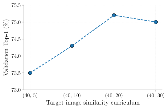
(a)

Model	Top-1 Accuracy
	ERM	KD
MobileNetv1	73.8%	75.2%
MobileNetv2	73.0%	73.4%
MobileNetv3	75.1%	76.0%
MobileViT	78.2%	79.4%

(b)

$\Delta$	Brightness	Contrast	Noise
MobileNetv1 trained using ERM (ImageNet Top-1: 73.8%)
$40\rightarrow 30$
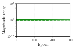
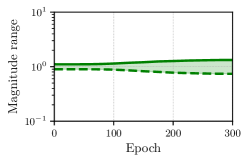
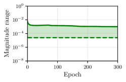
MobileNetv1 trained using KD (ImageNet Top-1: 75.2%)
$40\rightarrow 20$

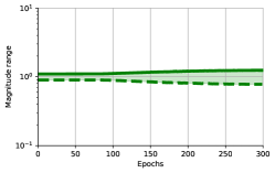
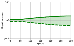
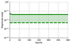
(c)

Figure 9: RangeAugment learns the magnitude range of augmentation operations for the task of distillation. In (a), we search for the curriculum for target image similarity value. Here, student is MobileNetv1 and teacher is ResNet-101. In (b), we distill knowledge from ResNet-101 to different mobile backbones. We use the same curriculum values that gives the best accuracy in (a); demonstrating the curriculum is transferable. In (c), we visualize the magnitude range of different augmentation operations for the MobileNetv1 model trained with ERM and KD. During distillation, MobileNetv1 preferred wider magnitude ranges as compared to ERM.

6 Conclusion

This paper introduces an end-to-end method for learning model- and task-specific automatic augmentation policies with a constant search time. We demonstrated that RangeAugment delivers competitive performance to existing methods across different downstream models and tasks. This is despite the fact that RangeAugment uses only three basic augmentation operations as opposed to a large set of complex augmentation operations in existing methods. These results underline the importance of magnitude range of augmentation operations in automatic augmentation. We also showed that RangeAugment can be seamlessly integrated with other tasks and achieve similar or better performance than existing methods.

Future work

We plan to apply RangeAugment to learn the range of magnitudes for complex augmentation operations (e.g., geometric transformations) using different image similarity functions (e.g., SSIM). In addition to learning the range of magnitudes of each augmentation operation, we plan to apply RangeAugment to learn how to compose different augmentation operations with a constant search time.

Appendix A Ablations on the ImageNet dataset

In this section, we study different components of RangeAugment using ResNet-50. For learning augmentation policy, we anneal the target image similarity (PSNR) value $\Delta$ from 40 to 5.

Effect of different curriculum

We trained RangeAugment with two curriculum’s: (1) linear and (2) cosine. We found that cosine curriculum delivers 0.1-0.2% better performance than linear. Therefore, we use cosine curriculum.

Effect of $\lambda$

The weight term, $\lambda$, in Eq. 2 allows RangeAugment to balance the trade-off between augmentation loss $\mathcal{L}_{\text{ra}}$ and empirical loss $\mathcal{L}_{\text{task}}$. To study its impact, we vary the value of $\lambda$ from 0.0 to 0.15. Empirical results in Fig. 10 shows that the good range for $\lambda$ is between 0.0006 and $0.002$. In our experiments, we use $\lambda=0.0015$.

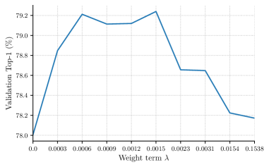
Figure 10: Effect of weight term, $\lambda$, on ResNet-50’s performance on the ImageNet dataset.

$\Delta$	Brightness	Contrast	Noise
$40\rightarrow 5$
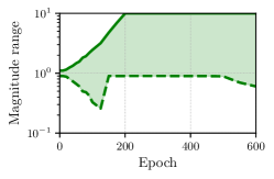
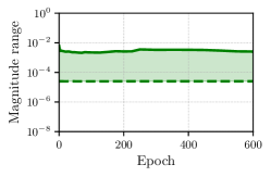
Joint loss
$40\rightarrow 5$
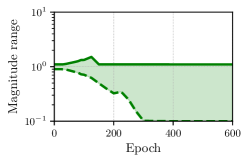
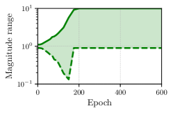
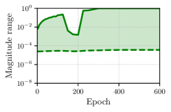
Independent loss

Figure 11: Joint vs. independent optimization. The effect of learning magnitude ranges by jointly optimizing the loss terms $\mathcal{L}_{\text{ra}}$ and $\mathcal{L}_{\text{task}}$ (top row) compared to only optimizing $\mathcal{L}_{\text{ra}}$ (bottom row) is shown for ResNet-50 on the ImageNet dataset. Training ResNet-50 with the joint loss leads to smaller magnitudes of noise, and improves validation accuracy by approximately $1\%$ on the ImageNet dataset.

Effect of joint vs. independent optimization

An expected behavior for learning model-specific augmentation policy using RangeAugment is that task-specific loss $\mathcal{L}_{\text{task}}$ in Eq. 2 should contribute towards policy learning. To validate it, ResNet-50 is trained independently as well as jointly on the ImageNet dataset. We found that the top-1 accuracy of ResNet-50 dropped by about 1% when it is trained independently. This is likely because independent training allowed RangeAugment to produce augmented images with more additive Gaussian noise (Fig. 11), resulting in performance drop. This concurs with our observations in Section 4, especially Figs. 5 and 6, where we found that sampling augmented images from wider magnitude range for additive Gaussian noise operation dropped ResNet-50’s performance on the ImageNet dataset. A plausible explanation is that PSNR is more sensitive to noise operation (Hore & Ziou, 2010), allowing RangeAugment to learn wider magnitude ranges for noise operation when trained independently as compared to joint training. Overall, these results suggest that joint training helps in learning model-specific policy.

Appendix B Visualization of augmented samples

Fig. 12 visualizes augmented samples produced by RangeAugment at different stages of training ResNet-50 with curriculum. We can see that the range of magnitudes (Fig. 12(a)) and diversity of augmented samples (Fig. 12(b)) increases as training progresses.

$\Delta$	Brightness	Contrast	Noise
$40\rightarrow 5$

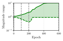
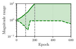
(a)

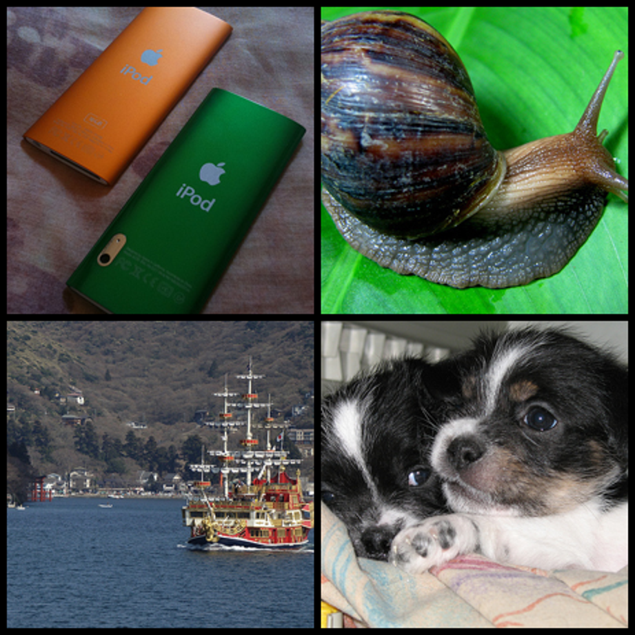
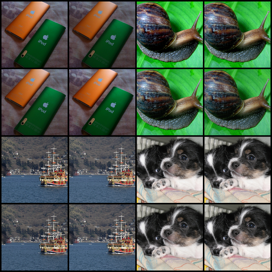
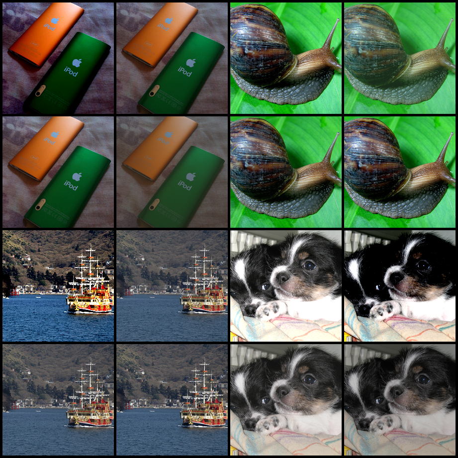
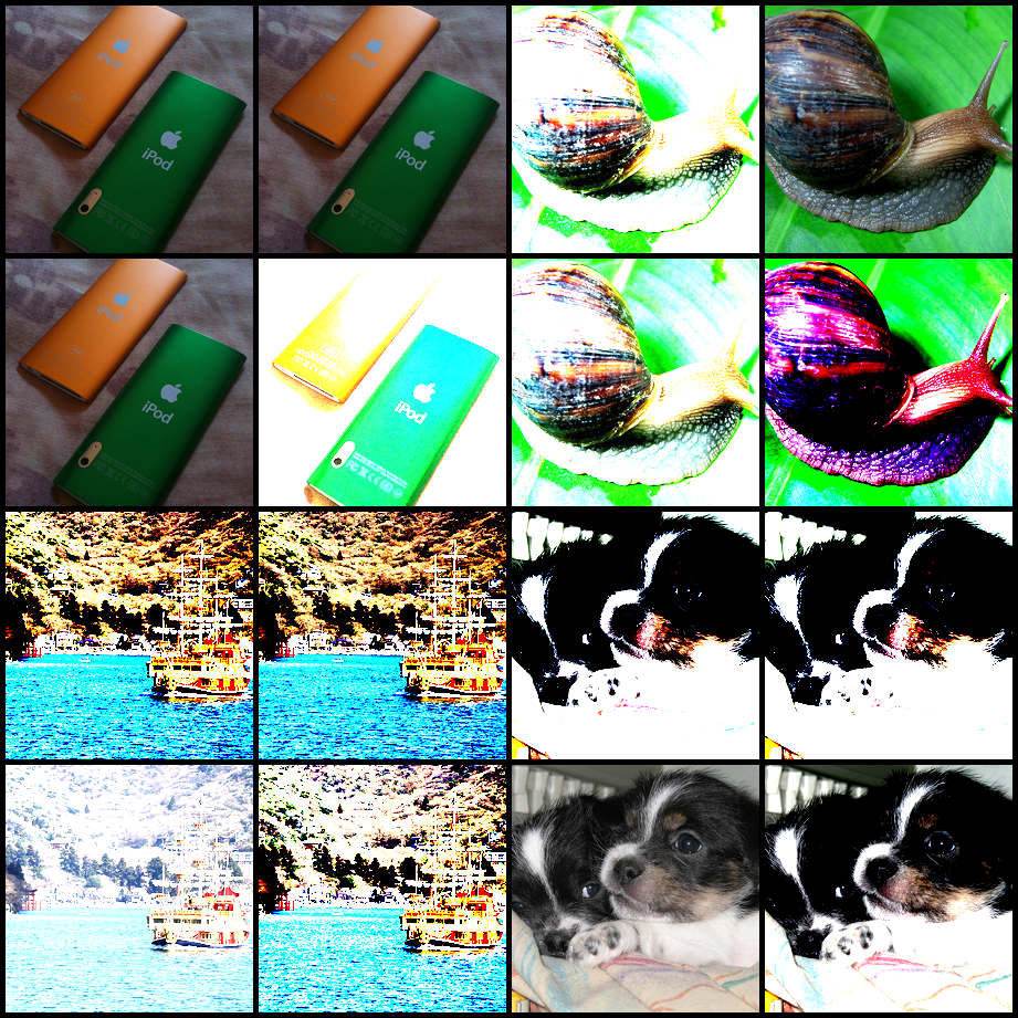
Input images	Epoch 1	Epoch 100	Epoch 200	Epoch 600

(b)

Figure 12: Visualization of augmented samples. (a) Learned magnitude ranges of different augmentations when ResNet-50 is trained jointly with RangeAugment using a cosine curriculum. (b) Four image samples visualized at different epoch intervals. For illustration purposes, we visualize four random augmented samples produced by RangeAugment for each image.

Appendix C Learned Magnitude Ranges for CLIP with RangeAugment

Fig. 13 shows the learned magnitude ranges of different augmentation operations for training the CLIP model with RangeAugment. Unlike image classification (Section 4) and semantic segmentation (Section 5.1) results, the CLIP model uses little augmentation. This is expected because image-text pair datasets are orders of magnitude larger than classification and segmentation datasets.

Brightness	Contrast	Noise

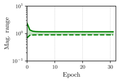
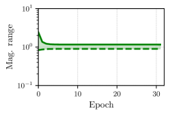
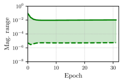
Figure 13: Learned magnitude ranges of different augmentations for CLIP with ViT-B/16. Target PSNR $\Delta$ is annealed from 40 to 20.

Appendix D Training Details

D.1 Training Hyper-parameters

Table 7 summarizes training recipe used for training different models across different tasks.

		Non-mobile models					Mobile models
	ResNet-50	ResNet-101	EfficientNet	SwinTransformer		MobileViT	MobileNetv1	MobileNetv2	MobileNetv3
Epochs	600	600	400	300		300	300	300	300
Batch size	1024	1024	2048	1024		1024	512	1024	2048
Data sampler	MSc-VBS	MSc-VBS	MSc-VBS	SSc-FBS		MSc-VBS	MSc-VBS	MSc-VBS	MSc-VBS
Max. LR	$0.4$	$0.4$	$0.8$	$10^{-3}$		$2\times 10^{-3}$	$0.4$	$0.4$	$0.8$
Min. LR	$2\times 10^{-4}$	$2\times 10^{-4}$	$4\times 10^{-4}$	$10^{-5}$		$2\times 10^{-4}$	$2\times 10^{-4}$	$2\times 10^{-4}$	$4\times 10^{-4}$
Warmup init. LR	0.05	0.05	0.1	$10^{-6}$		$2\times 10^{-4}$	$0.05$	$0.05$	$0.1$
Warmup epochs	5	5	5	20		16	3	6	5
LR Annealing	cosine	cosine	cosine	cosine		cosine	cosine	cosine	cosine
Weight decay	$4\times 10^{-5}$	$4\times 10^{-5}$	$4\times 10^{-5}$	$5\times 10^{-2}$		0.01	$4\times 10^{-5}$	$4\times 10^{-5}$	$4\times 10^{-5}$
Optimizer	SGD	SGD	SGD	AdamW		AdamW	SGD	SGD	SGD
Momentum	0.9	0.9	0.9	✗		✗	0.9	0.9	0.9
Label smoothing $\epsilon$	0.1	0.1	0.1	0.1		0.1	0.1	0.1	0.1
Stoch. Depth	✗	✗	✗	0.3		✗	✗	✗	✗
Grad. clipping	✗	✗	✗	5.0		✗	✗	✗	✗
# parameters	25.6 M	44.5 M	12.3 M	49.6 M		5.6 M	4.2 M	3.5 M	5.4 M
# FLOPs	4.0 G	7.7 G	1.9 G	8.8 G		2.0 G	579 M	314 M	220 M

(a) Image classification on ImageNet

Hyperparameter	ADE20k	PASCAL VOC
Epochs	50	50
Batch size	16	128
Data sampler	SSc-FBS	SSc-FBS
Max. LR	$0.02$	0.02
Min. LR	$10^{-4}$	$10^{-4}$
LR Annealing	cosine	cosine
Weight decay	$10^{-4}$	$10^{-4}$
Optimizer	SGD	SGD

(b) Semantic segmentation with DeepLabv3

Hyperparameter	COCO
Epochs	100
Batch size	32
Data sampler	MSc-VBS
Warm-up iterations	500
Warm-up init. LR	0.001
LR	0.1
LR annealing	Multi-step
LR annealing factor	0.1
Annealing epochs	[60, 84 ]
Weight decay	0.2
Optimizer	SGD

(c) Object detection with Mask R-CNN

Hyperparameter	CLIP-VIT-B/16	CLIP-VIT-B/16	CLIP-VIT-H/16
# image-text pairs	302M	1.1B	1.1B
Epochs/iterations	32	150k	120k
Batch size	32k	65k	132k
Data sampler	MSc-VBS	MSc-VBS	MSc-VBS
Warm-up iterations	2000	1000	1000
Warm-up init. LR	$10^{-6}$	$10^{-6}$	$10^{-6}$
Max. LR	$5^{-4}$	$5^{-4}$	$5^{-4}$
Min. LR	$10^{-6}$	$10^{-6}$	$10^{-6}$
LR Annealing	cosine	cosine	cosine
Weight decay	0.2	0.2	0.2
Optimizer	AdamW	AdamW	AdamW

(d) CLIP models

Table 7: Hyper-parameters used for training models on different tasks. Here, SSc-FBS and MSc-VBS refers to single-scale fixed batch size and multi-scale variable batch size data samplers respectively (Mehta et al., 2022). We found that the performance of CLIP models with smaller (32k) and larger (65k or 132k) batch sizes is similar. We used large batch sizes for faster training.

D.2 Bounds for Augmentation operations

Table 8 shows the clipping bounds that RangeAugment uses to prevent training instability.

Operation	Clipping bounds in RangeAugment		Magnitude range in AutoAugment
	Min.	Max.	(reference)
Brightness	0.1	10.0	[0.1 - 1.9]
Contrast	0.1	10.0	[0.1 - 1.9]
Noise (std. dev)	0	1.0	–

Table 8: Clipping bounds used in RangeAugment for preventing training instability. The range of magnitudes for augmentation operations in AutoAugment is also given as a reference.

References

- Asiedu et al. (2022) Emmanuel Brempong Asiedu, Simon Kornblith, Ting Chen, Niki Parmar, Matthias Minderer, and Mohammad Norouzi. Decoder denoising pretraining for semantic segmentation. arXiv preprint arXiv:2205.11423, 2022.
- Bengio et al. (2009) Yoshua Bengio, Jérôme Louradour, Ronan Collobert, and Jason Weston. Curriculum learning. In Proceedings of the 26th annual international conference on machine learning, pp. 41–48, 2009.
- Chen et al. (2017) Liang-Chieh Chen, George Papandreou, Florian Schroff, and Hartwig Adam. Rethinking atrous convolution for semantic image segmentation. arXiv preprint arXiv:1706.05587, 2017.
- Chen et al. (2018) Liang-Chieh Chen, Yukun Zhu, George Papandreou, Florian Schroff, and Hartwig Adam. Encoder-decoder with atrous separable convolution for semantic image segmentation. In Proceedings of the European conference on computer vision (ECCV), pp. 801–818, 2018.
- Cubuk et al. (2019) Ekin D Cubuk, Barret Zoph, Dandelion Mane, Vijay Vasudevan, and Quoc V Le. Autoaugment: Learning augmentation strategies from data. In Proceedings of the IEEE/CVF Conference on Computer Vision and Pattern Recognition, pp. 113–123, 2019.
- Cubuk et al. (2020) Ekin D Cubuk, Barret Zoph, Jonathon Shlens, and Quoc V Le. Randaugment: Practical automated data augmentation with a reduced search space. In Proceedings of the IEEE/CVF conference on computer vision and pattern recognition workshops, pp. 702–703, 2020.
- Deng et al. (2009) Jia Deng, Wei Dong, Richard Socher, Li-Jia Li, Kai Li, and Li Fei-Fei. Imagenet: A large-scale hierarchical image database. In 2009 IEEE conference on computer vision and pattern recognition, pp. 248–255. Ieee, 2009.
- Dollár et al. (2021) Piotr Dollár, Mannat Singh, and Ross Girshick. Fast and accurate model scaling. In Proceedings of the IEEE/CVF Conference on Computer Vision and Pattern Recognition, pp. 924–932, 2021.
- Dosovitskiy et al. (2020) Alexey Dosovitskiy, Lucas Beyer, Alexander Kolesnikov, Dirk Weissenborn, Xiaohua Zhai, Thomas Unterthiner, Mostafa Dehghani, Matthias Minderer, Georg Heigold, Sylvain Gelly, et al. An image is worth 16x16 words: Transformers for image recognition at scale. arXiv preprint arXiv:2010.11929, 2020.
- Everingham et al. (2010) Mark Everingham, Luc Van Gool, Christopher KI Williams, John Winn, and Andrew Zisserman. The pascal visual object classes (voc) challenge. International journal of computer vision, 88(2):303–338, 2010.
- Hataya et al. (2020) Ryuichiro Hataya, Jan Zdenek, Kazuki Yoshizoe, and Hideki Nakayama. Faster autoaugment: Learning augmentation strategies using backpropagation. In European Conference on Computer Vision, pp. 1–16. Springer, 2020.
- He et al. (2016) Kaiming He, Xiangyu Zhang, Shaoqing Ren, and Jian Sun. Deep residual learning for image recognition. In Proceedings of the IEEE conference on computer vision and pattern recognition, pp. 770–778, 2016.
- He et al. (2017) Kaiming He, Georgia Gkioxari, Piotr Dollár, and Ross Girshick. Mask r-cnn. In Proceedings of the IEEE international conference on computer vision, pp. 2961–2969, 2017.
- Ho et al. (2019) Daniel Ho, Eric Liang, Xi Chen, Ion Stoica, and Pieter Abbeel. Population based augmentation: Efficient learning of augmentation policy schedules. In International Conference on Machine Learning, pp. 2731–2741. PMLR, 2019.
- Hore & Ziou (2010) Alain Hore and Djemel Ziou. Image quality metrics: Psnr vs. ssim. In 2010 20th international conference on pattern recognition, pp. 2366–2369. IEEE, 2010.
- Howard et al. (2019) Andrew Howard, Mark Sandler, Grace Chu, Liang-Chieh Chen, Bo Chen, Mingxing Tan, Weijun Wang, Yukun Zhu, Ruoming Pang, Vijay Vasudevan, et al. Searching for mobilenetv3. In Proceedings of the IEEE/CVF international conference on computer vision, pp. 1314–1324, 2019.
- Howard et al. (2017) Andrew G Howard, Menglong Zhu, Bo Chen, Dmitry Kalenichenko, Weijun Wang, Tobias Weyand, Marco Andreetto, and Hartwig Adam. Mobilenets: Efficient convolutional neural networks for mobile vision applications. arXiv preprint arXiv:1704.04861, 2017.
- Ilharco et al. (2021) Gabriel Ilharco, Mitchell Wortsman, Ross Wightman, Cade Gordon, Nicholas Carlini, Rohan Taori, Achal Dave, Vaishaal Shankar, Hongseok Namkoong, John Miller, Hannaneh Hajishirzi, Ali Farhadi, and Ludwig Schmidt. Openclip, July 2021. URL https://doi.org/10.5281/zenodo.5143773.
- Jiang et al. (2020) Yiding Jiang, Behnam Neyshabur, Hossein Mobahi, Dilip Krishnan, and Samy Bengio. Fantastic generalization measures and where to find them. In International Conference on Learning Representations, 2020.
- Kingma & Welling (2013) Diederik P Kingma and Max Welling. Auto-encoding variational bayes. arXiv preprint arXiv:1312.6114, 2013.
- Krizhevsky et al. (2012) Alex Krizhevsky, Ilya Sutskever, and Geoffrey E Hinton. Imagenet classification with deep convolutional neural networks. In F. Pereira, C.J. Burges, L. Bottou, and K.Q. Weinberger (eds.), Advances in Neural Information Processing Systems, volume 25. Curran Associates, Inc., 2012.
- LeCun et al. (1998) Yann LeCun, Léon Bottou, Yoshua Bengio, and Patrick Haffner. Gradient-based learning applied to document recognition. Proceedings of the IEEE, 86(11):2278–2324, 1998.
- Lemley et al. (2017) Joseph Lemley, Shabab Bazrafkan, and Peter Corcoran. Smart augmentation learning an optimal data augmentation strategy. Ieee Access, 5:5858–5869, 2017.
- Li et al. (2020) Yonggang Li, Guosheng Hu, Yongtao Wang, Timothy Hospedales, Neil M Robertson, and Yongxin Yang. Differentiable automatic data augmentation. In European Conference on Computer Vision, pp. 580–595. Springer, 2020.
- Lim et al. (2019) Sungbin Lim, Ildoo Kim, Taesup Kim, Chiheon Kim, and Sungwoong Kim. Fast autoaugment. Advances in Neural Information Processing Systems, 32, 2019.
- Lin et al. (2014) Tsung-Yi Lin, Michael Maire, Serge Belongie, James Hays, Pietro Perona, Deva Ramanan, Piotr Dollár, and C Lawrence Zitnick. Microsoft coco: Common objects in context. In European conference on computer vision, pp. 740–755. Springer, 2014.
- LingChen et al. (2020) Tom Ching LingChen, Ava Khonsari, Amirreza Lashkari, Mina Rafi Nazari, Jaspreet Singh Sambee, and Mario A Nascimento. Uniformaugment: A search-free probabilistic data augmentation approach. arXiv preprint arXiv:2003.14348, 2020.
- Liu et al. (2021a) Aoming Liu, Zehao Huang, Zhiwu Huang, and Naiyan Wang. Direct differentiable augmentation search. In Proceedings of the IEEE/CVF International Conference on Computer Vision, pp. 12219–12228, 2021a.
- Liu et al. (2021b) Ze Liu, Yutong Lin, Yue Cao, Han Hu, Yixuan Wei, Zheng Zhang, Stephen Lin, and Baining Guo. Swin transformer: Hierarchical vision transformer using shifted windows. In Proceedings of the IEEE/CVF International Conference on Computer Vision, pp. 10012–10022, 2021b.
- Liu et al. (2022) Zhuang Liu, Hanzi Mao, Chao-Yuan Wu, Christoph Feichtenhofer, Trevor Darrell, and Saining Xie. A convnet for the 2020s. Proceedings of the IEEE/CVF Conference on Computer Vision and Pattern Recognition (CVPR), 2022.
- Mehta & Rastegari (2021) Sachin Mehta and Mohammad Rastegari. Mobilevit: light-weight, general-purpose, and mobile-friendly vision transformer. arXiv preprint arXiv:2110.02178, 2021.
- Mehta et al. (2022) Sachin Mehta, Farzad Abdolhosseini, and Mohammad Rastegari. Cvnets: High performance library for computer vision. arXiv preprint arXiv:2206.02002, 2022.
- MMSegmentation (2020) Contributors MMSegmentation. MMSegmentation: Openmmlab semantic segmentation toolbox and benchmark. https://github.com/open-mmlab/mmsegmentation, 2020.
- Müller & Hutter (2021) Samuel G Müller and Frank Hutter. Trivialaugment: Tuning-free yet state-of-the-art data augmentation. In Proceedings of the IEEE/CVF International Conference on Computer Vision, pp. 774–782, 2021.
- Perez & Wang (2017) Luis Perez and Jason Wang. The effectiveness of data augmentation in image classification using deep learning. arXiv preprint arXiv:1712.04621, 2017.
- Radford et al. (2021) Alec Radford, Jong Wook Kim, Chris Hallacy, Aditya Ramesh, Gabriel Goh, Sandhini Agarwal, Girish Sastry, Amanda Askell, Pamela Mishkin, Jack Clark, et al. Learning transferable visual models from natural language supervision. In International Conference on Machine Learning, pp. 8748–8763. PMLR, 2021.
- Radosavovic et al. (2020) Ilija Radosavovic, Raj Prateek Kosaraju, Ross Girshick, Kaiming He, and Piotr Dollár. Designing network design spaces. In Proceedings of the IEEE/CVF conference on computer vision and pattern recognition, pp. 10428–10436, 2020.
- Ratner et al. (2017) Alexander J Ratner, Henry Ehrenberg, Zeshan Hussain, Jared Dunnmon, and Christopher Ré. Learning to compose domain-specific transformations for data augmentation. Advances in neural information processing systems, 30, 2017.
- Sandler et al. (2018) Mark Sandler, Andrew Howard, Menglong Zhu, Andrey Zhmoginov, and Liang-Chieh Chen. Mobilenetv2: Inverted residuals and linear bottlenecks. In Proceedings of the IEEE conference on computer vision and pattern recognition, pp. 4510–4520, 2018.
- Steiner et al. (2021) Andreas Steiner, Alexander Kolesnikov, Xiaohua Zhai, Ross Wightman, Jakob Uszkoreit, and Lucas Beyer. How to train your vit? data, augmentation, and regularization in vision transformers. arXiv preprint arXiv:2106.10270, 2021.
- Szegedy et al. (2015) Christian Szegedy, Wei Liu, Yangqing Jia, Pierre Sermanet, Scott Reed, Dragomir Anguelov, Dumitru Erhan, Vincent Vanhoucke, and Andrew Rabinovich. Going deeper with convolutions. In Proceedings of the IEEE conference on computer vision and pattern recognition, pp. 1–9, 2015.
- Tan & Le (2019) Mingxing Tan and Quoc Le. Efficientnet: Rethinking model scaling for convolutional neural networks. In International conference on machine learning, pp. 6105–6114. PMLR, 2019.
- Tan & Le (2021) Mingxing Tan and Quoc Le. Efficientnetv2: Smaller models and faster training. In International Conference on Machine Learning, pp. 10096–10106. PMLR, 2021.
- Touvron et al. (2019) Hugo Touvron, Andrea Vedaldi, Matthijs Douze, and Hervé Jégou. Fixing the train-test resolution discrepancy. Advances in neural information processing systems, 32, 2019.
- Touvron et al. (2021) Hugo Touvron, Matthieu Cord, Matthijs Douze, Francisco Massa, Alexandre Sablayrolles, and Hervé Jégou. Training data-efficient image transformers & distillation through attention. In International Conference on Machine Learning, pp. 10347–10357. PMLR, 2021.
- Wightman et al. (2021) Ross Wightman, Hugo Touvron, and Herve Jegou. Resnet strikes back: An improved training procedure in timm. In NeurIPS 2021 Workshop on ImageNet: Past, Present, and Future, 2021. URL https://openreview.net/forum?id=NG6MJnVl6M5.
- Wu et al. (2019) Yuxin Wu, Alexander Kirillov, Francisco Massa, Wan-Yen Lo, and Ross Girshick. Detectron2. https://github.com/facebookresearch/detectron2, 2019.
- Xiao et al. (2018) Tete Xiao, Yingcheng Liu, Bolei Zhou, Yuning Jiang, and Jian Sun. Unified perceptual parsing for scene understanding. In Proceedings of the European conference on computer vision (ECCV), pp. 418–434, 2018.
- Xie et al. (2021) Enze Xie, Wenhai Wang, Zhiding Yu, Anima Anandkumar, Jose M Alvarez, and Ping Luo. Segformer: Simple and efficient design for semantic segmentation with transformers. Advances in Neural Information Processing Systems, 34:12077–12090, 2021.
- Yun et al. (2019) Sangdoo Yun, Dongyoon Han, Seong Joon Oh, Sanghyuk Chun, Junsuk Choe, and Youngjoon Yoo. Cutmix: Regularization strategy to train strong classifiers with localizable features. In Proceedings of the IEEE/CVF international conference on computer vision, pp. 6023–6032, 2019.
- Zhai et al. (2022) Xiaohua Zhai, Alexander Kolesnikov, Neil Houlsby, and Lucas Beyer. Scaling vision transformers. In Proceedings of the IEEE/CVF Conference on Computer Vision and Pattern Recognition, pp. 12104–12113, 2022.
- Zhang et al. (2018) Hongyi Zhang, Moustapha Cisse, Yann N. Dauphin, and David Lopez-Paz. mixup: Beyond empirical risk minimization. In International Conference on Learning Representations, 2018. URL https://openreview.net/forum?id=r1Ddp1-Rb.
- Zhao et al. (2017) Hengshuang Zhao, Jianping Shi, Xiaojuan Qi, Xiaogang Wang, and Jiaya Jia. Pyramid scene parsing network. In Proceedings of the IEEE conference on computer vision and pattern recognition, pp. 2881–2890, 2017.
- Zheng et al. (2021) Yu Zheng, Zhi Zhang, Shen Yan, and Mi Zhang. Deep autoaugment. In International Conference on Learning Representations, 2021.
- Zheng et al. (2022) Yu Zheng, Zhi Zhang, Shen Yan, and Mi Zhang. Deep autoaugment. In International Conference on Learning Representations, 2022. URL https://openreview.net/forum?id=St-53J9ZARf.
- Zhou et al. (2017) Bolei Zhou, Hang Zhao, Xavier Puig, Sanja Fidler, Adela Barriuso, and Antonio Torralba. Scene parsing through ade20k dataset. In Proceedings of the IEEE conference on computer vision and pattern recognition, pp. 633–641, 2017.
- Zoph & Le (2017) Barret Zoph and Quoc Le. Neural architecture search with reinforcement learning. In International Conference on Learning Representations, 2017. URL https://openreview.net/forum?id=r1Ue8Hcxg.