$\mbox{}^{\diamond}$ This author’s work was supported in part by the NSERC Discovery Grants RGPIN-2020-06022 and DGECR-2020-00356.

$\mbox{}^{\dagger}$ Dept. of Computer Science, University of Toronto, Toronto, ON M5S 2E4
$\mbox{}^{\ddagger}$ Dept. of Math. and Computer Science, University of Toronto, Toronto, ON M5S 2E4

$\mbox{}^{\star}$ Corresponding author

1 Introduction

Function approximation has been a central topic in numerical analysis since its inception. One of the most effective methods for approximating a function $F:[-1,1]\to\mathbbm{R}$ is the use of an interpolating polynomial $P_{N}$ of degree $N$ which satisfies $P_{N}(x_{j})=F(x_{j})$ for a set of $(N+1)$ collocation points $\{x_{j}\}_{j=0,1,\dots,N}$. In practice, the collocation points are typically chosen to be the Chebyshev points, and the resulting interpolating polynomial, known as the Chebyshev interpolant, is a nearly optimal approximation to $F$ in the space of polynomials of degree at most $N$ [27]. A common basis for representing the interpolating polynomial $P_{N}$ is the Lagrange polynomial basis, and the evaluation of $P_{N}$ in this basis can be done stably using the Barycentric interpolation formula [8, 19]. Some other commonly used bases are Newton polynomials, Chebyshev polynomials, and Legendre polynomials. Alternatively, the monomial basis can be used to represent $P_{N}$, such that $P_{N}(x)=\sum_{k=0}^{N}a_{k}x^{k}$ for some coefficients $\{a_{k}\}_{k=0,1,\dots,N}$. The computation of the monomial coefficient vector $a:=(a_{0},a_{1},\dots,a_{N})^{T}\in\mathbbm{R}^{N+1}$ of the interpolating polynomial $P_{N}$ requires the solution to a linear system $Va=f$, where

$$V:=\begin{pmatrix}1&x_{0}&x_{0}^{2}&\cdots&x_{0}^{N}\\ 1&x_{1}&x_{1}^{2}&\cdots&x_{1}^{N}\\ \vdots&\vdots&\vdots&\ddots&\vdots\\ 1&x_{N}&x_{N}^{2}&\cdots&x_{N}^{N}\\ \end{pmatrix}\in\mathbbm{R}^{(N+1)\times(N+1)}$$ (1)

is a Vandermonde matrix, and $f:=\bigl{(}F(x_{0}),F(x_{1}),\dots,F(x_{N})\bigr{)}^{T}\in\mathbbm{R}^{N+1}$ is a vector of the function values of $F$ at the $(N+1)$ collocation points on the interval $[-1,1]$. It is well-known that, given any set of real collocation points, the condition number of a Vandermonde matrix grows at least exponentially as $N$ increases [7]. It follows that the numerical solution to this linear system is highly inaccurate when $N$ is not small, and, as a result, this algorithm for constructing $P_{N}$ is often considered to be unstable. But, is this really the case? Let $\{x_{j}\}_{j=0,1,\dots,N}$ be the set of $(N+1)$ Chebyshev points on the interval $[-1,1]$, and consider the case where $F(x)=\cos(2x+1)$. We solve the resulting Vandermonde system using LU factorization with partial pivoting. In Figure 1(a), we present a comparison between the approximation error of the computed monomial expansion (labeled as “Monomial”) and the approximation error of the Chebyshev interpolant evaluated using the Barycentric interpolation formula (labeled as “Lagrange”). One can observe that the computed monomial expansion is, surprisingly, as accurate as the Chebyshev interpolant evaluated using the Barycentric interpolation formula (which is accurate up to machine precision), despite the huge condition number of the Vandermonde matrix reported in Figure 1(b).

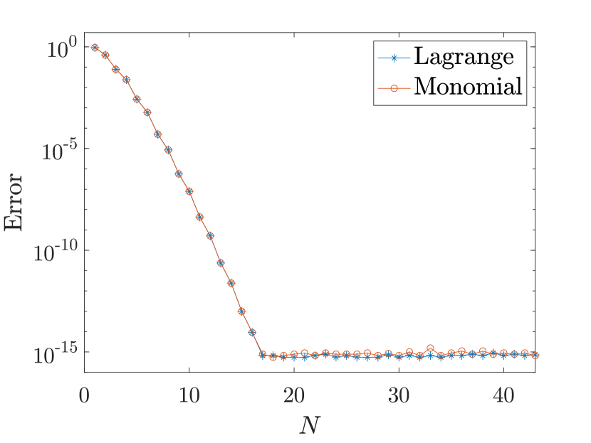
(a) $\cos(2x+1)$

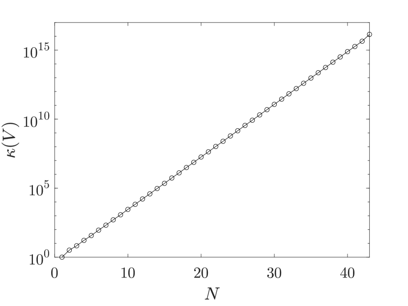
(b) Condition number

Figure 1: Polynomial interpolation of $\cos(2x+1)$ in the monomial basis. The $x$-axis label $N$ denotes the order of approximation. The $y$-axis label “Error” denotes the $L^{\infty}$ approximation error over $[-1,1]$, which is estimated by comparing the approximated function values at $10000$ equidistant points over $[-1,1]$ with the true function values.

What happens when the function $F$ becomes more complicated? In Figure 2, we compare the accuracy of the two approximations when $F(x)=\cos(8x+1)$ and when $F(x)=\cos(12x+1)$. Initially, the computed monomial expansion is as accurate as the Chebyshev interpolant evaluated using the Barycentric interpolation formula. However, the convergence of polynomial interpolation in the monomial basis stagnates after reaching a certain error threshold. Furthermore, it appears that, the more complicated a function is, the larger that error threshold becomes. But what does it mean for a function to be complicated in this context? Consider the case where the function requires an even higher-order Chebyshev interpolant in order to be approximated to machine precision. In Figure 3, we compare the accuracy of the two approximations when $F(x)=\frac{1}{x-\sqrt{2}}$ and when $F(x)=\frac{1}{x-0.5i}$. These two functions each have a singularity in a neighborhood of the interval $[-1,1]$, and Chebyshev interpolants of degree $\geq 40$ are required to approximate them to machine precision. Yet, no stagnation of convergence is observed. In Figure 4, we consider the case where $F$ is a non-smooth function, and we find that the accuracy of the two approximations is, again, the same. Based on all of the previous examples, we conclude that polynomial interpolation in the monomial basis is not as unstable as it appears, and has some subtleties lurking around the corner that are worth further investigation.

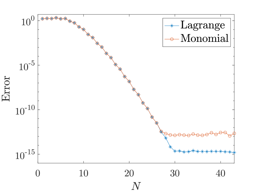
(a) $\cos(8x+1)$

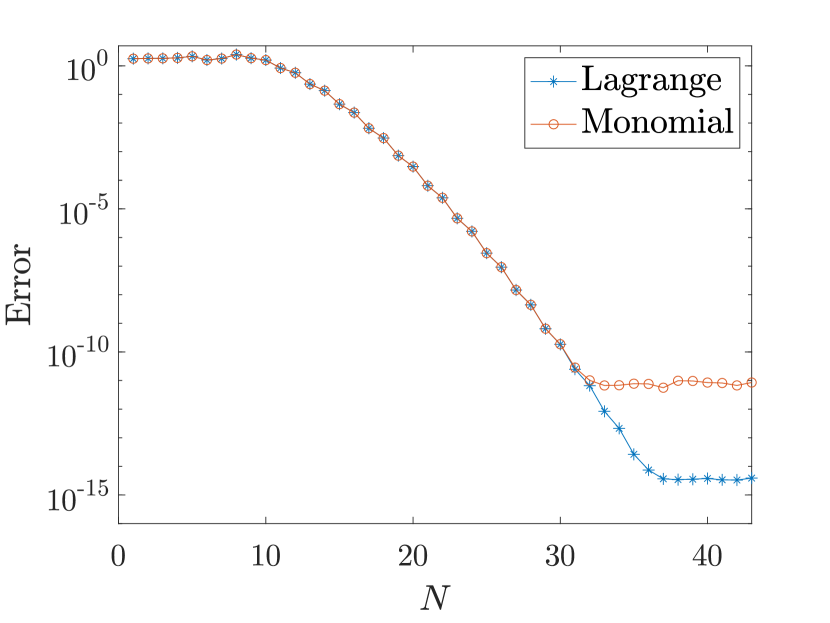
(b) $\cos(12x+1)$

Figure 2: Polynomial interpolation of more complicated functions in the monomial basis.

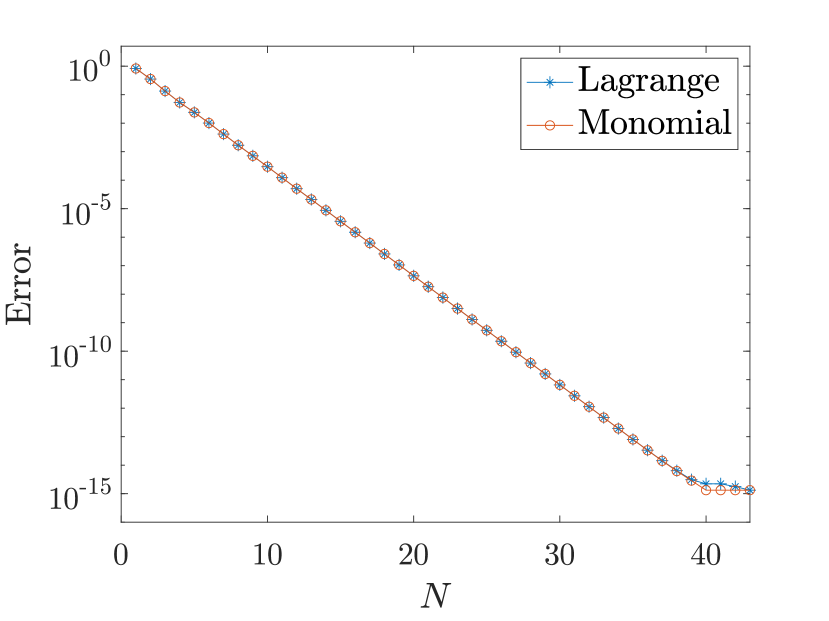
(a) $\frac{1}{x-\sqrt{2}}$

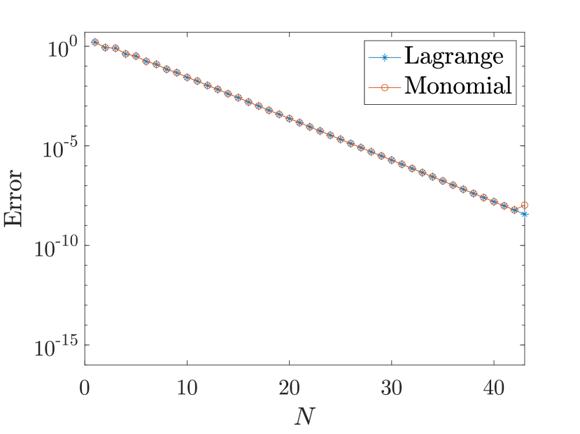
(b) $\frac{1}{x-0.5i}$

Figure 3: Polynomial interpolation of functions with a singularity near the interval $[-1,1]$ in the monomial basis.

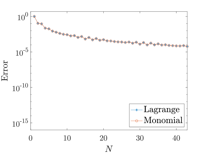
(a) ${\lvert x+0.1\rvert}^{2.5}$

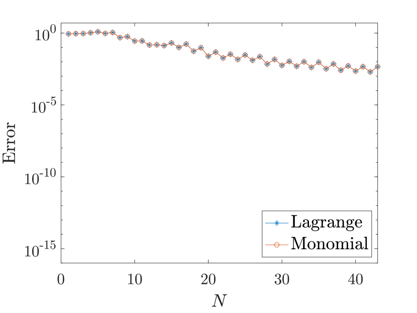
(b) ${\lvert\sin(5x)\rvert}^{3}$

Figure 4: Polynomial interpolation of non-smooth functions in the monomial basis.

These seemingly mysterious experiments can be explained partially from the point of view of backward error analysis. Indeed, the forward error ${\lVert a-\widehat{a}\rVert}_{2}$ of the numerical solution $\widehat{a}$ to the Vandermonde system $Va=f$ can be huge, but it is the backward error, i.e., ${\lVert V\widehat{a}-f\rVert}_{2}$, that matters for the accuracy of the approximation. This is because a small backward error implies that the difference between the computed monomial expansion, which we denote by $\widehat{P}_{N}$, and the exact interpolating polynomial, $P_{N}$, is a polynomial that approximately vanishes at all of the collocation points. When the Lebesgue constant associated with the collocation points is small (which is the case for the Chebyshev points), the polynomial $P_{N}-\widehat{P}_{N}$ is bounded uniformly by the backward error times a small constant. As a result, we bound the monomial approximation error ${\lVert F-\widehat{P}_{N}\rVert}_{L^{\infty}([-1,1])}$ by the following inequality:

$${\lVert F-\widehat{P}_{N}\rVert}_{L^{\infty}([-1,1])}\leq{\lVert F-P_{N}\rVert}_{L^{\infty}([-1,1])}+{\lVert P_{N}-\widehat{P}_{N}\rVert}_{L^{\infty}([-1,1])}.$$ (2)

We refer to the first and the second terms on the right-hand side of (2) as the polynomial interpolation error and the backward error, respectively. When the backward error is smaller than the polynomial interpolation error, the monomial approximation error is dominated by the polynomial interpolation error, and the use of a monomial basis does not incur any additional loss of accuracy. Once the polynomial interpolation error becomes smaller than the backward error, the convergence of the approximation stagnates. For example, in Figure 3(a), we verify numerically that the backward error is around the size of machine epsilon for all $N\leq 43$, so stagnation is not observed, and polynomial interpolation in the monomial basis is as accurate as polynomial interpolation in the Lagrange basis, evaluated by the Barycentric interpolation formula. On the other hand, in Figure 2(a), the backward error is around the size of $10^{-13}$ for $N\geq 20$, which leads to stagnation once the polynomial interpolation error is less than $10^{-13}$.

The explanation above brings up a new question: when will the backward error be small? When a backward stable linear system solver (e.g., LU factorization with partial pivoting) is used to solve the Vandermonde system $Va=f$, it is guaranteed that the numerical solution $\widehat{a}$ is the exact solution to the linear system

$$(V+\delta V)\widehat{a}=f,$$ (3)

for a matrix $\delta V\in\mathbbm{R}^{(N+1)\times(N+1)}$ that satisfies ${\lVert\delta V\rVert}_{2}\leq u\cdot\gamma$, where $u$ denotes machine epsilon and $\gamma=\mathcal{O}({\lVert V\rVert}_{2})$. It follows that the backward error, ${\lVert V\widehat{a}-f\rVert}_{2}$, of the numerical solution is bounded by $u\cdot\gamma{\lVert\widehat{a}\rVert}_{2}$. We note that $\gamma$ is typically small, so the backward error is essentially determined by the norm of the computed monomial coefficient vector. In fact, so long as $\kappa(V)\lesssim\frac{1}{u}$, one can show that the norm of the monomial coefficient vector computed by a backward stable solver is around the same size as the norm of the exact monomial coefficient vector of the interpolating polynomial. Therefore, in this case, the monomial approximation error can be quantified a priori using information about the interpolating polynomial, which implies that a theory of polynomial interpolation in the monomial basis can be developed.

The rest of the paper is organized as follows. In Section 2, we analyze polynomial interpolation in the monomial basis over a smooth simple arc in the complex plane, with the interval as a special case, along with a number of numerical experiments. Our analysis shows that the monomial basis is similar to a well-conditioned polynomial basis for interpolation, provided that the condition number of the Vandermonde matrix is smaller than the reciprocal of machine epsilon. In Section 3, we present applications where the use of a monomial basis for interpolation offers a substantial advantage over other bases. In Section 4, we review related work, and discuss the generalization of our theory to higher dimensions.

2 Polynomial interpolation in the monomial basis

Let $\Gamma\subset\mathbbm{C}$ be a smooth simple arc, and let $F:\Gamma\to\mathbbm{C}$ be an arbitrary function. The $N$th degree interpolating polynomial, denoted by $P_{N}$, of the function $F$ for a given set of $(N+1)$ distinct collocation points $Z:=\{z_{j}\}_{j=0,1,\dots,N}\subset\Gamma$ can be expressed as $P_{N}(z)=\sum_{k=0}^{N}a_{k}z^{k}$, where the monomial coefficient vector $(a_{0},a_{1},\dots,a_{N})^{T}$ is the solution to the Vandermonde system

$$\begin{pmatrix}1&z_{0}&z_{0}^{2}&\cdots&z_{0}^{N}\\ 1&z_{1}&z_{1}^{2}&\cdots&z_{1}^{N}\\ \vdots&\vdots&\vdots&\ddots&\vdots\\ 1&z_{N}&z_{N}^{2}&\cdots&z_{N}^{N}\\ \end{pmatrix}\begin{pmatrix}a_{0}\\ a_{1}\\ \vdots\\ a_{N}\\ \end{pmatrix}=\begin{pmatrix}F(z_{0})\\ F(z_{1})\\ \vdots\\ F(z_{N})\\ \end{pmatrix}.$$ (4)

For ease of notation, we denote the Vandermonde matrix by $V^{(N)}$, the monomial coefficient vector by $a^{(N)}$, and the corresponding right-hand side vector by $f^{(N)}$.

In order to study the size of the residual of the numerical solution to the Vandermonde system, we require the following lemma, which provides a bound for the 2-norm of the solution to a perturbed linear system.

Lemma 2.1.

Let $N$ be a positive integer. Suppose that $A\in\mathbbm{C}^{N\times N}$ is invertible, $b\in\mathbbm{C}^{N}$, and that $x\in\mathbbm{C}^{N}$ satisfies $Ax=b$. Suppose further that $\widehat{x}\in\mathbbm{C}^{N}$ satisfies $(A+\delta A)\widehat{x}=b$ for some $\delta A\in\mathbbm{C}^{N\times N}$. If there exists an $\alpha>1$ such that

$${\lVert A^{-1}\rVert}_{2}\leq\frac{1}{\alpha\cdot{\lVert\delta A\rVert}_{2}},$$ (5)

then the matrix $A+\delta A$ is invertible, and $\widehat{x}$ satisfies

$$\frac{\alpha}{\alpha+1}{\lVert x\rVert}_{2}\leq{\lVert\widehat{x}\rVert}_{2}\leq\frac{\alpha}{\alpha-1}{\lVert x\rVert}_{2}.$$ (6)

Proof. By multiplying both sides of $(A+\delta A)\widehat{x}=b$ by $A^{-1}$, we have that

$$(I+A^{-1}\delta A)\widehat{x}=x,$$ (7)

where $I$ denotes the identity matrix. By (5), the term $A^{-1}\delta A$ satisfies

$${\lVert A^{-1}\delta A\rVert}_{2}\leq{\lVert A^{-1}\rVert}_{2}{\lVert\delta A\rVert}_{2}\leq\frac{1}{\alpha}<1.$$ (8)

Thus, it follows that the matrix $A+\delta A$ is invertible, and ${\lVert\widehat{x}\rVert}_{2}$ satisfies

$${\lVert\widehat{x}\rVert}_{2}\leq{\lVert(I+A^{-1}\delta A)^{-1}\rVert}_{2}{\lVert x\rVert}_{2}\leq\frac{1}{1-{\lVert A^{-1}\delta A\rVert}_{2}}{\lVert x\rVert}_{2}\leq\frac{\alpha}{\alpha-1}{\lVert x\rVert}_{2}.$$ (9)

In addition, by (8), ${\lVert x\rVert}_{2}$ satisfies

$${\lVert x\rVert}_{2}\leq{\lVert I+A^{-1}\delta A\rVert}_{2}{\lVert\widehat{x}\rVert}_{2}\leq\Bigl{(}1+\frac{1}{\alpha}\Bigr{)}{\lVert\widehat{x}\rVert}_{2}.$$ (10)

The proof is complete by combining (9) and (10). $\blacksquare$

The following theorem provides upper bounds for the monomial approximation error. It can be viewed as a special case of frame approximation theory [3, 4]

Theorem 2.2.

Let $\Gamma\subset\mathbbm{C}$ be a smooth simple arc, and let $F:\Gamma\to\mathbbm{C}$ be an arbitrary function. Suppose that $P_{N}$ is the $N$th degree interpolating polynomial of $F$ for a given set of $(N+1)$ distinct collocation points $Z:=\{z_{j}\}_{j=0,1,\dots,N}\subset\Gamma$. Clearly, the monomial coefficient vector $a^{(N)}$ of the polynomial $P_{N}$ is the solution to the Vandermonde system $V^{(N)}a^{(N)}=f^{(N)}$, where $V^{(N)}$ and $f^{(N)}$ have been previously defined in (4). Suppose further that there exists some constant $\gamma_{N}\geq 0$ such that the computed monomial coefficient vector $\widehat{a}^{(N)}=(\widehat{a}_{0},\widehat{a}_{1},\dots,\widehat{a}_{N})^{T}$ satisfies

$$\bigl{(}V^{(N)}+\delta V^{(N)}\bigr{)}\widehat{a}^{(N)}=f^{(N)},$$ (11)

for some $\delta V^{(N)}\in\mathbbm{C}^{(N+1)\times(N+1)}$ with

$${\lVert\delta V^{(N)}\rVert}_{2}\leq u\cdot\gamma_{N},$$ (12)

where $u$ denotes machine epsilon. Let $\widehat{P}_{N}(z):=\sum_{k=0}^{N}\widehat{a}_{k}z^{k}$ be the computed monomial expansion. The monomial approximation error is bounded by

$${\lVert F-\widehat{P}_{N}\rVert}_{L^{\infty}(\Gamma)}\leq \,{\lVert F-P_{N}\rVert}_{L^{\infty}(\Gamma)}+u\cdot\gamma_{N}\Lambda_{N}{\lVert\widehat{a}^{(N)}\rVert}_{2},$$ (13)

where $\Lambda_{N}$ denotes the Lebesgue constant for $Z$. If, in addition,

$${\lVert(V^{(N)})^{-1}\rVert}_{2}\leq\frac{1}{2u\cdot\gamma_{N}},$$ (14)

then the 2-norm of the numerical solution $\widehat{a}^{(N)}$ is bounded by

$$\frac{2}{3}{\lVert a^{(N)}\rVert}_{2}\leq{\lVert\widehat{a}^{(N)}\rVert}_{2}\leq 2{\lVert a^{(N)}\rVert}_{2},$$ (15)

and the monomial approximation error can be quantified a priori by

$${\lVert F-\widehat{P}_{N}\rVert}_{L^{\infty}(\Gamma)}\leq \,{\lVert F-P_{N}\rVert}_{L^{\infty}(\Gamma)}+2u\cdot\gamma_{N}\Lambda_{N}{\lVert a^{(N)}\rVert}_{2}.$$ (16)

Proof. By the triangle inequality, the definition of the Lebesgue constant $\Lambda_{N}$, equation (11) and inequality (12), the monomial approximation error satisfies

$${\lVert F-\widehat{P}_{N}\rVert}_{L^{\infty}(\Gamma)}\leq \,{\lVert F-P_{N}\rVert}_{L^{\infty}(\Gamma)}+{\lVert\widehat{P}_{N}-P_{N}\rVert}_{L^{\infty}(\Gamma)}$$

$$\leq \,{\lVert F-P_{N}\rVert}_{L^{\infty}(\Gamma)}+\Lambda_{N}{\lVert V^{(N)}\widehat{a}^{(N)}-f^{(N)}\rVert}_{2}$$

$$\leq \,{\lVert F-P_{N}\rVert}_{L^{\infty}(\Gamma)}+u\cdot\gamma_{N}\Lambda_{N}{\lVert\widehat{a}^{(N)}\rVert}_{2}.$$ (17)

If ${\lVert(V^{(N)})^{-1}\rVert}_{2}\leq\frac{1}{2u\cdot\gamma_{N}}$, then by Lemma 2.1, the 2-norm of the computed monomial coefficient vector $\widehat{a}^{(N)}$ is bounded by

$$\frac{2}{3}{\lVert a^{(N)}\rVert}_{2}\leq{\lVert\widehat{a}^{(N)}\rVert}_{2}\leq 2{\lVert a^{(N)}\rVert}_{2},$$ (18)

and (17) becomes

$${\lVert F-\widehat{P}_{N}\rVert}_{L^{\infty}(\Gamma)}\leq \,{\lVert F-P_{N}\rVert}_{L^{\infty}(\Gamma)}+2u\cdot\gamma_{N}\Lambda_{N}{\lVert a^{(N)}\rVert}_{2}.$$ (19)

$\blacksquare$

When the Vandermonde system is solved by a backward stable linear system solver, the set of assumptions (11) and (12) is satisfied with constant $\gamma_{N}=\mathcal{O}({\lVert V^{(N)}\rVert}_{2})$, from which it follows that the condition (14) becomes $\kappa(V^{(N)})\lesssim\frac{1}{u}$. Without loss of generality, one can assume that $\Gamma$ is inside the unit disk $D_{1}$ centered at the origin, such that ${\lVert V^{(N)}\rVert}_{2}$ is small. In this case, we observe that $\gamma_{N}\lesssim 1$ for at least $N\leq 100$ when LU factorization with partial pivoting (which is backward stable) is used to solve the Vandermonde system. Therefore, given collocation points with a small Lebesgue constant $\Lambda_{N}$, the monomial approximation error ${\lVert F-\widehat{P}_{N}\rVert}_{L^{\infty}(\Gamma)}$ is bounded by approximately ${\lVert F-P_{N}\rVert}_{L^{\infty}(\Gamma)}+u{\lVert a^{(N)}\rVert}_{2}$. In Figure 5, we plot the values of ${\lVert F-\widehat{P}_{N}\rVert}_{L^{\infty}(\Gamma)}$, ${\lVert F-P_{N}\rVert}_{L^{\infty}(\Gamma)}$, and $u{\lVert a^{(N)}\rVert}_{2}$, for functions appear in Section 1, in order to validate the theorem above.

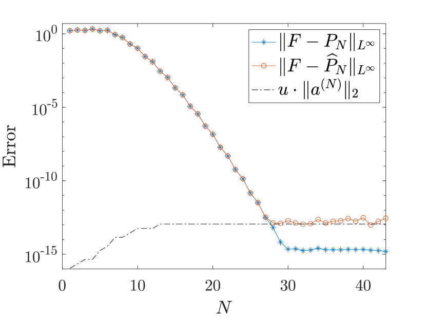
(a) $F(x)=\cos(8x+1)$

(b) $F(x)=\cos(12x+1)$

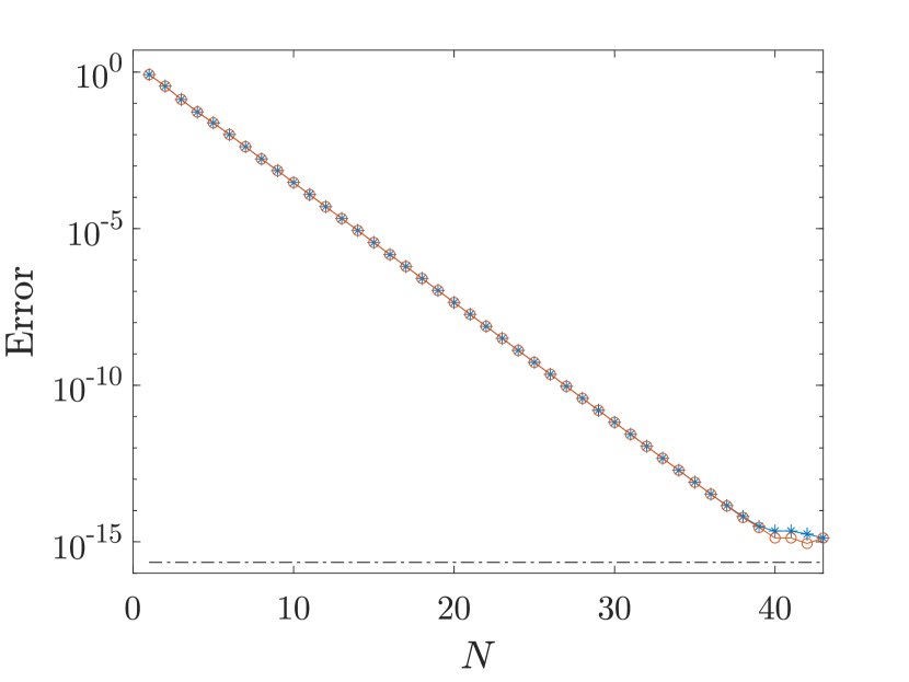
(c) $F(x)=\frac{1}{x-\sqrt{2}}$

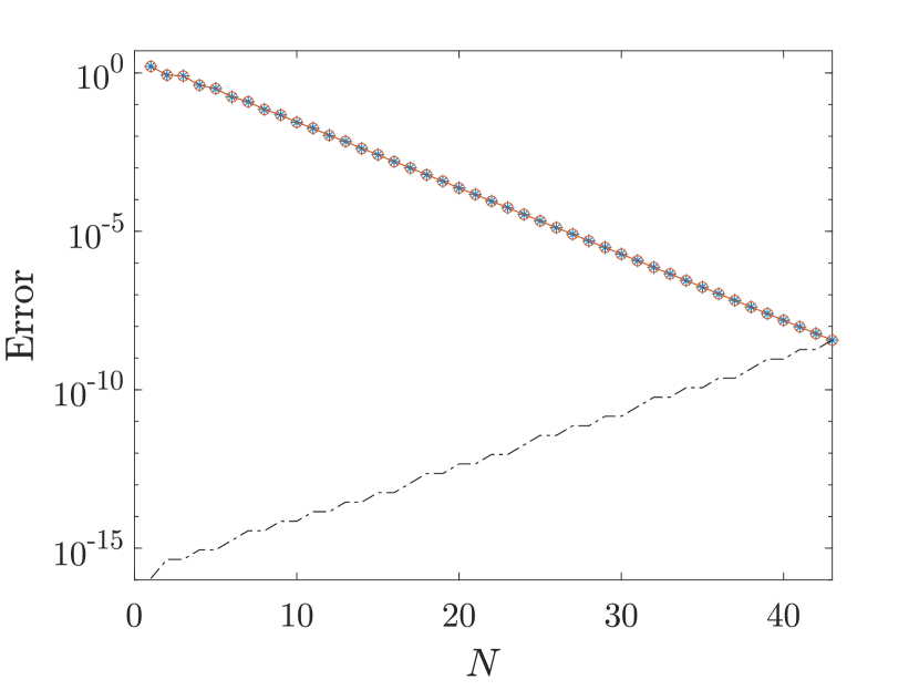
(d) $F(x)=\frac{1}{x-0.5i}$

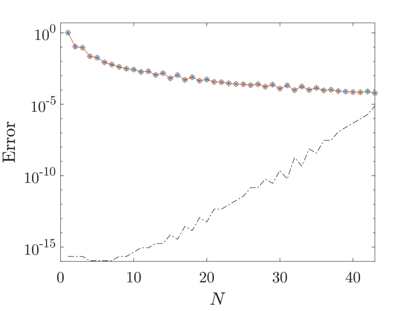
(e) ${\lvert x+0.1\rvert}^{2.5}$

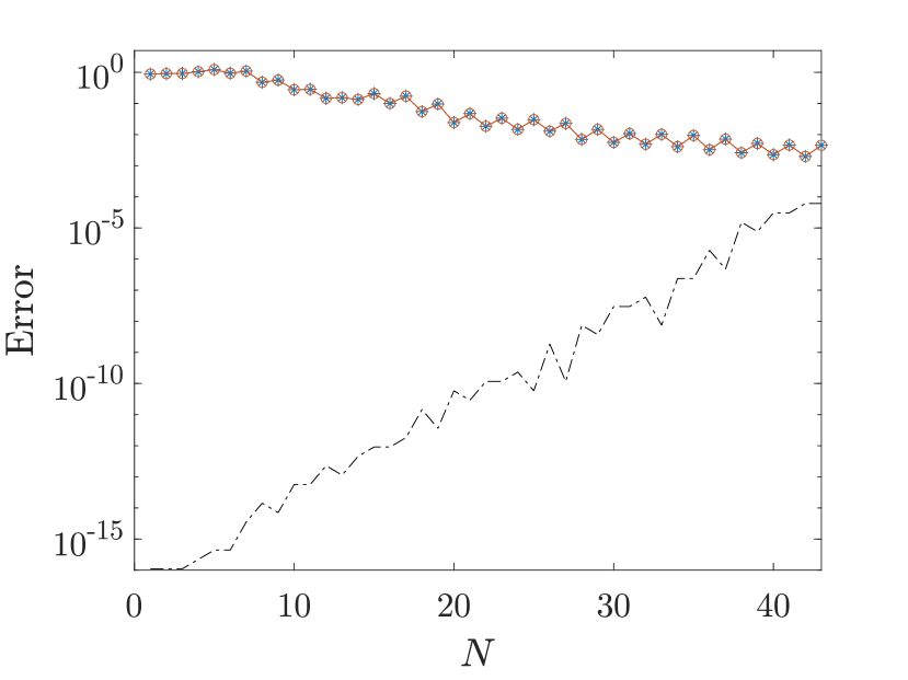
(f) ${\lvert\sin(5x)\rvert}^{3}$

Figure 5: Polynomial interpolation error, monomial approximation error and $u\cdot{\lVert a^{(N)}\rVert}_{2}$. These functions are the ones that appear in Section 1.

Remark 2.1.

The second term on the right-hand side of (16) is an upper bound of the backward error ${\lVert P_{N}-\widehat{P}_{N}\rVert}_{L^{\infty}(\Gamma)}$, i.e., the extra loss of accuracy caused by the use of a monomial basis. Note that the absolute condition number of the evaluation of $P_{N}(z)$ in the monomial basis is around ${\lVert a^{(N)}\rVert}_{2}$ when ${\lvert z\rvert}\approx 1$, so that the resulting error is bounded by $u\cdot{\lVert a^{(N)}\rVert}_{2}$, which is always smaller than $2u\cdot\gamma_{N}\Lambda_{N}{\lVert a^{(N)}\rVert}_{2}$.

The rest of this section is structured as follows. First, we review a classical result on function approximation over a smooth simple arc $\Gamma\subset\mathbbm{C}$ by polynomials. Next, we study the backward error ${\lVert P_{N}-\widehat{P}_{N}\rVert}_{L^{\infty}(\Gamma)}$ by bounding the 2-norm of the monomial coefficients of the interpolating polynomial. Finally, we study the growth of ${\lVert(V^{(N)})^{-1}\rVert}_{2}$, which determines the validity of the condition on the a priori error estimate (16).

Below, we define a generalization of the Bernstein ellipse, to the case of a smooth simple arc in the complex plane.

Definition 2.1.

Given a smooth simple arc $\Gamma$ in the complex plane, we define $E_{\rho}$ to be the level set $\{x+iy\in\mathbbm{C}:G(x,y)=\log\rho\}$, where $G:\mathbbm{R}^{2}\to\mathbbm{R}$ is the unique solution to the exterior Laplace equation

$$\nabla^{2}G= \,0\text{ in }\mathbbm{R}^{2}\setminus\Gamma,$$

$$G= \,0\text{ on }\partial\Gamma,$$

$$G(x)\sim \,\log{\lvert x\rvert}\text{ as }{\lvert x\rvert}\to\infty.$$ (20)

Furthermore, we let $E_{\rho}^{o}$ denote the open region bounded by $E_{\rho}$.

We note that, when $\Gamma=[a,b]\subset\mathbbm{R}$, the level set $E_{\rho}$ is a Bernstein ellipse with parameter $\rho$, with foci at $a$ and $b$. In Figure 6, we plot examples of level sets $E_{\rho}$ for an interval and for a sine curve, for various values of $\rho$.

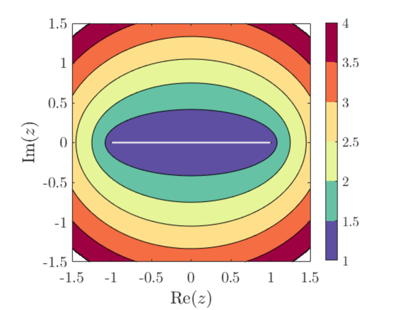
(a) $\Gamma=[-1,1]$

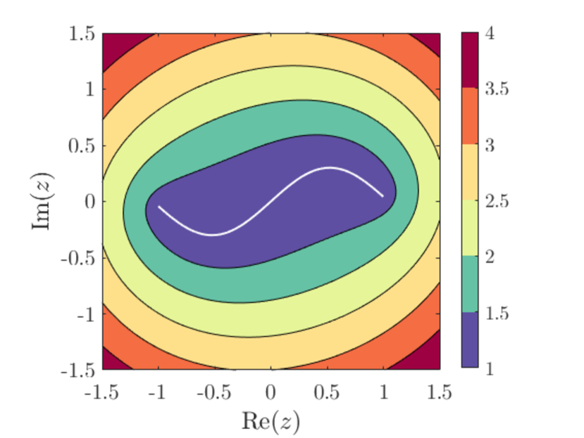
(b) $\Gamma=\left\{t+0.3i\sin(3t):t\in[-1,1]\right\}$

Figure 6: The level set $E_{\rho}$ corresponding to $\Gamma$, for various values of $\rho$. The colorbar indicates the value of $\rho$. The smooth simple arc $\Gamma$ is the white curve in the figure. The plots were made using the source code provided in [2].

The following theorem illustrates just one situation where function approximation by polynomials over a smooth simple arc $\Gamma$ in the complex plane is feasible. We refer the readers to Section 4.5 in [28] for the proof.

Theorem 2.3.

Let $\Gamma$ be a smooth simple arc in the complex plane. Suppose that the function $F:\Gamma\to\mathbbm{C}$ is analytically continuable to the closure of the region $E_{\rho}^{o}$ corresponding to $\Gamma$, for some $\rho>1$. Then, there exists a sequence of polynomials $\{Q_{n}\}$ satisfying

$${\lVert F-Q_{n}\rVert}_{L^{\infty}(\Gamma)}\leq C\rho^{-n},$$ (21)

for all $n\geq 0$, where $C\geq 0$ is a constant that is independent of $N$.

Remark 2.2.

When $\Gamma$ is a line segment, the magnitude of the constant $C$ in (21) is proportional to ${\lVert F\rVert}_{L^{\infty}(E_{\rho}^{o})}$ (see Theorem 2.8 in Section 2.3). We conjecture that the same holds in the general case.

The parameter $\rho_{*}$ defined below appears in our bounds for both the 2-norm of the monomial coefficient vector of the interpolating polynomial, and the growth rate of the 2-norm of the inverse of a Vandermonde matrix. It denotes the parameter of the smallest region $E_{\rho}^{o}$ that contains the open unit disk centered at the origin.

Definition 2.2.

Given a smooth simple arc $\Gamma\subset\mathbbm{C}$, define $\rho_{*}:=\inf\{\rho>1:D_{1}\subset E_{\rho}^{o}\}$, where $D_{1}$ is the open unit disk centered at the origin, and $E_{\rho}^{o}$ is the region corresponding to $\Gamma$ (see Definition 2.1).

The following lemma provides upper bounds for the 2-norm of the monomial coefficient vector of an arbitrary polynomial.

Lemma 2.4.

Let $P_{N}:\mathbbm{C}\to\mathbbm{C}$ be a polynomial of degree $N$, where $P_{N}(z)=\sum_{k=0}^{N}a_{k}z^{k}$ for some $a_{0},a_{1},\dots,a_{N}\in\mathbbm{C}$. The 2-norm of the coefficient vector $a^{(N)}:=(a_{0},a_{1},\dots,a_{N})^{T}$ satisfies

$${\lVert a^{(N)}\rVert}_{2}\leq{\lVert P_{N}\rVert}_{L^{\infty}(\partial D_{1})}\leq\rho_{*}^{N}{\lVert P_{N}\rVert}_{L^{\infty}(\Gamma)},$$ (22)

where $D_{1}$ denotes the open unit disk centered at the origin, and $\rho_{*}$ is given in Definition 2.2.

Proof. Observe that $P_{N}(e^{i\theta})=\sum_{k=0}^{N}a_{k}e^{ik\theta}$. By Parseval’s identity, we have that

$${\lVert a^{(N)}\rVert}_{2}=\Bigl{(}\frac{1}{2\pi}\int_{0}^{2\pi}{\lvert P_{N}(e^{i\theta})\rvert}^{2}\,\mathrm{d}\theta\Bigr{)}^{1/2}\leq{\lVert P_{N}\rVert}_{L^{\infty}(\partial D_{1})}\leq{\lVert P_{N}\rVert}_{L^{\infty}(E_{\rho_{*}}^{o})},$$ (23)

where the last inequality comes from the fact that $D_{1}\subset E_{\rho_{*}}^{o}$ (see Definition 2.1). Finally, based on one of Bernstein’s inequalities (see Section 4.6 in [28]), we have

$${\lVert P_{N}\rVert}_{L^{\infty}(E_{\rho_{*}}^{o})}\leq\rho_{*}^{N}{\lVert P_{N}\rVert}_{L^{\infty}(\Gamma)}.$$ (24)

$\blacksquare$

The following theorem provides an upper bound for the 2-norm of the monomial coefficients of an arbitrary interpolating polynomial.

Theorem 2.5.

Let $\Gamma$ be a smooth simple arc in the complex plane, and let $F:\Gamma\to\mathbbm{C}$ be an arbitrary function. Suppose that there exists a finite sequence of polynomials $\{Q_{n}\}_{n=0,1,\dots,N}$, where $Q_{n}$ has degree $n$, which satisfies

$${\lVert F-Q_{n}\rVert}_{L^{\infty}(\Gamma)}\leq C_{N}\rho^{-n},\quad 0\leq n\leq N,$$ (25)

for some constants $\rho>1$ and $C_{N}\geq 0$. Define $P_{N}(z)=\sum_{k=0}^{N}a_{k}z^{k}$ to be the $N$th degree interpolating polynomial of $F$ for a given set of distinct collocation points $Z=\{z_{j}\}_{j=0,1,\dots,N}\subset\Gamma$. The 2-norm of the monomial coefficient vector $a^{(N)}:=(a_{0},a_{1},\dots,a_{N})^{T}$ of $P_{N}$ satisfies

$${\lVert a^{(N)}\rVert}_{2}\leq{\lVert F\rVert}_{L^{\infty}(\Gamma)}+C_{N}\Bigl{(}\Lambda_{N}\Bigl{(}\frac{\rho_{*}}{\rho}\Bigr{)}^{N}+2\rho_{*}\sum_{j=0}^{N-1}\Bigl{(}\frac{\rho_{*}}{\rho}\Bigr{)}^{j}+1\Bigr{)},$$ (26)

where $\rho_{*}$ is given in Definition 2.2, and $\Lambda_{N}$ denotes the Lebesgue constant for $Z$.

Proof. Given $n\geq 0$, let $M^{(n)}:\mathbbm{R}^{n+1}\to\mathcal{P}_{n}$ be the bijective linear map associating each vector $(u_{0},u_{1},\dots,u_{n})^{T}\in\mathbbm{R}^{n+1}$ with the $n$th degree polynomial $\sum_{k=0}^{n}u_{k}z^{k}\in\mathcal{P}_{n}$. It follows immediately from Lemma 2.4 that, given any polynomial $P\in\mathcal{P}_{n}$,

$${\bigl{\lVert}(M^{(n)})^{-1}[P]\bigr{\rVert}}_{2}\leq\rho_{*}^{n}{\lVert P\rVert}_{L^{\infty}(\Gamma)}.$$ (27)

Therefore, by the triangle inequality, the 2-norm of the monomial coefficient vector of the polynomial $Q_{N}$ satisfies

$${\bigl{\lVert}(M^{(N)})^{-1}[Q_{N}]\bigr{\rVert}}_{2}\leq\, {\bigl{\lVert}(M^{(N)})^{-1}[Q_{0}]\bigr{\rVert}}_{2}+\sum_{j=0}^{N-1}{\bigl{\lVert}(M^{(N)})^{-1}[Q_{j+1}-Q_{j}]\bigr{\rVert}}_{2}$$

$$=\, {\lVert Q_{0}\rVert}_{L^{\infty}(\Gamma)}+\sum_{j=0}^{N-1}{\bigl{\lVert}(M^{(j+1)})^{-1}[Q_{j+1}-Q_{j}]\bigr{\rVert}}_{2}$$

$$\leq\, \bigl{(}{\lVert F\rVert}_{L^{\infty}(\Gamma)}+C_{N}\bigr{)}+\sum_{j=0}^{N-1}\rho_{*}^{j+1}{\left\|Q_{j+1}-Q_{j}\right\|}_{L^{\infty}(\Gamma)}$$

$$\leq\, \bigl{(}{\lVert F\rVert}_{L^{\infty}(\Gamma)}+C_{N}\bigr{)}+2C_{N}\rho_{*}\sum_{j=0}^{N-1}\Bigl{(}\frac{\rho_{*}}{\rho}\Bigr{)}^{j},$$ (28)

from which it follows that ${\lVert a^{(N)}\rVert}_{2}$ satisfies

$${\lVert a^{(N)}\rVert}_{2}\leq\, {\bigl{\lVert}(M^{(N)})^{-1}[P_{N}-Q_{N}]\bigr{\rVert}}_{2}+{\bigl{\lVert}(M^{(N)})^{-1}[Q_{N}]\bigr{\rVert}}_{2}$$

$$\leq\, \rho_{*}^{N}{\lVert P_{N}-Q_{N}\rVert}_{L^{\infty}(\Gamma)}+{\bigl{\lVert}(M^{(N)})^{-1}[Q_{N}]\bigr{\rVert}}_{2}$$

$$\leq\, \rho_{*}^{N}\Lambda_{N}{\lVert F-Q_{N}\rVert}_{L^{\infty}(\Gamma)}+{\bigl{\lVert}(M^{(N)})^{-1}[Q_{N}]\bigr{\rVert}}_{2}$$

$$\leq\, {\lVert F\rVert}_{L^{\infty}(\Gamma)}+C_{N}\Bigl{(}\Lambda_{N}\Bigl{(}\frac{\rho_{*}}{\rho}\Bigr{)}^{N}+2\rho_{*}\sum_{j=0}^{N-1}\Bigl{(}\frac{\rho_{*}}{\rho}\Bigr{)}^{j}+1\Bigr{)},$$ (29)

where the third inequality comes from the observation that $P_{N}-Q_{N}$ is the interpolating polynomial of $F-Q_{N}$ for the set of collocation points $Z$. $\blacksquare$

Remark 2.3.

The assumption (25) made in the theorem above can be satisfied for any function $F$ by choosing $C_{N}$ to be sufficiently large. When the function $F$ is continuable to the closure of the region $E_{\rho}^{o}$ corresponding to $\Gamma$ (see Definition 2.1), for some $\rho>\rho_{*}$, one can show that ${\lVert a^{(N)}\rVert}_{2}\leq 2{\lVert F\rVert}_{L^{\infty}(\partial D_{1})}$, where $D_{1}$ is defined in Definition 2.2. This result comes from a generalization of Theorem 2.3 (see [10]), which says that ${\lVert F-P_{N}\rVert}_{L^{\infty}(E_{\rho_{*}}^{o})}=\mathcal{O}\bigl{(}(\rho_{*}/\rho)^{N}\bigr{)}$, from which it follows that

$${\lVert a^{(N)}\rVert}_{2}\leq{\lVert P_{N}\rVert}_{L^{\infty}(\partial D_{1})}\leq{\lVert P_{N}-F\rVert}_{L^{\infty}(\partial D_{1})}+{\lVert F\rVert}_{L^{\infty}(\partial D_{1})}\leq 2{\lVert F\rVert}_{L^{\infty}(\partial D_{1})}.$$ (30)

The following theorem bounds the growth of the 2-norm of the inverse of a Vandermonde matrix.

Theorem 2.6.

Suppose that $V^{(N)}\in\mathbbm{C}^{(N+1)\times(N+1)}$ is a Vandermonde matrix with $(N+1)$ distinct collocation points $Z=\{z_{j}\}_{j=0,1,\dots,N}\subset\mathbbm{C}$. Suppose further that $\Gamma\subset\mathbbm{C}$ is a smooth simple arc such that $Z\subset\Gamma$. The 2-norm of $(V^{(N)})^{-1}$ is bounded by

$${\lVert(V^{(N)})^{-1}\rVert}_{2}\leq\rho_{*}^{N}\Lambda_{N},$$ (31)

where $\rho_{*}$ is given in Definition 2.2, and $\Lambda_{N}$ denotes the Lebesgue constant for the set of collocation points $Z$ over $\Gamma$.

Proof. Let $f^{(N)}=(f_{0},f_{1},\dots,f_{N})^{T}\in\mathbbm{C}^{N+1}$ be an arbitrary vector. Suppose that $P_{N}$ is an interpolating polynomial of degree $N$ for the set $\{(z_{j},f_{j})\}_{j=0,1,\dots,N}$. By Lemma 2.4, the 2-norm of the monomial coefficient vector $a^{(N)}$ of $P_{N}$ satisfies

$${\lVert a^{(N)}\rVert}_{2}\leq\rho_{*}^{N}{\lVert P_{N}\rVert}_{L^{\infty}(\Gamma)}\leq\rho_{*}^{N}\Lambda_{N}{\lVert f^{(N)}\rVert}_{\infty}\leq\rho_{*}^{N}\Lambda_{N}{\lVert f^{(N)}\rVert}_{2},$$ (32)

where the second inequality follows from the definition of the Lebesgue constant. Therefore, the 2-norm of $(V^{(N)})^{-1}$ is bounded by

$${\lVert(V^{(N)})^{-1}\rVert}_{2}=\sup_{f^{(N)}\neq 0}\Bigl{\{}\frac{{\lVert(V^{(N)})^{-1}f^{(N)}\rVert}_{2}}{{\lVert f^{(N)}\rVert}_{2}}\Bigr{\}}=\sup_{f^{(N)}\neq 0}\Bigl{\{}\frac{{\lVert a^{(N)}\rVert}_{2}}{{\lVert f^{(N)}\rVert}_{2}}\Bigr{\}}\leq\rho_{*}^{N}\Lambda_{N}.$$ (33)

$\blacksquare$

Note that the bound above applies to any smooth simple arc $\Gamma\subset\mathbbm{C}$ that contains the set of collocation points $Z$.

Observation 2.4.

In the case where the set of $(N+1)$ collocation points $Z\subset\Gamma$ are chosen such that the associated Lebesgue constant $\Lambda_{N}$ is small, we observe in practice that the upper bound $\rho_{*}^{N}\Lambda_{N}$ is reasonably close to the value of ${\lVert(V^{(N)})^{-1}\rVert}_{2}$ (see Figures 10 and 14(b) for numerical evidence).

Remark 2.5.

A worst case upper bound for ${\lVert a^{(N)}\rVert}_{2}$ is provided by inequality (32) in the proof of Theorem 2.6, as the right-hand side of this inequality is independent of the smoothness of the function $F$.

2.1 Under what conditions is interpolation in the monomial basis as good as interpolation in a well-conditioned polynomial basis?

Without loss of generality, we assume that the smooth simple arc $\Gamma$ is inside the unit disk centered at the origin (such that ${\lVert V^{(N)}\rVert}_{2}$ is small and $\gamma_{N}\lesssim 1$). Furthermore, we choose a set of $(N+1)$ collocation points $Z\subset\Gamma$ with a small Lebesgue constant $\Lambda_{N}$, and let $V^{(N)}$ denote the corresponding Vandermonde matrix. Recall from Theorem 2.2 that, if

$${\lVert(V^{(N)})^{-1}\rVert}_{2}\leq\frac{1}{2u\cdot\gamma_{N}},$$ (34)

then the monomial approximation error ${\lVert F-\widehat{P}_{N}\rVert}_{L^{\infty}(\Gamma)}$ is bounded a priori by

$${\lVert F-\widehat{P}_{N}\rVert}_{L^{\infty}(\Gamma)}\lesssim{\lVert F-P_{N}\rVert}_{L^{\infty}(\Gamma)}+u\cdot{\lVert a^{(N)}\rVert}_{2},$$ (35)

where $u$ denotes machine epsilon, $\widehat{P}_{N}$ is the computed monomial expansion, $P_{N}$ is the exact $N$th degree interpolating polynomial of $F$ for the set of collocation points $Z$, and $a^{(N)}$ is the monomial coefficient vector of $P_{N}$.

By Theorem 2.5, if there exists a constant $C_{N}\geq 0$ and a finite sequence of polynomials $\{Q_{n}\}_{n=0,1,\dots,N}$ such that ${\lVert F-Q_{n}\rVert}_{L^{\infty}(\Gamma)}\leq C_{N}\rho_{*}^{-n}$ for $0\leq n\leq N$, where $Q_{n}$ has degree $n$ and $\rho_{*}$ is given in Definition 2.2, then the monomial coefficient vector $a^{(N)}$ of $P_{N}$ satisfies

$${\lVert a^{(N)}\rVert}_{2}\lesssim C_{N}\Lambda_{N}N\approx C_{N},$$ (36)

and inequality (35) becomes

$${\lVert F-\widehat{P}_{N}\rVert}_{L^{\infty}(\Gamma)}\lesssim \,{\lVert F-P_{N}\rVert}_{L^{\infty}(\Gamma)}+u\cdot C_{N}.$$ (37)

In practice, one can take $\{Q_{n}\}_{n=0,1,\dots,N}$ to be a finite sequence of interpolating polynomials $\{P_{n}\}_{n=0,1,\dots,N}$ of $F$ for sets of collocation points with small Lebesgue constants. When the Lebesgue constant $\Lambda_{N}$ is small, it follows from Theorem 2.6 that the condition (34) is satisfied when $\rho_{*}^{N}\lesssim\frac{1}{u}$. We assume here that $N$ is sufficiently small so that $\rho_{*}^{N}\lesssim\frac{1}{u}$. Without loss of generality, we assume that the upper bound for ${\lVert F-P_{n}\rVert}_{L^{\infty}(\Gamma)}$, i.e., $C_{N}\rho_{*}^{-n}$, is tight, in the sense that there exists some integer $n\in[0,N]$ such that ${\lVert F-P_{n}\rVert}_{L^{\infty}(\Gamma)}=C_{N}\rho_{*}^{-n}$. Note that the smallest uniform approximation error we can hope to obtain in practice is $u\cdot{\lVert F\rVert}_{L^{\infty}(\Gamma)}$.

When $u\cdot C_{N}\lesssim\max({\lVert F-P_{N}\rVert}_{L^{\infty}(\Gamma)},u\cdot{\lVert F\rVert}_{L^{\infty}(\Gamma)})$, the use of a monomial basis for interpolation introduces essentially no extra error. Interestingly, this happens both if the polynomial interpolation error decays quickly and if the polynomial interpolation error decays slowly. Suppose that the polynomial interpolation error decays quickly, so that the bound is tight for $n=0$, i.e., ${\lVert F-P_{0}\rVert}_{L^{\infty}(\Gamma)}=C_{N}$. Since $C_{N}\lesssim 2{\lVert F\rVert}_{L^{\infty}(\Gamma)}$, we see that the extra error caused by the use of a monomial basis is bounded by $u\cdot C_{N}\lesssim 2u\cdot{\lVert F\rVert}_{L^{\infty}(\Gamma)}\lesssim u\cdot{\lVert F\rVert}_{L^{\infty}(\Gamma)}$. Examples of this situation are illustrated in Figure 7. Suppose now that the polynomial interpolation error decays slowly, so that bound is tight for $n=N$, i.e., ${\lVert F-P_{N}\rVert}_{L^{\infty}(\Gamma)}=C_{N}\rho_{*}^{-N}$. Since we assumed that $\rho_{*}^{N}\lesssim\frac{1}{u}$, it follows that $u\cdot C_{N}\lesssim{\lVert F-P_{N}\rVert}_{L^{\infty}(\Gamma)}$. Examples of this situation are illustrated in Figure 8.

When $u\cdot C_{N}\gtrsim\max({\lVert F-P_{N}\rVert}_{L^{\infty}(\Gamma)},u\cdot{\lVert F\rVert}_{L^{\infty}(\Gamma)})$, stagnation of convergence can occur. In practice, we observe that the extra error caused by the use of the monomial basis, i.e., $u\cdot{\lVert a^{(N)}\rVert}_{2}$, is close to $u\cdot C_{N}$, so the monomial approximation error ${\lVert F-\widehat{P}_{N}\rVert}_{L^{\infty}(\Gamma)}$ generally stagnates at an error level around $u\cdot C_{N}$. Note that a slow decay in ${\lVert F-P_{n}\rVert}_{L^{\infty}(\Gamma)}$ results in a larger value of $C_{N}$, while a fast decay in ${\lVert F-P_{n}\rVert}_{L^{\infty}(\Gamma)}$ favors a smaller final interpolation error ${\lVert F-P_{N}\rVert}_{L^{\infty}(\Gamma)}$. This means that, for stagnation of convergence to occur, the polynomial interpolation error has to exhibit some combination of slow decay followed by fast decay. Furthermore, note that an upper bound for $C_{N}$ is given by $C_{N}\lesssim\rho_{*}^{N}$ (see Remark 2.5). This means that, the smaller the value of $N$, the smaller the maximum possible value of $C_{N}$, and the more rapid the rate of decay in ${\lVert F-P_{n}\rVert}_{L^{\infty}(\Gamma)}$ required for stagnation of convergence to occur. We present examples of this situation in Figure 9.

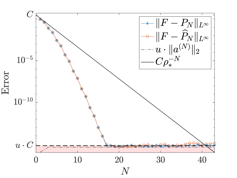
(a) $\cos(2x+1)$, $C=3\times 10^{0}$

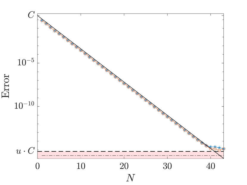
(b) $\frac{1}{x-\sqrt{2}}$, $C=3\times 10^{0}$

Figure 7: The extra error caused by the use of a monomial basis is negligible. The pink region denotes the bound for $u\cdot{\lVert a^{(n)}\rVert}_{2}$

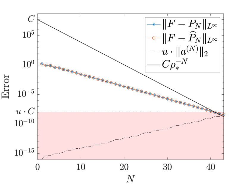
(a) $\frac{1}{x-0.5i}$, $C=5\times 10^{7}$

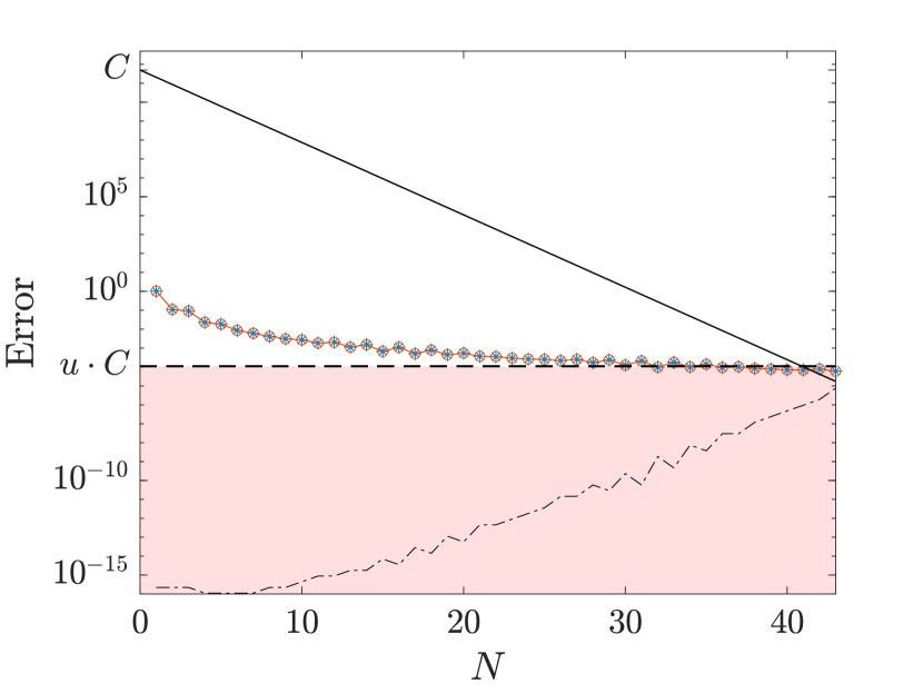
(b) ${\lvert x+0.1\rvert}^{2.5}$, $C=5\times 10^{11}$

Figure 8: The extra error caused by the use of a monomial basis is no larger than ${\lVert F-P_{N}\rVert}_{L^{\infty}(\Gamma)}$. The pink region denotes the bound for $u\cdot{\lVert a^{(n)}\rVert}_{2}$

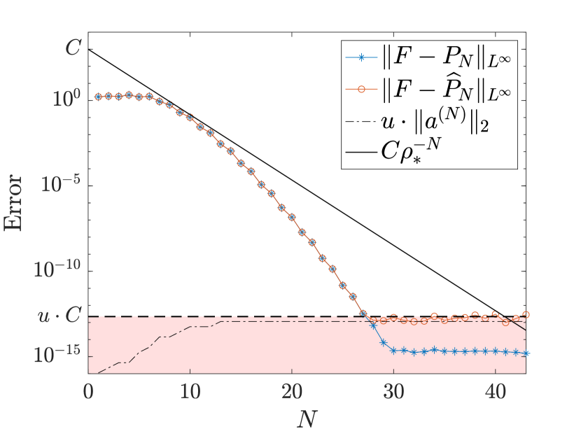
(a) $\cos(8x+1)$, $C=1\times 10^{3}$

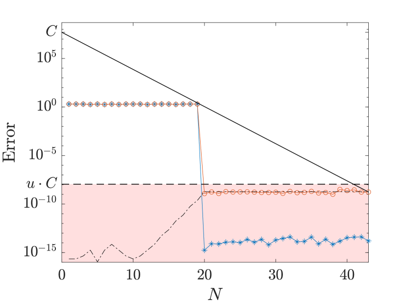
(b) $F(x)=T_{20}(x)$, $C=5\times 10^{7}$

Figure 9: Stagnation of convergence. The pink region denotes the bound for $u\cdot{\lVert a^{(n)}\rVert}_{2}$.

2.2 Practical use of a monomial basis for interpolation

What are the restrictions on polynomial interpolation in the monomial basis? Firstly, extremely high-order global interpolation is impossible in the monomial basis, because the order $N$ must satisfy ${\lVert(V^{(N)})^{-1}\rVert}_{2}\lesssim\frac{1}{u}$ for our estimates to hold, where $u$ denotes machine epsilon. In fact, even if this condition were not required, there would still be no benefit in taking an order larger than this threshold. This is because, in almost all situations, the extra error caused by the use of the monomial basis dominates the monomial approximation error when ${\lVert(V^{(N)})^{-1}\rVert}_{2}>\frac{1}{u}$, leading to a stagnation of convergence.

On the other hand, piecewise polynomial interpolation in the monomial basis over a partition of $\Gamma$ can be carried out stably, provided that the maximum order of approximation over each subpanel is maintained below the threshold $\operatorname*{arg\,max}_{N}{\lVert(V^{(N)})^{-1}\rVert}_{2}\lesssim\frac{1}{u}$, and that the size of $u\cdot{\lVert a^{(N)}\rVert}_{2}\approx u\cdot{\lVert\widehat{a}^{(N)}\rVert}_{2}$ is kept below the size of the polynomial interpolation error, where $a^{(N)}$ and $\widehat{a}^{(N)}$ denote the exact and the computed monomial coefficient vectors, respectively. As demonstrated in Section 2.1, the latter requirement is often satisfied automatically, and when it is not, adding an extra level of subdivision almost always resolves the issue. In addition, the extra error caused by the use of a monomial basis can always be estimated promptly during computation, using the value of $u\cdot{\lVert\widehat{a}^{(N)}\rVert}_{2}$.

Based on the discussion above, we summarize the proper way of using the monomial basis for interpolation as follows. For simplicity, we use the same order of approximation over each subpanel, and denote the order using $N$. Firstly, $N$ needs to be smaller than the threshold $\operatorname*{arg\,max}_{N}{\lVert(V^{(N)})^{-1}\rVert}_{2}\lesssim\frac{1}{u}$. Then, given a function $F:\Gamma\to\mathbbm{C}$ and an error tolerance $\varepsilon$, we subdivide the domain $\Gamma$ until $F$ can be approximated by a polynomial of degree less than $N$ over each subpanel to within an error of $\varepsilon$. Finally, we subdivide the panels further until the norm of the monomial coefficients is less than $\varepsilon/u$ over each subpanel.

Since the convergence rate of piecewise polynomial approximation is $\mathcal{O}(h^{N+1})$, where $h$ and $N$ denote the maximum diameter and minimum order of approximation over all subpanels, respectively, and since the aforementioned threshold is generally not small (e.g., the threshold is approximately equal to $43$ when $\Gamma=[-1,1]$), piecewise polynomial interpolation in the monomial basis converges rapidly so long as we set the value of $N$ to be large enough. Therefore, there is no need to avoid the use of a monomial basis when it offers an advantage over other bases.

Remark 2.6.

It takes $\mathcal{O}(N^{3})$ operations to solve a Vandermonde system of size $N\times N$ by a standard backward stable solver, e.g., LU factorization with partial pivoting. Since the order of approximation $N$ is almost always not large, the solution to the Vandermonde matrix can be computed accurately, in the sense that $\gamma_{N}$ is small, and rapidly, using highly optimized linear algebra libraries, e.g., LAPACK. There also exist specialized algorithms that solve Vandermonde systems in $\mathcal{O}(N^{2})$ operations, e.g., the Björck-Pereyra algorithm [9], the Parker-Traub algorithm [15].

Observation 2.7.

What happens when the order of approximation exceeds the threshold? We observe that, despite that our theory is no longer applicable, the monomial approximation error does not become much larger than the error at the threshold, when the columns of the Vandermonde matrix are ordered as in (4) and when the system is solved by MATLAB’s backslash operator (which implements LU factorization with partial pivoting).

2.3 Interpolation over an interval

In this section, we consider polynomial interpolation in the monomial basis over an interval $\Gamma=[a,b]\subset\mathbbm{R}$. We suggest the use of the Chebyshev points on the interval $[a,b]$ as the collocation points, because of the following two well-known theorems related to Chebyshev approximation.

The theorem below, originally proved in [12], bounds the growth rate of the Lebesgue constant for the Chebyshev points.

Theorem 2.7.

Let $\Lambda_{N}$ be the Lebesgue constant for the $(N+1)$ Chebyshev points on an interval $[a,b]$. For any nonnegative integer $N$, the Lebesgue constant $\Lambda_{N}$ satisfies $\Lambda_{N}\leq\frac{2}{\pi}\log(N+1)+1$.

The following theorem provides a sufficient condition for the Chebyshev interpolant of a function to converge geometrically. The proof can be found in, for example, Theorem 8.2 in [27]. Recall that the level set $E_{\rho}$ for an interval $[a,b]$ is a Bernstein ellipse with parameter $\rho$, with foci at $a$ and $b$ (see Figure 6(a)).

Theorem 2.8.

Suppose that $F:[a,b]\to\mathbbm{C}$ is analytically continuable to the region $E_{\rho}^{o}$ (see Definition 2.1), and satisfies ${\lVert F\rVert}_{L^{\infty}(E_{\rho}^{o})}\leq M$ for some $M\geq 0$. The $N$th degree Chebyshev interpolant $P_{N}$ of $F$ satisfies

$${\lVert F-P_{N}\rVert}_{L^{\infty}([a,b])}\leq\frac{4M}{\rho-1}\rho^{-N},$$ (38)

for all $N\geq 0$.

We note that the theorem above is stronger than Theorem 2.3 when $\Gamma$ is an interval, as it specifies the constant factor $C$.

Remark 2.8.

The Legendre points exhibit similar characteristics to the Chebyshev points, and can also be effectively utilized for interpolation over an interval.

In the rest of this section, we provide a series of numerical experiments involving interpolation over intervals. In Figure 10, we report the 2-norm of the inverse of the Vandermonde matrices with Chebyshev collocation points, for the domains $\Gamma=[-1,1]$ and $\Gamma=[0,1]$. Note that when $\Gamma=[-1,1]$, we have that $\rho_{*}=1+\sqrt{2}$ and ${\lVert(V^{(N)})^{-1}\rVert}_{2}\leq\frac{1}{u}$ for $N\leq 43$; when $\Gamma=[0,1]$, we have that $\rho_{*}=3+2\sqrt{2}$ and ${\lVert(V^{(N)})^{-1}\rVert}_{2}\leq\frac{1}{u}$ for $N\leq 22$. In Figure 11, we interpolate functions which can be resolved by a Chebyshev interpolant of degree $N\leq 43$ over $\Gamma=[-1,1]$. In addition to the estimated values of ${\lVert F-P_{N}\rVert}_{L^{\infty}([-1,1])}$ and ${\lVert F-\widehat{P}_{N}\rVert}_{L^{\infty}([-1,1])}$, we plot three additional curves in each figure: the estimated values of $u\cdot{\lVert a^{(N)}\rVert}_{2}$ based on inequality (15), the upper bound $C\rho_{*}^{N}$ for ${\lVert F-P_{N}\rVert}_{L^{\infty}([-1,1])}$, and the upper bound $u\cdot C$ for $u\cdot{\lVert a^{(N)}\rVert}_{2}$. In Figure 12, we provide similar experiments for the case where $\Gamma=[0,1]$. Based on these experimental results, one can observe that the convergence stagnates after the monomial approximation error ${\lVert F-\widehat{P}_{N}\rVert}_{L^{\infty}(\Gamma)}$ reaches $u\cdot{\lVert a^{(N)}\rVert}_{2}$, which implies that inequality (35) is sharp. In addition, the values of $u\cdot{\lVert a^{(N)}\rVert}_{2}$ are always within the upper bound $u\cdot C$, which is inline with our analysis in Section 2.1.

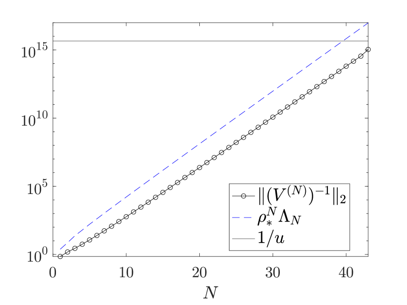
(a) $\Gamma=[-1,1]$

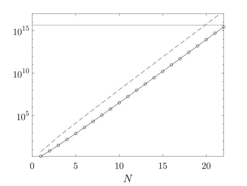
(b) $\Gamma=[0,1]$

Figure 10: The 2-norm of the inverse of a Vandermonde matrix with Chebyshev collocation points over an interval $\Gamma$, and its upper bound, for different orders of approximation. We note that $\rho_{*}=1+\sqrt{2}$ when $\Gamma=[-1,1]$, and $\rho_{*}=3+2\sqrt{2}$ when $\Gamma=[0,1]$.

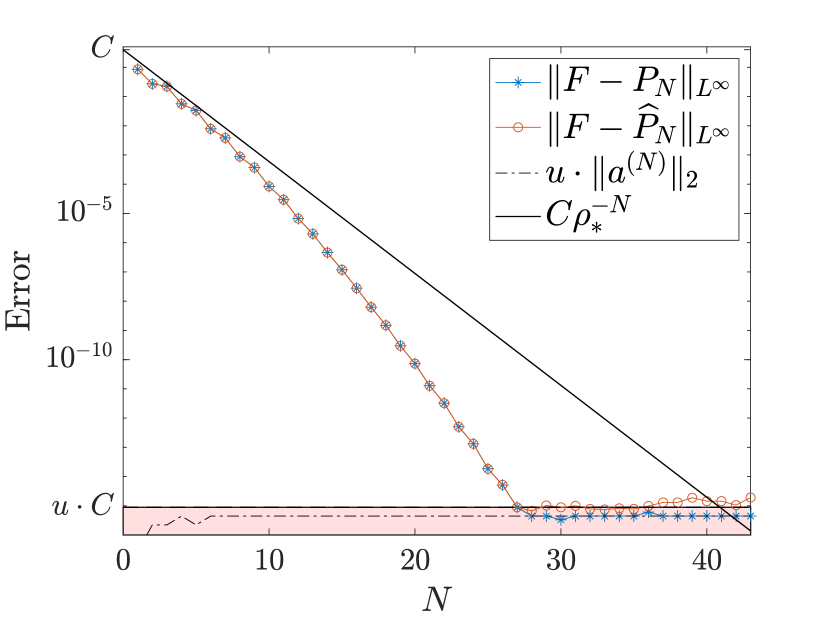
(a) $F(x)=e^{-2(x+0.1)^{2}}$, $C=4\times 10^{0}$

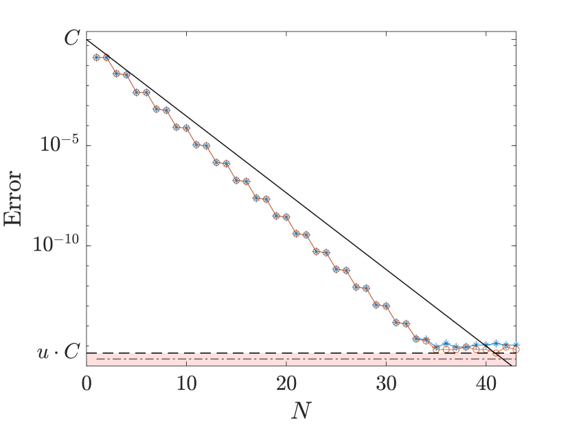
(b) $F(x)=\tan(x)$, $C=2\times 10^{0}$

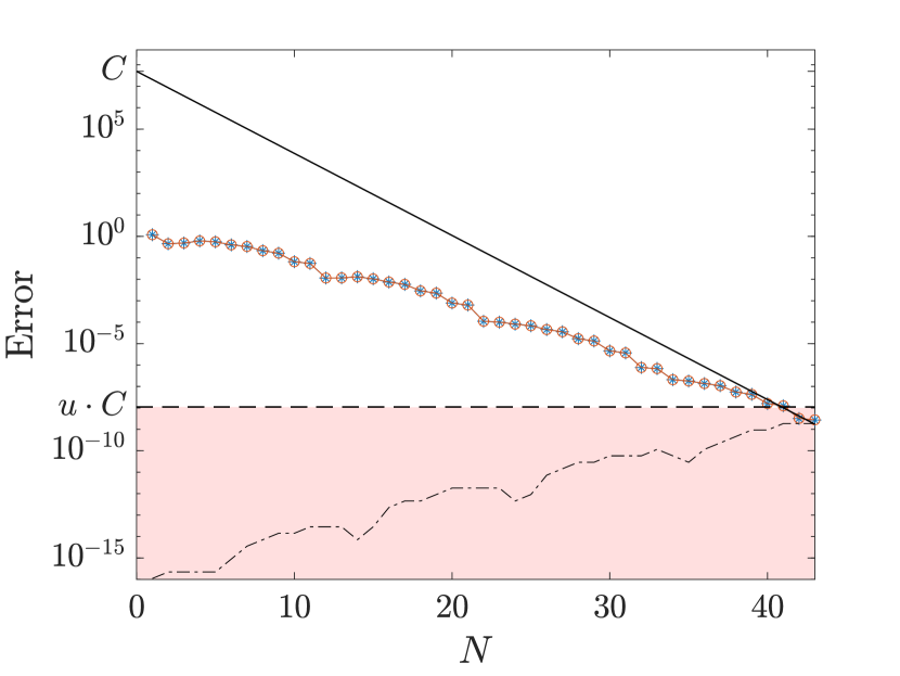
(c) $F(x)=\cos(3x^{8}+1)$, $C=5\times 10^{7}$

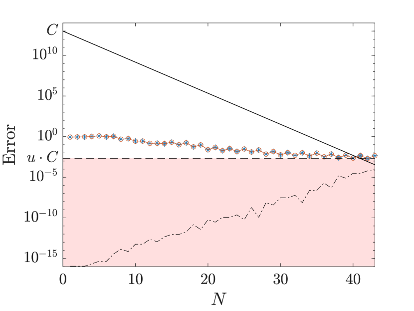
(d) $F(x)={\lvert\sin(5x)\rvert}^{3}$, $C=1\times 10^{13}$

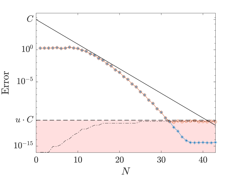
(e) $\cos(12x+1)$, $C=5\times 10^{4}$

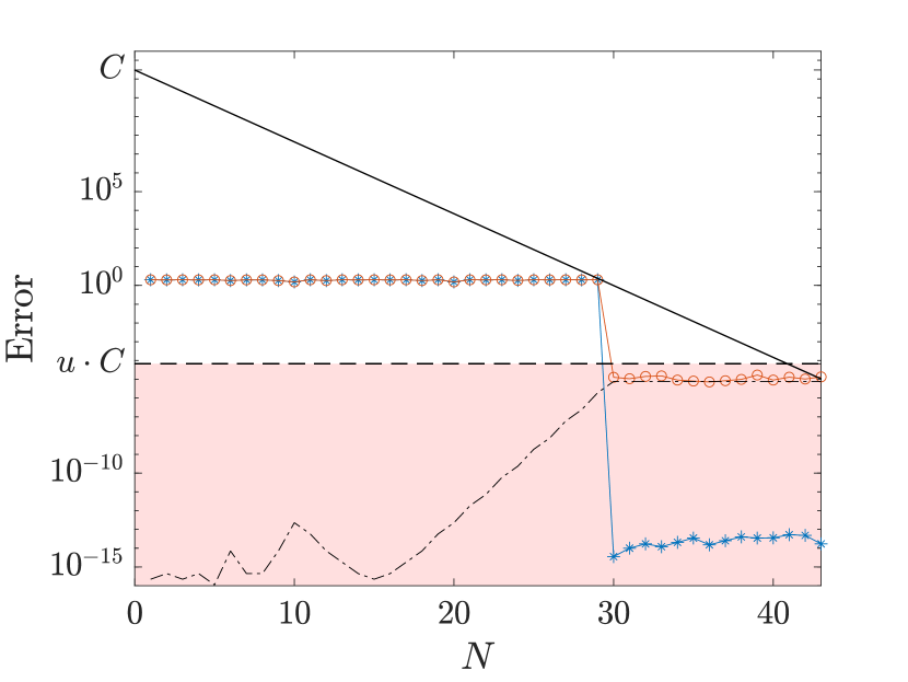
(f) $F(x)=T_{30}(x)$, $C=3\times 10^{11}$

Figure 11: Polynomial interpolation in the monomial basis over $\Gamma=[-1,1]$. The constant $\rho_{*}$ equals $1+\sqrt{2}$.

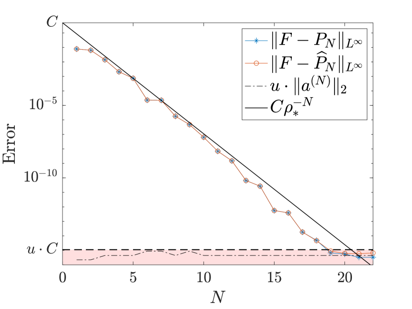
(a) $F(x)=e^{-2(x+0.1)^{2}}$, $C=5\times 10^{0}$

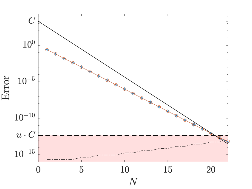
(b) $F(x)=\tan(x)$, $C=2\times 10^{3}$

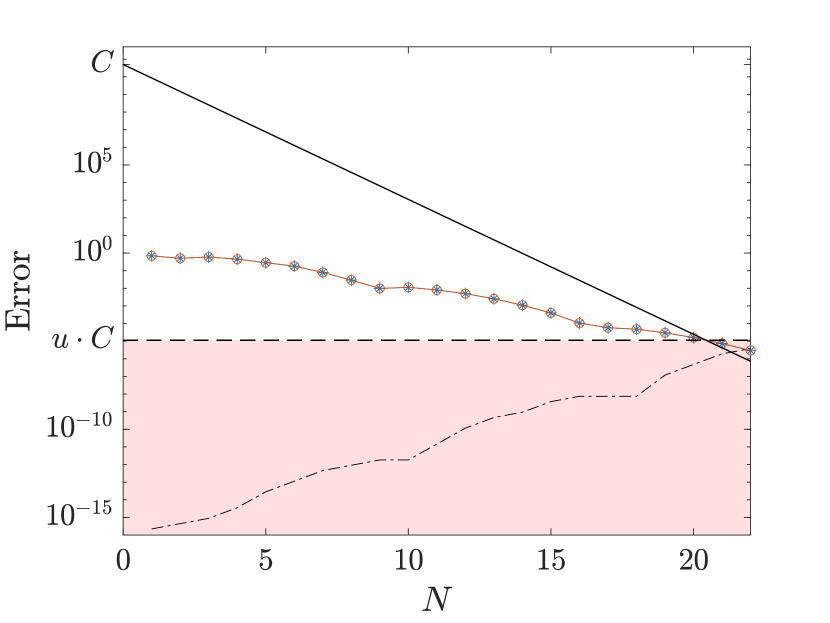
(c) $F(x)=\cos(3x^{8}+1)$, $C=5\times 10^{10}$

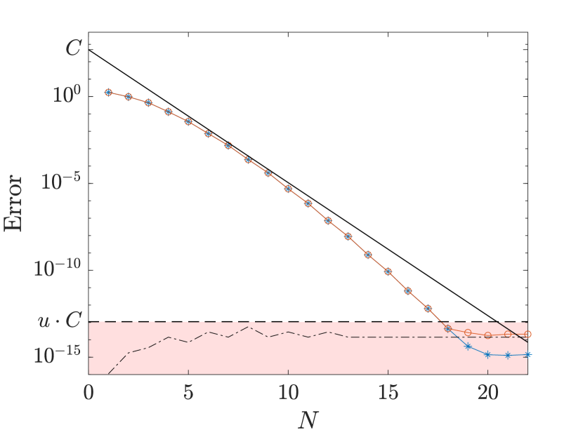
(d) $F(x)=\sin(6x+1)$, $C=5\times 10^{2}$

Figure 12: Polynomial interpolation in the monomial basis over $\Gamma=[0,1]$. The constant $\rho_{*}$ equals $3+2\sqrt{2}$.

2.4 Interpolation over a smooth simple arc in the complex plane

In this section, we consider polynomial interpolation in the monomial basis over a smooth simple arc $\Gamma\subset\mathbbm{C}$. In this more general setting, similar to the special case where $\Gamma$ is an interval, there exists a class of collocation points, known as adjusted Fejér points, whose associated Lebesgue constant also grows logarithmically [29]. However, these points are extremely costly to construct numerically. On the other hand, the set of collocation points constructed based on the following procedure, while suboptimal, is a good choice for practical applications. Suppose that $g:[-1,1]\to\mathbbm{C}$ is a parameterization of $\Gamma$. Provided that the Jacobian $g^{\prime}(t)$ does not have large variations, we find that the Lebesgue constant for the set of collocation points $Z=\{g(t_{j})\}_{j=0,1,\dots,N}$, where $\{t_{j}\}_{j=0,1,\dots,N}$ is the set of $(N+1)$ Chebyshev points on the interval $[-1,1]$, grows at a slow rate. It is worth noting that $\{t_{j}\}_{j=0,1,\dots,N}$ can also be chosen as the Legendre points on the interval $[-1,1]$, for the same reason stated in Remark 2.8.

In the rest of this section, we provide several numerical experiments involving interpolation over smooth simple arcs in the complex plane. In particular, we consider the scenario where $\Gamma$ is a parabola parameterized by $g:[-1,1]\to\mathbbm{C}$, $g(t):=t+i\alpha(t^{2}-1)$, for $\alpha=0.2$, $0.4$, $0.6$. In Figure 13, we plot these parabolas, including their associated level sets $E_{\rho}$, for various values of $\rho$. The value of $\rho_{*}$ for each parabola is estimated from the plots. In Figure 14, we estimate the condition numbers of the Vandermonde matrices and the Lebesgue constants for the sets of collocation points, for different values of $\alpha$. One can observe that the Lebesgue constants are of approximately size one, which justifies our choice of collocation points. In Figure 15, we report the monomial approximation error ${\lVert F-\widehat{P}_{N}\rVert}_{L^{\infty}(\Gamma)}$, and the estimated values of $u\cdot{\lVert a^{(N)}\rVert}_{2}$, for various functions $F$ over $\Gamma$. Based on the experimental results, it is clear that the observations made at the end of Section 2.3 are also applicable to the case where $\Gamma$ is a parabola. In fact, these observations apply to any simple arc that is sufficiently smooth.

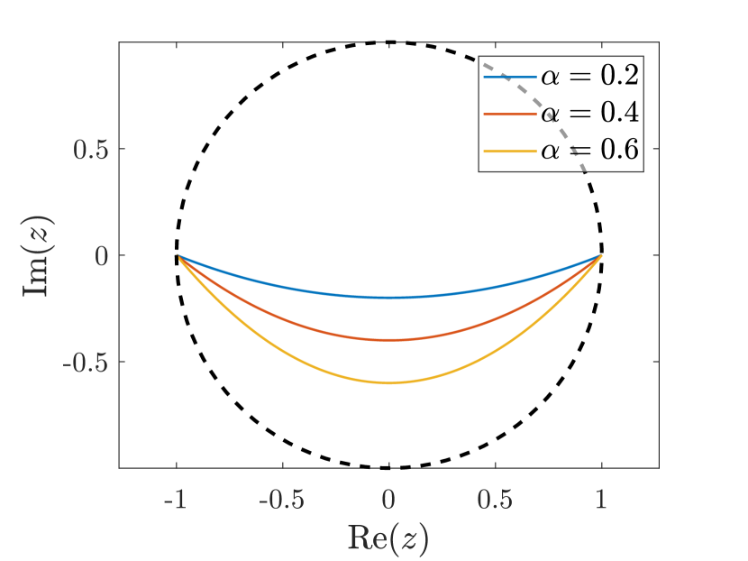
(a) $g(t)=t+i\alpha(t^{2}-1)$

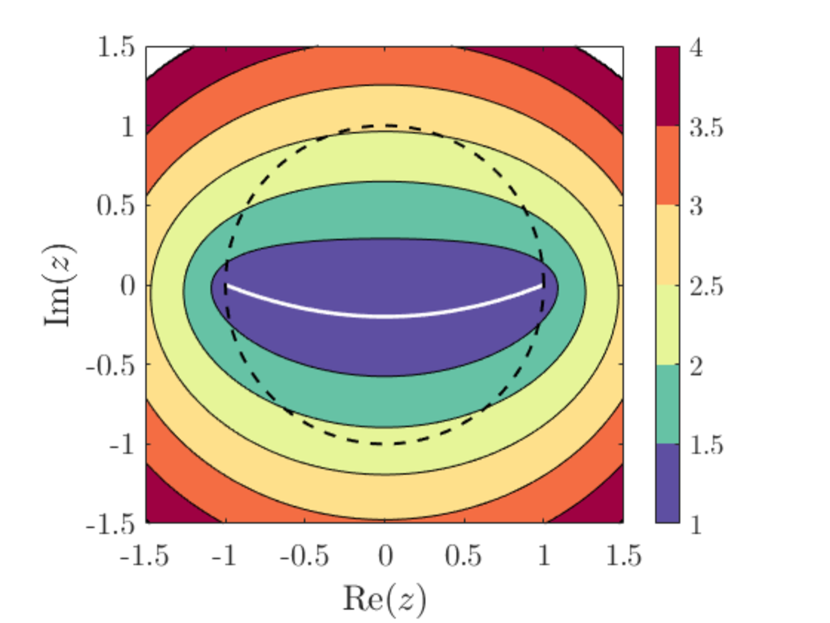
(b) $\alpha=0.2,\,\rho_{*}\approx 2.56$

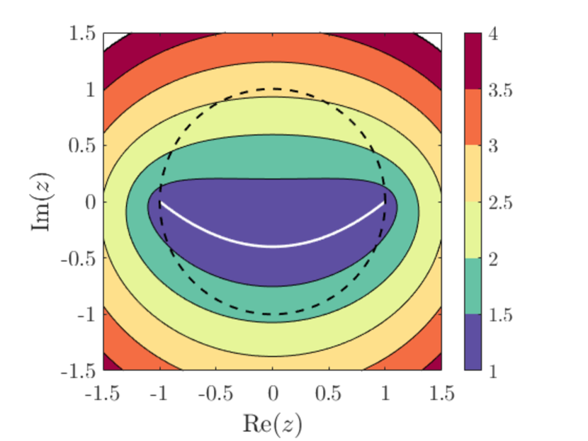
(c) $\alpha=0.4,\,\rho_{*}\approx 2.6$

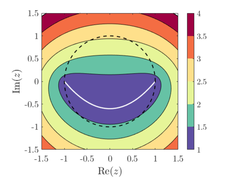
(d) $\alpha=0.6,\,\rho_{*}\approx 2.6$

Figure 13: The level set $E_{\rho}$ of a parabola, for various values of $\rho$. The colorbar indicates the value of $\rho$. The smooth simple arc $\Gamma$ is the white curve in the figure. The value of $\rho_{*}$ (see Definition 2.2) is estimated for each arc $\Gamma$.

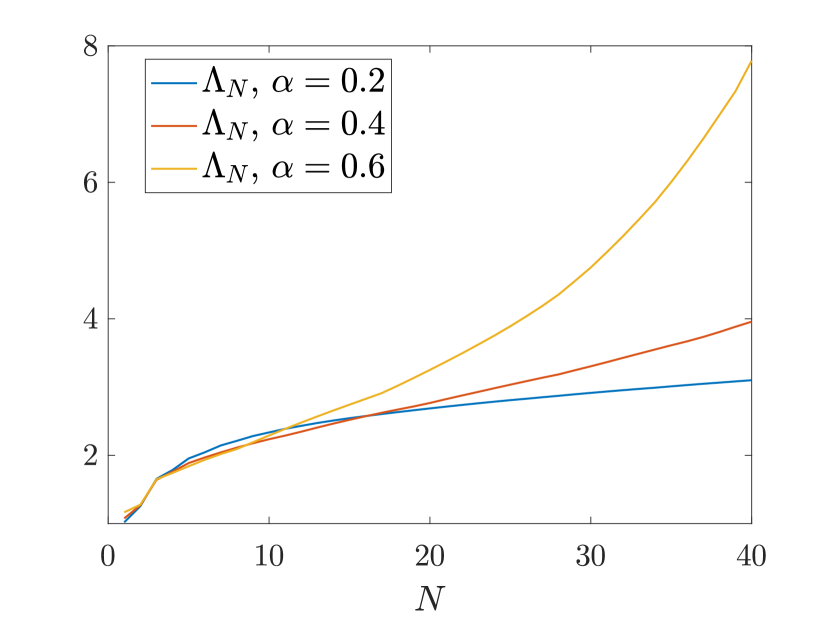
(a)

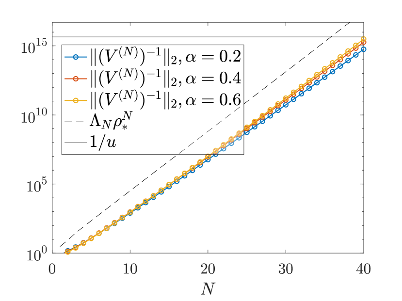
(b)

Figure 14: The Lebesgue constant for collocation points over a parabola, and the 2-norm of the inverse of the corresponding Vandermonde matrix. The collocation points are chosen to be $\{g(t_{j})\}$, where $\{t_{j}\}$ is a set of Chebyshev points over $[-1,1]$, and $g:[-1,1]\to\mathbbm{C}$ is the parameterization of the parabola defined in Section 2.4. The $x$-axis label $N$ denotes the order of approximation. The value of $\rho_{*}$ is set to be $2.6$, based on the estimate in Figure 13.

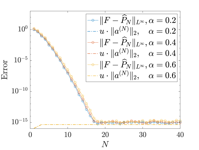
(a) $F(z)=\cos(2z+1)$

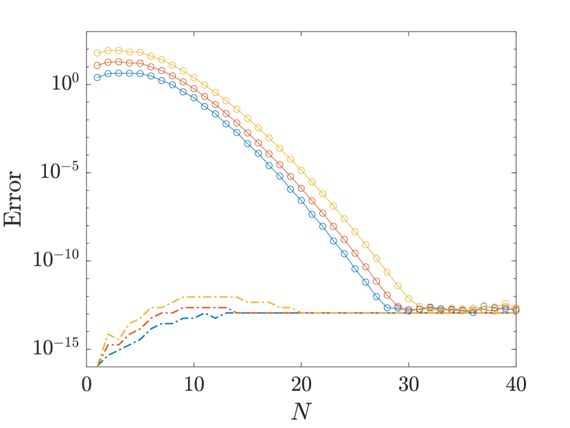
(b) $F(z)=\cos(8z+1)$

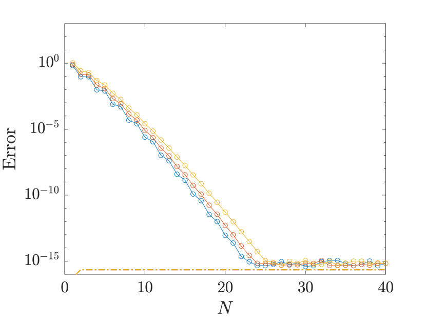
(c) $F(z)=e^{-z^{2}}$

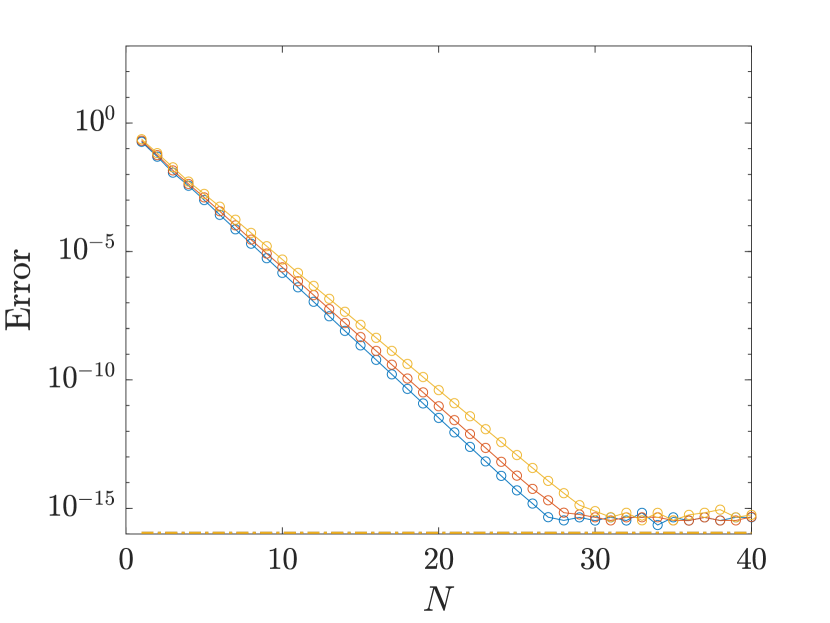
(d) $F(z)=\frac{1}{z-2}$

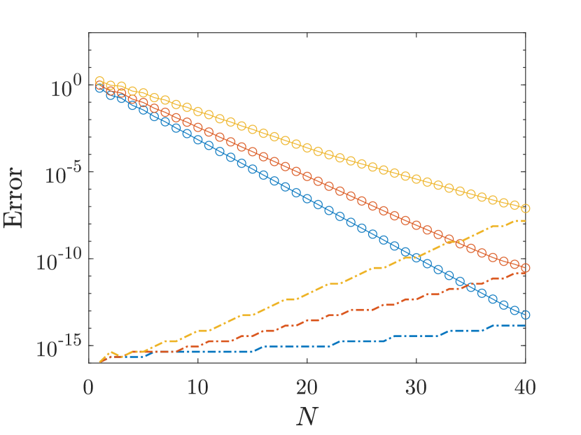
(e) $F(z)=\frac{1}{z+i}$

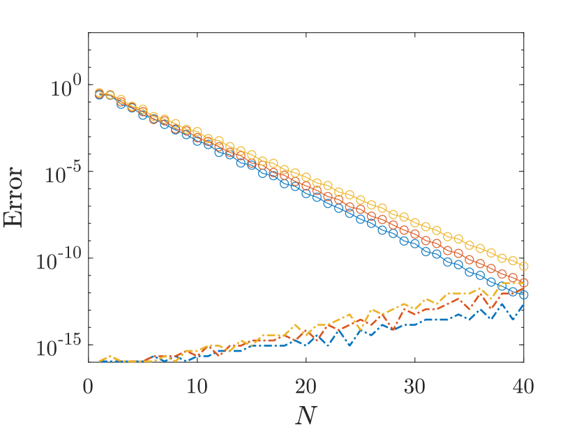
(f) $F(z)=\tan(\tan(z)/2)$

Figure 15: Polynomial interpolation in the monomial basis over a parabola. The interpolation is performed on the parabolas shown in Figure 13(a).

Remark 2.9.

In certain applications, the function $F:\Gamma\to\mathbbm{C}$ is defined by the formula $F(z):=\sigma(g^{-1}(z))$, where $g:[-1,1]\to\mathbbm{C}$ is an analytic function that parameterizes the curve $\Gamma$, and $\sigma:[-1,1]\to\mathbbm{C}$ is analytic. In this case, the analytic continuation of $F$ can have a singularity close to $\Gamma$ even when $\sigma$ is entire, because the inverse of the parameterization (i.e., $g^{-1}$) has so-called Schwarz singularities at $z=g(t^{*})$, where $g^{\prime}(t^{*})=0$. In [2], the authors show that, the higher the curvature of the arc $\Gamma$, the closer the singularity induced by $g^{-1}$ is to $\Gamma$. As a result, the approximation of such a function $F$ by polynomials is efficient only when the curvature of $\Gamma$ is small.

3 Applications

After justifying the use of a monomial basis for polynomial interpolation, a natural question to ask is: why would one want to do it in the first place? For one, the monomial basis is the simplest polynomial basis to manipulate. For example, the evaluation of an $N$th degree polynomial expressed in the monomial basis can be achieved using only $N$ multiplications through the application of Horner’s rule. This evaluation can be further accelerated using Estrin’s scheme, which has distinct advantages on modern processors. Additionally, the derivative and anti-derivative of an $N$th degree polynomial in the monomial basis can be calculated more stably in other bases, and using only $N$ multiplications. Besides these obvious advantages, we discuss some other applications below.

3.1 Oscillatory integrals and singular integrals

Given an oscillatory (or singular) function $\Psi:\Gamma\to\mathbbm{C}$ and a smooth function $F:\Gamma\to\mathbbm{C}$ over a smooth simple arc $\Gamma\subset\mathbbm{C}$, the calculation of $\int_{\Gamma}\Psi(z)F(z)\,\mathrm{d}z$ by standard quadrature rules can be extremely expensive or inaccurate due to the oscillations (or the singularity) of $\Psi$. However, when $F$ is a monomial, there exists a wide range of integrals in the form above that can be efficiently computed to high accuracy by either analytical formulas or by recurrence relations, often derived using integration by parts. Therefore, when the smooth function $F$ is accurately approximated by a monomial expansion of order $N$, such integrals can be efficiently evaluated by the formula $\sum_{k=0}^{N}a_{k}\Bigl{(}\int_{\Gamma}\Psi(z)z^{k}\,\mathrm{d}z\Bigr{)}$, where $\{a_{k}\}_{k=0,1,\dots,N}$ denotes the coefficients of the monomial expansion. Integrals of this type include the Fourier integral $\int_{a}^{b}e^{icx}F(x)\,\mathrm{d}x$, and various layer potentials, e.g., $\int_{\Gamma}\log(z-\xi)F(z)\,\mathrm{d}z$ and $\int_{\Gamma}\frac{F(z)}{z-\xi}\,\mathrm{d}z$, where $\xi\in\mathbbm{C}$ is given. We refer the readers to [20, 21] for more detailed discussion on the Fourier integral, and to [17, 2, 24] for more detailed discussion on the application of polynomial interpolation in the monomial basis to the evaluation of layer potentials. Some interesting applications can also be found in [18, 1, 22].

3.2 Root finding

Given a smooth simple arc $\Gamma\subset\mathbbm{C}$ and a function $F:\Gamma\to\mathbbm{C}$, one method for computing the roots of $F$ over $\Gamma$ is to first approximate it by a polynomial $P_{N}(z)=\sum_{j=0}^{N}a_{j}z^{j}$ to high accuracy, and then to compute the roots of $P_{N}$ by calculating the eigenvalues of the corresponding companion matrix. Recently, a backward stable algorithm that computes the eigenvalues of $C(P_{N})$ in $\mathcal{O}(N^{2})$ operations with $\mathcal{O}(N)$ storage has been proposed in [5]. This algorithm is backward stable in the sense that the computed roots are the exact roots of a perturbed polynomial $\widehat{P}_{N}(z)=\sum_{j=0}^{N}(a_{j}+\delta a_{j})z^{j}$, so that the backward error satisfies ${\lVert\delta a^{(N)}\rVert}_{2}\lesssim u{\lVert a^{(N)}\rVert}_{2}$, where $u$ denotes machine epsilon, $\delta a^{(N)}:=(\delta a_{0},\delta a_{1},\dots,\delta a_{N})^{T}$ and $a^{(N)}:=(a_{0},a_{1},\dots,a_{N})^{T}$. It follows that ${\lVert P_{N}-\widehat{P}_{N}\rVert}_{L^{\infty}(\Gamma)}\leq u{\lVert\delta a^{(N)}\rVert}_{1}\lesssim u\sqrt{N+1}{\lVert a^{(N)}\rVert}_{2}$. When ${\lVert a^{(N)}\rVert}_{2}\approx{\lVert P_{N}\rVert}_{L^{\infty}(\Gamma)}$, the computed roots are backward stable in the polynomial $P_{N}$. This condition, however, does not hold for all polynomials $P_{N}$. Furthermore, the calculation of the coefficients $a^{(N)}$ from the function $F$, which involves the solution of a Vandermonde system of equations, is highly ill-conditioned. In this paper, we show that, when $F$ is sufficiently smooth, it is possible to compute the coefficients of an interpolating polynomial $P_{N}(z)=\sum_{j=0}^{N}a_{j}z^{j}$, with ${\lVert a^{(N)}\rVert}_{2}\approx{\lVert F\rVert}_{L^{\infty}(\Gamma)}$, which approximates $F$ uniformly to high accuracy, even when the condition number of the Vandermonde matrix is close to the reciprocal of machine epsilon. From this, we see that a backward stable root finder can be constructed by combining the piecewise polynomial approximation procedure described in Section 2.2 with the algorithm presented in [5],

4 Discussion

Since the invention of digital computers, most research on the topic of polynomial interpolation in the monomial basis focuses on showing that it is a bad idea. The condition number of Vandermonde matrices has been studied extensively in recent decades (see [14] for a literature review), and it is known that its growth rate is at least exponential, unless the collocation nodes are distributed uniformly on the unit circle centered at the origin [23]. As a result, the computed monomial coefficients are generally highly inaccurate when the dimensionality of the Vandermonde matrix is not small. For this reason, other more well-conditioned bases are often used for polynomial interpolation [27, 11]. On the other hand, it has long been observed that polynomial interpolation in the monomial basis produces highly accurate approximations for sufficiently smooth functions (see, for example, [16, 17]). This is because that the inaccurately computed monomial coefficients does not imply that resulting interpolating polynomial is bad, since it is the backward error ${\lVert V\widehat{a}-f\rVert}_{2}$ of the numerical solution $\widehat{a}$ to the Vandermonde system $Va=f$ that determines the accuracy of the approximation, and ${\lVert V\widehat{a}-f\rVert}_{2}$ can be small even when the condition number $\kappa(V)$ is large. It has been shown in both frame approximations [3, 4] and the method of fundamental solutions [6, 26] that ${\lVert V\widehat{a}-f\rVert}_{2}\lesssim u\cdot{\lVert a\rVert}_{2}$, where $u$ denotes machine epsilon, from which it is easy to derive that the monomial approximation error is bounded by the sum of the polynomial interpolation error and the extra error term $u\cdot{\lVert a\rVert}_{2}$. In this paper, we characterize the growth of ${\lVert a\rVert}_{2}$, and show that this extra error term is generally smaller than the polynomial interpolation error, provided that the order of approximation is no larger than the maximum order allowed by the constraint $\kappa(V)\lesssim\frac{1}{u}$. Since this maximum order is not small in practice, we find that the monomial basis is a useful basis for interpolation, especially when it is used to construct a piecewise polynomial approximation.

While not discussed in this paper, our results can be easily generalized to higher dimensions. In [25], we study bivariate polynomial interpolation in the monomial basis over a (possibly curved) triangle, and demonstrate that the resulting order of approximation can reach up to 20, regardless of the triangle’s aspect ratio.

5 Acknowledgements

We are deeply grateful to James Bremer, Daan Huybrechs, Andreas Klöeckner, Adam Morgan, Nick Trefethen for their valuable advice and insightful discussions.

References

- [1] af Klinteberg, L., Askham, T., Kropinski, M. C.: A fast integral equation method for the two-dimensional Navier-Stokes equations. J. Comput. Phys., 409, 109353 (2020)
- [2] af Klinteberg, L., Barnett, A. H.: Accurate Quadrature of Nearly Singular Line Integrals in Two and Three Dimensions by Singularity Swapping. BIT Numer. Math. 61.1, 83–118 (2021)
- [3] Adcock, B., Huybrechs, D.: Frames and Numerical Approximation. SIAM Rev. 61(3), 443–473 (2019)
- [4] Adcock, B., Huybrechs, D.: Frames and Numerical Approximation II: Generalized Sampling. J. Fourier Anal. Appl. 26(6), 1–34 (2020)
- [5] Aurentz, J. L., Mach, T., Vandebril, R., Watkins, D. S.: Fast and Backward Stable Computation of Roots of Polynomials. SIAM J. Matrix Anal. Appl. 36(3), 942–973 (2015)
- [6] Barnett, A. H., Betcke, T.: Stability and Convergence of the Method of Fundamental Solutions for Helmholtz Problems on Analytic Domains. J. Comput. Phys. 227(14), 7003–7026 (2008)
- [7] Beckermann, B.: The Condition Number of Real Vandermonde, Krylov and Positive Definite Hankel Matrices. Numer. Math. 85(4), 553–577 (2000)
- [8] Berrut, J.-P., Trefethen, L. N.: Barycentric Lagrange Interpolation. SIAM Rev. 46(3), 501–517 (2004)
- [9] Björck, Å., Pereyra, V.: Solution of Vandermonde Systems of Equations. Math. Comput. 24(112), 893–903 (1970)
- [10] Börm, S.: On Iterated Interpolation. SIAM J. Numer. Anal. 60(6), 3124–3144 (2022)
- [11] Brubeck, P. D., Nakatsukasa Y., Trefethen, L. N.: Vandermonde with Arnoldi, SIAM Rev. 63(2), 405–415 (2021)
- [12] Ehlich, H., Zeller, K.: Auswertung der Normen von Interpolationsoperatoren. Math. Ann. 164, 105–112 (1966)
- [13] Estrada, R., Kanwal, R. P.: Singular Integral Equations. Springer Science & Business Media (2012)
- [14] Gautschi, W.: How (un)stable are Vandermonde systems?. Asymptot. Comput. Anal. 124, 193–210 (1990)
- [15] Gohberg, I., Olshevsky, V.: The Fast Generalized Parker–Traub Algorithm for Inversion of Vandermonde and Related Matrices. J. Complex. 13(2), 208–234 (1997)
- [16] Heath, M. T.: Scientific computing: an introductory survey, revised second edition. SIAM (2018)
- [17] Helsing, J., Ojala, R.: On the Evaluation of Layer Potentials Close to Their Sources. J. Comput. Phys. 227(5), 2899–2921 (2008)
- [18] Helsing, J., Jiang, S.: On Integral Equation Methods for the First Dirichlet Problem of the Biharmonic and Modified Biharmonic Equations in NonSmooth Domains. SIAM J. Sci. Comput. 40(4), A2609–2630 (2018)
- [19] Higham, N. J.: The Numerical Stability of Barycentric Lagrange Interpolation. IMA J. Numer. Anal. 24(4), 547–556 (2004)
- [20] Iserles, A., Nørsett, S. P.: Efficient Quadrature of Highly Oscillatory Integrals Using Derivatives. Proc. Math. Phys. Eng. 461(2057), 1383–1399 (2005)
- [21] Iserles, A., Nørsett, S. P., Olver, S.: Highly Oscillatory Quadrature: The Story So Far. In: Proceedings of ENumath, Santiago de Compostela (2006). Springer, Berlin, pp. 97–118 (2006)
- [22] Ojala, R., Tornberg, A.-K.: An Accurate Integral Equation Method for Simulating Multi-Phase Stokes Flow. J. Comp. Phys. 298, 145–160 (2015)
- [23] Pan, V. Y.: How bad are Vandermonde matrices?. SIAM J. Matrix Anal. Appl. 37(2), 676–694 (2016)
- [24] Wu, B., Zhu, H., Barnett, A., Veerapaneni S.: Solution of Stokes Flow in Complex Nonsmooth 2D Geometries via a Linear-Scaling High-Order Adaptive Integral Equation Scheme. J. Comput. Phys. 410, pp. 109361 (2020)
- [25] Shen, Z, Serkh, K.: Rapid evaluation of Newtonian potentials on planar domains. Accepted by SIAM J. Sci. Comput. arXiv:2208.10443 (2022)
- [26] Stein, D. B., Barnett, A. H.: Quadrature by Fundamental Solutions: Kernel-Independent Layer Potential Evaluation for Large Collections of Simple Objects. Adv. Comput. Math. 48(60) (2022)
- [27] Trefethen, L. N.: Approximation Theory and Approximation Practice. SIAM (2019)
- [28] Walsh, J. L.: Interpolation and Approximation by Rational Functions in the Complex Domain. vol. 20. AMS, Philadelphia (1935)
- [29] Zhong, L. F., Zhu, L. Y.: The Marcinkiewicz-Zygmund Inequality on a Smooth Simple Arc. J. Approx. Theory 83(1), 65–83 (1995)