Double Higgs production at NNLO interfaced to parton showers in GENEVA

Abstract

In this work, we study the production of Higgs boson pairs at next-to-next-to-leading order in QCD matched to parton showers, using the Geneva framework and working in the heavy-top-limit approximation. This includes the resummation of large logarithms of the zero-jettiness $\mathcal{T}_{0}$ up to the next-to-next-to-next-to-leading-log accuracy. This process features an extremely large momentum transfer, which makes its study particularly relevant for matching schemes such as that employed in Geneva, where the resummation of a variable different from that used in the ordering of the parton shower is used. To further study this effect, we extend the original shower interface designed for Pythia8 to include other parton showers, such as Dire and Sherpa.

1 Introduction

After the tenth anniversary of the Higgs boson discovery at the Large Hadron Collider (LHC) ATLAS:2012yve ; CMS:2012qbp , the study of its fundamental properties is still a very active field of research. Among all of the properties already measured – see for example Refs. ATLAS:2022tnm ; CMS:2022uhn and references therein – or in the processes to be measured CMS:2022wqf ; ATLAS:2022ers , one of the most important parameters connected with the electroweak symmetry breaking (EWSB) mechanism is the Higgs boson self-coupling, which, so far, has not yet been directly measured CMS:2022hgz ; CMS:2022kdx ; ATLAS:2022xzm ; ATLAS:2022hwc . Even with the future high-luminosity phase of the LHC, the Higgs self-coupling is only predicted to be constrained by around 50% DiMicco:2019ngk .

The measurement of the Higgs self-coupling is extremely dependent on precise theoretical predictions, and, at hadron colliders, it can be probed primarily through the production of a pair of Higgs bosons. Other indirect ways of estimating the self-coupling that exploit electroweak corrections in high precision observables have been proposed and studied Degrassi:2016wml ; Degrassi:2017ucl ; Maltoni:2017ims . Similar to the production of a single Higgs boson at hadron colliders, the main production mechanism of a Higgs pair is through a top-quark loop produced via gluon-gluon fusion Glover:1987nx . This means that already at the first non-trivial order in perturbation theory, one has to deal with a one-loop calculation Glover:1987nx ; Eboli:1987dy ; Plehn:1996wb , which makes the inclusion of higher-order terms particularly difficult. However, just as in the single Higgs boson case, one can treat the top quark as being infinitely heavy with respect to the Higgs boson, thus obtaining an effective gluon-gluon-Higgs vertex Glover:1987nx . Within this so-called heavy-top limit (HTL), the first results at next-to-leading-order (NLO) accuracy in QCD have been computed in Ref. Dawson:1998py , those at next-to-next-to-leading order (NNLO) in Refs. deFlorian:2013jea ; deFlorian:2016uhr , and at next-to-next-to-next-to-leading order (N³LO) in Refs. Chen:2019lzz ; Banerjee:2018lfq . Beyond the HTL, NLO results with full top-quark mass dependence have been presented in Refs. Borowka:2016ehy ; Borowka:2016ypz ; Baglio:2018lrj ; Baglio:2020ini . Approximations to include finite top-quark mass effects in fully differential calculations were discussed in Refs. Grazzini:2018bsd ; DeFlorian:2018eng up to the NNLO and in Ref. Chen:2019fhs at N³LO. Furthermore, the exact NLO results were combined with a resummation of logarithms of the transverse momentum of the Higgs pair system to next-to-leading logarithmic (NLL) accuracy Ferrera:2016prr , and a soft-gluon resummation to NLL was performed in Ref. DeFlorian:2018eng . Exact NLO results matched to the parton shower appeared in Refs. Heinrich:2017kxx ; Jones:2017giv ; Heinrich:2019bkc , while techniques to systematically include finite-mass effects had been studied Frederix:2014hta ; Maltoni:2014eza ; Maierhofer:2013sha before the exact NLO results became available. Several approaches towards analytical results for the two-loop amplitudes with full top-mass dependence based on different expansions were discussed in the literature Grigo:2013rya ; Grigo:2014jma ; Grigo:2015dia ; Degrassi:2016vss ; Grober:2017uho ; Bonciani:2018omm ; Davies:2018qvx ; Mishima:2018olh ; Davies:2019dfy ; Davies:2019djw ; Davies:2021kex ; Bellafronte:2022jmo .

In this work we provide the first implementation of the production of a Higgs pair at NNLO QCD in gluon-gluon fusion, using the HTL, matched to the parton shower. We do so using the well-established Geneva framework, which has been extensively exploited to provide fully differential results for various other colour singlet production processes Alioli:2015toa ; Alioli:2019qzz ; Alioli:2020fzf ; Alioli:2020qrd ; Alioli:2021egp ; Alioli:2021qbf . Our results feature the resummation of the zero-jettiness ($\mathcal{T}_{0}$) at next-to-next-to-leading-logarithmic accuracy within the primed counting (NNLL^′). While it is well known that the heavy-top approximation does not work as well for double Higgs production as it does for single Higgs boson Borowka:2016ehy ; Jones:2017giv ; Grazzini:2018bsd , the problem of including finite top-quark (and bottom-quark) mass effects is largely orthogonal to the problem of matching a NNLO calculation for $gg\to HH$ to the NNLL^′ resummation of $\mathcal{T}_{0}$ and to the parton shower. For this reason, in this work we neglect all power-like heavy-quark mass effects, but we note that for an accurate event generator these would have to be included. We leave the study of the inclusion of mass effects to a future publication. Note that other methods for the matching of NNLO calculations to the parton shower (NNLOPS in short) are available Hoche:2014dla ; Monni:2019whf ; Campbell:2021svd , but as far as we are aware no predictions for this specific process are available to date, using any of these methods.

The outline of this work is the following. First, in Sec. 2, we review the main features of the Geneva method, highlighting the differences with previous implementations which have been specifically designed for this process. Second, in Sec. 3, we validate our results by comparing to a fixed-order NNLO calculation provided by an independent code, Matrix Grazzini:2017mhc ; deFlorian:2016uhr . Next, in Sec. 4, we discuss the impact of the parton shower, presenting our results. Finally, in Sec. 5 we present our conclusions.

2 Theoretical framework

At hadron colliders, the production of a pair of Higgs bosons proceeds via two mechanisms. In the Standard Model (SM), at tree level, two Higgs bosons can be produced through heavy-quark (charm or bottom) annihilation through $s$- and $t$-channel diagrams Dawson:2006dm . At one-loop, one can instead produce a pair of Higgs bosons via a top-quark loop in triangle and box topologies in the gluon-gluon fusion channel. In the SM, the latter represents the dominant production mode, despite being suppressed by two powers of $\alpha_{S}$ compared to heavy-quark annihilation. This is due to the larger values of the gluon parton distribution function (PDF) at the relevant momentum transfer, combined with the larger coupling of the top quark to the Higgs boson. In the same spirit as the production of a single Higgs boson, to simplify the inclusion of higher-order effects, one can make the approximation that the top-quark mass is much larger than the hard scale of the process. This produces effective vertices directly coupling Higgs bosons and (two) gluons, and is normally referred to as HTL. We show in Fig. 1 the two leading-order (LO) diagrams contributing to this process in this approximation.

Figure 1: Leading-order diagrams for the production of a Higgs pair in the HTL.

It is important to stress that it is well known that the HTL is a much worse approximation in this particular case Borowka:2016ehy ; Jones:2017giv ; Grazzini:2018bsd compared to single Higgs boson production. There are two main causes for this. First, as this approximation receives corrections of the order $\mathcal{O}\left(Q^{2}/m_{t}^{2}\right)$, taking as a typical value for the momentum transfer $Q$ the peak of the invariant-mass distribution of the Higgs pair instead of the Higgs boson mass, we see that corrections are roughly three to four times larger for di-Higgs than for single Higgs production. Second, the two diagrams depicted in Fig. 1 arise from two different loop topologies: the triangle (left) and the box (right). While the latter is relatively well approximated in the HTL, the former is known, from the single scalar production case, to be a poor approximation for larger invariant masses of the $s$-channel particle. In this case, this is the mass of the virtual Higgs boson which can acquire extremely large values, thus spoiling the approximation. Moreover, in the exact result it is known that the interference between these two diagrams is large and negative, thus causing a large overall cancellation – this is not well-captured in the HTL.

In order to have a realistic event generator for this process, heavy-quark mass effects have to be included, and ways to include them order-by-order using approximants have been studied Davies:2019nhm . However, the present work is mainly concerned with the effects of matching the NNLO calculation for the FO production to the resummation of $\mathcal{T}_{0}$ and the subsequent matching to the parton shower, for this process. For these aspects, mass effects can be safely considered an orthogonal problem as they are not expected to considerably change the conclusions drawn in this paper. Lastly, due to the lack of available experimental data, for the time being we can safely ignore these effects. In the same spirit, when discussing the interface to the parton shower in Sec. 4, we also ignore all effects given by the hadronisation and fragmentation of hadrons in the shower, as well as those coming from multi-parton scattering.

In the rest of this section we recap the main features of the Geneva method, highlighting the main differences with respect to quark-induced processes that have been considered so far, and stressing the novelties developed during the completion of this work.

2.1 The Geneva method

Since the Geneva framework has already been extensively discussed in previous publications Alioli:2015toa ; Alioli:2019qzz ; Alioli:2020qrd ; Alioli:2021egp ; Alioli:2021qbf , for the sake of conciseness, we explicitly refrain from entering into the details of the method and only briefly recall the general formulae, highlighting some key features that are important for this process.

Geneva employs IR-safe resolution variables to discriminate between events, which are classified as having 0, 1 or 2 jets according to whether the value of a given resolution variable is smaller or larger than a given cutoff. Within this framework, from which the definition of “physical events” in a Monte Carlo generator naturally follows Alioli:2013hqa , unresolved emissions below the resolution cutoff are integrated over, and the IR safety of each event and at each perturbative order is ensured. For all the processes previously studied, a single cut in the resolution variable discriminating between zero or more jets, either on zero-jettiness $\mathcal{T}_{0}^{\mathrm{cut}}$ or on the transverse momentum of the colour singlet $q_{T}^{\mathrm{cut}}$, had always been used both for the resummed and the nonsingular components of the calculation. However, it is perfectly legitimate to move as much of the nonsingular contribution as possible into the resolved region of the phase space, such that it can be better described with the full event kinematics, while still maintaining the IR safety requirements. We recall that the variable $N$-jettiness Stewart:2010tn is defined as

$$\mathcal{T}_{N}=\sum_{k}\min\left[\hat{q}_{a}\cdot p_{k},\hat{q}_{b}\cdot p_{k},\hat{q}_{1}\cdot p_{k},...,\hat{q}_{N}\cdot p_{k}\right]\,,$$ (1)

with $N=0,1$, $\hat{q}_{a,b}$ are the beam directions and $\hat{q}_{k}$ represents any final-state massless four-vector that minimises $\mathcal{T}_{N}$, and $p_{k}$ are the momenta of the final-state partons. Therefore, in the following we explicitly use 0-jettiness as our main resolution variable and consider two separate cuts: $\mathcal{T}_{0,\rm re}^{\mathrm{cut}}$ acting on the resummed singular contribution and $\mathcal{T}_{0,\rm ns}^{\mathrm{cut}}$ acting on the nonsingular. These effectively replace the common $\mathcal{T}_{0}^{\mathrm{cut}}$ used in previous Geneva implementations. Choosing $\mathcal{T}_{0,\rm ns}^{\mathrm{cut}}$ smaller than $\mathcal{T}_{0,\rm re}^{\mathrm{cut}}$ allows us to push down the calculation of the nonsingular contributions to lower values, thereby reducing the subleading power corrections. Note, however, that the result should be independent of the exact choice of $\mathcal{T}_{0,\rm re}^{\mathrm{cut}}$, modulo higher-order corrections.

With these definitions, the differential cross sections for the production of events with $0,1$, and $\geq 2$ emissions are given by

$$\frac{\mathrm{d}\sigma^{\textsc{mc}}_{0}}{\mathrm{d}\Phi_{0}}(\mathcal{T}_{0,\rm re}^{\mathrm{cut}},\mathcal{T}_{0,\rm ns}^{\mathrm{cut}}) =\frac{\mathrm{d}\sigma^{\rm NNLL^{\prime}}}{\mathrm{d}\Phi_{0}}(\mathcal{T}_{0,\rm re}^{\mathrm{cut}})-\frac{\mathrm{d}\sigma^{\rm NNLL^{\prime}}}{\mathrm{d}\Phi_{0}}(\mathcal{T}_{0,\rm ns}^{\mathrm{cut}})\bigg{|}_{\mathrm{NNLO}_{0}}$$

$$\qquad+(B_{0}+V_{0}+W_{0})(\Phi_{0})\,+\,\int\frac{\mathrm{d}\Phi_{1}}{\mathrm{d}\Phi_{0}}(B_{1}+V_{1})(\Phi_{1})\,\theta\big{(}\mathcal{T}_{0}(\Phi_{1})<\mathcal{T}_{0,\rm ns}^{\mathrm{cut}}\big{)}$$

$$\qquad+\int\frac{\mathrm{d}\Phi_{2}}{\mathrm{d}\Phi_{0}}\,B_{2}(\Phi_{2})\,\theta\big{(}\mathcal{T}_{0}(\Phi_{2})<\mathcal{T}_{0,\rm ns}^{\mathrm{cut}}\big{)}\,,$$ (2)

$$\frac{\mathrm{d}\sigma^{\textsc{mc}}_{1}}{\mathrm{d}\Phi_{1}} (\mathcal{T}_{0}>\mathcal{T}_{0,\rm ns}^{\mathrm{cut}};\mathcal{T}_{0,\rm re}^{\mathrm{cut}};\mathcal{T}_{1}^{\mathrm{cut}})=\Bigg{\{}\frac{\mathrm{d}\sigma^{\rm NNLL^{\prime}}}{\mathrm{d}\Phi_{0}\mathrm{d}\mathcal{T}_{0}}\mathcal{P}(\Phi_{1})\,\theta(\mathcal{T}_{0}>\mathcal{T}_{0,\rm re}^{\mathrm{cut}})$$ (3)

$$+\bigg{[}(B_{1}+V_{1}^{C})(\Phi_{1})-\frac{\mathrm{d}\sigma^{\rm NNLL^{\prime}}}{\mathrm{d}\Phi_{0}\mathrm{d}\mathcal{T}_{0}}\bigg{|}_{\mathrm{NLO}_{1}}\mathcal{P}(\Phi_{1})\bigg{]}\theta(\mathcal{T}_{0}>\mathcal{T}_{0,\rm ns}^{\mathrm{cut}})\Bigg{\}}\times\,U_{1}(\Phi_{1},\mathcal{T}_{1}^{\mathrm{cut}})$$

$$+\int\ \bigg{[}\frac{\mathrm{d}\Phi_{2}}{\mathrm{d}\Phi^{\mathcal{T}}_{1}}\,B_{2}(\Phi_{2})\,\theta\!\left(\mathcal{T}_{0}(\Phi_{2})>\mathcal{T}_{0,\rm ns}^{\mathrm{cut}}\right)\,\theta(\mathcal{T}_{1}<\mathcal{T}_{1}^{\mathrm{cut}})-\frac{\mathrm{d}\Phi_{2}}{\mathrm{d}\Phi^{C}_{1}}\,C_{2}(\Phi_{2})\,\theta(\mathcal{T}_{0}>\mathcal{T}_{0,\rm ns}^{\mathrm{cut}})\bigg{]}$$

$$-B_{1}(\Phi_{1})\,U_{1}^{({1})}(\Phi_{1},\mathcal{T}_{1}^{\mathrm{cut}})\,\theta(\mathcal{T}_{0}>\mathcal{T}_{0,\rm ns}^{\mathrm{cut}})\,,$$

$$\frac{\mathrm{d}\sigma^{\textsc{mc}}_{\geq 2}}{\mathrm{d}\Phi_{2}} (\mathcal{T}_{0}>\mathcal{T}_{0,\rm ns}^{\mathrm{cut}};\mathcal{T}_{0,\rm re}^{\mathrm{cut}};\mathcal{T}_{1}>\mathcal{T}_{1}^{\mathrm{cut}})=$$ (4)

$$\Bigg{\{}\Bigg{[}(B_{1}+V_{1}^{C})({\Phi}_{1})-\frac{\mathrm{d}\sigma^{\rm NNLL^{\prime}}}{\mathrm{d}\Phi_{0}\mathrm{d}\mathcal{T}_{0}}\bigg{|}_{\mathrm{NLO}_{1}}\mathcal{P}({\Phi}_{1})\Bigg{]}\theta(\mathcal{T}_{0}>\mathcal{T}_{0,\rm ns}^{\mathrm{cut}})\Big{|}_{{\Phi}_{1}=\Phi_{1}^{\mathcal{T}}\!(\Phi_{2})}\bigg{]}$$

$$+\frac{\mathrm{d}\sigma^{\rm NNLL^{\prime}}}{\mathrm{d}\Phi_{0}\mathrm{d}\mathcal{T}_{0}}\,\mathcal{P}({\Phi}_{1})\,\theta(\mathcal{T}_{0}>\mathcal{T}_{0,\rm re}^{\mathrm{cut}})\Big{|}_{{\Phi}_{1}=\Phi_{1}^{\mathcal{T}}\!(\Phi_{2})}\Bigg{\}}\,U_{1}^{\prime}({\Phi}_{1},\mathcal{T}_{1})\,\mathcal{P}(\Phi_{2})\,\theta(\mathcal{T}_{1}>\mathcal{T}_{1}^{\mathrm{cut}})$$

$$+B_{2}(\Phi_{2})\,\theta(\mathcal{T}_{1}>\mathcal{T}^{\mathrm{cut}}_{1})\theta\left(\mathcal{T}_{0}(\Phi_{2})>\mathcal{T}_{0,\rm ns}^{\mathrm{cut}}\right)\,$$

$$-B_{1}(\Phi_{1}^{\mathcal{T}})\,U_{1}^{({1})\prime}\big{(}{\Phi}_{1},\mathcal{T}_{1}\big{)}\,\mathcal{P}(\Phi_{2})\,\Theta(\mathcal{T}_{1}>\mathcal{T}_{1}^{\mathrm{cut}})\,\theta\left(\mathcal{T}_{0}(\Phi_{2})>\mathcal{T}_{0,\rm ns}^{\mathrm{cut}}\right)\,.$$

In the previous formulae $B_{0,1,2}$ represents the $0,1,2$-parton tree-level contributions, $V_{0,1}$ the $0,1$-parton one-loop contributions and $W_{0}$ the two-loop contributions. We have introduced the notation

$$\frac{\mathrm{d}\Phi_{M}}{\mathrm{d}\Phi_{N}^{\mathcal{T}}}=\mathrm{d}\,\Phi_{M}\delta[\Phi_{N}-\Phi_{N}^{\mathcal{T}}(\Phi_{M})]\,\Theta^{\mathcal{T}}(\Phi_{M}),\qquad N\leq M\,,$$ (5)

to indicate that the integration over a region of the $M$-body phase space is done keeping the $N$-body phase space and the value of the observable $\mathcal{T}$ fixed. The $\Theta^{\mathcal{T}}(\Phi_{N})$ term limits the integration region to the phase space points included in the singular contribution for the observable $\cal{T}$. The $V_{1}^{C}$ term includes contributions of soft and collinear origin and it is defined as

$$V_{1}^{C}(\Phi_{1})=V_{1}(\Phi_{1})+\int\frac{\mathrm{d}\Phi_{2}}{\mathrm{d}\Phi_{1}^{C}}\,C_{2}(\Phi_{2})\,,$$ (6)

where $C_{2}$ acts as a local NLO subtraction counterterm that reproduces the singular behaviour of $B_{2}$. The subtraction counterterms are integrated over the radiation variables $\frac{\mathrm{d}\Phi_{2}}{\mathrm{d}\Phi_{1}^{C}}$ considering the singular limit $C$ of the phase space mapping.
We have also introduced normalised splitting functions $\mathcal{P}(\Phi_{N+1})$ to make the resummed $\mathcal{T}_{N}$ spectrum fully differential in $\Phi_{N+1}$. These splitting functions are normalised such that

$$\int\mathcal{P}(\Phi_{N+1})\,\frac{\mathrm{d}\Phi_{N+1}}{\mathrm{d}\Phi_{N}\,\mathrm{d}\mathcal{T}_{N}}=1,$$ (7)

where two extra emission variables, the energy ratio $z$ and the azimuthal angle $\phi$, are needed besides $\mathcal{T}_{N}$ to define a splitting $\Phi_{N}\to\Phi_{N+1}$. The normalised splitting probability is given by

$$\small{\mathcal{P}\!\left(\Phi_{N+1}\right)=\frac{\displaystyle f_{kj}\!\left(\Phi_{N},\mathcal{T}_{N},z\right)}{\displaystyle\sum_{k^{\prime}=1}^{N+2}\int_{z_{\mathchoice{\displaystyle}{\displaystyle}{\scriptscriptstyle}{\scriptscriptstyle}\rm min}^{k^{\prime}}\!\left(\Phi_{N},\mathcal{T}_{N}\right)}^{z_{\mathchoice{\displaystyle}{\displaystyle}{\scriptscriptstyle}{\scriptscriptstyle}\rm max}^{k^{\prime}}\!\left(\Phi_{N},\mathcal{T}_{N}\right)}\mathrm{d}z^{\prime}\,J_{k^{\prime}}\!\left(\Phi_{N},\mathcal{T}_{N},z^{\prime}\right)I_{\phi}^{k^{\prime}}\!\left(\Phi_{N},\mathcal{T}_{N},z^{\prime}\right)\sum_{j^{\prime}=1}^{n_{\rm split}^{k^{\prime}}}f_{k^{\prime}j^{\prime}}\!\left(\Phi_{N},\mathcal{T}_{N},z^{\prime}\right)}}\,,$$ (8)

where

$$I_{\phi}^{k}\!\left(\Phi_{N},\mathcal{T}_{N},z\right)=\phi_{\mathchoice{\displaystyle}{\displaystyle}{\scriptscriptstyle}{\scriptscriptstyle}\rm max}^{k}\!\left(\Phi_{N},\mathcal{T}_{N},z\right)-\phi_{\mathchoice{\displaystyle}{\displaystyle}{\scriptscriptstyle}{\scriptscriptstyle}\rm min}^{k}\!\left(\Phi_{N},\mathcal{T}_{N},z\right).$$ (9)

In the formula above $f_{kj}\left(\Phi_{N},\mathcal{T}_{N},z\right)$ are generic functions based on the Altarelli-Parisi splitting functions, $z_{{\mathchoice{\displaystyle}{\displaystyle}{\scriptscriptstyle}{\scriptscriptstyle}\rm min},{\mathchoice{\displaystyle}{\displaystyle}{\scriptscriptstyle}{\scriptscriptstyle}\rm max}}(\Phi_{N},\mathcal{T}_{N},z)$, $\phi_{{\mathchoice{\displaystyle}{\displaystyle}{\scriptscriptstyle}{\scriptscriptstyle}\rm min},{\mathchoice{\displaystyle}{\displaystyle}{\scriptscriptstyle}{\scriptscriptstyle}\rm max}}(\Phi_{N},\mathcal{T}_{N},z)$ are the integration limits, respectively, in $z$ and $\phi$ defined in Ref. Gavardi:2023oho , and $J\left(\Phi_{N},\mathcal{T}_{N},z\right)$ is the Jacobian related to the change of variable. Further details about this new implementation of the splitting probabilities are discussed in a separate publication Alioli:2023har .

In equations (3) and (4) we introduce the Sudakov factor $U_{1}(\Phi_{1},\mathcal{T}^{\mathrm{cut}}_{1})$ which resums the dependence of $\mathcal{T}^{\mathrm{cut}}_{1}$ to next-to-leading-logarithmic (NLL) accuracy. In addition to the formulae for the quark channels already presented in Ref. Alioli:2016wqt , for gluon-initiated processes we have

$$U^{ggg}_{1}(\Phi_{1},\mathcal{T}^{\mathrm{cut}}_{1})=\frac{U}{\Gamma\bigg{(}1+6\,C_{A}\,\eta^{\rm NLL}_{\rm cusp}(\mu_{S},\mu_{H})\bigg{)}}\,,$$ (10)

with $\Gamma$ the Euler gamma function and

$$\ln U =6\,C_{A}\bigg{[}2\,K^{\rm NLL}_{\Gamma_{\rm cusp}}(\mu_{J},\mu_{H})-K^{\rm NLL}_{\Gamma_{\rm cusp}}(\mu_{S},\mu_{H})\bigg{]}$$

$$+C_{A}\bigg{[}-\ln\bigg{(}\frac{Q^{2}_{a}Q^{2}_{b}Q^{2}_{J}}{\mu^{6}_{H}}\bigg{)}\,\eta^{\rm NLL}_{\Gamma_{\rm cusp}}(\mu_{J},\mu_{H})+\ln\bigg{(}\frac{Q^{2}_{a}Q^{2}_{b}Q^{2}_{J}}{stu}\bigg{)}\,\eta^{\rm NLL}_{\Gamma_{\rm cusp}}(\mu_{S},\mu_{H})\bigg{]}$$

$$-6\,\gamma_{E}\,C_{A}\,\eta^{\rm NLL}_{\Gamma_{\rm cusp}}(\mu_{S},\mu_{J})+3\,K^{\rm NLL}_{\gamma^{g}_{J}}(\mu_{J},\mu_{H}).$$ (11)

The functions appearing in the formula above are common in the SCET literature, see e.g. Ref. Berger:2010xi , and are given by

$$K^{\rm NLL}_{\Gamma_{\rm cusp}}(\mu_{1},\mu_{2}) =-\frac{\Gamma_{0}}{4\beta^{2}_{0}}\bigg{[}\frac{4\pi}{\alpha_{S}(\mu_{1})}\bigg{(}1-\frac{1}{r}-\ln r\bigg{)}+\bigg{(}\frac{\Gamma_{1}}{\Gamma_{0}}-\frac{\beta_{1}}{\beta_{0}}\bigg{)}(1-r\ln r)+\frac{1}{2}\frac{\beta_{1}}{\beta_{0}}\ln^{2}r\bigg{]},$$

$$\eta^{\rm NLL}_{\Gamma_{\rm cusp}}(\mu_{1},\mu_{2}) =-\frac{1}{2}\frac{\Gamma_{0}}{\beta_{0}}\bigg{[}\ln r+\frac{\alpha_{S}(\mu_{1})}{4\pi}\bigg{(}\frac{\Gamma_{1}}{\Gamma_{0}}-\frac{\beta_{1}}{\beta_{0}}\bigg{)}(r-1)\bigg{]},$$

$$K^{\rm NLL}_{\gamma_{J}} =-\frac{1}{2}\frac{\gamma_{0}}{\beta_{0}}\ln r\,,$$ (12)

with $r=\frac{\alpha_{S}(\mu_{2})}{\alpha_{S}(\mu_{1})}$, the scales $\mu_{H}=\mathcal{T}_{1}^{\max}$, $\mu_{S}=\mathcal{T}_{1}^{\mathrm{cut}}$ and $\mu_{J}=\sqrt{\mu_{H}\mu_{S}}$. The kinematics-dependent terms are given by

$$Q_{a}=p_{a}\,Q_{HH}\,e^{Y_{HH}},\qquad Q_{b}=p_{b}\,Q_{HH}\,e^{-Y_{HH}},\qquad Q_{J}=2\,p_{J}\,E_{J}\,,$$ (13)

where $Q_{HH}$ is the invariant mass of the di-Higgs system, $Y_{HH}$ its rapidity, $p_{a,b}$ are the incoming momenta, $p_{J}$ is the momentum and $E_{J}$ the energy of the jet in the final state (in the frame in which the Higgs pair system has $Y_{HH}=0$). The cusp and noncusp anomalous dimensions are given by

$$\Gamma_{0}=4\,,\qquad\Gamma_{1}=4\bigg{[}\bigg{(}\frac{67}{9}-\frac{\pi^{2}}{3}\bigg{)}C_{A}-\frac{20}{9}T_{F}n_{f}\bigg{]}\,,$$

$$\gamma_{0}=12C_{F}+2\beta_{0}\,,\qquad\beta_{0}=\frac{11}{3}C_{A}-\frac{4}{3}T_{F}n_{f}\,,$$

$$\beta_{1}=\frac{34}{3}C^{2}_{A}-\frac{10}{3}C_{A}n_{f}-2C_{F}n_{f}\,.$$ (14)

With $U_{1}^{\prime}$ we denote the first derivative of $U_{1}(\Phi_{1},\mathcal{T}_{1})$ with respect to $\mathcal{T}_{1}$, and with $U^{\prime(1)}_{1}$ and $U^{(1)}_{1}$ their $\mathcal{O}(\alpha_{S})$ expansions, respectively.

All the non-projectable regions of $\Phi_{1}$ and $\Phi_{2}$, due to events that e.g. result in an invalid flavour projection or come from points in the phase space not covered by the $\mathcal{T}_{0}$-preserving mapping, are included in the event samples with $1$ or $2$ additional emissions below the resolution cutoffs. We assign them the following cross sections,

$$\frac{\mathrm{d}\sigma^{\textsc{mc}}_{1}}{\mathrm{d}\Phi_{1}}(\mathcal{T}_{0}\leq\mathcal{T}_{0,\rm ns}^{\mathrm{cut}};\mathcal{T}_{1}^{\mathrm{cut}}) =(B_{1}+V_{1})(\Phi_{1})\,\overline{\Theta}^{\mathrm{FKS}}_{\mathrm{map}}(\Phi_{1})\,\theta(\mathcal{T}_{0}<\mathcal{T}_{0,\rm ns}^{\mathrm{cut}})\,,$$ (15)

$$\frac{\mathrm{d}\sigma^{\textsc{mc}}_{\geq 2}}{\mathrm{d}\Phi_{2}}(\mathcal{T}_{0}>\mathcal{T}_{0,\rm ns}^{\mathrm{cut}};\mathcal{T}_{1}\leq\mathcal{T}_{1}^{\mathrm{cut}}) =B_{2}(\Phi_{2})\,\overline{\Theta}_{\mathrm{map}}^{\mathcal{T}}(\Phi_{2})\,\theta(\mathcal{T}_{1}<\mathcal{T}_{1}^{\mathrm{cut}})\,\theta\left(\mathcal{T}_{0}(\Phi_{2})>\mathcal{T}_{0,\rm ns}^{\mathrm{cut}}\right)\,.$$ (16)

The quantity $\Theta^{\mathrm{X}}_{\mathrm{map}}$ encodes the constraints due to the projections in the two mappings: the FKS map in the case of the $\Phi_{1}\to{\Phi}_{0}$ projection and the $\mathcal{T}_{0}$-preserving map for the $\Phi_{2}\to{\Phi}_{1}$ projection. The overlined versions represent their complements.

2.2 $\mathcal{T}_{0}$ resummation

In order to compute our results in the region below $\mathcal{T}_{0}^{\mathrm{cut}}$, as well as to perform the $\mathcal{T}_{0}$ resummation, we rely on the factorisation theorem for the zero-jettiness in the SCET formalism. For the particular case at hand, it means that we can write the factorised differential cross section as Stewart:2009yx

$$\frac{\mathrm{d}\sigma^{\rm SCET}}{\mathrm{d}\Phi_{0}\,\mathrm{d}\mathcal{T}_{0}}=H_{{\scriptscriptstyle gg\to HH}}(Q^{2},\mu)\int B_{g}(t_{a},x_{a},\mu)\,B_{g}(t_{b},x_{b},\mu)\,S_{gg}\left(\mathcal{T}_{0}-\frac{t_{a}+t_{b}}{Q},\mu\right)\,\mathrm{d}t_{a}\,\mathrm{d}t_{b}.$$ (17)

In the above formula $H_{{\scriptscriptstyle gg\to HH}}$ is the hard function, $B_{g}$ the beam function and $S_{gg}$ the soft function. The hard function is process dependent and contains the corresponding Born and virtual matrix elements. The soft function depends on the external partons in the process: for colour singlet production in the gluon fusion channel, its perturbative component is derived from that calculated for the quark channels through Casimir rescaling. Similarly, the beam functions also depend on whether the process is quark- or gluon-initiated. They depend on the transverse virtualities $t_{a,b}$, and for $t_{a,b}\gg\Lambda_{\textrm{QCD}}$ they satisfy an operator product expansion (OPE) in terms of perturbative collinear matching coefficients and standard parton distribution functions.

Each of these three functions admits a perturbative expansion in powers of the strong coupling and manifests a logarithmic dependence on a single characteristic scale. The canonical choice of scales that minimises these logarithmic terms is

$$\mu_{H}=Q,\qquad\mu_{B}=\sqrt{Q\mathcal{T}_{0}},\qquad\mu_{S}=\mathcal{T}_{0}.$$ (18)

Provided this choice of scales is made, there are no leftover large logarithms in the perturbative expansion of $H$, $B$ and $S$. However, the factorisation formula requires all the components to be evaluated at a single common scale $\mu$. This is achieved by acting with the renormalisation group evolution (RGE) operator on each function, which results in the following schematic representation of the resummed $\mathcal{T}_{0}$ spectrum,

$$\frac{\mathrm{d}\sigma^{\rm NNLL^{\prime}}}{\mathrm{d}\Phi_{0}\mathrm{d}\mathcal{T}_{0}}= H_{{\scriptscriptstyle gg\to HH}}(Q^{2},\mu_{H})\,U_{H}(\mu_{H},\mu)$$

$$\times\int\mathrm{d}t_{a}\,\mathrm{d}t_{b}\left[B_{g}(t_{a},x_{a},\mu_{B})\otimes U_{B}(\mu_{B},\mu)\right]\left[B_{g}(t_{b},x_{b},\mu_{B})\otimes U_{B}(\mu_{B},\mu)\right]$$

$$\qquad\times\left[S_{gg}(\mathcal{T}_{0}-\frac{t_{a}+t_{b}}{Q},\mu_{S})\otimes U_{S}(\mu_{S},\mu)\right],$$ (19)

where we abbreviated the convolution over internal variables using the symbol $\otimes$. In the formula above the large logarithms arising from ratios of disparate scales in Eq. (17) have been resummed by the RGE factors $U_{i}(\mu_{i},\mu)$.

At NNLL^′ accuracy the anomalous dimensions appearing in the evolution factors need to be known at 2- and 3-loop order for the noncusp Berger:2010xi and cusp terms Moch:2004pa ; Vogt:2004mw ; Korchemsky:1987wg , respectively. Similarly, the QCD beta function Tarasov:1980au ; Larin:1993tp is required to be known at 3-loop order. In addition, the hard, beam and soft functions have to be computed at 2-loop order. The necessary soft function has been computed at 2-loops in Refs. Kelley:2011ng ; Monni:2011gb . The hard function is taken from Refs. deFlorian:2013uza and Grigo:2014jma , translating the result from the Catani scheme to the $\overline{\rm MS}$ scheme, which we use in Geneva. The details of this calculation can be found in Appendix A. Finally, the beam functions are known up to 3-loops Gaunt:2014cfa ; Ebert:2020unb .

In order to extend the resummation accuracy of Geneva to N³LL, the noncusp and cusp anomalous dimensions Berger:2010xi ; vanRitbergen:1997va ; vonManteuffel:2020vjv , the QCD beta function vanRitbergen:1997va and the running of the strong coupling have to be included at one order higher.

2.2.1 Choice of scales and their impact on observables

In this section we describe the procedure we use to set all the scales entering both the FO and the resummed parts of our calculation. To be able to smoothly match the regions where the logarithms of $\tau=\mathcal{T}_{0}/Q$ are large and where they are sub-dominant, we need to turn off the resummation around a value of $\mathcal{T}_{0}\sim Q$, for some hard scale $Q$. We choose $Q$ to be equal to the FO scale, which in turn equals the invariant mass of the Higgs boson pair, $M_{HH}$. For larger values of $\mathcal{T}_{0}$, since the cross section is well approximated by the FO result, it is important to switch off the resummation as $\mathcal{T}_{0}\to Q$. Failing to do so would spoil the cancellation between the singular and the nonsingular terms. In the SCET approach, where the resummation is carried out via RGE, this can be achieved by evolving the soft and beam functions to the same common nonsingular scale $\mu_{\rm NS}=M_{HH}$ as that of the hard function, which is always computed at $\mu_{\rm NS}$. The evolution of the soft and beam functions is done by using profile scales $\mu_{S}(\mathcal{T}_{0})$ and $\mu_{B}(\mathcal{T}_{0})$. These conventions have been introduced in Ref. Berger:2010xi , and are given by

$$\mu_{S}(\mathcal{T}_{0}) =\mu_{\rm NS}\,f_{\rm run}(\mathcal{T}_{0}/Q),$$

$$\mu_{B}(\mathcal{T}_{0}) =\mu_{\rm NS}\,\sqrt{f_{\rm run}(\mathcal{T}_{0}/Q)},$$ (20)

where $f_{\rm run}$ is defined as

$$f_{\rm run}(x)=\begin{cases}x_{0}[1+(x/(2x_{0}))^{2}]&x\leq 2x_{0},\\ x&2x_{0}<x\leq x_{1},\\ x+\frac{(2-x_{1}-x_{2})(x-x_{1})^{2}}{2(x_{2}-x_{1})(x_{3}-x_{1})}&x_{1}<x\leq x_{2},\\ 1-\frac{(2-x_{1}-x_{2})(x-x_{3})^{2}}{2(x_{3}-x_{1})(x_{3}-x_{2})}&x_{2}<x\leq x_{3},\\ 1&x_{3}<x.\end{cases}$$ (21)

This functional form ensures the canonical scaling, given by Eq. (18), between $x_{0}$ and $x_{1}$ and switches off the resummation above $x_{3}$. The region below $2\,x_{0}$ corresponds to the region where we freeze the running of all couplings to avoid the Landau pole. The point $x_{2}$ corresponds to an inflection point in the profile function $f_{\rm run}$. In Fig. 2 we compare the absolute sizes of the singular and nonsingular contributions to the cross section as functions of $\tau$ at $\rm LO_{1}$ and $\rm NLO_{1}$ accuracy, where LO₁ and NLO₁ refer to the order relative to the partonic phase space with one extra emission. By default we set the profile parameters to

$$x_{0}=\frac{1\,\,\mathrm{GeV}}{Q},\qquad\{x_{1},x_{2},x_{3}\}=\{0.2,0.275,0.35\}.$$ (22)

The values of $x_{1}$ and $x_{3}$ are chosen at the points where FO and singular contributions are of similar size and where the nonsingular contribution becomes dominant, respectively.

We obtain theoretical uncertainties for the FO prediction by varying the central scale $\mu_{\rm NS}$ up and down by a factor of two and taking the maximal absolute deviation from the central value as a measure of uncertainty. For the resummed case we vary the central choices for the profile scales $\mu_{S}$ and $\mu_{B}$ independently, as e.g. detailed in Alioli:2019qzz , keeping $\mu_{H}=\mu_{\rm NS}$ fixed. We include also two more profiles where all the $x_{i}$ are varied by $\pm 0.05$ simultaneously, while keeping all the other scales at their central values. In total we get six profile variations and take the maximal absolute deviation in the result from the central value as the resummation uncertainty. The total uncertainty is then given by the quadrature sum of the resummation and FO uncertainties.

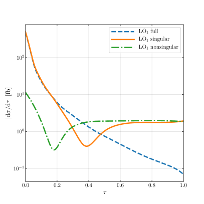
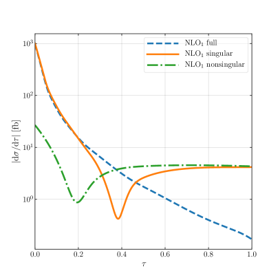
Figure 2: Comparison between the absolute values of the fixed-order distribution, of the expansion of the resummed contribution up to $\mathcal{O}(\alpha^{2}_{S})$ (Singular) and of their difference (Nonsingular), as a function of $\tau$ at LO₁ (left) and NLO₁ (right).

Due to the dependence on $\mathcal{T}_{0}$ of the profile scale $\mu$, the integral over the spectrum is not equal to the cumulant,

$$\int_{0}^{\mathcal{T}^{\rm max}_{0}}\frac{\mathrm{d}\sigma^{\rm NNLL^{\prime}}}{\mathrm{d}\Phi_{0}\mathrm{d}\mathcal{T}_{0}}(\mu(\mathcal{T}_{0}))\;\mathrm{d}\mathcal{T}_{0}=\frac{\mathrm{d}\sigma^{\rm NNLL^{\prime}}}{\mathrm{d}\Phi_{0}}(\mathcal{T}^{\rm max}_{0},\mu(\mathcal{T}^{\rm max}_{0}))+\mathcal{O}(\rm N^{3}LL),$$ (23)

where $\mathcal{T}^{\rm max}_{0}$ is the upper kinematical limit. While the difference is of higher order it can be numerically large Bertolini:2017eui . When matching this resummed result to a FO calculation, this can cause a sizeable difference between the total matched cumulant and a purely fixed-order NNLO cross section, even in the absence of subleading power corrections. To obviate this problem, we add an additional higher-order term to our spectrum,

$$\frac{\mathrm{d}\sigma^{\rm improvedXS}}{\mathrm{d}\Phi_{0}\mathrm{d}\mathcal{T}_{0}}(\mu(\mathcal{T}_{0})) =\frac{\mathrm{d}\sigma^{\rm NNLL^{\prime}}}{\mathrm{d}\Phi_{0}\mathrm{d}\mathcal{T}_{0}}(\mu(\mathcal{T}_{0}))$$

$$+p\,\mathcal{K}(\mathcal{T}_{0},\Phi_{0})\bigg{[}\frac{\mathrm{d}}{\mathrm{d}\mathcal{T}_{0}}\frac{\mathrm{d}\sigma^{\rm NNLL^{\prime}}}{\mathrm{d}\Phi_{0}}(\mathcal{T}_{0},\mu_{h}(\mathcal{T}_{0}))-\frac{\mathrm{d}\sigma^{\rm NNLL^{\prime}}}{\mathrm{d}\Phi_{0}\mathrm{d}\mathcal{T}_{0}}(\mu_{h}(\mathcal{T}_{0}))\bigg{]},$$ (24)

where $\mu_{h}(\mathcal{T}_{0})$ is a dedicated profile scale and $\mathcal{K}(\mathcal{T}_{0},\Phi_{0})$ is a smooth function defined as

$$\mathcal{K}(\mathcal{T}_{0},\Phi_{0})=\frac{1}{2}-\frac{1}{2}\tanh\bigg{[}32\,\bigg{(}\frac{\mathcal{T}_{0}}{M_{HH}}-\frac{1}{4}\bigg{)}\bigg{]}.$$ (25)

Note that by construction the additional term in Eq. (2.2.1) is of higher order, consequently the $\rm NNLL^{\prime}$ accuracy of the spectrum is not spoiled. Moreover, its effects are limited to the resummation region, since $\mu_{h}(\mathcal{T}_{0})=Q$ in the FO region so that the difference in the square brackets of Eq. (2.2.1) vanishes. The function $\mathcal{K}(\mathcal{T}_{0},\Phi_{0})$ is chosen such that it tends to zero for large values of $\mathcal{T}_{0}$, and that the effects of the induced higher-order terms are compatible with the scale uncertainties of the original spectrum in the peak region. Consequently, the additional higher-order terms induced by this procedure contribute mostly in the peak and transition regions, where they are expected to be larger. Lastly, we tune the $p$ values to ensure that we recover the total inclusive cross section upon integration. In order to do so, we fix the value of $p$ by requiring that the integral over this modified version of the spectrum is equal to that of the cumulant,

$$p=\frac{\int\mathrm{d}\Phi_{0}\int\mathrm{d}\mathcal{T}_{0}\bigg{[}\frac{\mathrm{d}}{\mathrm{d}\mathcal{T}_{0}}\frac{\mathrm{d}\sigma^{\rm NNLL^{\prime}}}{\mathrm{d}\Phi_{0}}(\mathcal{T}_{0},\mu_{h}(\mathcal{T}_{0}))-\frac{\mathrm{d}\sigma^{\rm NNLL^{\prime}}}{\mathrm{d}\Phi_{0}\mathrm{d}\mathcal{T}_{0}}(\mu_{h}(\mathcal{T}_{0}))\bigg{]}}{\int\mathrm{d}\Phi_{0}\int\mathrm{d}\mathcal{T}_{0}\bigg{[}\frac{\mathrm{d}}{\mathrm{d}\mathcal{T}_{0}}\frac{\mathrm{d}\sigma^{\rm NNLL^{\prime}}}{\mathrm{d}\Phi_{0}}(\mathcal{T}_{0},\mu_{h}(\mathcal{T}_{0}))-\frac{\mathrm{d}\sigma^{\rm NNLL^{\prime}}}{\mathrm{d}\Phi_{0}\mathrm{d}\mathcal{T}_{0}}(\mu_{h}(\mathcal{T}_{0}))\bigg{]}\,\mathcal{K}(\mathcal{T}_{0},\Phi_{0})}.$$ (26)

One must however pay attention to the fact that both the value of $p$ in Eq. (26) and the $\mathcal{K}(\mathcal{T}_{0},\Phi_{0})$ factor in Eq. (25) are obtained integrating over the Born variables $\Phi_{0}$. In particular, there is a nontrivial interplay between the Higgs pair invariant mass $M_{HH}$ and the definition of $\mathcal{K}(\mathcal{T}_{0},\Phi_{0})$. Since the $M_{HH}$ distribution presents a maximum around $4m_{H}\sim 450-500\;\,\mathrm{GeV}$, but spans over a wide range, using a single value of $p$ across all the possible values of $M_{HH}$ has a sizable effect on the predicted $M_{HH}$ differential distribution, despite the fact that the correct inclusive cross section is obtained by construction. We discuss this issue in more detail in the validation against the NNLO result, in Sec. 3.

2.2.2 Partonic predictions

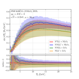
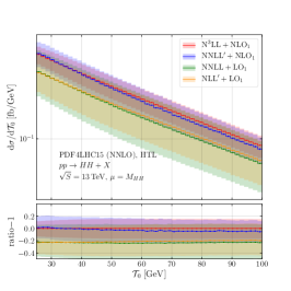
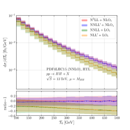
Figure 3: Resummed predictions matched to the appropriate fixed-order results at different accuracies for the $\mathcal{T}_{0}$ distribution in the peak (left), transition (centre) and tail (right) region.

We now discuss the numerical impact of the $\mathcal{T}_{0}$ resummation as well as that of the choice of the resummation cut $\mathcal{T}_{0,\rm re}^{\mathrm{cut}}$. In Fig. 3 we show resummed predictions for the $\mathcal{T}_{0}$ distribution divided into three different regions: peak, transition and tail. We present the resummed results at different resummation orders matched to the appropriate FO calculations: NLL^′+LO₁, NNLL+LO₁, NNLL^′+NLO₁ and N³LL + NLO₁. In this, and in all the following plots, we report both the statistical errors due to the Monte Carlo integration, which appear as vertical bars, as well as the scale variation band, obtained by the procedure previously discussed. The lower insets of the plots show instead the normalised relative ratios between the curves. As expected, the peak region at small $\mathcal{T}_{0}$ is where the resummation has the largest impact, which is reflected by a large spread among the predictions at different resummation accuracies. In the transition and tail regions the difference between the various predictions is driven by the FO accuracy, with LO₁ results being consistently smaller than the NLO₁ ones across the whole range. We observe a reasonable convergence of the perturbative predictions: the scale variations at $\rm N^{3}LL+NLO_{1}$ and $\rm NNLL^{\prime}+NLO_{1}$ are smaller than those at lower orders, especially in the peak and transition regions. We notice however that, contrary to what one might have anticipated, resummation effects are still visible up to values of $\mathcal{T}_{0}\lesssim 300$ GeV in the small difference between the N³LL and the NNLL^′ results, at the order of a few percent. This can be explained by the fact that the actual resummed variable is $\tau_{0}=\mathcal{T}_{0}/M_{HH}$, which, in this particular process, can be small even for relatively large values of $\mathcal{T}_{0}$, when $M_{HH}$ becomes very large.

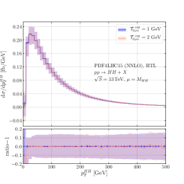
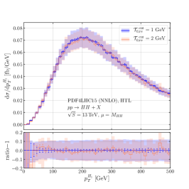
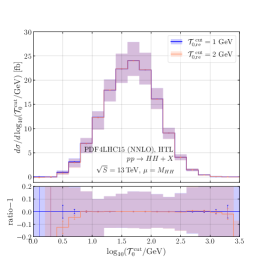
Figure 4: Comparison between $\mathcal{T}_{0,\rm re}^{\mathrm{cut}}=1,\>2\;\,\mathrm{GeV}$ at fixed $\mathcal{T}_{0,\rm ns}^{\mathrm{cut}}=0.5\;\,\mathrm{GeV}$ for $p_{T}^{HH}$ (left), $p_{T}^{H_{1}}$(centre) and $\mathcal{T}_{0}$ (right) distributions.

As discussed in the previous section, we use different cuts for the 0-jet resolution for the resummed and the nonsingular components. We remark that a variation in the value of $\mathcal{T}_{0,\rm re}^{\mathrm{cut}}$ only amounts to shifting part of the resummed contribution from the 0-jet bin to the spectrum, and vice versa. In general, the resummed calculation might be problematic when the soft and beam scales reach small values of the order $\Lambda_{\mathrm{QCD}}$, due to the running of the strong coupling. The introduction of profile scales that smoothly turn off the divergence, freezing the soft scale and preventing it from approaching $\Lambda_{\mathrm{QCD}}$, partially solves this problem, but renders the perturbative resummed calculation unreliable in that extreme region. Moreover, $\mathcal{T}_{0,\rm re}^{\mathrm{cut}}$ is eventually tied to the starting scale of the parton shower inside the 0-jet bin. Therefore, for both of the previous reasons, it is advisable not to push the $\mathcal{T}_{0,\rm re}^{\mathrm{cut}}$ to too small values. In Fig. 4 we study the dependence of the Geneva partonic results on the choice of $\mathcal{T}_{0,\rm re}^{\mathrm{cut}}$ for a fixed $\mathcal{T}_{0,\rm ns}^{\mathrm{cut}}=0.5$ GeV. As expected, this choice does not impact in a statistically significant way the distributions shown, which are the transverse momentum of the Higgs pair $p_{T}^{HH}$, the transverse momentum of the hardest Higgs boson $p_{T}^{H_{1}}$ and the zero-jettiness, respectively.

2.3 Nonsingular and power-suppressed corrections

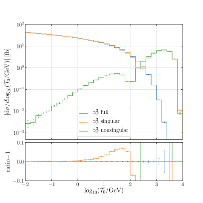
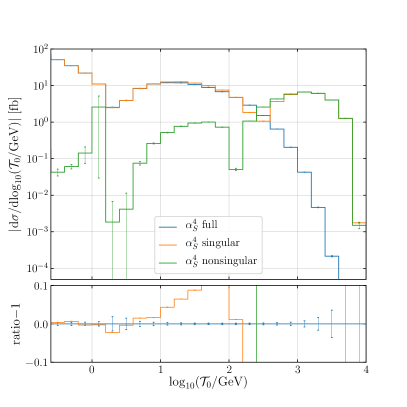
Figure 5: Singular and nonsingular contributions to the double Higgs production cross section as a function of $\mathcal{T}_{0}$ at NLO (left) and NNLO (right).

In the Geneva framework, all the contributions below the cut on the 0-jet resolution variable are given in Eq. (2.1). This expression is NNLO accurate and fully differential in the phase space $\Phi_{0}$. In principle one could use a local NNLO subtraction for the implementation of such terms. Alternatively, one can approximate, up to power corrections, the expression in Eq. (2.1) with

$$\frac{\widetilde{\mathrm{d}\sigma^{\rm MC}_{0}}}{\mathrm{d}\Phi_{0}}(\mathcal{T}_{0,\rm re}^{\mathrm{cut}},\mathcal{T}_{0,\rm ns}^{\mathrm{cut}})= \,\frac{\mathrm{d}\sigma^{\rm NNLL^{\prime}}}{\mathrm{d}\Phi_{0}}(\mathcal{T}_{0,\rm re}^{\mathrm{cut}})-\frac{\mathrm{d}\sigma^{\rm NNLL^{\prime}}}{\mathrm{d}\Phi_{0}}(\mathcal{T}_{0,\rm ns}^{\mathrm{cut}})\bigg{|}_{\rm NLO_{0}}+(B_{0}+V_{0})(\Phi_{0})$$

$$+\int B_{1}(\Phi_{1})\,\theta(\mathcal{T}_{0}(\Phi_{1})<\mathcal{T}_{0,\rm ns}^{\mathrm{cut}})\,\frac{\mathrm{d}\Phi_{1}}{\mathrm{d}\Phi_{0}}\,.$$ (27)

This formula only requires a NLO subtraction and the expansion of the resummed contribution at $\mathcal{O}(\alpha_{S})$ relative to the leading order. It is based on the fact that the singular and FO contributions cancel up to power corrections below the resolution cutoff at $\mathcal{O}(\alpha_{S}^{2})$. The cancellation between these two terms as a function of the resolution cutoff $\mathcal{T}_{0}$ is shown in Fig. 5 by plotting the absolute values of their central predictions, both at $\rm LO_{1}$, which is of absolute order $\alpha_{S}^{3}$, on the left and the pure $\alpha_{S}^{4}$ contribution on the right. We notice that the nonsingular distribution correctly approaches zero while the separate FO and singular contributions are diverging, both at order $\alpha_{S}^{3}$ and $\alpha_{S}^{4}$. This is despite the appearance of numerical instabilities in the region where the $\alpha_{S}^{4}$ nonsingular changes sign, around $\mathcal{T}_{0}\sim 1.5$ GeV. In practice, however, for any finite choice of $\mathcal{T}_{0,\rm ns}^{\mathrm{cut}}$ there are always remaining nonsingular power corrections below the cutoff, identified by the difference between Eq. (2.1) and (2.3), which reads

$$\frac{\mathrm{d}\Sigma^{(2)}_{\rm ns}}{\mathrm{d}\Phi_{0}}(\mathcal{T}_{0,\rm ns}^{\mathrm{cut}})= -\frac{\mathrm{d}\sigma^{\rm NNLL^{\prime}}}{\mathrm{d}\Phi_{0}}(\mathcal{T}_{0,\rm ns}^{\mathrm{cut}})\bigg{|}_{\rm NNLO_{0}}+\frac{\mathrm{d}\sigma^{\rm NNLL^{\prime}}}{\mathrm{d}\Phi_{0}}(\mathcal{T}_{0,\rm ns}^{\mathrm{cut}})\bigg{|}_{\rm NLO_{0}}+W_{0}(\Phi_{0})$$

$$+\int V_{1}(\Phi_{1})\,\theta(\mathcal{T}_{0}(\Phi_{1})<\mathcal{T}_{0,\rm ns}^{\mathrm{cut}})\,\frac{\mathrm{d}\Phi_{1}}{\mathrm{d}\Phi_{0}}$$

$$+\int B_{2}(\Phi_{2})\,\theta(\mathcal{T}_{0}(\Phi_{2})<\mathcal{T}_{0,\rm ns}^{\mathrm{cut}})\,\frac{\mathrm{d}\Phi_{2}}{\mathrm{d}\Phi_{0}}.$$ (28)

This term scales like a power correction in $\mathcal{T}_{0,\rm ns}^{\mathrm{cut}}/Q$ and is of $\mathcal{O}(\alpha_{S}^{2})$ relative to the Born contribution. We show its absolute size as a function of $\mathcal{T}_{0,\rm ns}^{\mathrm{cut}}$ in Fig. 6, as well as its relative size as a fraction of the NNLO cross section computed by Matrix Grazzini:2017mhc ; deFlorian:2016uhr on the right axis. For the results presented in this work we choose $\mathcal{T}_{0,\rm ns}^{\mathrm{cut}}=0.5\,\,\mathrm{GeV}$. The size of the missing corrections associated to that value is around $1.2\%$ of the total cross section. These missing contributions only affect events below the cutoff, and we can recover the exact NNLO cross section by reweighting these events by this difference. Note that, while we could have chosen smaller values of $\mathcal{T}_{0,\rm ns}^{\mathrm{cut}}$ to further minimise the impact of power corrections, lowering this value has shown to cause instabilities in the matrix elements used for our calculation.

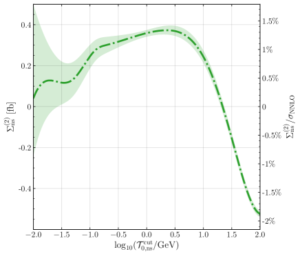
Figure 6: The neglected $\mathcal{O}(\alpha_{S}^{2})$ nonsingular contribution to the $\mathcal{T}_{0}$ cumulant $\Sigma_{\mathrm{NS}}^{(2)}$ as a function of $\mathcal{T}_{0,\rm ns}^{\mathrm{cut}}$. The green band represents the statistical uncertainty.

3 Details of the calculation and validation of NNLO results

We consider the process $pp\to HH+X$ and work in the HTL, taking into account only the gluon fusion production channel and requiring two on-shell Higgs bosons in the final state. The centre-of-mass energy considered is $\sqrt{S}=13$ TeV, and we use the following input parameters:

$$m_{H}=125.09\;\,\mathrm{GeV},\qquad v=246.32\;\,\mathrm{GeV},\qquad m_{t}=173.1\;\,\mathrm{GeV}.$$ (29)

We set both the factorisation and renormalisation scales to the invariant mass $M_{HH}$ of the Higgs pair, and we use the PDF4LHC15_nnlo_100 PDF Butterworth:2015oua set from LHAPDF 6 Buckley:2014ana , including the corresponding value of $\alpha_{S}(M_{Z})$. By default, we use the three-loop running of $\alpha_{S}$ for both Matrix and Geneva predictions. To evaluate the beam functions we use the beamfunc module of scetlib Billis:2019vxg ; scetlib . We set our resolution cutoffs as $\mathcal{T}_{0,\rm re}^{\mathrm{cut}}=1\;\,\mathrm{GeV}$, $\mathcal{T}_{0,\rm ns}^{\mathrm{cut}}=0.5\;\,\mathrm{GeV}$ and $\mathcal{T}_{1}^{\rm cut}=1\;\,\mathrm{GeV}$, which provide a reasonable compromise in terms of the size of the neglected power-suppressed terms and the stability of the singular-nonsingular cancellation.

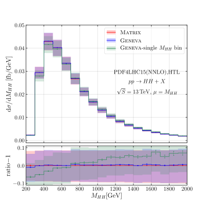
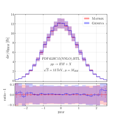
Figure 7: Comparison of the distribution for the Higgs pair invariant mass (left) and rapidity (right) between Matrix and Geneva.

All tree-level matrix elements are calculated using Recola Denner:2017wsf ; Denner:2017vms via a novel custom-built interface to Geneva, while all the one-loop terms are calculated through the standard Openloops Buccioni:2017yxi interface already used for processes previously implemented.

To validate the NNLO accuracy of the results obtained with Geneva, we compare our results to an independent calculation implemented in Matrix Grazzini:2017mhc ; deFlorian:2016uhr . Note that this comparison is done at partonic level, before interfacing to the parton shower. In Sec. 4 we will show the results at the showered level, highlighting how all the inclusive quantities presented in this section are well preserved by the shower stage. We report the result of this comparison in Fig. 7 and Fig. 8 where we show the invariant mass $M_{HH}$, the rapidity $y_{HH}$ of the Higgs pair, the transverse momentum of the softest of the two Higgs bosons and an observable depending on the rapidity difference between the two Higgs bosons, respectively. In Fig. 7, we show the comparison between Matrix (red), Geneva (blue) and, in the left panel, the Geneva line obtained by using Eq. (26) and Eq. (2.2.1) at face value (green). As anticipated, higher-order effects do play a significant role for the invariant-mass distribution of the Higgs pair. Indeed, we remind the reader that the green and blue lines here differ only by higher orders. To be precise, the blue line, which corresponds to the default Geneva prediction in this work, is obtained by computing the value $p$ of Eq. (26) – and thus Eq. (25) – in different bins of $M_{HH}$. The reason for this is given by the fact that, as explained in Sec. 2.2, the resummation we perform is for small $\tau_{0}$ values, which means that one can have large resummation effects even at large values of $\mathcal{T}_{0}$ and $M_{HH}$ provided their ratio is small. We have therefore combined various runs in different $M_{HH}$ bins, distributed more densely in the peak region where the cross section is larger. As can be seen, the difference between these two curves spans a range from $-5\%$ to roughly $+10\%$. While in general we find a reasonable agreement for these inclusive distributions within the uncertainty bands of the two calculations, obtained with the 3-point $\mu_{R}$ and $\mu_{F}$ variations, only the blue line shows perfect agreement with the Matrix result.

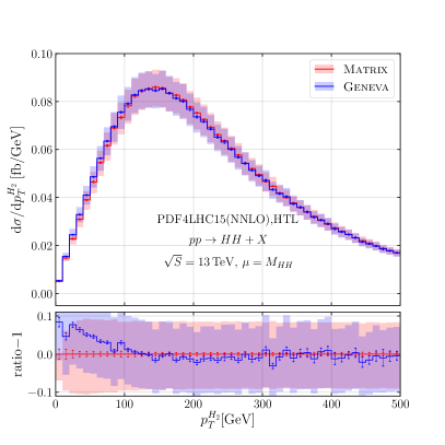
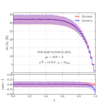
Figure 8: Comparison of the distributions for the transverse momentum of the softest Higgs boson (left) and the absolute value of their scattering angle (right) between Matrix and Geneva.

In Fig. 8 we report the comparison for the transverse momentum of the softest Higgs boson and the hyperbolic tangent of the rapidity difference between the two Higgs bosons, defined as

$$\chi=\tanh\left(\frac{|y_{H_{1}}-y_{H_{2}}|}{2}\right),$$ (30)

where $y_{H_{1},H_{2}}$ are the rapidities of each Higgs boson. Similarly to what is observed in the previous figure, we notice a good agreement, except in the regions of small $p_{T}^{H_{2}}$ or large $\chi$. These differences are expected, as although predictions obtained in the Geneva framework are NNLO accurate, they include a certain amount of higher-order effects, as well as power-suppressed corrections, which can lead to these kind of discrepancies. Note that these power corrections arise from a different physical treatment of kinematics compared to a FO calculation Ebert:2020dfc .

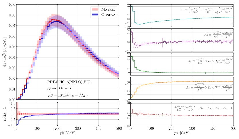
Figure 9: Comparison of the transverse momentum of the hardest Higgs boson between Matrix and Geneva (left) and breakdown of all relevant contributions that account for the differences. (right).

To see how such differences can arise between results that are formally at the same accuracy, we studied the discrepancies for $p_{T}$ of $H_{1}$ and $H_{2}$ and the $\chi$ distribution, and in the following we report detailed results for the transverse momentum distribution of the hardest Higgs boson, where these effects are largest. In Fig. 9, we report a breakdown of all possible sources of differences between a purely FO calculation such as that obtained via Matrix and the Geneva partonic prediction. All quantities shown in the sub-panels are expressed in terms of their relative size to the total distribution obtained with Matrix, and we detail each of them in the following. Firstly, it can be seen that in the small transverse momentum region we have a discrepancy – considerably bigger in size than that observed with the $p_{T}$ of the softest Higgs boson – which can reach $100\%$. In the upper right panel of Fig. 9 the first term that we look at is $A_{1}$, defined as

$$A_{1}\equiv\frac{\frac{\mathrm{d}\sigma^{\rm NNLL^{\prime}}}{\mathrm{d}p_{T}^{H_{1}}}-\frac{\mathrm{d}\sigma^{\rm NNLL^{\prime}}}{\mathrm{d}p_{T}^{H_{1}}}\bigg{|}_{\alpha_{S}^{2}}}{\frac{\mathrm{d}\sigma^{\textsc{Matrix}}}{\mathrm{d}p_{T}^{H_{1}}}},$$ (31)

which represents the difference between the resummed contribution and the resummed expanded up to $\mathcal{O}(\alpha_{S}^{2})$ coming from Geneva, normalised to the Matrix NNLO result. This difference is purely due to logarithmic terms beyond NNLO, and, as can be seen, in the region of interest gives rise to a large positive effect. In the second and third ratio plot we consider the contributions from projectable configurations with $\mathcal{T}_{0}<\mathcal{T}_{0,\rm ns}^{\mathrm{cut}}$ at relative $\mathcal{O}(\alpha_{S})$, $A_{2}$, and with $\mathcal{T}_{0}>\mathcal{T}_{0,\rm ns}^{\mathrm{cut}}$ and $\mathcal{T}_{1}<\mathcal{T}_{1}^{\mathrm{cut}}$ at relative $\mathcal{O}(\alpha_{S}^{2})$, $A_{3}$, defined as

$$A_{2}\equiv\frac{\frac{\mathrm{d}\sigma^{\rm NLO_{0}}_{\it diff}}{\mathrm{d}p_{T}^{H_{1}}}}{\frac{\mathrm{d}\sigma^{\textsc{Matrix}}}{\mathrm{d}p_{T}^{H_{1}}}},\qquad A_{3}\equiv\frac{\frac{\mathrm{d}\sigma^{\rm NLO_{1}}_{\it diff}}{\mathrm{d}p_{T}^{H_{1}}}\theta(\mathcal{T}_{0}>\mathcal{T}_{0,\rm ns}^{\mathrm{cut}})}{\frac{\mathrm{d}\sigma^{\textsc{Matrix}}}{\mathrm{d}p_{T}^{H_{1}}}}\,,$$ (32)

where the subscript diff refers to taking the difference between the observables evaluated on exact kinematical configurations, and those evaluated on projected kinematics below the respective resolution cutoffs. The effect of these two terms are pure power corrections as they arise from the projections used in Geneva to assign the event kinematics below the resolution cutoffs. Once again they are large and positive. Lastly, we examine the following quantity,

$$A_{4}\equiv\frac{\frac{\mathrm{d}\sigma^{\rm nonSing}_{\alpha_{S}^{2}}}{\mathrm{d}p_{T}^{H_{1}}}\theta(\mathcal{T}_{0}<\mathcal{T}_{0,\rm ns}^{\mathrm{cut}})}{\frac{\mathrm{d}\sigma^{\textsc{Matrix}}}{\mathrm{d}p_{T}^{H_{1}}}},$$ (33)

which represents the difference between the pure $\mathcal{O}(\alpha_{S}^{2})$ contributions of Geneva and Matrix below $\mathcal{T}_{0,\rm ns}^{\mathrm{cut}}$, normalised to the same value as before. This last term corresponds to the contribution in Eq. (2.3), projected onto $p_{T}^{H_{1}}$. Note that, in order to compute this quantity, one needs to take the $\mathcal{O}(\alpha_{S}^{2})$ from Matrix and subtract it from the resummed-expanded Geneva result at the same order. As shown in the respective sub-panel, this difference is negative and much larger than those considered above, thus being the main driver of the discrepancy. To conclude, and to show that there are no other possible sources of differences between Geneva and Matrix, we report in the last panel the difference between the partonic Geneva result and Matrix, subtracted of all the $A_{i}$ contributions which, as expected, is compatible with zero.

4 Parton Shower Interface

The general idea behind how the interface to the parton shower is performed in Geneva has been presented in various references, see in particular Ref. Alioli:2015toa for a detailed discussion. As such, in this context, we limit to a brief recap of the main features, highlighting the main novelties introduced for this specific process. The main issues one faces when matching a resummed calculation to the parton shower is to ensure that both the accuracy of the variable in which the resummation is performed and the accuracy of the parton shower are preserved.

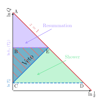
Figure 10: Lund Plane representation of shower emissions and their interplay with the resummation region.

In the specific case at hand, the resummation is performed in $\mathcal{T}_{N}$, from a hard scale $Q$ down to a lower scale $\mathcal{T}_{N}^{c}$. This can be represented graphically, as done in Fig. 10 with the purple-shaded triangular region (ACE), in the phase-space that an extra emission can have (commonly referred to as Lund Plane). As explained in the previous sections, Geneva produces events with $0,1$ or $2$ final-state partonic jets, each of which determines different lower scales for the resummation, corresponding to $\mathcal{T}_{0,\rm re}^{\mathrm{cut}}$, $\mathcal{T}_{1}^{\mathrm{cut}}$ and $\mathcal{T}_{1}\left(\Phi_{2}\right)$, respectively. The value of this scale corresponds to a diagonal line on the Lund Plane, and its intersection with the maximum available energy fraction an emission can have (E) sets the maximum relative transverse momentum of an emission ($k_{\perp}(\mathcal{T}_{N}^{c})$) given the lower resummation scale ($\mathcal{T}_{N}^{c}$). This, in turn, determines the starting scale for the parton shower. Now, the parton showers considered in this work produce emissions ordered in the relative transverse momentum, meaning that the allowed region for any emission from the parton shower is given by the trapezium (BCDE) spanning from the horizontal line determined by $k_{\perp}(\mathcal{T}_{N}^{c})$ to that determined by $\mathcal{T}_{N}^{c}$. This clearly produces a double-counted region, identified by the hashed triangle (BCE), where the shower could in principle produce emissions in the resummation region. To avoid this, we perform a veto procedure – much like what is done in matrix element merging techniques, such as CKKW-L Lonnblad:2001iq – that consists in discarding and retrying any event for which, after showering, we obtain a value of $\mathcal{T}_{N}>\mathcal{T}_{N}^{c}$.

To see that this procedure correctly ensures that no single shower emission can end up in the vetoed region, thus spoiling the NNLL accuracy of our $\mathcal{T}_{0}$ spectrum, recall that for any given final-state multiplicity $M$, $\mathcal{T}_{M}(\Phi_{M})=0$. Thus, for any one emission from the parton shower that produces a final state with $M+1$ partons, we have that $\mathcal{T}_{M}(\Phi_{M+1})=\mathcal{T}$ encodes the hardness of that emission, and can be compared to $\mathcal{T}_{N}^{c}$. In addition, $N$-jettiness is an additive variable of strictly positive terms, and the following relation, for a given final-state multiplicity, holds:

$$\mathcal{T}_{N}(\Phi_{M})\geq\mathcal{T}_{N+1}(\Phi_{M})\,.$$ (34)

To prove then that no single emission enters the vetoed region, consider the case the parton shower starts with a $N$-parton configuration, with $N=0,1,2$. After the parton shower, we end up with a $N+k$ partonic final state, where $k$ stands for the total emissions performed by the shower. Our veto implies that

$$\mathcal{T}_{N}(\Phi_{N+k})\leq\mathcal{T}_{N}^{c}\,.$$ (35)

Combining the previous relations, we get that

$$\mathcal{T}_{N+k-1}(\Phi_{N+k})\leq\mathcal{T}_{N+k-2}(\Phi_{N+k})\leq\dots\leq\mathcal{T}_{N}(\Phi_{N+k})\leq\mathcal{T}_{N}^{c}\,,$$ (36)

which implies that also the hardness of each of the $k$th emissions has to be smaller than $\mathcal{T}_{N}^{c}$, given the additive property of $N$-jettiness. This means that the final events accepted after the veto could always be generated via a sequence of $\mathcal{T}$-ordered emissions, even if the actual showering might not have respected that condition locally. To better clarify the meaning of Eq. (36), let us consider the following explicit example. Imagine that we start the parton shower from a configuration with two partons, $\Phi_{2}$, which represents the bulk of the events generated by Geneva after the resummation of $\mathcal{T}_{0}$ and $\mathcal{T}_{1}$ has been performed at the parton level. Thus, the value of $\mathcal{T}_{N}^{c}=\mathcal{T}_{1}(\Phi_{2})$ determines the starting scale of the parton shower $k_{\perp}(\mathcal{T}_{1}(\Phi_{2}))$. An additional emission of the shower has a hardness of $\mathcal{T}=\mathcal{T}_{2}(\Phi_{3})$ which by construction has to be smaller than $\mathcal{T}_{N}^{c}$ to respect the veto condition. When a second emission is performed its hardness is given by $\mathcal{T}=\mathcal{T}_{3}(\Phi_{4})\leq\mathcal{T}_{2}(\Phi_{4})$ which by construction needs to be smaller than $\mathcal{T}_{1}(\Phi_{2})$ to satisfy the veto. Iterating this, one can reconstruct the full chain of inequalities appearing in Eq. (36). As the variable $N$-jettiness is additive, it is also true that the hardness of the first emission is constrained by the veto to be lower than the lower resummation scale. Clearly this does not impose any ordering between the hardness of the two emissions, $\mathcal{T}_{2}(\Phi_{3})$ and $\mathcal{T}_{3}(\Phi_{4})$, it just implies that they are both lower than $\mathcal{T}_{1}(\Phi_{2})$. Note that, as a consequence, this implies that the accuracy of the parton shower is not spoiled by our matching procedure. In fact, the resummation region has a higher accuracy than that of the shower, and in the shower region there is no double-counted contribution. Thus the accuracy on any observable computed with this matching is at least as accurate as the parton shower is.

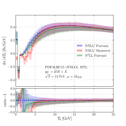
Figure 11: Comparison of the effects of the shower and the effects of the N³LL resummation.

The argument presented above does not imply that the resummed variable – $\mathcal{T}_{0}$ in this case – is numerically preserved, as shown in Fig. 11. However, it can be seen that the shift in the spectrum induced by the parton shower is of similar size as that given by including higher-order effects in the resummation. Compared to other colour-singlet production processes studied in the past with the Geneva framework, one can notice that, in this case, the impact of the shower on the $\mathcal{T}_{0}$ distribution can be numerically sizeable. This has to do with two key differences with respect to other processes Alioli:2021egp ; Alioli:2019qzz ; Cridge:2021hfr ; Alioli:2021qbf . First, since this process is dominated by gluon channels, we expect effects due to gluon emissions to be scaled by a factor $C_{A}/C_{F}\sim 2$. Second, this is one of the first processes which features a hard scale, $M_{HH}$, which spans different orders of magnitude and does not really present a sharp peak. This implies that even at relatively large values of $\mathcal{T}_{0}$ – given that the scale we have control over is $\tau_{0}=\mathcal{T}_{0}/M_{HH}$ – one can have a small value of $\tau_{0}$ with $M_{HH}$ still large. The consequence is that, for any fixed value of $\mathcal{T}_{0}$, the large logarithmic terms associated to this Higgs pair production can be significantly larger than the corresponding terms for the same value of $\mathcal{T}_{0}$ in other processes.

In addition, as a validation of the matching with the shower, we show in the left panel of Fig. 12 how the shower correctly preserves the spectrum of fully inclusive variables such as the invariant mass of the Higgs pair. This implies that the total inclusive cross section is also preserved by the shower.

To further study the impact of parton showers, we extend Geneva’s default shower interface to Pythia 8 to both Dire Hoche:2015sya , as implemented in Pythia 8, and the default shower in Sherpa Gleisberg:2008ta ; Sherpa:2019gpd ; Schumann:2007mg . These three parton showers differ most notably by the choice of the evolution variable, which, together with the starting scale imposed by our matching, determines how much of the phase space away from the strict soft and collinear limits is available to the parton shower.

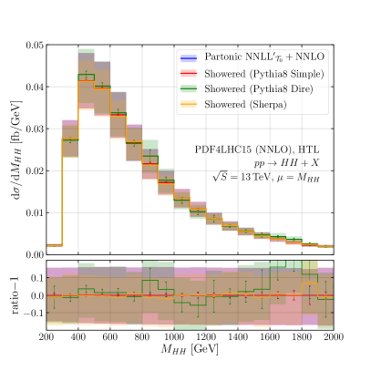
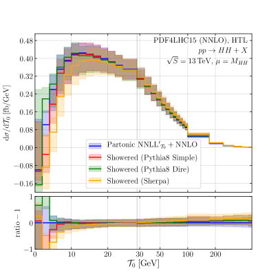
Figure 12: Comparison between the partonic and showered for the di-Higgs invariant-mass (left panel) and the $\mathcal{T}_{0}$ (right panel) distributions in Geneva, Geneva + Pythia 8, Geneva + Dire and Geneva + Sherpa.

As shown in Fig. 12, right panel, the impact of the choice of the parton shower can be relatively large for small ($\leq 10$ GeV) values of $\mathcal{T}_{0}$. Indeed, while all the three showers present deviations from the partonic result of roughly the same magnitude, they differ significantly among each other, which can be approximately viewed as a shower matching uncertainty. The fact that this process can be highly sensitive to different choices of evolution variables, and thus different parton showers, was shown in Ref. Jones:2017giv . The net result is that, for the default choice of the evolution variable, the Catani-Seymour based shower as implemented in Sherpa has an evolution variable $t$ on average larger than that of Dire, leading to its phase space reach being more constrained. This is reflected in the suppression in the small $\mathcal{T}_{0}$ region.

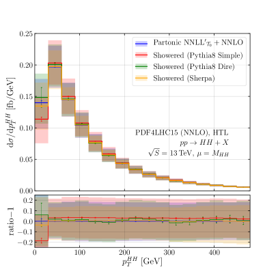
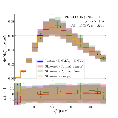
Figure 13: Comparison between the partonic and showered for $p_{T}^{HH}$ (left) and $p_{T}^{H_{1}}$ (right) in Geneva, Geneva + Pythia 8, Geneva + Dire and Geneva + Sherpa.

Lastly, in Fig. 13 we show how the different showers affect the transverse momentum of the Higgs pair system and that of the hardest Higgs boson. In this case, although in principle the parton shower is not required to preserve either of these observables, we see that all shower predictions largely agree among themselves and with the partonic result, aside from the very first bin where they agree within uncertainties. This is likely due to the fact that partonic events produced by Geneva already feature both a $\mathcal{T}_{0}$ and a $\mathcal{T}_{1}$ resummation, both of which have a non-trivial interplay with the transverse momentum distribution of the colour-singlet system.

5 Conclusions

With the detailed study of the properties of the Higgs boson, discovered ten years ago at the LHC, set to dominate the research focus of the next twenty to fifty years, the ability to constrain the self-coupling of the Higgs boson is one of the fundamental milestones. While many of such properties are largely dominated by the reach of the experimental set-up, the Higgs self-coupling determination is instead limited by statistics, from the experimental point of view, and by uncertainties in the theoretical predictions for both signal and background. Indeed, even after the high-luminosity phase of the LHC, it is predicted that with the current theoretical knowledge the value of the self-coupling will only be constrained to about $50\%$ DiMicco:2019ngk .

From the theoretical standpoint, the process affecting the most the determination of this fundamental parameter of the Standard Model Lagrangian, at hadron colliders, is the production of a Higgs pair in the gluon-gluon fusion channel. Similarly to the production of a single Higgs boson this process proceeds via a top-quark loop, thus rendering the inclusion of higher corrections in the exact theory, with full heavy-quark mass dependence, highly non-trivial. Indeed only NLO corrections are known exactly Borowka:2016ehy for this process, as they require a state-of-the-art two-loop calculation with both internal and external masses. Nevertheless, similarly to the single Higgs case, one can expand the Lagrangian of the Standard Model in inverse powers of the top-quark mass thus constructing an effective theory where the top quark is decoupled and Higgs bosons couple directly to gluons, usually referred to as HTL. While this approach is known to be a poor approximation for double Higgs production, it still provides useful insights if the main interest is to study the effects of the inclusion of higher-order QCD corrections, resummation and the interface to the parton shower.

In this work we take the latter approach and present an implementation of the production of a pair of Higgs bosons via gluon-gluon fusion in the HTL in Geneva. By employing this framework we are able to produce fully-differential NNLO results matched to a $\mathcal{T}_{0}$ NNLL^′ resummation, using the SCET formalism, further interfaced to the parton shower. We show that, using a traditional value of the hard scale in the argument of the logarithms, such as the Higgs pair invariant mass, resummation effects affect exclusive observables at much larger values than in processes previously studied. This is a consequence of the fact that the $M_{HH}$ distribution spans over a large range. Moreover, we study in detail how the inclusion of resummation and subleading power corrections can impact the comparison with standard fixed-order results, such as those obtained with Matrix, tracking down all sources of possible differences at higher order. Lastly, we present and discuss the impact of interfacing our partonic predictions to different parton showers and find that this process is subject to large parton shower effects. This is the first step towards a more comprehensive estimation of parton shower matching uncertainties.

It is clear that, while the approach taken in this work to use the HTL works well as far as we only discuss the effect of pure QCD higher-order effects, in order to develop a realistic event generator for the production of a Higgs pair, we need to include mass effects if not in an exact way, at least in some approximation. Indeed, the natural continuation of this work is to explore ways, such as those devised in Ref. Davies:2019nhm , to include partial top-quark mass effects in our implementation.

Appendix A Hard function for $gg\to HH$ in the $\overline{\rm MS}$ scheme

In this appendix, we report the necessary ingredients to obtain the hard function in the $\overline{\mathrm{MS}}$ scheme. Its perturbative expansion, in a generic subtraction scheme $X$ reads

$$H_{X}=\left(\frac{\alpha_{S}}{4\pi}\right)^{2}\left[H^{(0)}+\frac{\alpha_{S}}{4\pi}H^{(1)}_{X}+\left(\frac{\alpha_{S}}{4\pi}\right)^{2}H^{(2)}_{X}+\mathcal{O}(\alpha_{S}^{3})\right].$$ (37)

Note that $H^{(0)}$ is scheme independent, since it is given by the cross section at LO, defined, for this process, as

$$H^{(0)} =\frac{s\,C^{2}_{\rm LO}}{144\,v^{4}}.$$ (38)

Defining $s$ as the squared centre-of-mass energy of the process, $v$ the vacuum expectation value, $m_{H}$ the Higgs boson mass one has

$$C_{\rm LO}=\frac{6\lambda v^{2}}{s-m^{2}_{H}}-1,\qquad 2\lambda v^{2}=m_{H}^{2}\quad\mathrm{and}\quad v^{4}=\frac{1}{2G_{F}^{2}}\,.$$ (39)

In the Catani subtraction scheme ($X=C$), the expressions for the one- and two-loop coefficients of the hard function are given in Refs. deFlorian:2013uza and Grigo:2014jma . To extract the results needed for the implementation in Geneva, we start by defining

$$H_{C}^{(i)}=\frac{\mathrm{d}\sigma_{\mathrm{fin}}^{(i)}}{\mathrm{d}t}\frac{\mathrm{d}t}{\mathrm{d}\Phi_{2}}$$ (40)

where we used the following Jacobian,

$$\frac{\mathrm{d}\Phi_{2}}{\mathrm{d}t}=\frac{1}{8\pi s}\frac{1}{\Gamma\!\left(1-\epsilon\right)}\left[\frac{s\left(s-4m_{H}^{2}\right)-\left(t-u\right)^{2}}{16\pi s}\right]^{-\epsilon}\,.$$ (41)

We can express the coefficients of Eq. (37) in the $\overline{\rm MS}$ scheme ($X=\overline{\rm MS}$) by exploiting the following relations

$$H^{(1)}_{\overline{\rm MS}} =H^{(1)}_{C}+\lim_{\epsilon\to 0}2\,{\rm Re}\,[2\,\mathcal{I}^{(1)}(\epsilon)+\mathcal{Z}^{(1)}(\epsilon)]\,H^{(0)},$$

$$H^{(2)}_{\overline{\rm MS}} =H^{(2)}_{C}+\lim_{\epsilon\to 0}\bigg{\{}2\,{\rm{Re}}\,[2\,\mathcal{I}^{(1)}(\epsilon)+\mathcal{Z}^{(1)}(\epsilon)]\bigg{\}}\,H^{(1)}_{C}+\bigg{\{}|\lim_{\epsilon\to 0}[2\,\mathcal{I}^{(1)}(\epsilon)+\mathcal{Z}^{(1)}(\epsilon)]|^{2}$$

$$+2{\rm{Re}}\lim_{\epsilon\to 0}\bigg{(}4\,\mathcal{I}^{(2)}(\epsilon)+2\,\mathcal{I}^{(1)}(\epsilon)[2\,\mathcal{I}^{(1)}(\epsilon)+\mathcal{Z}^{(1)}(\epsilon)]+\mathcal{Z}^{(2)}(\epsilon)\bigg{)}\bigg{\}}H^{(0)}\,,$$ (42)

where for simplicity we dropped the $\mu$ dependence from the $H^{(i)}_{X}$, $\mathcal{I}^{(i)}$ and $\mathcal{Z}^{(i)}$. In the equation above, $\mathcal{I}^{(i)}$ are the perturbative coefficients of the $\mathcal{I}$ operator defined as deFlorian:2012za

$$\mathcal{I}(\epsilon,\mu)=1+\left(\frac{\alpha_{S}}{2\pi}\right)\mathcal{I}^{(1)}(\epsilon,\mu)+\left(\frac{\alpha_{S}}{2\pi}\right)^{2}\mathcal{I}^{(2)}(\epsilon,\mu)+\mathcal{O}(\alpha_{S}^{3})\,,$$ (43)

where

$$\mathcal{I}^{(1)}(\epsilon,\mu) =-\bigg{(}\frac{\mu^{2}}{-s}\bigg{)}^{\epsilon}\frac{\exp(\epsilon\,\gamma_{E})}{\Gamma(1-\epsilon)}\bigg{(}C_{g}\frac{1}{\epsilon^{2}}+\gamma_{g}\frac{1}{\epsilon}\bigg{)},$$

$$\mathcal{I}^{(2)}(\epsilon,\mu) =\bigg{(}\frac{\mu^{2}}{-s}\bigg{)}^{\epsilon}\frac{\exp(\epsilon\gamma_{E})}{72\,\Gamma(1-\epsilon)\epsilon^{4}}\bigg{\{}12\epsilon(C_{g}+\epsilon\gamma_{g})(11C_{A}-2n_{f})$$

$$-\frac{36\exp(\epsilon\gamma_{E})}{(\Gamma(1-\epsilon)}\bigg{(}\frac{\mu^{2}}{-s}\bigg{)}^{\epsilon}(C_{g}+\epsilon\gamma_{g})^{2}\ +\epsilon\bigg{(}\frac{\mu^{2}}{-s}\bigg{)}^{\epsilon}\bigg{[}36\epsilon^{2}H_{g}$$

$$+2(3+5\epsilon)(C_{g}+2\epsilon\gamma_{g})n_{f}+C_{A}(C_{g}+2\epsilon\gamma_{g})(-33-67\epsilon+3\epsilon\pi^{2})\bigg{]}\bigg{\}}\,,$$ (44)

and for gluon-initiated processes one finds

$$C_{g} =C_{A},\qquad\gamma_{g}=\frac{\beta_{0}}{2},$$

$$H_{g} =C^{2}_{A}\bigg{(}\frac{1}{2}\zeta_{3}+\frac{5}{12}+\frac{11\pi^{2}}{144}\bigg{)}-C_{A}n_{f}\bigg{(}\frac{29}{27}+\frac{\pi^{2}}{72}\bigg{)}+\frac{1}{2}C_{F}n_{f}+\frac{5}{27}n^{2}_{f}\,.$$ (45)

The $\mathcal{Z}^{(i)}$ in Eq. (37) are obtained from the following expansion of the $\mathcal{Z}$ factor Becher:2009qa ,

$$\mathcal{Z}^{-1}(\epsilon,\mu)=1+\left(\frac{\alpha_{S}}{4\pi}\right)\mathcal{Z}^{(1)}(\epsilon,\mu)+\left(\frac{\alpha_{S}}{4\pi}\right)^{2}\mathcal{Z}^{(2)}(\epsilon,\mu)+\mathcal{O}(\alpha_{S}^{3})\,,$$ (46)

where

$$\mathcal{Z}^{(1)}(\epsilon,\mu) =-\frac{\Gamma^{\prime}_{0}}{4\epsilon^{2}}-\frac{\mathbf{\Gamma}_{0}}{2\epsilon},$$

$$\mathcal{Z}^{(2)}(\epsilon,\mu) =\frac{(\Gamma^{\prime}_{0})^{2}}{32\epsilon^{4}}+\frac{3\beta_{0}\Gamma^{\prime}_{0}+2\Gamma^{\prime}_{0}\mathbf{\Gamma}_{0}}{16\epsilon^{3}}+\frac{4\beta_{0}\mathbf{\Gamma}_{0}+2\mathbf{\Gamma}_{0}^{2}-\Gamma^{\prime}_{1}}{16\epsilon^{2}}-\frac{\mathbf{\Gamma}_{1}}{4\epsilon}\,,$$ (47)

and

$$\mathbf{\Gamma}_{i} =-C_{A}\Gamma_{i}\ln\bigg{(}\frac{\mu^{2}}{-s}\bigg{)}+2\gamma^{g}_{i},\qquad\Gamma^{\prime}_{i}=-2C_{A}\Gamma_{i}\,,$$

$$\gamma^{g}_{1} =C^{2}_{A}\bigg{(}-\frac{692}{27}+\frac{11\pi^{2}}{18}+2\zeta_{3}\bigg{)}+C_{A}T_{F}n_{f}\bigg{(}\frac{256}{27}-\frac{2\pi^{2}}{9}\bigg{)}+4C_{F}T_{F}n_{f}\,,$$ (48)

with $C_{A}$, $C_{F}$ the colour factors, $n_{f}$ the number of light flavours and $T_{F}=1/2$. Considering Eq. (A) and setting $\mu^{2}=s$, we find the following results for the translation to the $\overline{\rm MS}$ scheme of the hard function coefficients

$$H^{(1)}_{\overline{\rm MS}} =H^{(1)}_{C}+\frac{7C_{A}\pi^{2}}{3}H^{(0)},$$

$$H^{(2)}_{\overline{\rm MS}} =H^{(2)}_{C}+\frac{7C_{A}\pi^{2}}{3}H^{(1)}_{C}$$

$$+\bigg{(}\frac{167}{6}C^{2}_{A}\pi^{2}-\frac{367}{54}C_{A}n_{f}\pi^{2}+\frac{11n^{2}_{f}\pi^{2}}{27}+\frac{73}{36}C^{2}_{A}\pi^{4}-\frac{11}{3}C^{2}_{A}\zeta_{3}+\frac{2}{3}C_{A}n_{f}\zeta_{3}\bigg{)}H^{(0)}.$$ (49)

Finally, in order to restore the exact $\mu$ dependence of the hard function we use the RGE equation

$$\frac{\mathrm{d}}{\mathrm{d}\ln(\mu^{2})}H(\mu^{2})={\rm{Re}}[\mathbf{\Gamma}(\mu^{2})]\,H(\mu^{2}).$$ (50)

Taking the first order of the expansion $\mathcal{O}(\alpha_{S}^{3})$, we have:

$$\frac{\mathrm{d}}{\mathrm{d}\ln(\mu^{2})}H^{(1)}(\mu^{2})-2\beta_{0}H^{(0)} ={\rm Re}[\mathbf{\Gamma}_{0}(\mu^{2})]H^{(0)}\,,$$ (51)

having used

$$\frac{1}{4\pi}\frac{\mathrm{d}}{\mathrm{d}\ln(\mu^{2})}\alpha_{S}=-\bigg{(}\frac{\alpha_{S}}{4\pi}\bigg{)}^{2}\sum_{n=0}\bigg{(}\frac{\alpha_{S}}{4\pi}\bigg{)}^{n}\beta_{n}.$$ (52)

For the second order of the expansion $\mathcal{O}(\alpha_{S}^{4})$ in Eq. (50) we have

$$\frac{\mathrm{d}}{\mathrm{d}\ln(\mu^{2})}H^{(2)}(\mu^{2})-2\beta_{1}H^{(0)}-3\beta_{0}H^{(1)}(\mu^{2})={\rm Re}[\mathbf{\Gamma}_{0}(\mu^{2})]H^{(1)}(\mu^{2})+{\rm Re}[\mathbf{\Gamma}_{1}(\mu^{2})]H^{(0)}\,,$$ (53)

where $\beta_{1}$ is defined in Eq. (2.1). In conclusion, the hard function in the $\overline{\rm MS}$ scheme is given by

$$H_{\overline{\rm MS}}(\mu^{2})=\left(\frac{\alpha_{S}}{4\pi}\right)^{2}\left[H^{(0)}(\mu^{2})+\left(\frac{\alpha_{S}}{4\pi}\right)H^{(1)}_{\overline{\rm MS}}(\mu^{2})+\left(\frac{\alpha_{S}}{4\pi}\right)^{2}H^{(2)}_{\overline{\rm MS}}(\mu^{2})+\mathcal{O}(\alpha_{S}^{3})\right]\,,$$ (54)

where

$$H^{(0)}(\mu^{2}) =H^{(0)},$$

$$H^{(1)}_{\overline{\rm MS}}(\mu^{2}) =H^{(1)}_{\overline{\rm MS}}(s)-2C_{A}\ln^{2}\left(\frac{\mu^{2}}{s}\right)H^{(0)},$$

$$H^{(2)}_{\overline{\rm MS}}(\mu^{2}) =H^{(2)}_{\overline{\rm MS}}(s)-H^{(1)}_{\overline{\rm MS}}(s)\left[2C_{A}\ln^{2}\left(\frac{\mu^{2}}{s}\right)-\frac{11}{3}C_{A}\ln\left(\frac{\mu^{2}}{s}\right)+\frac{2}{3}n_{f}\ln\left(\frac{\mu^{2}}{s}\right)\right]$$

$$+H^{(0)}\bigg{[}\ln\left(\frac{\mu^{2}}{s}\right)\left(-\frac{772}{27}C^{2}_{A}+\frac{76}{27}C_{A}n_{f}+\frac{11}{9}C^{2}_{A}\pi^{2}-\frac{2}{9}C_{A}n_{f}\pi^{2}+4C^{2}_{A}\zeta_{3}\right)$$

$$+\ln^{2}\left(\frac{\mu^{2}}{s}\right)\left(-\frac{134}{9}C^{2}_{A}+\frac{20}{9}C_{A}n_{f}+\frac{2}{3}C^{2}_{A}\pi^{2}\right)+\ln^{3}\left(\frac{\mu^{2}}{s}\right)\left(-\frac{22}{9}C^{2}_{A}+\frac{4}{9}C_{A}n_{f}\right)$$

$$+2C^{2}_{A}\ln^{4}\left(\frac{\mu^{2}}{s}\right)\bigg{]}.$$ (55)

References

- (1) ATLAS collaboration, Observation of a new particle in the search for the Standard Model Higgs boson with the ATLAS detector at the LHC, Phys. Lett. B 716 (2012) 1 [1207.7214].
- (2) CMS collaboration, Observation of a New Boson at a Mass of 125 GeV with the CMS Experiment at the LHC, Phys. Lett. B 716 (2012) 30 [1207.7235].
- (3) ATLAS collaboration, Measurement of the properties of Higgs boson production at TeV in the channel using fb-1 of collision data with the ATLAS experiment, 2207.00348.
- (4) CMS collaboration, Measurements of the Higgs boson production cross section and couplings in the W boson pair decay channel in proton-proton collisions at = 13 TeV, 2206.09466.
- (5) CMS collaboration, Search for boosted Higgs boson decay to a charm quark-antiquark pair in proton-proton collisions at = 13 TeV, 2211.14181.
- (6) ATLAS collaboration, Direct constraint on the Higgs-charm coupling from a search for Higgs boson decays into charm quarks with the ATLAS detector, Eur. Phys. J. C 82 (2022) 717 [2201.11428].
- (7) CMS collaboration, Search for nonresonant Higgs boson pair production in final state with two bottom quarks and two tau leptons in proton-proton collisions at = 13 TeV, 2206.09401.
- (8) CMS collaboration, Search for Higgs boson pairs decaying to WWWW, WW, and in proton-proton collisions at = 13 TeV, 2206.10268.
- (9) ATLAS collaboration, Search for resonant and non-resonant Higgs boson pair production in the decay channel using 13 TeV collision data from the ATLAS detector, 2209.10910.
- (10) ATLAS collaboration, Search for resonant pair production of Higgs bosons in the final state using collisions at = 13 TeV with the ATLAS detector, Phys. Rev. D 105 (2022) 092002 [2202.07288].
- (11) J. Alison et al., Higgs boson potential at colliders: Status and perspectives, Rev. Phys. 5 (2020) 100045 [1910.00012].
- (12) G. Degrassi, P. P. Giardino, F. Maltoni and D. Pagani, Probing the Higgs self coupling via single Higgs production at the LHC, JHEP 12 (2016) 080 [1607.04251].
- (13) G. Degrassi, M. Fedele and P. P. Giardino, Constraints on the trilinear Higgs self coupling from precision observables, JHEP 04 (2017) 155 [1702.01737].
- (14) F. Maltoni, D. Pagani, A. Shivaji and X. Zhao, Trilinear Higgs coupling determination via single-Higgs differential measurements at the LHC, Eur. Phys. J. C 77 (2017) 887 [1709.08649].
- (15) E. W. N. Glover and J. J. van der Bij, HIGGS BOSON PAIR PRODUCTION VIA GLUON FUSION, Nucl. Phys. B 309 (1988) 282.
- (16) O. J. P. Eboli, G. C. Marques, S. F. Novaes and A. A. Natale, TWIN HIGGS BOSON PRODUCTION, Phys. Lett. B 197 (1987) 269.
- (17) T. Plehn, M. Spira and P. M. Zerwas, Pair production of neutral Higgs particles in gluon-gluon collisions, Nucl. Phys. B 479 (1996) 46 [hep-ph/9603205].
- (18) S. Dawson, S. Dittmaier and M. Spira, Neutral Higgs boson pair production at hadron colliders: QCD corrections, Phys. Rev. D 58 (1998) 115012 [hep-ph/9805244].
- (19) D. de Florian and J. Mazzitelli, Higgs Boson Pair Production at Next-to-Next-to-Leading Order in QCD, Phys. Rev. Lett. 111 (2013) 201801 [1309.6594].
- (20) D. de Florian, M. Grazzini, C. Hanga, S. Kallweit, J. M. Lindert, P. Maierhöfer et al., Differential Higgs Boson Pair Production at Next-to-Next-to-Leading Order in QCD, JHEP 09 (2016) 151 [1606.09519].
- (21) L.-B. Chen, H. T. Li, H.-S. Shao and J. Wang, Higgs boson pair production via gluon fusion at N3LO in QCD, Phys. Lett. B 803 (2020) 135292 [1909.06808].
- (22) P. Banerjee, S. Borowka, P. K. Dhani, T. Gehrmann and V. Ravindran, Two-loop massless QCD corrections to the four-point amplitude, JHEP 11 (2018) 130 [1809.05388].
- (23) S. Borowka, N. Greiner, G. Heinrich, S. P. Jones, M. Kerner, J. Schlenk et al., Higgs Boson Pair Production in Gluon Fusion at Next-to-Leading Order with Full Top-Quark Mass Dependence, Phys. Rev. Lett. 117 (2016) 012001 [1604.06447].
- (24) S. Borowka, N. Greiner, G. Heinrich, S. P. Jones, M. Kerner, J. Schlenk et al., Full top quark mass dependence in Higgs boson pair production at NLO, JHEP 10 (2016) 107 [1608.04798].
- (25) J. Baglio, F. Campanario, S. Glaus, M. Mühlleitner, M. Spira and J. Streicher, Gluon fusion into Higgs pairs at NLO QCD and the top mass scheme, Eur. Phys. J. C 79 (2019) 459 [1811.05692].
- (26) J. Baglio, F. Campanario, S. Glaus, M. Mühlleitner, J. Ronca, M. Spira et al., Higgs-Pair Production via Gluon Fusion at Hadron Colliders: NLO QCD Corrections, JHEP 04 (2020) 181 [2003.03227].
- (27) M. Grazzini, G. Heinrich, S. Jones, S. Kallweit, M. Kerner, J. M. Lindert et al., Higgs boson pair production at NNLO with top quark mass effects, JHEP 05 (2018) 059 [1803.02463].
- (28) D. De Florian and J. Mazzitelli, Soft gluon resummation for Higgs boson pair production including finite Mt effects, JHEP 08 (2018) 156 [1807.03704].
- (29) L.-B. Chen, H. T. Li, H.-S. Shao and J. Wang, The gluon-fusion production of Higgs boson pair: N3LO QCD corrections and top-quark mass effects, JHEP 03 (2020) 072 [1912.13001].
- (30) G. Ferrera and J. Pires, Transverse-momentum resummation for Higgs boson pair production at the LHC with top-quark mass effects, JHEP 02 (2017) 139 [1609.01691].
- (31) G. Heinrich, S. P. Jones, M. Kerner, G. Luisoni and E. Vryonidou, NLO predictions for Higgs boson pair production with full top quark mass dependence matched to parton showers, JHEP 08 (2017) 088 [1703.09252].
- (32) S. Jones and S. Kuttimalai, Parton Shower and NLO-Matching uncertainties in Higgs Boson Pair Production, JHEP 02 (2018) 176 [1711.03319].
- (33) G. Heinrich, S. P. Jones, M. Kerner, G. Luisoni and L. Scyboz, Probing the trilinear Higgs boson coupling in di-Higgs production at NLO QCD including parton shower effects, JHEP 06 (2019) 066 [1903.08137].
- (34) R. Frederix, S. Frixione, V. Hirschi, F. Maltoni, O. Mattelaer, P. Torrielli et al., Higgs pair production at the LHC with NLO and parton-shower effects, Phys. Lett. B 732 (2014) 142 [1401.7340].
- (35) F. Maltoni, E. Vryonidou and M. Zaro, Top-quark mass effects in double and triple Higgs production in gluon-gluon fusion at NLO, JHEP 11 (2014) 079 [1408.6542].
- (36) P. Maierhöfer and A. Papaefstathiou, Higgs Boson pair production merged to one jet, JHEP 03 (2014) 126 [1401.0007].
- (37) J. Grigo, J. Hoff, K. Melnikov and M. Steinhauser, On the Higgs boson pair production at the LHC, Nucl. Phys. B 875 (2013) 1 [1305.7340].
- (38) J. Grigo, K. Melnikov and M. Steinhauser, Virtual corrections to Higgs boson pair production in the large top quark mass limit, Nucl. Phys. B 888 (2014) 17 [1408.2422].
- (39) J. Grigo, J. Hoff and M. Steinhauser, Higgs boson pair production: top quark mass effects at NLO and NNLO, Nucl. Phys. B 900 (2015) 412 [1508.00909].
- (40) G. Degrassi, P. P. Giardino and R. Gröber, On the two-loop virtual QCD corrections to Higgs boson pair production in the Standard Model, Eur. Phys. J. C 76 (2016) 411 [1603.00385].
- (41) R. Gröber, A. Maier and T. Rauh, Reconstruction of top-quark mass effects in Higgs pair production and other gluon-fusion processes, JHEP 03 (2018) 020 [1709.07799].
- (42) R. Bonciani, G. Degrassi, P. P. Giardino and R. Gröber, Analytical Method for Next-to-Leading-Order QCD Corrections to Double-Higgs Production, Phys. Rev. Lett. 121 (2018) 162003 [1806.11564].
- (43) J. Davies, G. Mishima, M. Steinhauser and D. Wellmann, Double Higgs boson production at NLO in the high-energy limit: complete analytic results, JHEP 01 (2019) 176 [1811.05489].
- (44) G. Mishima, High-Energy Expansion of Two-Loop Massive Four-Point Diagrams, JHEP 02 (2019) 080 [1812.04373].
- (45) J. Davies, G. Heinrich, S. P. Jones, M. Kerner, G. Mishima, M. Steinhauser et al., Double Higgs boson production at NLO: combining the exact numerical result and high-energy expansion, JHEP 11 (2019) 024 [1907.06408].
- (46) J. Davies and M. Steinhauser, Three-loop form factors for Higgs boson pair production in the large top mass limit, JHEP 10 (2019) 166 [1909.01361].
- (47) J. Davies, F. Herren, G. Mishima and M. Steinhauser, Real corrections to Higgs boson pair production at NNLO in the large top quark mass limit, JHEP 01 (2022) 049 [2110.03697].
- (48) L. Bellafronte, G. Degrassi, P. P. Giardino, R. Gröber and M. Vitti, Gluon fusion production at NLO: merging the transverse momentum and the high-energy expansions, JHEP 07 (2022) 069 [2202.12157].
- (49) S. Alioli, C. W. Bauer, C. Berggren, F. J. Tackmann and J. R. Walsh, Drell-Yan production at NNLL’+NNLO matched to parton showers, Phys. Rev. D92 (2015) 094020 [1508.01475].
- (50) S. Alioli, A. Broggio, S. Kallweit, M. A. Lim and L. Rottoli, Higgsstrahlung at NNLL′+NNLO matched to parton showers in GENEVA, Phys. Rev. D 100 (2019) 096016 [1909.02026].
- (51) S. Alioli, A. Broggio, A. Gavardi, S. Kallweit, M. A. Lim, R. Nagar et al., Resummed predictions for hadronic Higgs boson decays, JHEP 04 (2021) 254 [2009.13533].
- (52) S. Alioli, A. Broggio, A. Gavardi, S. Kallweit, M. A. Lim, R. Nagar et al., Precise predictions for photon pair production matched to parton showers in GENEVA, JHEP 04 (2021) 041 [2010.10498].
- (53) S. Alioli, A. Broggio, A. Gavardi, S. Kallweit, M. A. Lim, R. Nagar et al., Next-to-next-to-leading order event generation for boson pair production matched to parton shower, Phys. Lett. B 818 (2021) 136380 [2103.01214].
- (54) S. Alioli, A. Broggio, A. Gavardi, S. Kallweit, M. A. Lim, R. Nagar et al., Matching NNLO to parton shower using N3LL colour-singlet transverse momentum resummation in GENEVA, 2102.08390.
- (55) Höche, Stefan and Li, Ye and Prestel, Stefan, Higgs-boson production through gluon fusion at NNLO QCD with parton showers, Phys. Rev. D 90 (2014) 054011 [1407.3773].
- (56) P. F. Monni, P. Nason, E. Re, M. Wiesemann and G. Zanderighi, MiNNLOPS: a new method to match NNLO QCD to parton showers, JHEP 05 (2020) 143 [1908.06987].
- (57) J. M. Campbell, S. Höche, H. T. Li, C. T. Preuss and P. Skands, Towards NNLO+PS Matching with Sector Showers, 2108.07133.
- (58) M. Grazzini, S. Kallweit and M. Wiesemann, Fully differential NNLO computations with MATRIX, Eur. Phys. J. C 78 (2018) 537 [1711.06631].
- (59) S. Dawson, C. Kao, Y. Wang and P. Williams, QCD Corrections to Higgs Pair Production in Bottom Quark Fusion, Phys. Rev. D 75 (2007) 013007 [hep-ph/0610284].
- (60) J. Davies, R. Gröber, A. Maier, T. Rauh and M. Steinhauser, Top quark mass dependence of the Higgs boson-gluon form factor at three loops, Phys. Rev. D 100 (2019) 034017 [1906.00982].
- (61) S. Alioli, C. W. Bauer, C. Berggren, F. J. Tackmann, J. R. Walsh et al., Matching Fully Differential NNLO Calculations and Parton Showers, JHEP 1406 (2014) 089 [1311.0286].
- (62) I. W. Stewart, F. J. Tackmann and W. J. Waalewijn, N-Jettiness: An Inclusive Event Shape to Veto Jets, Phys. Rev. Lett. 105 (2010) 092002 [1004.2489].
- (63) A. Gavardi, Next-to-next-to-leading order predictions for diboson production in hadronic scattering combined with parton showers, Ph.D. thesis, Milan Bicocca U., 2023.
- (64) S. Alioli, G. Billis, A. Broggio, A. Gavardi, S. Kallweit, M. A. Lim et al., Refining the GENEVA method for Higgs boson production via gluon fusion, 2301.11875.
- (65) S. Alioli, C. W. Bauer, S. Guns and F. J. Tackmann, Underlying event sensitive observables in Drell-Yan production using GENEVA, Eur. Phys. J. C 76 (2016) 614 [1605.07192].
- (66) C. F. Berger, C. Marcantonini, I. W. Stewart, F. J. Tackmann and W. J. Waalewijn, Higgs Production with a Central Jet Veto at NNLL+NNLO, JHEP 1104 (2011) 092 [1012.4480].
- (67) I. W. Stewart, F. J. Tackmann and W. J. Waalewijn, Factorization at the LHC: From PDFs to Initial State Jets, Phys. Rev. D 81 (2010) 094035 [0910.0467].
- (68) S. Moch, J. A. M. Vermaseren and A. Vogt, The Three loop splitting functions in QCD: The Nonsinglet case, Nucl. Phys. B 688 (2004) 101 [hep-ph/0403192].
- (69) A. Vogt, S. Moch and J. A. M. Vermaseren, The Three-loop splitting functions in QCD: The Singlet case, Nucl. Phys. B 691 (2004) 129 [hep-ph/0404111].
- (70) G. P. Korchemsky and A. V. Radyushkin, Renormalization of the Wilson Loops Beyond the Leading Order, Nucl. Phys. B 283 (1987) 342.
- (71) O. V. Tarasov, A. A. Vladimirov and A. Y. Zharkov, The Gell-Mann-Low Function of QCD in the Three Loop Approximation, Phys. Lett. B 93 (1980) 429.
- (72) S. A. Larin and J. A. M. Vermaseren, The Three loop QCD Beta function and anomalous dimensions, Phys. Lett. B 303 (1993) 334 [hep-ph/9302208].
- (73) R. Kelley, M. D. Schwartz, R. M. Schabinger and H. X. Zhu, The two-loop hemisphere soft function, Phys. Rev. D84 (2011) 045022 [1105.3676].
- (74) P. F. Monni, T. Gehrmann and G. Luisoni, Two-Loop Soft Corrections and Resummation of the Thrust Distribution in the Dijet Region, JHEP 08 (2011) 010 [1105.4560].
- (75) D. de Florian and J. Mazzitelli, Two-loop virtual corrections to Higgs pair production, Phys. Lett. B 724 (2013) 306 [1305.5206].
- (76) J. Gaunt, M. Stahlhofen and F. J. Tackmann, The Gluon Beam Function at Two Loops, JHEP 08 (2014) 020 [1405.1044].
- (77) M. A. Ebert, B. Mistlberger and G. Vita, -jettiness beam functions at N3LO, JHEP 09 (2020) 143 [2006.03056].
- (78) T. van Ritbergen, J. A. M. Vermaseren and S. A. Larin, The Four loop beta function in quantum chromodynamics, Phys. Lett. B 400 (1997) 379 [hep-ph/9701390].
- (79) A. von Manteuffel, E. Panzer and R. M. Schabinger, Cusp and collinear anomalous dimensions in four-loop QCD from form factors, Phys. Rev. Lett. 124 (2020) 162001 [2002.04617].
- (80) D. Bertolini, M. P. Solon and J. R. Walsh, Integrated and Differential Accuracy in Resummed Cross Sections, Phys. Rev. D 95 (2017) 054024 [1701.07919].
- (81) J. Butterworth et al., PDF4LHC recommendations for LHC Run II, J. Phys. G43 (2016) 023001 [1510.03865].
- (82) A. Buckley, J. Ferrando, S. Lloyd, K. Nordström, B. Page, M. Rüfenacht et al., LHAPDF6: parton density access in the LHC precision era, Eur. Phys. J. C75 (2015) 132 [1412.7420].
- (83) G. Billis, M. A. Ebert, J. K. L. Michel and F. J. Tackmann, A toolbox for and 0-jettiness subtractions at , Eur. Phys. J. Plus 136 (2021) 214 [1909.00811].
- (84) M. A. Ebert, J. K. L. Michel, F. J. Tackmann et al., SCETlib: A C++ Package for Numerical Calculations in QCD and Soft-Collinear Effective Theory, DESY-17-099 http://scetlib.desy.de.
- (85) A. Denner, J.-N. Lang and S. Uccirati, Recola2: REcursive Computation of One-Loop Amplitudes 2, Comput. Phys. Commun. 224 (2018) 346 [1711.07388].
- (86) A. Denner, J.-N. Lang and S. Uccirati, NLO electroweak corrections in extended Higgs Sectors with RECOLA2, JHEP 07 (2017) 087 [1705.06053].
- (87) F. Buccioni, S. Pozzorini and M. Zoller, On-the-fly reduction of open loops, Eur. Phys. J. C 78 (2018) 70 [1710.11452].
- (88) M. A. Ebert, J. K. L. Michel, I. W. Stewart and F. J. Tackmann, Drell-Yan resummation of fiducial power corrections at N3LL, JHEP 04 (2021) 102 [2006.11382].
- (89) L. Lonnblad, Correcting the colour-dipole cascade model with fixed order matrix elements, JHEP 05 (2002) 046 [hep-ph/0112284].
- (90) T. Cridge, M. A. Lim and R. Nagar, production at NNLO+PS accuracy in GENEVA, 2105.13214.
- (91) S. Höche and S. Prestel, The midpoint between dipole and parton showers, Eur. Phys. J. C 75 (2015) 461 [1506.05057].
- (92) T. Gleisberg, S. Hoeche, F. Krauss, M. Schonherr, S. Schumann, F. Siegert et al., Event generation with SHERPA 1.1, JHEP 02 (2009) 007 [0811.4622].
- (93) Sherpa collaboration, Event Generation with Sherpa 2.2, SciPost Phys. 7 (2019) 034 [1905.09127].
- (94) S. Schumann and F. Krauss, A Parton shower algorithm based on Catani-Seymour dipole factorisation, JHEP 03 (2008) 038 [0709.1027].
- (95) D. de Florian and J. Mazzitelli, A next-to-next-to-leading order calculation of soft-virtual cross sections, JHEP 12 (2012) 088 [1209.0673].
- (96) T. Becher and M. Neubert, On the Structure of Infrared Singularities of Gauge-Theory Amplitudes, JHEP 06 (2009) 081 [0903.1126].