Quasar UV/X-ray relation luminosity distances are shorter than reverberation-measured radius-luminosity relation luminosity distances

Abstract

We use measurements of 59/58 quasars (QSOs), over a redshift range $0.0041\leq z\leq 1.686$, to do a comparative study of the radius–luminosity ($R-L$) and X-ray$-$UV luminosity ($L_{X}-L_{UV}$) relations and the implication of these relations for cosmological parameter estimation. By simultaneously determining $R-L$ or $L_{X}-L_{UV}$ relation parameters and cosmological parameters in six different cosmological models, we find that both $R-L$ and $L_{X}-L_{UV}$ relations are standardizable but provide only weak cosmological parameter constraints, with $L_{X}-L_{UV}$ relation data favoring larger current non-relativistic matter density parameter $\Omega_{m0}$ values than $R-L$ relation data and most other available data. We derive $L_{X}-L_{UV}$ and $R-L$ luminosity distances for each of the sources in the six cosmological models and find that $L_{X}-L_{UV}$ relation luminosity distances are shorter than $R-L$ relation luminosity distances as well as standard flat $\Lambda$CDM model luminosity distances. This explains why $L_{X}-L_{UV}$ relation QSO data favor larger $\Omega_{m0}$ values than do $R-L$ relation QSO data or most other cosmological measurements. While our sample size is small and only spans a small $z$ range, these results indicate that more work is needed to determine whether the $L_{X}-L_{UV}$ relation can be used as a cosmological probe.

1 Introduction

If general relativity provides an accurate description of gravity on cosmological scales, dark energy is responsible for the observed current accelerated cosmological expansion and contributes $\sim 70\%$ of the current cosmological energy budget. In the standard spatially-flat $\Lambda$CDM cosmological model (Peebles, 1984) dark energy is the cosmological constant $\Lambda$ and non-relativistic cold dark matter (CDM) contributes $\sim 25\%$ of the current cosmological energy budget with non-relativistic baryonic matter contributing $\sim 5\%$. While the standard model is reasonably consistent with low redshift $z\lesssim 2.3$ observations (Scolnic et al., 2018; Yu et al., 2018; eBOSS Collaboration, 2021) and $z\sim 1100$ measurements (Planck Collaboration, 2020), it might not be able to accommodate some data (Di Valentino et al., 2021a; Perivolaropoulos & Skara, 2022; Abdalla et al., 2022).

A new reliable cosmological probe, especially one in the largely unexplored part of redshift space between the highest $z\sim 2.3$ baryon acoustic oscillation (BAO) measurements and cosmic microwave background anisotropy data at $z\sim 1100$, might help clarify whether the standard flat $\Lambda$CDM model needs to be improved on.

The last decade has seen the initial development of a number of such probes, including H ii starburst galaxy apparent magnitude observations which reach to $z\sim 2.5$ (Mania & Ratra, 2012; Chávez et al., 2014; González-Morán et al., 2021; Cao et al., 2020, 2021a, 2022a; Johnson et al., 2022; Mehrabi et al., 2022), quasar (hereafter QSO) angular size observations which reach to $z\sim 2.7$ (Cao et al., 2017; Ryan et al., 2019; Cao et al., 2020, 2021b; Zheng et al., 2021; Lian et al., 2021), Mg ii and C iv reverberation mapped QSO observations which reach to $z\sim 3.4$ (Zajaček et al., 2021; Khadka et al., 2021a, 2022b; Cao et al., 2022e), and gamma-ray burst (GRB) observations which reach to $z\sim 8.2$ (Wang et al., 2016, 2022a; Fana Dirirsa et al., 2019; Demianski et al., 2021; Khadka & Ratra, 2020c; Khadka et al., 2021b; Hu et al., 2021; Luongo & Muccino, 2021; Cao et al., 2022b, c, d; Dainotti et al., 2022a; Liu et al., 2022; Jia et al., 2022; Liang et al., 2022; Kumar et al., 2022).

Another potentially promising probe makes use of QSO X-ray and UV flux measurements which reach to $z\sim 7.5$ (Risaliti & Lusso, 2015, 2019; Khadka & Ratra, 2020a, b, 2021, 2022; Lusso et al., 2020; Rezaei et al., 2022; Luongo et al., 2022; Hu & Wang, 2022; Colgáin et al., 2022; Dainotti et al., 2022b; Petrosian et al., 2022; Li et al., 2022; Wang et al., 2022b; Pourojaghi et al., 2022) and is the main subject of our paper. With the progress of knowledge of such QSO properties and an increase in the number of these sources, such QSO data have been used to constrain cosmological model parameters. Strong constraints, and tension with the standard flat $\Lambda$CDM model, have been claimed (Risaliti & Lusso, 2019; Lusso et al., 2020) from a method based on an assumed non-linear relation between the QSO UV and X-ray luminosities, $L_{UV}$ and $L_{X}$ (Tananbaum et al., 1979; Zamorani et al., 1981; Avni & Tananbaum, 1986; Steffen et al., 2006; Just et al., 2007; Green et al., 2009; Young et al., 2010; Lusso et al., 2010; Grupe et al., 2010; Vagnetti et al., 2010). We note that the analyses of Risaliti & Lusso (2019) and Lusso et al. (2020) were approximate and based on incorrect assumptions (Khadka & Ratra, 2020a, b, 2021, 2022; Banerjee et al., 2021; Petrosian et al., 2022). The correct technique for analyses of $L_{X}-L_{UV}$ relation QSO data was developed in Khadka & Ratra (2020a). Here one must use these QSO data to simultaneously determine the $L_{X}-L_{UV}$ relation parameters and the cosmological model parameters. In this case, one must also study a number of different cosmological models to determine whether $L_{X}-L_{UV}$ relation parameter values are independent of the assumed cosmological model, and if they are, then these QSOs are standardizable and the circularity problem is circumvented. Unfortunately, the most recent Lusso et al. (2020) QSO compilation is not standardizble (Khadka & Ratra, 2021, 2022), because the $L_{X}-L_{UV}$ relation parameters depend on the assumed cosmological model and on redshift (Khadka & Ratra, 2021, 2022). See Dainotti et al. (2022b), Li et al. (2022), and Wang et al. (2022b) for more recent discussions of the redshift evolution, but note that out of these studies, only Li et al. (2022) do analyses of redshift-space subsets of these QSO data (as did Khadka & Ratra, 2021, 2022). Khadka & Ratra (2022) found that the largest of the seven QSO sub-samples in the Lusso et al. (2020) compilation, the SDSS-4XMM, i.e. the one that contains about 2/3 of the total QSOs, has an $L_{X}-L_{UV}$ relation that depends on the cosmological model as well as on redshift and is the main, but possibly not only, cause of the problem with the Lusso et al. (2020) compilation.

Recently, there has been considerable progress in the development of another QSO probe that is based on the correlation between the rest-frame time-delay of the broad-line response with respect to the variable continuum and the monochromatic continuum luminosity, known as the radius-luminosity ($R-L$) relation. The application of this relation was proposed over a decade ago (Watson et al., 2011; Haas et al., 2011; Bentz et al., 2013; Czerny et al., 2013) but it was successfully implemented only recently by using Mg ii and C iv time delays (Zajaček et al., 2021; Khadka et al., 2021a, 2022b; Cao et al., 2022e); see also Karas et al. (2021) and Czerny et al. (2022) for recent reviews. We note that using currently available H$\beta$ measurements is still problematic (Khadka et al., 2022a). Although H$\beta$ $R-L$ relation parameters are independent of the assumed cosmological model, the constraints are weak, favour decelerated expansion, and are in 2$\sigma$ tension with better established probes. Corrections related to the Eddington ratio introduced in the fixed flat $\Lambda$CDM model (Martínez-Aldama et al., 2019; Martínez-Aldama et al., 2020; Panda, 2022; Panda & Marziani, 2022) do not yield a significant improvement when cosmological parameters are set free (Khadka et al., 2022a). Future reassessment of H$\beta$ time delays, including a careful removal of outliers (Czerny et al., 2021), appears necessary as an attempt to resolve this H$\beta$ QSO problem. In contrast to H$\beta$ results, cosmological constraints based on the Mg ii and C iv $R-L$ relations are consistent with the standard flat $\Lambda$CDM model.

Given the problems with the Lusso et al. (2020) $L_{X}-L_{UV}$ QSO compilation, X-ray detected Mg ii reverberation-measured QSOs provide a unique opportunity to determine whether the QSO $L_{X}-L_{UV}$ relation can be used as a cosmological probe. X-ray detected Mg ii QSOs can be used to derive $L_{X}-L_{UV}$ relation and cosmological model parameter values and these can be compared to the corresponding $R-L$ relation and cosmological model parameter values. Such a sample provides a unique opportunity to probe potential systematic effects of these two relations that are independent of each other. The only correlation present is between corresponding UV flux densities at 2500 Å (for the $L_{X}-L_{UV}$ relation) and 3000 Å (for the $R-L$ relation). However, the measurements of the Mg ii line-emission time-delay and the X-ray flux density at 2 keV are independent of each other.

Khadka et al. (2021a) and Khadka et al. (2022b) have shown that a larger compilation of Mg ii $R-L$ QSOs are standardizable and so can be used as a cosmological probe, and we find that the smaller sample of 58 X-ray detected Mg ii $R-L$ QSOs, over $0.0041\leq z\leq 1.686$, that we study here also share these attributes. We find that the corresponding $L_{X}-L_{UV}$ relation for these QSOs are also standardizable, which is encouraging but possibly a consequence of the much smaller sample size and smaller redshift range compared to those of the Lusso et al. (2020) $L_{X}-L_{UV}$ QSO compilation. However, we go on to derive $L_{X}-L_{UV}$ and $R-L$ luminosity distances for each of the 58 sources in six different cosmological models and find that $L_{X}-L_{UV}$ relation luminosity distances are shorter than $R-L$ relation luminosity distances as well as standard flat $\Lambda$CDM model luminosity distances. This result explains why $L_{X}-L_{UV}$ relation QSO data favor larger current non-relativistic matter density parameter $\Omega_{m0}$ values than do $R-L$ relation QSO data or most other cosmological measurements. While our sample size is small and these QSOs span only $0.0041\leq z\leq 1.686$, our results indicate that more work is needed before we can determine whether the $L_{X}-L_{UV}$ relation can be used as a cosmological probe.

Our paper is structured as follows. In Sec. 2 we introduce the cosmological models and $R-L$ and $L_{X}-L_{UV}$ relations and their parameters. The data we use are described in Sec. 3. The method we use to infer parameter values and uncertainties is outlined in Sec. 4. In Sec. 5 we present the main results obtained using the two independent methods. We conclude in Sec. 6.

2 Cosmological models and parameters

In this study we constrain cosmological model parameters, $R-L$ relation parameters, and $L_{X}-L_{UV}$ relation parameters in three pairs of dark-energy general-relativistic cosmological models with flat and non-flat spatial geometries, so in total six cosmological models, by using QSO measurements. This allows us to compare two sets of cosmological constraints, those derived using the $R-L$ relation and those derived using the $L_{X}-L_{UV}$ relation. On the other hand, since we constrain correlation parameters for both these correlation relations using the same set of sources, these results can indicate which correlation relation better holds for the QSOs we consider.

Observational data used in this paper are QSO time-delays and 3000 Å, 2500 Å, and 2 keV flux densities. The $R-L$ and $L_{X}-L_{UV}$ relations involve luminosity so flux needs to be converted to luminosity. To do this we need the luminosity distance $D_{L}(z,\mathbf{p})$ for each source. Given a cosmological model, the luminosity distance (in cm) can be computed as a function of redshift ($z$) and cosmological parameters ($\mathbf{p}$),

Here $c$ is the speed of light, $H_{0}$ is the Hubble constant, $\Omega_{k0}$ is the current value of the spatial curvature energy density parameter, and $D_{C}(z,\mathbf{p})$ is the comoving distance. This is computed as a function of $z$ and $\mathbf{p}$ for a given cosmological model from

$$D_{C}(z,\mathbf{p})=c\int^{z}_{0}\frac{dz^{\prime}}{H(z^{\prime},\mathbf{p})},$$ (2)

where $H(z,\mathbf{p})$ is the Hubble parameter, and is given below for the six cosmological models we use in this paper. The luminosity distance can be used to compute the luminosity $L(z,\mathbf{p})$, in units of ${\rm erg\,s^{-1}}$ (or the luminosity per frequency in units of ${\rm erg\,s^{-1}Hz^{-1}}$) from the flux density $F$, in units of ${\rm erg\,s^{-1}cm^{-2}}$ (or the flux density per frequency in units of ${\rm erg\,s^{-1}cm^{-2}Hz^{-1}}$), through

$$L(z,\mathbf{p})=4\pi D_{L}(z,\mathbf{p})^{2}F.$$ (3)

Observations indicate that for Mg ii QSOs the reverberation measured time delay $\tau$ and $L_{3000}(z,\mathbf{p})$, the monochromatic luminosity at 3000 Å, obey an $R-L$ relation (Czerny et al., 2019, 2022; Zajaček et al., 2020, 2021; Homayouni et al., 2020; Martínez-Aldama et al., 2020; Yu et al., 2021, 2022; Khadka et al., 2021a, 2022b; Cao et al., 2022e)

$$\log\left({\frac{\tau}{\rm day}}\right)=\beta+\gamma\log\left[{\frac{L_{3000}(z,\mathbf{p})}{10^{44}\,{\rm erg\,s^{-1}}}}\right]\,,$$ (4)

where $\log$ = $\log_{10}$ and the intercept $\beta$ and the slope $\gamma$ are free parameters to be determined from data concurrently with the cosmological-model parameters $\mathbf{p}$ that influence the $R-L$ relation through $L_{3000}(z,\mathbf{p})$, see Sec. 4. Using instead the measured flux density $F_{3000}$ and the luminosity distance, eq. (4) can be expressed as

$$\log{\left(\frac{\tau}{\rm day}\right)}= \beta+\gamma\log(4\pi)$$ (5)

$$+\gamma\left[\log\left(\frac{F_{3000}}{{\rm erg\,s^{-1}cm^{-2}}}\right)-44\right]+2\gamma\log(D_{L}),$$

Observations also indicate that QSO X-ray (2 keV) and UV (2500 Å) luminosities, $L_{X}$ and $L_{UV}$ (expressed per frequency), are correlated (Tananbaum et al., 1979; Zamorani et al., 1981; Avni & Tananbaum, 1986; Steffen et al., 2006; Just et al., 2007; Green et al., 2009; Young et al., 2010; Lusso et al., 2010; Grupe et al., 2010; Vagnetti et al., 2010) through the $L_{X}-L_{UV}$ relation. This relation is

$$\log\left(\frac{L_{X}}{{\rm erg\,s^{-1}Hz^{-1}}}\right)=\beta+\gamma\log\left(\frac{L_{UV}}{10^{29}\,{\rm erg\,s^{-1}Hz^{-1}}}\right),$$ (6)

where the slope $\gamma$ and the intercept $\beta$ are free parameters [the difference between these free parameters and those of eq. (4) should be clear from the context] to be determined from the data concurrently with the cosmological-model parameters, as described in Sec. 4. Luminosities and flux densities are related through the luminosity distance, so eq. (6) can be rewritten as

$$\log{\left(\frac{F_{X}}{\rm erg\,s^{-1}cm^{-2}Hz^{-1}}\right)} =\beta+(\gamma-1)\log(4\pi)+2(\gamma-1)\log(D_{L})$$

$$+\gamma\left[\log\left(\frac{F_{UV}}{{\rm erg\,s^{-1}cm^{-2}Hz^{-1}}}\right)-29\right],$$ (7)

where $F_{UV}$ and $F_{X}$ are the quasar UV and X-ray flux densities (per frequency), and $L_{UV}=4\pi D_{L}^{2}F_{UV}$ is scaled to $10^{29}\,{\rm erg\,s^{-1}cm^{-2}Hz^{-1}}$, which tightens the constraints for the intercept $\beta$.

For the computation of luminosity distance, the fundamental quantity needed is the Hubble parameter $H(z)$ which is computed using the assumed cosmological model. In what follows we give the functional form of $H(z)$ for each cosmological model we use.

In the $\Lambda$CDM model the Hubble parameter is

$$H(z,\mathbf{p})=H_{0}\sqrt{\Omega_{m0}(1+z)^{3}+\Omega_{k0}(1+z)^{2}+\Omega_{\Lambda}}\,.$$ (8)

Here $\Omega_{\Lambda}$ is the cosmological constant density parameter and the three energy density parameters obey the current energy budget equation $\Omega_{m0}$ + $\Omega_{k0}$ + $\Omega_{\Lambda}$ = 1. In the spatially non-flat $\Lambda$CDM model we choose $\Omega_{m0}$, $\Omega_{k0}$, and $H_{0}$ to be the free parameters. For the spatially-flat $\Lambda$CDM model we choose the same set of free parameters but now set $\Omega_{k0}=0$ as required for flat spatial hypersurfaces.

In the XCDM dynamical dark energy parametrization the Hubble parameter is

$$H(z,\mathbf{p})=H_{0}\sqrt{\Omega_{m0}(1+z)^{3}+\Omega_{k0}(1+z)^{2}+\Omega_{X0}(1+z)^{3(1+\omega_{X})}},$$ (9)

where $\Omega_{X0}$ is the current value of the $X$-fluid dark energy density parameter and, together with $\Omega_{m0}$ and $\Omega_{k0}$, it obeys the current energy budget equation $\Omega_{m0}$ + $\Omega_{k0}$ + $\Omega_{X0}$ = 1. The equation of state parameter of the $X$-fluid $\omega_{X}=P_{X}/\rho_{X}$, where $P_{X}$ and $\rho_{X}$ are the pressure and energy density of the $X$-fluid. In the spatially non-flat XCDM parametrization we choose $\Omega_{m0}$, $\Omega_{k0}$, $\omega_{X}$, and $H_{0}$ to be the free parameters. For the spatially-flat XCDM parametrization we choose the same set of free parameters but now set $\Omega_{k0}=0$ as required for flat spatial hypersurfaces. When $\omega_{X}=-1$ the XCDM parametrization reduces to the $\Lambda$CDM model.

In the $\phi$CDM model the dynamical dark energy is a scalar field $\phi$ (Peebles & Ratra, 1988; Ratra & Peebles, 1988; Pavlov et al., 2013). Here we assume that the scalar field potential energy density $V(\phi)$ is an inverse power law of $\phi$ and this potential energy density, defined next, determines the scalar field dark energy density parameter $\Omega_{\phi}(z,\alpha)$. The functional form of $V(\phi)$ we use is

$$V(\phi)=\frac{1}{2}\kappa m_{p}^{2}\phi^{-\alpha},$$ (10)

where $m_{p}$ and $\alpha$ are the Planck mass and a positive parameter respectively, and $\kappa$ is a constant whose value is determined by using the shooting method to guarantee that the current energy budget equation $\Omega_{m0}+\Omega_{k0}+\Omega_{\phi}(z=0,\alpha)=1$ holds.

With this potential energy density, coupled differential equations, i.e. the scalar field equation of motion and the Friedmann equation, govern the dynamics of $\phi$ and the cosmological scale factor $a$. For a spatially homogeneous scalar field these two coupled equations of motion are

$$\ddot{\phi}+3\frac{\dot{a}}{a}\dot{\phi}-\frac{1}{2}\alpha\kappa m_{p}^{2}\phi^{-\alpha-1}=0,$$ (11)

$$\left(\frac{\dot{a}}{a}\right)^{2}=\frac{8\pi}{3m_{p}^{2}}\left(\rho_{m}+\rho_{\phi}\right)-\frac{k}{a^{2}}.$$ (12)

Here an overdot indicates a derivative with respect to time, $k$ is positive, zero, and negative for closed, flat, and open spatial geometry (corresponding to $\Omega_{k0}<0,=0,{\rm and}>0$), $\rho_{m}$ is the non-relativistic matter energy density, and the scalar field energy density is given by

$$\rho_{\phi}=\frac{m^{2}_{p}}{32\pi}\left[\dot{\phi}^{2}+\kappa m^{2}_{p}\phi^{-\alpha}\right].$$ (13)

The numerical solution of the coupled differential equations (11) and (12) is used to compute $\rho_{\phi}$ and

$$\Omega_{\phi}(z,\alpha)=\frac{8\pi\rho_{\phi}}{3m^{2}_{p}H^{2}_{0}}.$$ (14)

The Hubble parameter in the $\phi$CDM model is

$$H(z,\mathbf{p})=H_{0}\sqrt{\Omega_{m0}(1+z)^{3}+\Omega_{k0}(1+z)^{2}+\Omega_{\phi}\left(z,\alpha\right)}.$$ (15)

In the spatially non-flat $\phi$CDM model we choose $\Omega_{m0}$, $\Omega_{k0}$, $\alpha$, and $H_{0}$ to be the free parameters. For the spatially-flat $\phi$CDM model we choose the same set of free parameters but now set $\Omega_{k0}=0$ as required for flat spatial hypersurfaces. When $\alpha=0$ the $\phi$CDM model reduces to the $\Lambda$CDM model.

QSO data cannot constrain $H_{0}$ because there is a degeneracy between the intercept ($\beta$) of the correlation relations and $H_{0}$, so we set $H_{0}$ to 70 km s^-1 Mpc^-1 in all QSO data-only analyses.

3 Data description

By cross-matching the previously studied 78 reverberation-mapped Mg ii QSOs (Khadka et al., 2021a) with the XMM-Newton X-ray source catalog (4XMMDR11), we found that 58 of the 78 sources were also detected in the X-ray domain. The X-ray fluxes in the 4XMMDR11 catalog are measured at various energy bands and listed in units of erg s^-1 cm^-2. For our study, we used spline interpolation to determine the X-ray fluxes at 2 keV energy, i.e. $F_{\rm 2keV}$. In our analysis, we use 2 keV flux densities per unit frequency $F_{X}\equiv F_{\rm 2keV}/\nu_{\rm 2keV}$ (in ${\rm erg\,s^{-1}\,cm^{-2}\,Hz^{-1}}$). For the Mg ii QSOs, we had flux densities at 3000 Å, $F_{3000}$ in ${\rm erg\,s^{-1}cm^{-2}}$, available from the continuum flux determination in the surroundings of the broad Mg ii line. To obtain UV flux densities at 2500 Å we used the continuum slope $\alpha_{\nu}=-0.45\pm 0.01$ of the mean quasar spectrum from Vanden Berk et al. (2001), specifically $F_{UV}=F_{3000,\nu}(2500/3000)^{-(\alpha_{\nu}+1)}$, where $F_{3000,\nu}=F_{3000}/\nu_{3000}$ is the continuum flux density per unit frequency at 3000 Å in ${\rm erg\,s^{-1}cm^{-2}Hz^{-1}}$. The continuum slope can take different values depending on sample characteristics such as the redshift range, the radio classification, or the sample size (Shull et al., 2012). Since our sample was selected based only on reverberation mapping measurements and the X-ray detection, the $\alpha_{\nu}$ value reported by Vanden Berk et al. (2001) is more appropriate for our analysis, which, in turn, was obtained from a sample without any particular characteristics. The continuum slope used in our analysis is in a good agreement with the median $\alpha_{\nu}$ of the values reported in Table 3 of Shull et al. (2012), which guarantees a correct approximation of $\alpha_{\nu}$.

As a check on our sample and on the X-ray (2 keV) and UV (2500 Å) flux data points, we computed the $\alpha_{OX}$ parameters (Tananbaum et al., 1979)

$$\alpha_{OX}=-0.384\log(F_{UV}/F_{X})\,,$$ (16)

which follows from the power-law approximation of the spectral energy distribution in the form $F\propto\nu^{+\alpha_{OX}}$. We found that $\alpha_{OX}$ values for all sources in our sample are within the limits provided in Bechtold et al. (1994) and Wang et al. (2021) (also see Table LABEL:tab_xray_uv_data), so none of the sources appears to be heavily obscured. More specifically, we have 58 pairs of monochromatic X-ray and UV flux densities per unit frequency ($F_{X}$, $F_{UV}$) measurements and 59 pairs of time-delay and monochromatic 3000 Å flux density ($\tau$, $F_{3000}$) measurements since the Mg ii line-emission time delay of NGC4151 was measured twice, in 1988 and 1991 (Metzroth et al., 2006), see Table LABEL:tab_xray_uv_data.

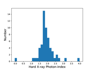
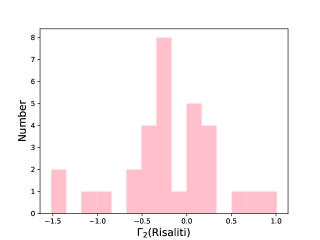
Figure 1: Top:Hard X-ray photon index derived from the fluxes collected from the XMM catalog in different X-ray bands. Bottom: UV spectral index estimated for 31 sources which satisfy the criteria of Lusso et al. (2020), i.e. that the UV spectral index should lie between $-0.7$ and 1.5.

Lusso et al. (2020) recommended a pre-selection of the sources based on criteria concerning the UV, optical/IR and X-ray slopes. We did not apply such criteria since our starting sample is already very small in comparison with their initial sample and further sample reduction is not a viable option. But we performed additional tests, apart from $\alpha_{ox}$, following the recommendations of Lusso et al. (2020). For all 58 objects, having the X-ray fluxes in several X-ray bands from 4XMMDR11 we fitted a broken power law to the data, fixing the frequency break at 1 keV rest frame, and obtained best fits for the slopes. The histogram of the hard X-ray slopes is shown in Fig. 1. Out of 58 sources, 41 satisfy the criterion that the photon index should be between 1.7 and 2.8. In the whole sample only 3 objects are very strong outliers, two with slopes extremely soft and one (NGC 4151) with a very hard slope indicating strong absorption.

We also collected the GALEX far-UV magnitudes using the GALEX EUV quasar colors catalogue of SDSS QSOs DR14 (Vanden Berk et al., 2020), but data were available only for 31 sources out of 58. Since the GALEX magnitude is a broad-band index, very sensitive to the spectral shape, we performed the estimate of the far-UV slope by using the 3000 Å rest frame flux from Table LABEL:tab_xray_uv_data, assuming an arbitrary slope for a power-law extending from 3000 Å rest frame to far-UV, correcting the spectral shape for Galactic extinction by using the value $A_{V}$ and the extinction curve from Cardelli et al. (1989), and calculated the predicted GALEX flux by folding the resulting spectrum with the profile of the GALEX far-UV filter. We thus obtained the best fit slope by matching the predicted and the measured magnitudes. Lusso et al. (2020) recommended using only sources with spectral index between $-0.7$ and 1.5 in the far-UV. A distribution of UV spectral indices of 31 sources is shown in the bottom panel of Fig. 1. Among the 31 sources for which we have the data, only 4 do not satisfy this criterion. According to Lusso et al. (2020) we should combine the two criteria. This would leave us with only 21 objects.

Finally, Lusso et al. (2020) recommend removing the Eddington bias by actually removing all outliers from the expected X-ray flux. This is done assuming a standard relation and comparing the predicted 2 keV flux with the minimum which can be detected observationally. In a single short XMM exposure they estimate the minimum flux at $4.6\times 10^{-32}$ erg s^-1 cm^-2 Hz^-1. Our fluxes are frequently lower but the reported fluxes are almost always the results of the multiple exposures, so the errors quoted in Table LABEL:tab_xray_uv_data are small and we do not believe we have problems with marginal detections. However, the reduction of the sample to 21 objects would undermine the effort of the comparison of the two methods. So we use the whole sample, and the issue can be addressed in the future when many more AGN will have reverberation measured time delays (see e.g., Czerny et al., 2023, and references therein).

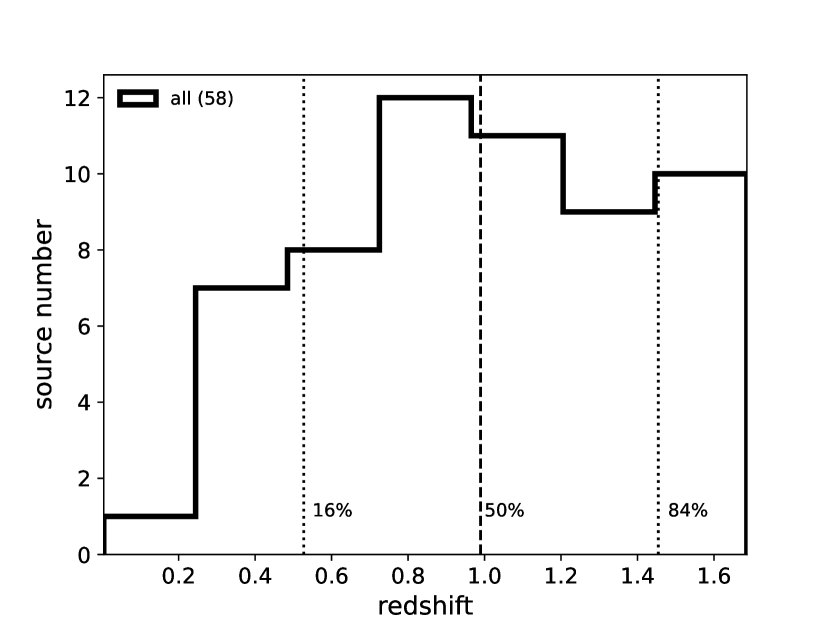
Figure 2: Redshift distribution of the QSO sample (58 sources). The vertical lines mark the percentiles as indicated (16%, 50%, 84%). The bin size is $\Delta z\simeq 0.24$ (7 bins according to Doane’s rule).

The redshift range of the X-ray/UV and ($\tau$, $F_{3000}$) sample is $0.0041\leq z\leq 1.686$, with median value of $0.990$. Except for NGC4151, peculiar velocities can be neglected. For NGC4151, the original $z=0.0033$ was corrected to $z=0.0041$ after accounting for the peculiar velocity effect. The 16%-percentile (25%-percentile) value of redshift is $0.527$ ( 0.716), while the $84\%$-percentile (75%-percentile) value is $1.454$ (1.270). The redshift distribution is displayed in Fig. 2 with bin size $\Delta z\simeq 0.24$ (7 bins) determined using Doane’s rule, which takes into account the distribution skewness.

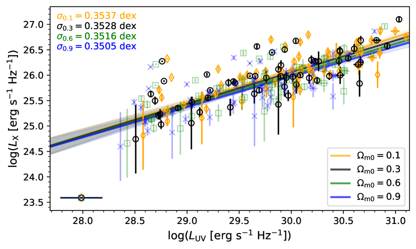
Figure 3: The correlation between 2 keV X-ray and 2500 Å UV luminosities (in ${\rm erg\,s^{-1}Hz^{-1}}$ and UV luminosities scaled to $10^{29}\,{\rm erg\,s^{-1}Hz^{-1}}$) for 58 sources. These are computed for a fixed flat $\Lambda$CDM cosmological model ($H_{0}=70\,{\rm km\,s^{-1}\,Mpc^{-1}}$) for four different values of $\Omega_{m0}$ (0.1, 0.3, 0.6, 0.9). The black solid line is the best-fit linear relation for $\Omega_{m0}=0.3$. The gray shaded area indicates $1\sigma$ uncertainties of the fit. The intrinsic RMS scatter of data points around the best-fit relation is $\sigma_{\rm ext}=0.35$ dex. The best-fit relations for $\Omega_{\rm m0}=0.1$, $\Omega_{m0}=0.6$, and $\Omega_{m0}=0.9$ are shown in orange, green, and blue, respectively.

For the cross-matched UV/X-ray sample, we determine the correlation between X-ray and UV monochromatic luminosities at 2 keV and 2500 Å, respectively, in the fixed flat $\Lambda$CDM model (with $H_{0}=70\,{\rm km\,s^{-1}\,Mpc^{-1}}$ and $\Omega_{m0}=0.3$). The correlation is positive and significant, with Pearson correlation coefficient $r=0.78$ ($p=6.54\times 10^{-13}$) and Spearman rank-order correlation coefficient $\rho=0.74$ ($p=2.90\times 10^{-11}$). When we determine the correlation coefficients from the smaller to the larger $\Omega_{m0}$, we obtain $r=0.80$ ($p=3.82\times 10^{-14}$) and $\rho=0.78$ ($p=8.31\times 10^{-13}$), $r=0.76$ ($p=5.45\times 10^{-12}$) and $\rho=0.72$ ($p=2.63\times 10^{-10}$), $r=0.75$ ($p=1.91\times 10^{-11}$) and $\rho=0.70$ ($p=7.36\times 10^{-10}$) for $\Omega_{\rm m0}=0.1$, $0.6$, and $0.9$, respectively. Hence, the correlation slightly decreases for larger values of $\Omega_{m0}$. We fit a linear function to the $L_{X}-L_{UV}$ distribution for 58 sources, neglecting $L_{\rm X}$ and $L_{\rm UV}$ uncertainties. Looking for the solution with the smallest RMS scatter we obtain,

$$\log L_{X} =(0.65\pm 0.06)\log L_{29}+(25.46\pm 0.07),\ \Omega_{m0}=0.1,$$

$$\log L_{X} =(0.63\pm 0.07)\log L_{29}+(25.43\pm 0.07),\ \Omega_{m0}=0.3,$$

$$\log L_{X} =(0.61\pm 0.07)\log L_{29}+(25.40\pm 0.07),\ \Omega_{m0}=0.6,$$

$$\log L_{X} =(0.60\pm 0.07)\log L_{29}+(25.37\pm 0.06),\ \Omega_{m0}=0.9\,,$$ (17)

where $L_{29}\equiv L_{UV}/10^{29}\,{\rm erg\,s^{-1}\,Hz^{-1}}$. The global RMS scatter around the best-fit relation is $\sigma_{\rm ext}\simeq 0.35$ dex. The X-ray/UV correlation for 58 data points and the linear fit with 1$\sigma$ uncertainties in eq. (17) are shown in Fig. 3. The best-fit coefficients in eq. (17) are overall consistent within $1\sigma$ uncertainties with the best-fit relation of Lusso & Risaliti (2016), their Fig. 3, with $\log{L_{\rm X}}=0.642^{+0.015}_{-0.005}\log{L_{\rm UV}}+6.965^{+0.461}_{-0.465}$ (for $L_{29}$ normalization, their mean value of the intercept would be $\beta=25.583$), with their dispersion being $\sigma_{\rm ext}=0.24$. High redshift quasars give the same slope, $0.60\pm 0.02$ as lower redshift sources (Sacchi et al., 2022). These results are also consistent with the more accurate results we derive from a joint determination of the $L_{X}-L_{UV}$ relation parameters and the cosmological model parameters, discussed in Sec. 5 below. In Fig. 3 we compare the eq. (17) $L_{X}-L_{UV}$ relations for four different values of $\Omega_{m0}$ (0.1, 0.3, 0.6, 0.9) using orange, black, green, and blue lines and points, respectively. The best-fit coefficients are overall consistent within $1\sigma$ uncertainties, with a mild indication of slope and intercept decrease as well as intrinsic RMS scatter decrease for higher values of $\Omega_{m0}$.

Figure 4: The correlation between rest-frame Mg ii time-delay (in days) and monochromatic luminosity at 3000 Å (in ${\rm erg\,s^{-1}}$ and scaled to $10^{44}\,{\rm erg\,s^{-1}}$) for 59 sources. These are computed for a fixed flat $\Lambda$CDM model with $H_{0}=70\,{\rm km\,s^{-1}\,Mpc^{-3}}$ and four values of $\Omega_{m0}$ (0.1, 0.3,0.6,0.9). The best-fit relation for $\Omega_{m0}=0.3$ is depicted by the black solid line, with the $1\sigma$ uncertainty range shown by the shaded gray region. The 59 data points have an intrinsic RMS scatter of $\sim 0.30$ dex around the best-fit relation. For comparison, we also show $\tau-L_{3000}$ correlations and their best-fit relations for $\Omega_{\rm m0}=0.1$, $\Omega_{m0}=0.6$, and $\Omega_{m0}=0.9$ in orange, green, and blue, respectively.

The second correlation expected for the cross-matched data set is the relation between the UV monochromatic luminosity at 3000 Å  and the rest-frame Mg ii broad-line time delay, the $R-L$ relation. This correlation is again positive and significant, with Pearson correlation coefficient $r=0.56$ ($p=4.42\times 10^{-6}$) and Spearman rank-order coefficient $\rho=0.39$ ($p=0.0024$) for flat $\Lambda$CDM cosmology with $H_{0}=70\,{\rm km\,s^{-1}\,Mpc^{-1}}$ and $\Omega_{m0}=0.3$. When going from the smaller to the higher $\Omega_{m0}$, one obtains $r=0.56$ ($p=3.63\times 10^{-6}$) and $\rho=0.39$ ($p=0.0024$), $r=0.55$ ($p=6.05\times 10^{-6}$) and $\rho=0.39$ ($p=0.0022$), and $r=0.55$ ($p=7.93\times 10^{-6}$) and $\rho=0.39$ ($p=0.0024$) for $\Omega_{m0}=0.1$, $0.6$, and $0.9$, respectively. In comparison with the X-ray/UV luminosity relation, the $R-L$ relation is generally weaker and less significant. The correlation and its significance is, however, not significantly affected by different values of $\Omega_{m0}$. When we infer the monochromatic luminosities at 3000 Å  using the fixed flat $\Lambda$CDM model with the same fixed parameters as before ($\Omega_{m0}=0.1,0.3,0.6,0.9$ and $H_{0}=70\,{\rm km\,s^{-1}\,Mpc^{-1}}$), we obtain the best-fit $R-L$ relations for the 59 sources (neglecting time-delay and luminosity uncertainties),

$$\log{\tau} =(0.27\pm 0.05)\log{L_{44}}+(1.63\pm 0.06),\ \Omega_{m0}=0.1,$$

$$\log{\tau} =(0.28\pm 0.06)\log{L_{44}}+(1.66\pm 0.06),\ \Omega_{m0}=0.3,$$

$$\log{\tau} =(0.29\pm 0.06)\log{L_{44}}+(1.68\pm 0.06),\ \Omega_{m0}=0.6,$$

$$\log{\tau} =(0.29\pm 0.06)\log{L_{44}}+(1.70\pm 0.05),\ \Omega_{m0}=0.9,$$ (18)

where $L_{44}\equiv L_{3000}/10^{44}\,{\rm erg\,s^{-1}}$ is the monochromatic luminosity at 3000 Å, $L_{3000}$, scaled to $10^{44}\,{\rm erg\,s^{-1}}$. The relations in eq. (18) with 1$\sigma$ uncertainties are depicted in Fig. 4 alongside 59 data points, which have $\sigma_{\rm ext}=0.30$ dex global RMS scatter around the best-fit relation. The best-fit coefficients in eq. (18) derived based on 59 Mg ii QSOs are, within uncertainties, consistent with the previously inferred slopes and intercepts for slightly larger Mg ii data sets (Martínez-Aldama et al., 2020; Khadka et al., 2021a, 2022b; Prince et al., 2022; Cao et al., 2022e). These results are also consistent with the more accurate results we derive from a joint determination of the $R-L$ relation parameters and the cosmological model parameters, discussed in Sec. 5 below. In Fig. 4 we compare eq. (18) $R-L$ relations for different values of $\Omega_{m0}$ (0.1, 0.3, 0.6, 0.9). While the best-fit coefficients are overall consistent within 1$\sigma$ uncertainties, we observe a mild indication of slope and intercept increasing as well as intrinsic RMS scatter increasing for higher values of $\Omega_{m0}$, i.e. the opposite trend in comparison with $L_{X}-L_{UV}$ relation for the slope and the intrinsic scatter.

Here we also use 11 BAO data points given in Table 1 of Khadka & Ratra (2021) and 31 $H(z)$ observations data points give in Table 2 of Ryan et al. (2018). We use the better-established joint BAO+$H(z)$ data set cosmological parameter constraints for comparison with the cosmological parameters constraints determined here using Mg ii $R-L$ data and Mg ii $L_{X}-L_{UV}$ data.

4 Methods

We use 58 (59) pairs of QSO measurements to constrain cosmological parameters and $L_{X}-L_{UV}$ ($R-L$) relation parameters.

In the case of the $R-L$ relation, for a given model, we predict rest-frame time-delays of QSOs at known redshift $z_{i}$ using eq. (5) and these predicted time-delays are compared with the corresponding observed time-delays using the likelihood function LF (D’Agostini, 2005)

$$\ln({\rm LF})=-\frac{1}{2}\sum^{N}_{i=1}\left[\frac{[\log(\tau^{\rm obs}_{i})-\log(\tau^{\rm th}_{i})]^{2}}{s^{2}_{i}}+\ln(2\pi s^{2}_{i})\right].$$ (19)

Here $\ln$ = $\log_{e}$, $\tau^{\rm th}_{i}(\mathbf{p})$ and $\tau^{\rm obs}_{i}$ are the predicted and observed time-delays at redshift $z_{i}$, and $s^{2}_{i}=\sigma^{2}_{\log{\tau_{\rm obs},i}}+\gamma^{2}\sigma^{2}_{\log{F_{3000},i}}+\sigma_{\rm ext}^{2}$, where $\sigma_{\log{\tau_{\rm obs},i}}$ and $\sigma_{\log{F_{3000},i}}$ are the measurement error on the observed time-delay and the measured flux ($F_{3000}$) respectively, and $\sigma_{\rm ext}$ is the global intrinsic dispersion of the $R-L$ relation.

Table 1: Summary of the non-zero flat prior parameter ranges.

Parameter	Prior range
$\Omega_{b}h^{2}$	$[0,1]$
$\Omega_{c}h^{2}$	$[0,1]$
$\Omega_{m0}$	$[0,1]$
$\Omega_{k0}$	$[-2,2]$
$\omega_{X}$	$[-5,0.33]$
$\alpha$	$[0,10]$
$\sigma_{\rm ext}$	$[0,5]$
$\beta$	$[0,10]$ for the $R-L$ relation and $[0,50]$ for the $L_{X}-L_{UV}$ relation.
$\gamma$	$[0,5]$

• Here $\Omega_{b}$ and $\Omega_{c}$ are the current values of the non-relativistic baryonic and CDM density parameters and $h$ is $H_{0}$ in units of 100 km s^-1 Mpc^-1. We use $\Omega_{b}$ and $\Omega_{c}$ as free parameters in the BAO data analyses, instead of $\Omega_{m0}=\Omega_{b}+\Omega_{c}$.

Similarly, in the case of the $L_{X}-L_{UV}$ relation, in a given model, we can predict X-ray fluxes of QSOs at known redshift $z_{i}$ using eq. (2) and these fluxes are compared with the corresponding observed X-ray fluxes using the likelihood function LF (D’Agostini, 2005)

$$\ln({\rm LF})=-\frac{1}{2}\sum^{N}_{i=1}\left[\frac{[\log(F^{\rm obs}_{X,i})-\log(F^{\rm th}_{X,i})]^{2}}{s^{2}_{i}}+\ln(2\pi s^{2}_{i})\right],$$ (20)

with $s^{2}_{i}=\sigma^{2}_{\log{F_{UV}}}+\gamma^{2}\sigma^{2}_{\log{F_{UV},i}}+\sigma_{\rm ext}^{2}$, where $\sigma^{2}_{\log{F_{UV}}}$ and $\sigma^{2}_{\log{F_{UV},i}}$ are the measurement error on the observed X-ray and UV fluxes respectively, and $\sigma_{\rm ext}$ is the global intrinsic dispersion of the $L_{X}-L_{UV}$ relation. $F^{\rm th}_{X,i}(\mathbf{p})$ is the predicted flux at redshift $z_{i}$.

We maximize the likelihood functions given in eqs. (19) and (20) by performing Markov chain Monte Carlo (MCMC) sampling implemented in the MontePython code (Brinckmann & Lesgourgues, 2019). We use flat priors on each free parameter involved in the computation and the priors we use are given in Table 1. The convergence of each chain corresponding to free parameters is confirmed by satisfying the Gelman-Rubin convergence criterion, $R-1<0.05$. Each chain obtained from the MCMC sampling is analysed using the Python package Getdist (Lewis, 2019).

We compare the performance of the $R-L$ and the $L_{X}-L_{UV}$ relations by computing the Akaike and the Bayesian information criterion ($AIC$ and $BIC$) values for each analysis. The $AIC$ and the $BIC$ values are given by

$$AIC= \chi^{2}_{\rm min}+2d,$$ (21)

$$BIC= \chi^{2}_{\rm min}+d\ln{N}\,,$$ (22)

where $\chi^{2}_{\rm min}=-2\ln({\rm LF}_{\rm max})$. Here $N$ is the number of data points, $d$ is the number of free parameters, and the number of degrees of freedom is $dof=N-d$.

Model	Data set	$\Omega_{m0}$	$\Omega_{k0}$	$\omega_{X}$	$\alpha$	$\sigma_{\rm ext}$	$\beta$a	$\gamma$b	$dof$	$-$2$\ln(LF_{\rm max})$	$AIC$	$BIC$
Flat $\Lambda$CDM	$H(z)$ + BAO	0.298	–	–	–	–	–	–	39	23.66	29.66	34.87
	$R-L$ QSOs	0.053	–	–	–	0.288	1.642	0.259	55	25.78	33.78	42.09
	$L_{X}-L_{UV}$ QSOs	0.995	–	–	–	0.329	25.393	0.599	54	44.10	52.10	60.34
Non-flat $\Lambda$CDM	$H(z)$ + BAO	0.294	0.031	–	–	–	–	–	38	23.60	31.60	38.55
	$R-L$ QSOs	0.315	$-$0.974	–	–	0.284	1.590	0.336	54	22.80	32.80	43.19
	$L_{X}-L_{UV}$ QSOs	0.986	1.987	–	–	0.329	25.355	0.587	53	42.96	52.96	63.26
Flat XCDM	$H(z)$ + BAO	0.280	–	$-$0.691	–	–	–	–	38	19.66	27.66	34.61
	$R-L$ QSOs	0.002	–	$-$4.997	–	0.278	1.343	0.215	54	19.76	29.76	40.15
	$L_{X}-L_{UV}$ QSOs	0.103	–	0.139	–	0.329	25.385	0.580	53	43.96	53.96	64.26
Non-flat XCDM	$H(z)$ + BAO	0.291	$-$0.147	$-$0.641	–	–	–	–	37	18.34	28.34	37.03
	$R-L$ QSOs	0.052	$-$0.101	$-$3.055	–	0.281	1.402	0.281	53	21.44	33.44	45.91
	$L_{X}-L_{UV}$ QSOs	0.952	1.952	$-$4.840	–	0.329	25.290	0.591	52	41.48	53.48	65.84
Flat $\phi$CDM	$H(z)$ + BAO	0.265	–	–	1.445	–	–	–	38	19.56	27.56	34.51
	$R-L$ QSOs	0.066	–	–	0.003	0.292	1.640	0.264	54	25.8	35.8	46.19
	$L_{X}-L_{UV}$ QSOs	0.997	–	–	9.105	0.331	25.399	0.596	53	44.08	54.08	64.38
Non-flat $\phi$CDM	$H(z)$ + BAO	0.261	$-$0.155	–	2.042	–	–	–	37	18.16	28.16	36.85
	$R-L$ QSOs	0.126	$-$0.124	–	0.083	0.293	1.631	0.280	53	25.8	37.8	50.27
	$L_{X}-L_{UV}$ QSOs	0.970	$-$0.919	–	9.321	0.330	25.372	0.567	52	43.94	55.94	68.30

• For $R-L$ data $\beta$ values are for the $R-L$ relation and for $L_{X}-L_{UV}$ data $\beta$ values are for the $L_{X}-L_{UV}$ relation.

• For $R-L$ data $\gamma$ values are for the $R-L$ relation and for $L_{X}-L_{UV}$ data $\gamma$ values are for the $L_{X}-L_{UV}$ relation.

Table 2: Unmarginalized best-fit parameters from all data sets.

Model	Data set	$\Omega_{m0}$	$\Omega_{k0}$	$\omega_{X}$	$\alpha$	$\sigma_{\rm ext}$	$\beta$a	$\gamma$b
Flat $\Lambda$CDM	$H(z)$ + BAO	$0.299^{+0.015}_{-0.017}$	–	–	–	–	–	–
	$R-L$ QSOs	$<0.614$ (1$\sigma$)	–	–	–	$0.305^{+0.028}_{-0.037}$	$1.681\pm 0.066$	$0.276\pm 0.061$
	$L_{X}-L_{UV}$ QSOs	$>0.407$ (1$\sigma$)	–	–	–	$0.350^{+0.033}_{-0.044}$	$25.436\pm 0.077$	$0.616\pm 0.074$
Non-flat $\Lambda$CDM	$H(z)$ + BAO	$0.292\pm 0.023$	$-0.014\pm 0.075$	–	–	–	–	–	–
	$R-L$ QSOs	$0.54^{+0.370}_{-0.220}$	$-0.200^{+0.780}_{-1.400}$	–	–	$0.304^{+0.028}_{-0.037}$	$1.677^{+0.074}_{-0.067}$	$0.290\pm 0.065$
	$L_{X}-L_{UV}$ QSOs	$>0.412$ (1$\sigma$)	$>-0.998$ (2$\sigma$)	–	–	$0.349^{+0.032}_{-0.043}$	$25.417\pm 0.076$	$0.609\pm 0.073$
Flat XCDM	$H(z)$ + BAO	$0.282\pm 0.021$	–	$-0.744^{+0.149}_{-0.097}$	–	–	–	–
	$R-L$ QSOs	$<0.513$ (1$\sigma$)	–	$<-0.390$ (2$\sigma$)	–	$0.302^{+0.028}_{-0.037}$	$1.630^{+0.120}_{-0.074}$	$0.275\pm 0.060$
	$L_{X}-L_{UV}$ QSOs	$>0.475$ (1$\sigma$)	–	$-2.100^{+2.200}_{-1.100}$	–	$0.351^{+0.033}_{-0.044}$	$25.438^{+0.073}_{-0.087}$	$0.614\pm 0.075$
Non-flat XCDM	$H(z)$ + BAO	$0.293\pm 0.027$	$-0.120\pm 0.130$	$-0.693^{+0.130}_{-0.077}$	–	–	–	–
	$R-L$ QSOs	$0.510\pm 0.270$	$-0.070^{+0.640}_{-0.970}$	$-2.400^{+1.900}_{-1.400}$	–	$0.303^{+0.028}_{-0.037}$	$1.650^{+0.110}_{-0.073}$	$0.289\pm 0.065$
	$L_{X}-L_{UV}$ QSOs	$>0.427$ (1$\sigma$)	$>0.355$ ($(2\sigma)$)	$-2.300^{+2.300}_{-1.100}$	–	$0.348^{+0.033}_{-0.044}$	$25.394^{+0.075}_{-0.085}$	$0.608\pm 0.075$
Flat $\phi$CDM	$H(z)$ + BAO	$0.266\pm 0.023$	–	–	$1.530^{+0.620}_{-0.850}$	–	–	–
	$R-L$ QSOs	–	–	–	–	$0.305^{+0.027}_{-0.037}$	$1.701\pm 0.060$	$0.280\pm 0.061$
	$L_{X}-L_{UV}$ QSOs	$0.530^{+0.420}_{-0.200}$	–	–	–	$0.349^{+0.032}_{-0.043}$	$25.419\pm 0.070$	$0.609\pm 0.073$
Non-flat $\phi$CDM	$H(z)$ + BAO	$0.271^{+0.024}_{-0.028}$	$-0.080\pm 0.100$	–	$1.660^{+0.670}_{-0.830}$	–	–	–
	$R-L$ QSOs	$0.460^{+0.180}_{-0.430}$	$0.060\pm 0.370$	–	–	$0.305^{+0.029}_{-0.037}$	$1.702\pm 0.060$	$0.280\pm 0.061$
	$L_{X}-L_{UV}$ QSOs	–	$0.030\pm 0.370$	–	$5.100^{+2.700}_{-2.700}$	$0.348^{+0.034}_{-0.044}$	$25.418\pm 0.070$	$0.610\pm 0.073$

• For $R-L$ data $\beta$ values are for the $R-L$ relation and for $L_{X}-L_{UV}$ data $\beta$ values are for the $L_{X}-L_{UV}$ relation.

• For $R-L$ data $\gamma$ values are for the $R-L$ relation and for $L_{X}-L_{UV}$ data $\gamma$ values are for the $L_{X}-L_{UV}$ relation.

Table 3: One-dimensional marginalized posterior mean values and uncertainties ($\pm 1\sigma$ error bars or $2\sigma$ limits) of the parameters for all models for all data sets.

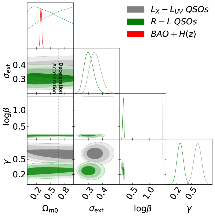
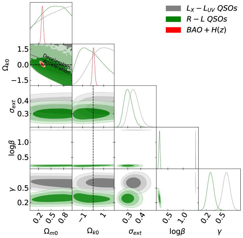
Figure 5: One-dimensional likelihood distributions and two-dimensional contours at 1$\sigma$, 2$\sigma$, and 3$\sigma$ confidence levels using $L_{X}-L_{UV}$ QSO (gray), $R-L$ QSO (green), and BAO + $H(z)$ (red) data for all free parameters. Left panel shows the flat $\Lambda$CDM model. The black dotted vertical lines are the zero acceleration lines with currently accelerated cosmological expansion occurring to the left of the lines. Right panel shows the non-flat $\Lambda$CDM model. The black dotted sloping line in the $\Omega_{k0}-\Omega_{m0}$ subpanel is the zero acceleration line with currently accelerated cosmological expansion occurring to the lower left of the line. The black dashed horizontal or vertical line in the $\Omega_{k0}$ subpanels correspond to $\Omega_{k0}=0$.

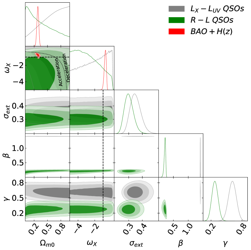
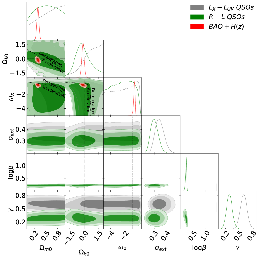
Figure 6: One-dimensional likelihood distributions and two-dimensional contours at 1$\sigma$, 2$\sigma$, and 3$\sigma$ confidence levels using $L_{X}-L_{UV}$ QSO (gray), $R-L$ QSO (green), and BAO + $H(z)$ (red) data for all free parameters. Left panel shows the flat XCDM parametrization. The black dotted curved line in the $\omega_{X}-\Omega_{m0}$ subpanel is the zero acceleration line with currently accelerated cosmological expansion occurring below the line and the black dashed straight lines correspond to the $\omega_{X}=-1$ $\Lambda$CDM model. Right panel shows the non-flat XCDM parametrization. The black dotted lines in the $\Omega_{k0}-\Omega_{m0}$, $\omega_{X}-\Omega_{m0}$, and $\omega_{X}-\Omega_{k0}$ subpanels are the zero acceleration lines with currently accelerated cosmological expansion occurring below the lines. Each of the three lines is computed with the third parameter set to the BAO + $H(z)$ data best-fit value. The black dashed straight lines correspond to the $\omega_{x}=-1$ $\Lambda$CDM model. The black dotted-dashed straight lines correspond to $\Omega_{k0}=0$.

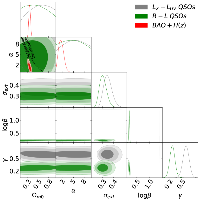
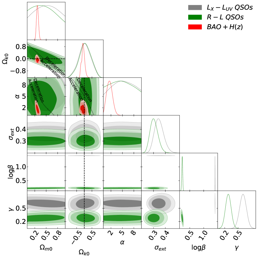
Figure 7: One-dimensional likelihood distributions and two-dimensional contours at 1$\sigma$, 2$\sigma$, and 3$\sigma$ confidence levels using $L_{X}-L_{UV}$ QSO (gray), $R-L$ QSO (green), and BAO + $H(z)$ (red) data for all free parameters. The $\alpha=0$ axes correspond to the $\Lambda$CDM model. Left panel shows the flat $\phi$CDM model. The black dotted curved line in the $\alpha-\Omega_{m0}$ subpanel is the zero acceleration line with currently accelerated cosmological expansion occurring to the left of the line. Right panel shows the non-flat $\phi$CDM model. The black dotted lines in the $\Omega_{k0}-\Omega_{m0}$, $\alpha-\Omega_{m0}$, and $\alpha-\Omega_{k0}$ subpanels are the zero acceleration lines with currently accelerated cosmological expansion occurring below the lines. Each of the three lines is computed with the third parameter set to the BAO + $H(z)$ data best-fit value. The black dashed straight lines correspond to $\Omega_{k0}=0$.

5 Results

We have compiled a QSO sample that allows us to obtain cosmological constraints from two independent methods:

• by using the Mg ii emission-line time delay with respect to the UV continuum and the resulting $R-L$ relation, and

• by using the X-ray luminosity – UV luminosity, $L_{X}-L_{UV}$, relation.

In this section, we present our results and then discuss them in two ways. First, we analyse the cosmological parameter and $R-L$ relation or $L_{X}-L_{UV}$ relation parameter constraints. We then compare the luminosity distance measurements for each source from these two independent methods.

Our cosmological parameter, $R-L$ relation parameter, and $L_{X}-L_{UV}$ relation parameter constraint results are listed in Tables 2 and 3. Unmarginalized best-fit parameters are listed in Table 2 and one-dimensional marginalized posterior mean values and corresponding uncertainties are listed in Table 3. The one-dimensional likelihoods and two-dimensional confidence contours are plotted in Figs. 5–7. $R-L$ QSO data, $L_{X}-L_{UV}$ QSO data, and BAO + $H(z)$ data results are shown in green, gray, and red. Here we have used the better-established BAO + $H(z)$ data results from Khadka & Ratra (2021) to compare with results obtained from $R-L$ QSO data and $L_{X}-L_{UV}$ QSO data. For a detailed discussion of the BAO + $H(z)$ results see Khadka & Ratra (2021).

5.1 Parameter constraint results from the two methods

In this paper we use 59 (58) pairs of QSO measurements to simultaneously constrain the cosmological parameters and the $R-L$ ($L_{X}-L_{UV}$) relation parameters in six different cosmological models.

For the $R-L$ relation, in all six models, the value of intercept $\beta$ ranges from $1.630^{+0.120}_{-0.074}$ to $1.702\pm 0.060$ and the value of slope $\gamma$ ranges from $0.275\pm 0.060$ to $0.290\pm 0.065$. For the $L_{X}-L_{UV}$ relation, in all six models, the value of intercept $\beta$ ranges from $25.417\pm 0.076$ to $25.438^{+0.073}_{-0.087}$ and the value of slope $\gamma$ ranges from $0.608\pm 0.075$ to $0.616\pm 0.074$. These $\gamma$ and $\beta$ values are almost completely model independent, indicating that these $R-L$ relation and $L_{X}-L_{UV}$ relation QSOs are standardizable. While the slope $\gamma$ for the $R-L$ relation is determined to within $\sim 22$% at 1$\sigma$, for the $L_{X}-L_{UV}$ relation $\gamma$ is better determined to within $\sim 12$% at 1$\sigma$. The intercept $\beta$ for the $R-L$ relation is determined to within $\sim 4-6$% at 1$\sigma$ and for the $L_{X}-L_{UV}$ relation $\beta$ is also better determined to within $\sim 0.3$% at 1$\sigma$.

For these QSOs the value of the intrinsic scatter $\sigma_{\rm ext}$ for $R-L$ and $L_{X}-L_{UV}$ relations are $0.302^{+0.028}_{-0.037}$–$0.305^{+0.029}_{-0.037}$ and $0.348^{+0.033}_{-0.044}$–$0.351^{+0.033}_{-0.044}$, respectively. The slightly larger value of $\sigma_{\rm ext}$ makes the $L_{X}-L_{UV}$ relation slightly less reliable than the $R-L$ relation. (An increase in the number of sources can decrease the value of $\sigma_{\rm ext}$ but this comparison is only for those sources for which both $R-L$ and $L_{X}-L_{UV}$ relations are applicable.)

These QSOs provide very weak constraints on cosmological parameters from both the $R-L$ and the $L_{X}-L_{UV}$ relation. From Table 3, using the $R-L$ relation, in all six cosmological models the value of $\Omega_{m0}$ ranges from $0.460^{+0.180}_{-0.430}$ to $<0.614$ (1$\sigma$). The minimum and maximum values correspond to the flat $\Lambda$CDM model and the non-flat $\phi$CDM model, respectively. From Table 3, using the $L_{X}-L_{UV}$ relation, in all six cosmological models the value of $\Omega_{m0}$ ranges from $>0.407$ (1$\sigma$) to $0.530^{+0.430}_{-0.200}$. The minimum and maximum values correspond to the flat $\Lambda$CDM model and the flat $\phi$CDM model, respectively. In both cases constraints on $\Omega_{m0}$ are very weak. From the plots shown in Figs. 5–7 we can see that the $\Omega_{m0}$ distributions corresponding to the $R-L$ relation have a higher probability tendency towards smaller $\Omega_{m0}$ values but $\Omega_{m0}$ distributions corresponding to the $L_{X}-L_{UV}$ relation show a higher probability tendency towards larger $\Omega_{m0}$ values. This tendency of the $L_{X}-L_{UV}$ relation is consistent with results presented in Khadka & Ratra (2021).

From Table 3, for $R-L$ data, in all three non-flat models the value of $\Omega_{k0}$ ranges from $-0.200^{+0.780}_{-1.400}$ to $0.060\pm 0.370$. For $L_{X}-L_{UV}$ data, in all three non-flat models the value of $\Omega_{k0}$ ranges from $>-0.998$ to $0.030\pm 0.370$.

From Table 3, for $R-L$ data, for the flat and non-flat XCDM parametrization the values of the equation of state parameter $\omega_{X}$ are $<-0.390$ (2$\sigma$) and $-2.400^{+1.900}_{-1.400}$, respectively. For $L_{X}-L_{UV}$ data, for the flat and non-flat XCDM parametrization the values of $\omega_{X}$ are $-2.100^{+2.200}_{-1.100}$ and $-2.300^{+2.300}_{-1.100}$, respectively. In both cases, these data provide weak constraints on $\omega_{X}$ and mostly the posterior value depends on the prior range. From Table 3, for $L_{X}-L_{UV}$ data, for the non-flat $\phi$CDM model the value of the positive parameter $\alpha$ is $5.100\pm 2.700$. These data are unable to constrain $\alpha$ in all other cases.

We have listed $AIC$ and $BIC$ values for each case in Table 2. From this table, for a given cosmological model, we see that the $AIC$ and $BIC$ values are always lower for the $R-L$ relation compared to the values for the $L_{X}-L_{UV}$ relation. This indicates that the $R-L$ relation better fits $R-L$ data than the $L_{X}-L_{UV}$ relation fits $L_{X}-L_{UV}$. This is consistent with the indications from the $\sigma_{\rm ext}$ values discussed above.

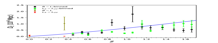
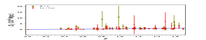
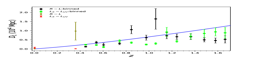
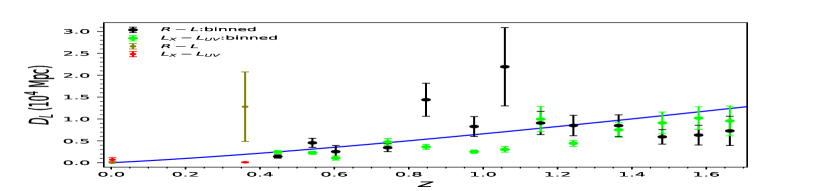
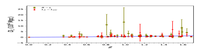
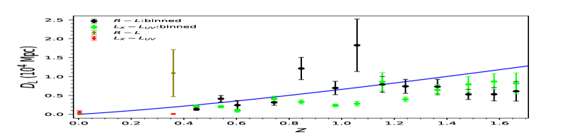
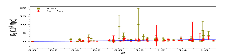
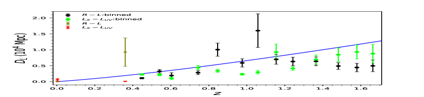
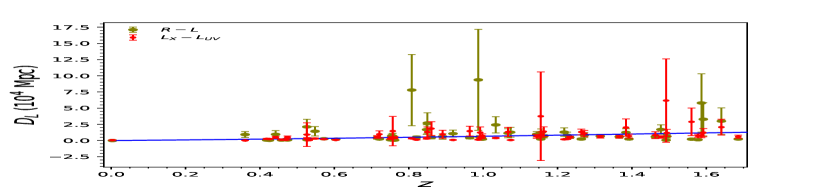
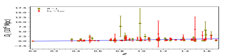
Figure 8: Comparison of individual (right column) or (largely) binned (left column) $R-L$ and $L_{X}-L_{UV}$ luminosity distances for each source in, from top row to bottom row, the flat and non-flat $\Lambda$CDM, flat and non-flat XCDM, and flat and non-flat $\phi$CDM models. Black (green) points show the weighted means and uncertainties of the $R-L$ ($L_{X}-L_{UV}$) luminosity distances in narrow redshift bins. These are plotted at the average redshift of points in the bin. Olive (red) points show the luminosity distances and uncertainties for each source obtained using the $R-L$ ($L_{X}-L_{UV}$) relation. The blue solid line in each subpanel is the prediction from the flat $\Lambda$CDM model with $\Omega_{m0}=0.3$.

5.2 Luminosity distances for individual sources from the two methods

Table 4: Statistical properties of the 58 point $(\log{D_{L,R-L}}-\log{D_{L,L_{X}-L_{UV}}})/(\sigma_{\log{D_{L,R-L}}}^{2}+\sigma_{\log{D_{L,L_{X}-L_{UV}}}}^{2})^{1/2}$ distributions for six cosmological models (see Fig. 9). From left to right the columns list models, median values, 16% and 84% percentiles, mean values, standard deviations, skewness, kurtosis, and two-sample Kolmogorov-Smirnov (KS) test statistic (comparing the cosmological model distribution to the flat $\Lambda$CDM model distribution) with the corresponding $p$-value.

Model	Median	16%	84%	Mean	Standard deviation	Skewness	Kurtosis	KS test
Flat $\Lambda$CDM	-0.138	-1.775	2.719	0.116	2.206	0.327	-0.207	0.00, $p=1.00$
Non-flat $\Lambda$CDM	-0.089	-1.686	2.822	0.171	2.199	0.325	-0.189	0.05, $p=1.00$
Flat XCDM	0.176	-1.379	2.656	0.329	2.031	0.204	-0.029	0.17, $p=0.36$
Non-flat XCDM	0.183	-1.422	2.804	0.362	2.067	0.227	-0.100	0.16, $p=0.49$
Flat $\phi$CDM	-0.193	-1.894	2.779	0.095	2.286	0.358	-0.241	0.05, $p=1.00$
Non-flat $\phi$CDM	-0.200	-1.901	2.777	0.091	2.286	0.360	-0.243	0.05, $p=1.00$

Equations (5) and (2) may be inverted to give $R-L$ and $L_{X}-L_{UV}$ luminosity distances to a source in terms of measured quantities,

$$\log D_{L,R-L}={1\over 2\gamma}\bigg{\{}\log\tau-\beta-\gamma\big{[}\log(4\pi)-44+\log F_{3000}\big{]}\bigg{\}},$$ (23)

and

$$\log D_{L,L_{X}-L_{UV}}=$$

$$\ \ {1\over 2(1-\gamma)}\bigg{[}\beta+(\gamma-1)\log(4\pi)+\gamma(\log F_{UV}-29)-\log F_{X}\bigg{]},$$ (24)

with corresponding errors derived by the first-order Taylor expansion,

$$\sigma_{\log D_{L,R-L}}=$$ (25)

$${1\over 2}\Bigg{\{}\sigma^{2}_{\log F_{3000}} +{1\over\gamma^{2}}\left[\sigma^{2}_{\log\tau}+{1\over\gamma^{2}}(\log\tau-\beta)^{2}\sigma^{2}_{\gamma}+\sigma^{2}_{\beta}\right]\Bigg{\}}^{1\over 2},$$

and

$$\sigma_{\log D_{L,L_{X}-L_{UV}}}= {1\over 2(\gamma-1)}\Bigg{[}\sigma^{2}_{\log F_{X}}+\gamma^{2}\sigma^{2}_{\log F_{UV}}+\sigma^{2}_{\beta}$$ (26)

$$\ \ +\left(\frac{\log F_{X}-\beta-\log F_{UV}+29}{1-\gamma}\right)^{2}\sigma^{2}_{\gamma}\Bigg{]}^{1\over 2}.$$

These expressions allow us to compute the $R-L$ relation and the $L_{X}-L_{UV}$ relation luminosity distances of all sources in each of the six cosmological models. For each source, $\log\tau$, $\sigma_{\log\tau}$, $\log F_{3000}$, $\sigma_{\log F_{3000}}$, $\log F_{X}$, $\sigma_{\log F_{X}}$, $\log F_{UV}$, and $\sigma_{\log F_{UV}}$ are given in Table LABEL:tab_xray_uv_data, and for each cosmological model, $\gamma$, $\sigma_{\gamma}$, $\beta$, and $\sigma_{\beta}$ are listed in Table 3.

In Fig. 8 we compare $R-L$ and $L_{X}-L_{UV}$ luminosity distances for each source. In the left panels we plot weighted mean luminosity distances at the average redhsift of the points in the bin (see, e.g., Podariu et al., 2001), in 13 redshift bins spanning $0.4\leq z\leq 1.7$ and of width $0.1$. Each bin contains at least a single source. Lower redshift data are too sparse to be binned. In the right panels we plot the two luminosity distances of each source. The left panels, especially, show that $L_{X}-L_{UV}$ distances are significantly shorter than $R-L$ distances and $\Omega_{m0}=0.3$ flat $\Lambda$CDM model distances, especially in the $0.8\lesssim z\lesssim 1.3$ range. This explains why these $L_{X}-L_{UV}$ data favour higher $\Omega_{m0}$ values than 0.3 and higher than those favoured by these $R-L$ data. These results are similar to those of Lusso et al. (2020) and Khadka & Ratra (2021, 2022). However the causes in the two cases might not be similar as Khadka & Ratra (2021, 2022) showed that the Lusso et al. (2020) $L_{X}-L_{UV}$ sources are not standardizable, which is not the case with the $L_{X}-L_{UV}$ sources we study here. The plots of individual distances (Fig.8, right panel) show that some of the $R-L$ and $L_{X}-L_{UV}$ luminosity distance measurements have large errors and some have large offsets from the overall trends. However, simple selective removal of such sources can introduce a bias in the sample.

To better understand these systematic differences between the two luminosity distances for each source, we study distributions of $(\log{D_{L,R-L}}-\log{D_{L,L_{X}-L_{UV}}})/(\sigma_{\log{D_{L,R-L}}}^{2}+\sigma_{\log{D_{L,L_{X}-L_{UV}}}}^{2})^{1/2}$, i.e. histograms of the logarithm of the ratio $D_{L,R-L}/D_{L,L_{X}-L_{UV}}$ normalized by the combined uncertainty of the two luminosity distances for each source, where we discard the second $R-L$ distance measurement for NGC 4151. We study these distributions for the flat and non-flat $\Lambda$CDM, XCDM, and $\phi$CDM models, i.e. a total of six histograms that are shown in Fig. 9. The histograms are constructed uniformly for the six cases, with 10 equal-sized bins in the range $(-6,6)$ with bin width 1.2. The basic statistical properties of the 58 point distributions of normalized luminosity-distance differences, including the median and mean values as well as skewness and kurtosis coefficients among other things, are summarized in Table 4. The minimum and maximum median values are $-0.200$ and 0.183, respectively, corresponding to non-flat $\phi$CDM and non-flat XCDM, respectively. The minimum and maximum 16% percentile values are $-1.901$ and $-1.379$, respectively, corresponding to non-flat $\phi$CDM and flat XCDM, respectively. The 84% percentile value is in the range from $2.656$ to $2.822$, which correspond to flat XCDM and non-flat $\Lambda$CDM, respectively. The mean normalized luminosity-distance difference values have a minimum of $0.091$ for the non-flat $\phi$CDM model and a maximum of $0.362$ for the non-flat XCDM model. The standard deviation values are in the range from $2.031$ to $2.286$ corresponding to flat XCDM and flat and non-flat $\phi$CDM, respectively. The skewness coefficient has a minimum of $0.204$ for the flat XCDM model and a maximum of $0.360$ for the non-flat $\phi$CDM model. The minimum and maximum kurtosis values are $-0.243$ and $-0.029$, respectively, which correspond to the non-flat $\phi$CDM model and to the flat XCDM model, respectively. Overall, for all six cosmological models, the distributions have a positive mean value, are positively skewed, and have a negative kurtosis, which indicates that for the current limited sample of 58 sources the $R-L$ relation has a tendency to yield larger luminosity distances in comparison with the $L_{X}-L_{UV}$ relation. The negative kurtosis indicates that distribution outliers are suppressed in comparison with the normal distribution and the median value is slightly negative for all models except for flat and non-flat XCDM. The normalized luminosity-distance difference distributions for all the six cosmological models are consistent with being drawn from the same distribution, which is shown by the two-sample Kolmogorov-Smirnov (KS) test statistic calculated between a given 58 point distribution and the distribution corresponding to the flat $\Lambda$CDM model, see Table 4 (last column). The KS statistic is in the range 0.05-0.17 (excluding the comparison of the flat $\Lambda$CDM distribution with itself), with the $p$-value in the range $0.36-1.00$, hence the null hypothesis that an underlying distribution of a given normalized $D_{L}$ difference distribution and the underlying distribution corresponding to the flat $\Lambda$CDM case are identical is confirmed for all the models.

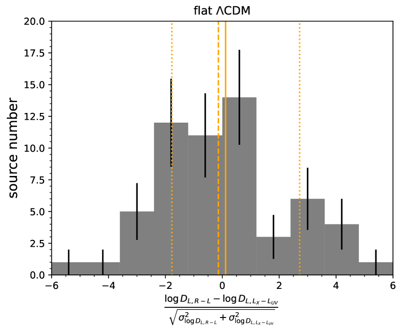
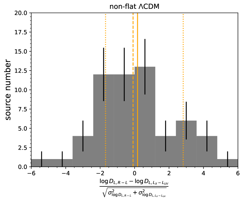
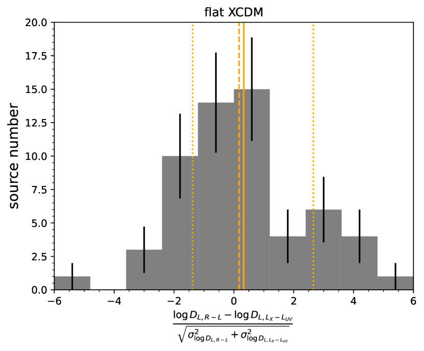
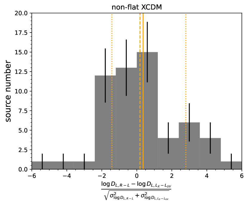
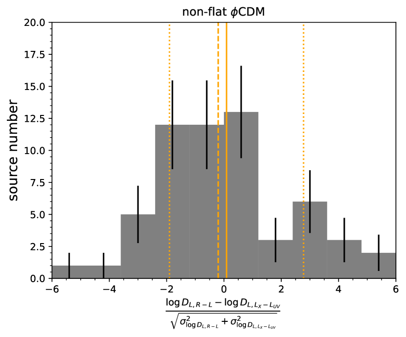
Figure 9: Histograms of $(\log{D_{L,R-L}}-\log{D_{L,L_{X}-L_{UV}}})/(\sigma_{\log{D_{L,R-L}}}^{2}+\sigma_{\log{D_{L,L_{X}-L_{UV}}}}^{2})^{1/2}$ for 58 sources in the flat and non-flat $\Lambda$CDM, XCDM, and $\phi$CDM cosmological models (from the top to the bottom). The solid vertical line stands for the distribution mean, dashed vertical line for the median, and dotted vertical lines stand for 16% and 84% percentiles. The bin size is 1.2 for all the cases (10 bins between $-6$ and 6). The uncertainties for each bin were calculated as $\sigma_{i}=\sqrt{N_{i}}$ where $N_{i}$ is the number of sources that belong to the given bin.

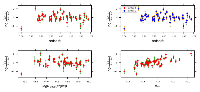
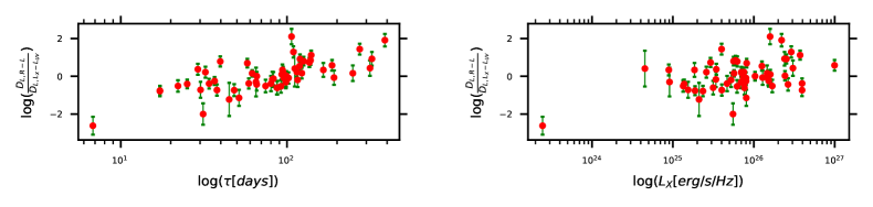
Figure 10: Ratio of $R-L$ and $L_{X}-L_{UV}$ source luminosity distances as a function of redshift, with red (blue) points in the upper left (right) panel based on method-1 (method-2). Middle panels show method-1 distance ratios as a function of source absolute luminosity at 3000 Å (middle left panel) and as a function of the $\alpha_{OX}$ parameter (middle right panel). Bottom panels show method-1 distance ratios as a function of the time delay (bottom left panel) and as a function of the source X-ray absolute luminosity.

Next we analyze differences between the $R-L$ and $L_{X}-L_{UV}$ luminosity distances for each source in the fixed $\Omega_{m0}=0.3$ flat $\Lambda$CDM model using the slope and intercept values given in eqs. (17) and (18), again discarding the second time-delay distance measurement to NGC 4151. The resulting ratios of the $R-L$ and $L_{X}-L_{UV}$ luminosity distances, $\log{(D_{L,R-L}/D_{L,L_{X}-L_{UV}})}$, are plotted as a function of $z$ in Fig. 10 using red points. [We call this technique, based on eqs. (17) and (18), "method-1".] The dispersion in the measured ratios is large, necessitating the use of the log scale: the smallest ratio is $2.4\times 10^{-3}$, for NGC 4151, while the largest ratio is 126, for object No. 160 from Homayouni et al. (2020). Half of the sources have a ratio lower than 1 (30 out of 58), and the average value of the logarithm of the ratio is $1.14\times 10^{-3}$, corresponding to a mean factor of 1.002. This indication that $L_{X}-L_{UV}$ distances on average are shorter than $R-L$ distances is qualitatively consistent with the results from the histogram in the upper left panel of Fig. 9 that fully accounts for all uncertainties (and so is more accurate than the method-1 technique result).

If instead of the fixed $\Omega_{m0}=0.3$ flat $\Lambda$CDM model slope and intercept values given in eqs. (17) and (18) we use the flat $\Lambda$CDM model coefficients from Table 3 for the correlation coefficients, i.e. we allow for different $R-L$ and $L_{X}-L_{UV}$ cosmological models and also account for the uncertainties in more parameters, we find the results shown in the top right panel of Fig. 10 using blue points. (We call this technique, based on Table 3 values, "method-2".) In this case the same number of sources have a ratio below unity, but the mean value of the logarithm of the ratio is $-0.01$, corresponding to a mean factor of 0.98, i.e. $\sim 2\%$ offset in the opposite direction, with $R-L$ placing sources closer by than $L_{X}-L_{UV}$. While differing from the result of Table 4, which indicates that $L_{X}-L_{UV}$ places sources closer by than does $R-L$, the Table 4 result is the more correct one as it accounts for the error bars of the two luminosity distances for each source, while method-2 does not account for these.

Table 5: Pearson correlation coefficients (PCC) and Spearman rank-order correlation coefficients (SCC) with the corresponding $p$-values of the distance ratio trends of Fig. 10 . All ratios are calculated for the fixed flat $\Lambda$CDM model with $\Omega_{m0}=0.3$, except for $\log{(D_{L,R-L}/D_{L,L_{X}-L_{UV}}},z)$ in the second row which is computed for the flat $\Lambda$CDM model values taken from Table 3.

Correlation	PCC	$p$-value	SCC	$p$-value	plot position
$\log{(D_{L,R-L}/D_{L,L_{X}-L_{UV}})}$, $z$	$-0.0126$	0.925	$-0.0349$	0.795	upper left panel
$\log{(D_{L,R-L}/D_{L,L_{X}-L_{UV}})}$, $z$	$6.75\times 10^{-5}$	$1.000$	$-0.0235$	0.861	upper right panel
$\log{(D_{L,R-L}/D_{L,L_{X}-L_{UV}})}$, $\log{L_{3000}}$	$-0.0698$	0.603	$-0.160$	0.232	middle left panel
$\log{(D_{L,R-L}/D_{L,L_{X}-L_{UV}})}$, $\alpha_{OX}$	0.679	$4.80\times 10^{-9}$	0.593	$9.15\times 10^{-7}$	middle right panel
$\log{(D_{L,R-L}/D_{L,L_{X}-L_{UV}})}$, $\log{\tau}$	0.686	$2.75\times 10^{-9}$	$0.707$	$5.62\times 10^{-10}$	bottom left panel
$\log{(D_{L,R-L}/D_{L,L_{X}-L_{UV}})}$, $\log{L_{X}}$	0.444	$4.84\times 10^{-4}$	0.304	$0.0204$	bottom right panel

The most extreme $D_{L}$ ratio outliers are due to the unfortunate coincidence of a short distance value from one technique and a long distance value from the other. Most of the $R-L$ and $L_{X}-L_{UV}$ source luminosity distances (107 out of 116 measurements) are within one order of magnitude from the predicted distances in the $\Omega_{m0}=0.3$ flat $\Lambda$CDM model.

However, there is no simple way of pre-selecting better measured sources to include in our sample. For example, the distance to NGC 4151 is a major problem. According to the $\Omega_{m0}=0.3$ flat $\Lambda$CDM model, it should be at 14.15 Mpc while the $R-L$ relation and the $L_{X}-L_{UV}$ relation give the values $1.59\pm 1.59$ Mpc and $698\pm 455$ Mpc, respectively (from the complete flat $\Lambda$CDM model analysis). The problem is that NGC 4151 is heavily absorbed at 3000 Å rendering the $R-L$ distance to NGC 4151 unreliable. It is also heavily absorbed in the X-ray band (e.g. de Rosa et al., 2007) and in the UV band, so the index $\alpha_{OX}$ seems typical while both measured fluxes (UV and X-ray) do not represent the intrinsic properties of the source as the source does not seem to posses the usual Big Blue Bump (Dermer & Gehrels, 1995). This is confirmed by the latest studies of the spectrum decomposition for this source by Mahmoud & Done (2020).

We searched the NED database for independent measurements of distances for all the sources in our sample. Unfortunately, except for NGC 4151, all other sources only have the $R-L$ and $L_{X}-L_{UV}$ luminosity distance measurements that we have used. Only the NGC 4151 distance has been measured using other techniques, such as the Tip of the Red Giant Branch (TRGB) (14.20 $\pm$ 0.88 Mpc, Tikhonov & Galazutdinova 2021), and the Cepheid period-luminosity relation (15.8 $\pm$ 0.4 Mpc, Yuan et al. 2020).

We also explored the potential of selecting a more reliable subsample of these sources by using only those sources whose $R-L$ and $L_{X}-L_{UV}$ luminosity distances differ by less than a factor of 3 (there are 30 such sources). For the fixed values of $\beta$ and $\gamma$ in the $R-L$ relation in eq. (18) we find from these 30 sources the constraint $\Omega_{m0}=0.4^{+0.4}_{-0.2}$ in the flat $\Lambda$CDM model. (Note that this constraint does not fully account for all the uncertainties.) This might be an interesting option in the future when there are more sources with the required measurements for both distance measurement techniques to be applicable, although it is based on the assumption that both the $R-L$ and $L_{X}-L_{UV}$ relations hold for the data set being used for this purpose and as of now this is an open question for the $L_{X}-L_{UV}$ case, for both the data set we consider here as well as for the Lusso et al. (2020) data set (see Khadka & Ratra 2021, 2022).

In the bottom four panels of Fig. 10 we also plot method-1 ratios of the $R-L$ and $L_{X}-L_{UV}$ luminosity distances, $\log{(D_{L,R-L}/D_{L,L_{X}-L_{UV}})}$, as functions of $L_{3000}$, $\alpha_{OX}$, $\tau$, and $L_{X}$, with red points. The $L_{3000}$, $\alpha_{OX}$, $\tau$, and $L_{X}$ error bars are not shown in these panels. Two systematic trends are visible in these plots. In the middle right panel of Fig. 10, we see a dependence of the distance ratio on the broad-band $\alpha_{OX}$ index. The overall trend reflects the fact that $\alpha_{OX}$ is a function of $L_{UV}$, $\alpha_{OX}\propto 0.384(1-\gamma)\log L_{UV}$. However, a significant departure of QSOs from this expected correlation also affects the luminosity distance estimation. In addition, we do not see strong correlation with the X-ray luminosity but the correlation with the time delay is again significant.

We also examine and record the quality of the correlations between the distance ratios and the other quantities shown in Fig. 10. The Pearson as well as Spearman rank-order correlation coefficients and the corresponding $p$-values for the presented relations are listed in Table 5. The significant correlations are between the distance ratio and $\alpha_{OX}$ as well as the rest-frame time delay, which are both positive. The mildly significant correlation between the distance ratio and the X-ray luminosity $L_{X}$ is positive as well. These correlations are partially driven by the fact that the luminosity distance ratio depends on $\log{F_{X}}$ and $\log{\tau}$, see eqs. (23) and (24), and the $\alpha_{OX}$ parameter depends again on $\log{F_{X}}$, see eq. (16), hence there is an intrinsic dependence that enhances the correlation. This can explicitly be inferred by evaluating $\log{(D_{L,R-L}/D_{L,L_{X}-L_{UV}})}$ using Eqs. (23) and (24),

$$\log {\left(\frac{D_{L,R-L}}{D_{L,L_{X}-L_{UV}}}\right)}$$ (27)

$$\simeq\frac{\log{\tau}}{2\gamma}-\frac{\log{F_{UV}}}{2(1-\gamma^{\prime})}+\frac{\log{F_{X}}}{2(1-\gamma^{\prime})}+C(\gamma,\beta,\gamma^{\prime},\beta^{\prime})$$

where $\gamma$ and $\beta$ are the slope and the intercept of the $R-L$ relation and $\gamma^{\prime}$ and $\beta^{\prime}$ are the slope and the intercept of the $L_{X}-L_{UV}$ relation. Hence $C(\gamma,\beta,\gamma^{\prime},\beta^{\prime})$ denotes the function of these parameters. In Eq. (5.2) we considered $F_{3000}\approx F_{\rm UV}$ for simplicity. Using the approximate values for the slopes, $\gamma\sim 0.3$ and $\gamma^{\prime}\sim 0.6$, using Eq. (16) for $\alpha_{OX}$, and using the $R-L$ relation, we can numerically evaluate Eq. (5.2),

$$\log{\left(\frac{D_{L,R-L}}{D_{L,L_{X}-L_{UV}}}\right)} \approx 1.67\log{\tau}-1.25\log{F_{UV}}+1.25\log{F_{X}}+C\,$$

$$\approx 1.67\log\tau+3.256\alpha_{OX}+C\,$$

$$\approx-0.75\log{F_{\rm UV}}+1.25\log{F_{\rm X}}+C^{\prime}\,,$$ (28)

which implies strong dependence of the luminosity distance ratio on $\tau$ and $\alpha_{OX}$ (and proportionally on $L_{X}\propto F_{\rm X}$) while at the same time there is a weaker and negative correlation with the UV flux/luminosity. This is in accordance with the correlation coefficients listed in Table 5. Taking this into account, the redshift as such is explicitly not present in the luminosity distance ratio, hence the missing correlation implies that there is no significant systematic effect with redshift for our current sample. The correlations among all the quantities should be further evaluated when the sample size increases since then some of the systematic effects may be more apparent on top of the expected intrinsically driven correlations.

6 Conclusions

Given that the previous large Lusso et al. (2020) $L_{X}-L_{UV}$ QSO data set that includes 2036 (better) QSOs that span $0.009\leq z\leq 7.5413$ is not standardizable (see Khadka & Ratra 2021, 2022), our hope here was to compile a new set of such QSOs to investigate the prospects and potential of using $L_{X}-L_{UV}$ QSO data to constrain cosmological parameters

To this end, we have compiled a small set of 58 QSOs, that span a smaller redshift range $0.0041\leq z\leq 1.686$, but with both $(\tau,F_{3000})$ and $(F_{X},F_{UV})$ data, that allow us to test both the $R-L$ and $L_{X}-L_{UV}$ relations, to compare these relations, and use these relations to jointly constrain both $R-L$ or $L_{X}-L_{UV}$ relation parameters and cosmological model parameters.

We have shown that the $R-L$ relation and $L_{X}-L_{UV}$ relation $\gamma$ and $\beta$ values are almost completely independent of cosmological model, indicating that these $R-L$ relation and $L_{X}-L_{UV}$ relation QSOs are standardizable.

While the slope, $\gamma$, and intercept, $\beta$, values are significantly better determined for the $L_{X}-L_{UV}$ data set, the slightly larger value of $\sigma_{\rm ext}$ makes the $L_{X}-L_{UV}$ data set slightly less reliable than the $R-L$ data set. However, both these data sets are small and both provide very weak constraints on cosmological parameters, with the $R-L$ relation cosmological constraints being slightly more restrictive (see Table 3 and Figs. 5–7), possibly because of the smaller value of $\sigma_{\rm ext}$.

More importantly, if we look at the trend in the $\Omega_{m0}$ posterior distributions, the $R-L$ relation ones favour lower values of $\Omega_{m0}$ compared to the $L_{X}-L_{UV}$ relation posterior distributions. This is supported by the results shown in Fig. 8 where we compare $R-L$ and $L_{X}-L_{UV}$ luminosity distances for each source (also see Fig. 9 and the related discussion), which show that $L_{X}-L_{UV}$ relation luminosity distances are significantly shorter than $R-L$ distances and $\Omega_{m0}=0.3$ flat $\Lambda$CDM model distances, especially in the $0.8\lesssim z\lesssim 1.3$ range. This explains why $L_{X}-L_{UV}$ data favour higher $\Omega_{m0}$ values than 0.3 and higher $\Omega_{m0}$ values than those favoured by $R-L$ data. While there are no independent distance measurements for any of the sources besides NGC 4151 (which is not a good $R-L$ or $L_{X}-L_{UV}$ source), Mg ii and C iv $R-L$ sources are standardizable and provide cosmological constraints consistent with those from better-established data (Khadka et al., 2021a, 2022b; Cao et al., 2022e; Cao & Ratra, 2022, 2023; Czerny et al., 2022). Consequently, more work is needed to determine whether the $L_{X}-L_{UV}$ relation can be used to standardize QSOs.

Data Availability

Data used in this paper are listed in App. A.

Appendix A X-ray detected Mg ii QSOs

Table 6: Sample of 58 X-ray detected reverberation-mapped Mg ii QSOs. From left to right, the columns stand for object ID, redshift, 2 keV X-ray flux density per frequency, 2500 Å UV flux density per frequency, 3000 Å UV flux density, Mg ii broad-line rest-frame time delay, the spectral slope between 2 keV and 2500 Å, (using the convention $F_{\nu}\propto\nu^{+\alpha_{OX}}$), and the original reference. For the Mg ii radius-luminosity analysis we consider two Mg ii time-delay determinations for NGC 4151, hence the total number of $R-L$ measurements is 59. Reference notations stand for: (a) Homayouni et al. (2020) (object IDs stand for RMIDs from the original catalogue), (b) Shen et al. (2016), (c) Shen et al. (2019), (d) Metzroth et al. (2006), and (e) Yu et al. (2021).

Object	$z$	$\log\left(\frac{F_{X}}{{\rm erg\,s^{-1}\,cm^{-2}\,Hz^{-1}}}\right)$	$\log\left(\frac{F_{UV}}{{\rm erg\,s^{-1}\,cm^{-2}\,Hz^{-1}}}\right)$	$\log\left(\frac{F_{\rm 3000}}{{\rm erg\,s^{-1}\,cm^{-2}}}\right)$	$\frac{\tau}{{\rm days}}$	$\alpha_{\rm OX}$	Ref.
18	0.8480	$-31.6897\pm 0.0764$	$-28.1437\pm 0.0012$	$-13.1079\pm 0.0009$	$125.9^{+6.8}_{-7.0}$	$-1.36\pm 0.03$	(a)
28	1.3920	$-31.5542\pm 0.0961$	$-27.4696\pm 0.0009$	$-12.4342\pm 0.0004$	$65.7^{+24.8}_{-14.2}$	$-1.57\pm 0.04$	(a)
44	1.2330	$-31.8278\pm 0.0707$	$-28.0663\pm 0.0015$	$-13.0287\pm 0.0013$	$65.8^{+18.8}_{-4.8}$	$-1.44\pm 0.03$	(a)
102	0.8610	$-31.9586\pm 0.1101$	$-27.5864\pm 0.0009$	$-12.5513\pm 0.0005$	$86.9^{+16.2}_{-13.3}$	$-1.68\pm 0.04$	(a)
114	1.2260	$-30.8388\pm 0.0438$	$-26.9031\pm 0.0008$	$-11.8697\pm 0.0003$	$186.6^{+20.3}_{-15.4}$	$-1.51\pm 0.02$	(a)
118	0.7150	$-31.3581\pm 0.0508$	$-27.2730\pm 0.0010$	$-12.2373\pm 0.0006$	$102.2^{+27.0}_{-19.5}$	$-1.57\pm 0.02$	(a)
123	0.8910	$-31.9610\pm 0.1903$	$-27.9488\pm 0.0012$	$-12.9136\pm 0.0009$	$81.6^{+28.0}_{-26.6}$	$-1.54\pm 0.07$	(a)
135	1.3150	$-31.7104\pm 0.0859$	$-27.8191\pm 0.0009$	$-12.7852\pm 0.0005$	$93.0^{+9.6}_{-9.8}$	$-1.49\pm 0.03$	(a)
158	1.4780	$-31.9433\pm 0.0986$	$-28.2366\pm 0.0014$	$-13.2007\pm 0.0012$	$119.1^{+4.0}_{-11.8}$	$-1.42\pm 0.04$	(a)
159	1.5870	$-31.7435\pm 0.0961$	$-27.7467\pm 0.0010$	$-12.7122\pm 0.0006$	$324.2^{+25.3}_{-19.4}$	$-1.53\pm 0.04$	(a)
160	0.3600	$-30.3706\pm 0.0146$	$-27.8833\pm 0.0015$	$-12.8477\pm 0.0013$	$106.5^{+18.2}_{-16.6}$	$-0.95\pm 0.01$	(a)
170	1.1630	$-31.9355\pm 0.1140$	$-27.7081\pm 0.0009$	$-12.6716\pm 0.0005$	$98.5^{+6.7}_{-17.7}$	$-1.62\pm 0.04$	(a)
185	0.9870	$-31.2580\pm 0.0179$	$-27.8888\pm 0.0094$	$-12.8508\pm 0.0093$	$387.9^{+3.3}_{-3.0}$	$-1.29\pm 0.01$	(a)
191	0.4420	$-31.8241\pm 0.0899$	$-28.1033\pm 0.0014$	$-13.0675\pm 0.0012$	$93.9^{+24.3}_{-29.1}$	$-1.43\pm 0.03$	(a)
228	1.2640	$-32.2662\pm 0.0542$	$-28.2778\pm 0.0014$	$-13.2426\pm 0.0011$	$37.9^{+14.4}_{-9.1}$	$-1.53\pm 0.02$	(a)
232	0.8080	$-31.7874\pm 0.0308$	$-28.2676\pm 0.0016$	$-13.2314\pm 0.0014$	$273.8^{+5.1}_{-4.1}$	$-1.35\pm 0.01$	(a)
240	0.7620	$-31.9561\pm 0.1068$	$-28.3802\pm 0.0022$	$-13.3449\pm 0.0021$	$17.2^{+3.5}_{-2.8}$	$-1.37\pm 0.04$	(a)
260	0.9950	$-31.4365\pm 0.0640$	$-27.4848\pm 0.0009$	$-12.4498\pm 0.0004$	$94.9^{+18.7}_{-17.2}$	$-1.52\pm 0.02$	(a)
280	1.3660	$-31.5705\pm 0.0752$	$-27.5878\pm 0.0009$	$-12.5528\pm 0.0003$	$99.1^{+3.3}_{-9.5}$	$-1.53\pm 0.03$	(a)
285	1.0340	$-31.8776\pm 0.0473$	$-28.3083\pm 0.0022$	$-13.2725\pm 0.0020$	$138.5^{+15.2}_{-21.1}$	$-1.37\pm 0.02$	(a)
291	0.5320	$-31.1633\pm 0.0174$	$-28.2683\pm 0.0018$	$-13.2328\pm 0.0016$	$39.7^{+4.2}_{-2.6}$	$-1.11\pm 0.01$	(a)
301	0.5480	$-31.5231\pm 0.0643$	$-27.8778\pm 0.0013$	$-12.8416\pm 0.0011$	$136.3^{+17.0}_{-16.9}$	$-1.40\pm 0.02$	(a)
303	0.8210	$-31.4942\pm 0.0340$	$-28.3158\pm 0.0016$	$-13.2807\pm 0.0014$	$57.7^{+10.5}_{-8.3}$	$-1.22\pm 0.01$	(a)
329	0.7210	$-31.3856\pm 0.0767$	$-27.0036\pm 0.0011$	$-11.9706\pm 0.0007$	$87.5^{+23.8}_{-14.0}$	$-1.68\pm 0.03$	(a)
338	0.4180	$-31.5911\pm 0.0768$	$-28.0706\pm 0.0015$	$-13.0372\pm 0.0013$	$22.1^{+8.8}_{-6.2}$	$-1.35\pm 0.03$	(a)
419	1.2720	$-32.0069\pm 0.0993$	$-27.9619\pm 0.0014$	$-12.9281\pm 0.0011$	$95.5^{+15.2}_{-15.5}$	$-1.55\pm 0.04$	(a)
422	1.0740	$-31.2296\pm 0.0440$	$-28.1245\pm 0.0014$	$-13.0888\pm 0.0011$	$109.3^{+25.4}_{-29.6}$	$-1.19\pm 0.02$	(a)
440	0.7540	$-31.4390\pm 0.0669$	$-27.5181\pm 0.0009$	$-12.4815\pm 0.0004$	$114.6^{+7.4}_{-10.8}$	$-1.50\pm 0.03$	(a)
449	1.2180	$-31.4268\pm 0.0489$	$-27.9928\pm 0.0015$	$-12.9586\pm 0.0013$	$119.8^{+14.7}_{-24.4}$	$-1.32\pm 0.02$	(a)
459	1.1560	$-31.9226\pm 0.1129$	$-27.9208\pm 0.0013$	$-12.8861\pm 0.0011$	$122.8^{+5.1}_{-5.7}$	$-1.54\pm 0.04$	(a)
492	0.9640	$-31.7830\pm 0.0715$	$-27.4308\pm 0.0009$	$-12.3947\pm 0.0004$	$92.0^{+16.3}_{-12.7}$	$-1.67\pm 0.03$	(a)
493	1.5920	$-31.6431\pm 0.0721$	$-27.2967\pm 0.0009$	$-12.2612\pm 0.0004$	$315.6^{+30.7}_{-35.7}$	$-1.67\pm 0.03$	(a)
501	1.1550	$-32.4490\pm 0.5935$	$-27.9964\pm 0.0012$	$-12.9586\pm 0.0009$	$44.9^{+11.7}_{-10.4}$	$-1.71\pm 0.15$	(a)
505	1.1440	$-31.9151\pm 0.1309$	$-28.1019\pm 0.0014$	$-13.0665\pm 0.0011$	$94.7^{+10.8}_{-16.7}$	$-1.46\pm 0.05$	(a)
522	1.3840	$-32.2515\pm 0.1738$	$-28.0185\pm 0.0010$	$-12.9830\pm 0.0006$	$115.8^{+11.3}_{-16.0}$	$-1.62\pm 0.06$	(a)
556	1.4940	$-31.8709\pm 0.0928$	$-27.6918\pm 0.0009$	$-12.6556\pm 0.0005$	$98.7^{+13.9}_{-10.8}$	$-1.60\pm 0.04$	(a)
588	0.9980	$-31.3856\pm 0.0604$	$-27.1696\pm 0.0008$	$-12.1343\pm 0.0002$	$74.3^{+23.0}_{-18.2}$	$-1.62\pm 0.02$	(a)
593	0.9920	$-31.9378\pm 0.1941$	$-27.7738\pm 0.0010$	$-12.7375\pm 0.0006$	$80.1^{+21.4}_{-20.8}$	$-1.60\pm 0.07$	(a)
622	0.5720	$-31.2762\pm 0.0372$	$-27.6625\pm 0.0009$	$-12.6271\pm 0.0005$	$61.7^{+6.0}_{-4.3}$	$-1.39\pm 0.01$	(a)
645	0.4740	$-31.6551\pm 0.0970$	$-27.8050\pm 0.0012$	$-12.7696\pm 0.0009$	$30.2^{+26.8}_{-8.9}$	$-1.48\pm 0.04$	(a)
649	0.8500	$-32.1753\pm 0.1679$	$-28.1288\pm 0.0015$	$-13.0931\pm 0.0013$	$165.5^{+22.2}_{-25.1}$	$-1.55\pm 0.06$	(a)
675	0.9190	$-30.9529\pm 0.0389$	$-27.5836\pm 0.0009$	$-12.5482\pm 0.0005$	$139.8^{+12.0}_{-22.6}$	$-1.29\pm 0.01$	(a)
678	1.4630	$-31.8552\pm 0.1940$	$-27.8643\pm 0.0010$	$-12.8297\pm 0.0007$	$82.9^{+11.9}_{-10.2}$	$-1.53\pm 0.07$	(a)
771	1.4920	$-32.3116\pm 0.2587$	$-27.4926\pm 0.0009$	$-12.4572\pm 0.0004$	$31.3^{+8.1}_{-4.6}$	$-1.85\pm 0.09$	(a)
774	1.6860	$-31.5946\pm 0.0877$	$-27.6123\pm 0.0009$	$-12.5768\pm 0.0004$	$58.9^{+13.7}_{-10.1}$	$-1.53\pm 0.03$	(a)
792	0.5260	$-32.2935\pm 0.6754$	$-28.5277\pm 0.0030$	$-13.4921\pm 0.0030$	$111.4^{+29.5}_{-20.0}$	$-1.45\pm 0.15$	(a)
848	0.7570	$-32.3623\pm 0.5161$	$-28.3785\pm 0.0017$	$-13.3429\pm 0.0015$	$65.1^{+29.4}_{-16.3}$	$-1.53\pm 0.20$	(a)
J141214	0.4581	$-30.9049\pm 0.0278$	$-27.2882\pm 0.0009$	$-12.2526\pm 0.0004$	$36.7^{+10.4}_{-4.8}$	$-1.39\pm 0.01$	(b), (c)
J141018	0.4696	$-31.4197\pm 0.0797$	$-28.2237\pm 0.0052$	$-13.1884\pm 0.0051$	$32.3^{+12.9}_{-5.3}$	$-1.23\pm 0.03$	(b), (c)
J141417	0.6037	$-31.5509\pm 0.0656$	$-28.5277\pm 0.0030$	$-13.4921\pm 0.0029$	$29.1^{+3.6}_{-8.8}$	$-1.16\pm 0.03$	(b), (c)
J142049	0.7510	$-31.4316\pm 0.0665$	$-27.7570\pm 0.0012$	$-12.7212\pm 0.0009$	$34.0^{+6.7}_{-12.0}$	$-1.41\pm 0.03$	(b), (c)
J141650	0.5266	$-31.8094\pm 0.1051$	$-28.2946\pm 0.0022$	$-13.2588\pm 0.0020$	$25.1^{+2.0}_{-2.6}$	$-1.35\pm 0.04$	(b), (c)
J141644	0.4253	$-31.4618\pm 0.0554$	$-27.9031\pm 0.0013$	$-12.8665\pm 0.0010$	$17.2^{+2.7}_{-2.7}$	$-1.37\pm 0.02$	(b), (c)
NGC4151	0.0041	$-28.9908\pm 0.0004$	$-24.5920\pm 0.2015$	$-9.5560\pm 0.2006$	$6.8^{+1.7}_{-2.1}$	$-1.69\pm 0.07$	(d)
NGC4151	0.0041	…	…	$-9.5560\pm 0.2006$	$5.3^{+1.9}_{-1.8}$	$-1.69\pm 0.07$	(d)
J021612	1.5604	$-32.1973\pm 0.1710$	$-27.7270\pm 0.0410$	$-12.6925\pm 0.0412$	$51.5^{+14.4}_{-8.9}$	$-1.72\pm 0.06$	(e)
J033553	1.5777	$-31.5201\pm 0.0310$	$-27.3899\pm 0.0427$	$-12.3546\pm 0.0427$	$48.1^{+22.1}_{-8.8}$	$-1.59\pm 0.02$	(e)
J003710	1.0670	$-31.5773\pm 0.0412$	$-27.1457\pm 0.0444$	$-12.1101\pm 0.0444$	$191.8^{+27.6}_{-18.5}$	$-1.70\pm 0.02$	(e)
J003234	1.6406	$-31.9961\pm 0.1090$	$-27.5850\pm 0.0303$	$-12.5498\pm 0.0302$	$248.8^{+18.1}_{-11.6}$	$-1.69\pm 0.04$	(e)

References

- Abdalla et al. (2022) Abdalla E., et al., 2022, Journal of High Energy Astrophysics, 34, 49
- Adil et al. (2022) Adil A., Albrecht A., Knox L., 2022, arXiv e-prints, p. arXiv:2207.10235
- Arjona & Nesseris (2021) Arjona R., Nesseris S., 2021, Phys. Rev. D, 103, 103539
- Avni & Tananbaum (1986) Avni Y., Tananbaum H., 1986, ApJ, 305, 83
- Banerjee et al. (2021) Banerjee A., Ó Colgáin E., Sasaki M., Sheikh-Jabbari M. M., Yang T., 2021, Physics Letters B, 818, 136366
- Bechtold et al. (1994) Bechtold J., et al., 1994, AJ, 108, 374
- Bentz et al. (2013) Bentz M. C., et al., 2013, ApJ, 767, 149
- Brinckmann & Lesgourgues (2019) Brinckmann T., Lesgourgues J., 2019, Physics of the Dark Universe, 24, 100260
- Cao & Ratra (2022) Cao S., Ratra B., 2022, MNRAS, 513, 5686
- Cao & Ratra (2023) Cao S., Ratra B., 2023, arXiv e-prints, p. arXiv:2302.14203
- Cao et al. (2017) Cao S., Zheng X., Biesiada M., Qi J., Chen Y., Zhu Z.-H., 2017, A&A, 606, A15
- Cao et al. (2020) Cao S., Ryan J., Ratra B., 2020, MNRAS, 497, 3191
- Cao et al. (2021a) Cao S., Ryan J., Khadka N., Ratra B., 2021a, MNRAS, 501, 1520
- Cao et al. (2021b) Cao S., Ryan J., Ratra B., 2021b, MNRAS, 504, 300
- Cao et al. (2022a) Cao S., Ryan J., Ratra B., 2022a, MNRAS, 509, 4745
- Cao et al. (2022b) Cao S., Khadka N., Ratra B., 2022b, MNRAS, 510, 2928
- Cao et al. (2022c) Cao S., Dainotti M., Ratra B., 2022c, MNRAS, 512, 439
- Cao et al. (2022d) Cao S., Dainotti M., Ratra B., 2022d, MNRAS, 516, 1386
- Cao et al. (2022e) Cao S., Zajaček M., Panda S., Martínez-Aldama M. L., Czerny B., Ratra B., 2022e, MNRAS, 516, 1721
- Cardelli et al. (1989) Cardelli J. A., Clayton G. C., Mathis J. S., 1989, ApJ, 345, 245
- Chávez et al. (2014) Chávez R., Terlevich R., Terlevich E., Bresolin F., Melnick J., Plionis M., Basilakos S., 2014, MNRAS, 442, 3565
- Colgáin et al. (2022) Colgáin E. Ó., Sheikh-Jabbari M. M., Solomon R., Bargiacchi G., Capozziello S., Dainotti M. G., Stojkovic D., 2022, arXiv e-prints, p. arXiv:2203.10558
- Czerny et al. (2013) Czerny B., Hryniewicz K., Maity I., Schwarzenberg-Czerny A., Życki P. T., Bilicki M., 2013, A&A, 556, A97
- Czerny et al. (2019) Czerny B., et al., 2019, ApJ, 880, 46
- Czerny et al. (2021) Czerny B., et al., 2021, Acta Physica Polonica A, 139, 389
- Czerny et al. (2022) Czerny B., et al., 2022, arXiv e-prints, p. arXiv:2209.06563
- Czerny et al. (2023) Czerny B., et al., 2023, arXiv e-prints, p. arXiv:2301.08975
- D’Agostini (2005) D’Agostini G., 2005, arXiv e-prints, p. physics/0511182
- DES Collaboration (2019) DES Collaboration 2019, Phys. Rev. D, 99, 123505
- Dahiya & Jain (2022) Dahiya D., Jain D., 2022, arXiv e-prints, p. arXiv:2212.04751
- Dainotti et al. (2022a) Dainotti M. G., Nielson V., Sarracino G., Rinaldi E., Nagataki S., Capozziello S., Gnedin O. Y., Bargiacchi G., 2022a, MNRAS, 514, 1828
- Dainotti et al. (2022b) Dainotti M. G., Bargiacchi G., Lenart A. Ł., Capozziello S., Ó Colgáin E., Solomon R., Stojkovic D., Sheikh-Jabbari M. M., 2022b, ApJ, 931, 106
- de Cruz Perez et al. (2021) de Cruz Perez J., Sola Peracaula J., Gomez-Valent A., Moreno-Pulido C., 2021, preprint, (arXiv:2110.07569)
- de Cruz Pérez et al. (2022) de Cruz Pérez J., Park C.-G., Ratra B., 2022, arXiv e-prints, p. arXiv:2211.04268
- de Rosa et al. (2007) de Rosa A., Piro L., Perola G. C., Capalbi M., Cappi M., Grandi P., Maraschi L., Petrucci P. O., 2007, A&A, 463, 903
- Demianski et al. (2021) Demianski M., Piedipalumbo E., Sawant D., Amati L., 2021, MNRAS, 506, 903
- Dermer & Gehrels (1995) Dermer C. D., Gehrels N., 1995, ApJ, 447, 103
- Dhawan et al. (2021) Dhawan S., Alsing J., Vagnozzi S., 2021, MNRAS, 506, L1
- Di Valentino et al. (2021a) Di Valentino E., et al., 2021a, Classical and Quantum Gravity, 38, 153001
- Di Valentino et al. (2021b) Di Valentino E., Melchiorri A., Silk J., 2021b, ApJ, 908, L9
- eBOSS Collaboration (2021) eBOSS Collaboration 2021, Phys. Rev. D, 103, 083533
- Efstathiou & Gratton (2020) Efstathiou G., Gratton S., 2020, MNRAS, 496, L91
- Fana Dirirsa et al. (2019) Fana Dirirsa F., et al., 2019, ApJ, 887, 13
- Geng et al. (2022) Geng C.-Q., Hsu Y.-T., Lu J.-R., 2022, ApJ, 926, 74
- Glanville et al. (2022) Glanville A., Howlett C., Davis T., 2022, MNRAS, 517, 3087
- González-Morán et al. (2021) González-Morán A. L., et al., 2021, MNRAS,
- Green et al. (2009) Green P. J., et al., 2009, ApJ, 690, 644
- Grupe et al. (2010) Grupe D., Komossa S., Leighly K. M., Page K. L., 2010, ApJS, 187, 64
- Haas et al. (2011) Haas M., Chini R., Ramolla M., Pozo Nuñez F., Westhues C., Watermann R., Hoffmeister V., Murphy M., 2011, A&A, 535, A73
- Homayouni et al. (2020) Homayouni Y., et al., 2020, ApJ, 901, 55
- Hu & Wang (2022) Hu J. P., Wang F. Y., 2022, A&A, 661, A71
- Hu et al. (2021) Hu J. P., Wang F. Y., Dai Z. G., 2021, MNRAS, 507, 730
- Jesus et al. (2022) Jesus J. F., Valentim R., Escobal A. A., Pereira S. H., Benndorf D., 2022, J. Cosmology Astropart. Phys., 2022, 037
- Jia et al. (2022) Jia X. D., Hu J. P., Yang J., Zhang B. B., Wang F. Y., 2022, MNRAS, 516, 2575
- Johnson et al. (2022) Johnson J. P., Sangwan A., Shankaranarayanan S., 2022, J. Cosmology Astropart. Phys., 2022, 024
- Just et al. (2007) Just D. W., Brandt W. N., Shemmer O., Steffen A. T., Schneider D. P., Chartas G., Garmire G. P., 2007, ApJ, 665, 1004
- Karas et al. (2021) Karas V., Svoboda J., Zajaček M., 2021, in RAGtime: Workshops on black holes and netron stars. p. E1 (arXiv:1901.06507)
- Khadka & Ratra (2020a) Khadka N., Ratra B., 2020a, MNRAS, 492, 4456
- Khadka & Ratra (2020b) Khadka N., Ratra B., 2020b, MNRAS, 497, 263
- Khadka & Ratra (2020c) Khadka N., Ratra B., 2020c, MNRAS, 499, 391
- Khadka & Ratra (2021) Khadka N., Ratra B., 2021, MNRAS, 502, 6140
- Khadka & Ratra (2022) Khadka N., Ratra B., 2022, MNRAS, 510, 2753
- Khadka et al. (2021a) Khadka N., Yu Z., Zajaček M., Martinez-Aldama M. L., Czerny B., Ratra B., 2021a, MNRAS, 508, 4722
- Khadka et al. (2021b) Khadka N., Luongo O., Muccino M., Ratra B., 2021b, J. Cosmology Astropart. Phys., 2021, 042
- Khadka et al. (2022a) Khadka N., Martínez-Aldama M. L., Zajaček M., Czerny B., Ratra B., 2022a, MNRAS, 513, 1985
- Khadka et al. (2022b) Khadka N., Zajaček M., Panda S., Martínez-Aldama M. L., Ratra B., 2022b, MNRAS, 515, 3729
- KiDS Collaboration (2021) KiDS Collaboration 2021, A&A, 649, A88
- Kumar et al. (2022) Kumar D., Rani N., Jain D., Mahajan S., Mukherjee A., 2022, arXiv e-prints, p. arXiv:2212.05731
- Lewis (2019) Lewis A., 2019, preprint, (arXiv:1910.13970)
- Li et al. (2022) Li Z., Huang L., Wang J., 2022, MNRAS, 517, 1901
- Lian et al. (2021) Lian Y., Cao S., Biesiada M., Chen Y., Zhang Y., Guo W., 2021, MNRAS, 505, 2111–2123
- Liang et al. (2022) Liang N., Li Z., Xie X., Wu P., 2022, ApJ, 941, 84
- Liu et al. (2022) Liu Y., Liang N., Xie X., Yuan Z., Yu H., Wu P., 2022, ApJ, 935, 7
- Łukasz Lenart et al. (2022) Łukasz Lenart A., Bargiacchi G., Dainotti M. G., Nagataki S., Capozziello S., 2022, arXiv e-prints, p. arXiv:2211.10785
- Luongo & Muccino (2021) Luongo O., Muccino M., 2021, Galaxies, 9
- Luongo et al. (2022) Luongo O., Muccino M., Colgáin E. Ó., Sheikh-Jabbari M. M., Yin L., 2022, Phys. Rev. D, 105, 103510
- Lusso & Risaliti (2016) Lusso E., Risaliti G., 2016, ApJ, 819, 154
- Lusso et al. (2010) Lusso E., et al., 2010, A&A, 512, A34
- Lusso et al. (2020) Lusso E., et al., 2020, A&A, 642, A150
- Mahmoud & Done (2020) Mahmoud R. D., Done C., 2020, MNRAS, 491, 5126
- Mania & Ratra (2012) Mania D., Ratra B., 2012, Physics Letters B, 715, 9
- Martínez-Aldama et al. (2019) Martínez-Aldama M. L., Czerny B., Kawka D., Karas V., Panda S., Zajaček M., Życki P. T., 2019, ApJ, 883, 170
- Martínez-Aldama et al. (2020) Martínez-Aldama M. L., Zajaček M., Czerny B., Panda S., 2020, ApJ, 903, 86
- Mehrabi et al. (2022) Mehrabi A., et al., 2022, MNRAS, 509, 224
- Metzroth et al. (2006) Metzroth K. G., Onken C. A., Peterson B. M., 2006, ApJ, 647, 901
- Mukherjee & Banerjee (2022) Mukherjee P., Banerjee N., 2022, Phys. Rev. D, 105, 063516
- Ooba et al. (2018a) Ooba J., Ratra B., Sugiyama N., 2018a, ApJ, 864, 80
- Ooba et al. (2018b) Ooba J., Ratra B., Sugiyama N., 2018b, ApJ, 866, 68
- Ooba et al. (2018c) Ooba J., Ratra B., Sugiyama N., 2018c, ApJ, 869, 34
- Ooba et al. (2019) Ooba J., Ratra B., Sugiyama N., 2019, Ap&SS, 364, 176
- Panda (2022) Panda S., 2022, Frontiers in Astronomy and Space Sciences, 9, 850409
- Panda & Marziani (2022) Panda S., Marziani P., 2022, arXiv e-prints, p. arXiv:2210.15041
- Park & Ratra (2018) Park C.-G., Ratra B., 2018, ApJ, 868, 83
- Park & Ratra (2019a) Park C.-G., Ratra B., 2019a, Ap&SS, 364, 82
- Park & Ratra (2019b) Park C.-G., Ratra B., 2019b, Ap&SS, 364, 134
- Park & Ratra (2019c) Park C.-G., Ratra B., 2019c, ApJ, 882, 158
- Park & Ratra (2020) Park C.-G., Ratra B., 2020, Phys. Rev. D, 101, 083508
- Pavlov et al. (2013) Pavlov A., Westmoreland S., Saaidi K., Ratra B., 2013, Phys. Rev. D, 88, 123513
- Peebles (1984) Peebles P. J. E., 1984, ApJ, 284, 439
- Peebles & Ratra (1988) Peebles P. J. E., Ratra B., 1988, ApJ, 325, L17
- Perivolaropoulos & Skara (2022) Perivolaropoulos L., Skara F., 2022, New Astron. Rev., 95, 101659
- Petrosian et al. (2022) Petrosian V., Singal J., Mutchnick S., 2022, ApJ, 935, L19
- Planck Collaboration (2020) Planck Collaboration 2020, A&A, 641, A6
- Podariu et al. (2001) Podariu S., Souradeep T., Gott J. Richard I., Ratra B., Vogeley M. S., 2001, ApJ, 559, 9
- Pourojaghi et al. (2022) Pourojaghi S., Zabihi N. F., Malekjani M., 2022, arXiv e-prints, p. arXiv:2212.04118
- Prince et al. (2022) Prince R., et al., 2022, A&A, 667, A42
- Rana et al. (2017) Rana A., Jain D., Mahajan S., Mukherjee A., 2017, J. Cosmology Astropart. Phys., 2017, 028
- Ratra & Peebles (1988) Ratra B., Peebles P. J. E., 1988, Phys. Rev. D, 37, 3406
- Renzi et al. (2022) Renzi F., Hogg N. B., Giarè W., 2022, MNRAS, 513, 4004
- Rezaei et al. (2022) Rezaei M., Solà Peracaula J., Malekjani M., 2022, MNRAS, 509, 2593
- Risaliti & Lusso (2015) Risaliti G., Lusso E., 2015, ApJ, 815, 33
- Risaliti & Lusso (2019) Risaliti G., Lusso E., 2019, Nature Astronomy, 3, 272
- Ryan et al. (2018) Ryan J., Doshi S., Ratra B., 2018, MNRAS, 480, 759
- Ryan et al. (2019) Ryan J., Chen Y., Ratra B., 2019, MNRAS, 488, 3844
- Sacchi et al. (2022) Sacchi A., et al., 2022, A&A, 663, L7
- Scolnic et al. (2018) Scolnic D. M., et al., 2018, ApJ, 859, 101
- Shen et al. (2016) Shen Y., et al., 2016, ApJ, 818, 30
- Shen et al. (2019) Shen Y., et al., 2019, ApJS, 241, 34
- Shull et al. (2012) Shull J. M., Stevans M., Danforth C. W., 2012, ApJ, 752, 162
- Singh et al. (2019) Singh A., Sangwan A., Jassal H. K., 2019, J. Cosmology Astropart. Phys., 2019, 047
- Sinha & Banerjee (2021) Sinha S., Banerjee N., 2021, J. Cosmology Astropart. Phys., 2021, 060
- Solà Peracaula et al. (2019) Solà Peracaula J., Gómez-Valent A., de Cruz Pérez J., 2019, Physics of the Dark Universe, 25, 100311
- Steffen et al. (2006) Steffen A. T., Strateva I., Brandt W. N., Alexander D. M., Koekemoer A. M., Lehmer B. D., Schneider D. P., Vignali C., 2006, AJ, 131, 2826
- Tananbaum et al. (1979) Tananbaum H., et al., 1979, ApJ, 234, L9
- Tikhonov & Galazutdinova (2021) Tikhonov N. A., Galazutdinova O. A., 2021, Astrophysical Bulletin, 76, 255
- Ureña-López & Roy (2020) Ureña-López L. A., Roy N., 2020, Phys. Rev. D, 102, 063510
- Vagnetti et al. (2010) Vagnetti F., Turriziani S., Trevese D., Antonucci M., 2010, A&A, 519, A17
- Vanden Berk et al. (2001) Vanden Berk D. E., et al., 2001, AJ, 122, 549
- Vanden Berk et al. (2020) Vanden Berk D. E., Wesolowski S. C., Yeckley M. J., Marcinik J. M., Quashnock J. M., Machia L. M., Wu J., 2020, MNRAS, 493, 2745
- Wang et al. (2016) Wang J. S., Wang F. Y., Cheng K. S., Dai Z. G., 2016, A&A, 585, A68
- Wang et al. (2021) Wang F., et al., 2021, ApJ, 908, 53
- Wang et al. (2022a) Wang F. Y., Hu J. P., Zhang G. Q., Dai Z. G., 2022a, ApJ, 924, 97
- Wang et al. (2022b) Wang B., Liu Y., Yuan Z., Liang N., Yu H., Wu P., 2022b, ApJ, 940, 174
- Watson et al. (2011) Watson D., Denney K. D., Vestergaard M., Davis T. M., 2011, ApJ, 740, L49
- Wei & Melia (2022) Wei J.-J., Melia F., 2022, ApJ, 928, 165
- Wu et al. (2022) Wu P.-J., Qi J.-Z., Zhang X., 2022, arXiv e-prints, p. arXiv:2209.08502
- Xu et al. (2022) Xu T., Chen Y., Xu L., Cao S., 2022, Physics of the Dark Universe, 36, 101023
- Young et al. (2010) Young M., Elvis M., Risaliti G., 2010, ApJ, 708, 1388
- Yu et al. (2018) Yu H., Ratra B., Wang F.-Y., 2018, ApJ, 856, 3
- Yu et al. (2021) Yu Z., et al., 2021, MNRAS, 507, 3771
- Yu et al. (2022) Yu Z., et al., 2022, preprint, (arXiv:2208.05491)
- Yuan et al. (2020) Yuan W., et al., 2020, ApJ, 902, 26
- Zajaček et al. (2020) Zajaček M., et al., 2020, ApJ, 896, 146
- Zajaček et al. (2021) Zajaček M., et al., 2021, ApJ, 912, 10
- Zamorani et al. (1981) Zamorani G., et al., 1981, ApJ, 245, 357
- Zhai et al. (2017) Zhai Z., Blanton M., Slosar A., Tinker J., 2017, ApJ, 850, 183
- Zheng et al. (2021) Zheng X., Cao S., Biesiada M., Li X., Liu T., Liu Y., 2021, Science China Physics, Mechanics, and Astronomy, 64, 259511