BMX: Boosting Machine Translation Metrics with Explainability

Abstract

State-of-the-art machine translation evaluation metrics are based on black-box language models. Hence, recent works consider their explainability with the goals of better understandability for humans and better metric analysis, including failure cases. In contrast, we explicitly leverage explanations to boost the metrics’ performance. In particular, we perceive explanations as word-level scores, which we convert, via power means, into sentence-level scores. We combine this sentence-level score with the original metric to obtain a better metric. Our extensive evaluation and analysis across 5 datasets, 5 metrics and 4 explainability techniques shows that some configurations reliably improve the original metrics’ correlation with human judgment. On two held datasets for testing, we obtain improvements in $\frac{15}{18}$ resp. $\frac{4}{4}$ cases. The gains in Pearson correlation are up to $0.032$ resp. $0.055$. We make our code available.

1 Introduction

Modern language model based Machine Translation Evaluation (MTE) metrics achieve astonishing results in grading machine translated sentences like humans would (e.g., Freitag et al., 2021b; Specia et al., 2021). As most language models are black-box components, some recent works started to explore the explainability of these metrics (e.g. Fomicheva et al., 2021; Leiter et al., 2022; Zerva et al., 2022) as a prerequisite of ethical machine learning (e.g. Fort and Couillault, 2016).

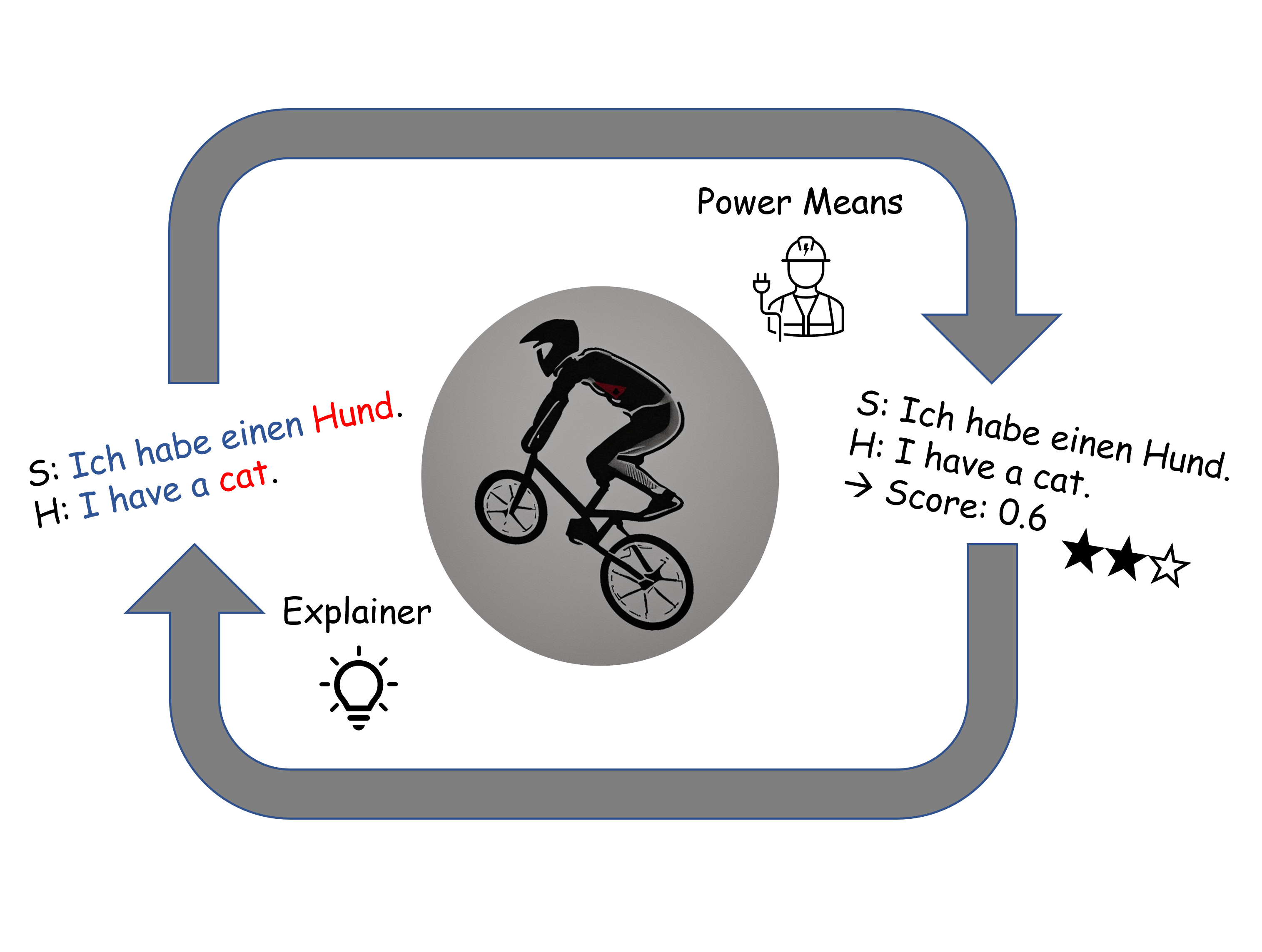
Figure 1: The duality of sentence-level machine translation evaluation metrics (right) and their word-level explanations (left).

While MTE metrics can work on different granularity levels and explanations can take on different forms, in this work, we focus on sentence-level metrics and their explainability through feature-importance techniques, where we note an intriguing duality:
Sentence-level MTE metrics return a single score indicating the translation quality of an input sentence. Feature importance explanations (e.g. Ribeiro et al., 2016) increase the granularity of this score, by assigning additional word-level scores. These scores capture additional information about the translated sentence and about the model that processed it, as explored by the Eval4NLP shared task Fomicheva et al. (2021). In recent MQM datasets, word-level error annotations are converted into sentence level scores using heuristic functions (Freitag et al., 2021a). Likewise, metrics like BERTScore Zhang et al. (2020) and BARTScore Yuan et al. (2021) build their sentence-level scores upon word-level scores. In other words, on the one hand, feature importance techniques produce word-level scores from sentence-level scores and on the other hand, heuristics can aggregate word-level scores into sentence-level scores. This duality (Belouadi and Eger, 2022) is similar to the EM algorithm Dempster et al. (1977) and we set our focus on exploring it systematically. While, due to the described relationship, we focus on MTE as a ‘natural’ use case, other regression and classification tasks follow similar settings, which makes our approach more generally applicable. Figure 1 visualizes this duality.

We propose a method that directly leverages word-level explanations to improve the original score, instead of explaining it to a human. Specifically, our method aggregates word-level feature importance explanations using power means and combines them with the original score using a linear combination. To obtain the explanations, we leverage model-agnostic explainability techniques, allowing application to any MTE metric.

We present an evaluation across five datasets where we test the improvement of five metrics using four different explainability techniques and show conditions for failure and success of the approach. Our work makes the following contributions:

• We highlight the duality of word-level explanations and sentence-level scores for MTE metrics.

• We propose an approach to improve any MTE metric by combining it with model-agnostic explainability techniques.

• We provide an evaluation that shows that our approach can reach substantial improvements for 3 of 4 datasets, when using the LIME explainer.

2 Approach

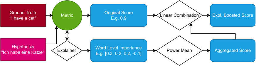
Figure 2: Boosting machine translation Metrics with Explainabilty (BMW): A metric computes an original score that we want to improve in terms of correlation to human judgments. We employ an explainer that returns word-level feature importance scores, which we aggregate into a single score using power means. Finally, we compute a new score by performing a linear combination of the aggregated and the original score.

MTE metrics grade a translated sentence, also referred to as hypothesis, by comparing it to a ground truth. The ground truth could, for example, be a human reference translation or the original source sentence. Given a pair of ground truth sentence $\boldsymbol{a}=\langle a_{1},...,a_{n}\rangle$ and hypothesis sentence $\boldsymbol{b}=\langle b_{1},...,b_{m}\rangle$, a sentence-level MTE metric $\mathcal{S}_{0}$ generates a single score $\mathcal{S}_{0}(\boldsymbol{a},\boldsymbol{b})=\textit{s}_{\textit{0}}\in\mathbb{R}$. This score can be interpreted as, for example, the similarity of $\boldsymbol{a}$ and $\boldsymbol{b}$ or the adequacy/accuracy of the translation $\boldsymbol{b}$ given $\boldsymbol{a}$.

We propose Boosting machine translation Metrics with eXplainability (BMX), a method that can work with any sentence-level MTE metric. Our algorithm consists of three steps: (1) compute feature importance explanations, (2) aggregate explanation scores, and (3) combine the aggregated explanations with the original score. Figure 2 illustrates the approach.

2.1 Feature importance computation

The input of our algorithm is an arbitrary MTE metric $\mathcal{S}_{0}$, which we aim to improve, and a pair of ground-truth and hypothesis sentences $(\boldsymbol{a},\boldsymbol{b})$. We define the explanation as a function $\mathchoice{{\scriptstyle\mathcal{E}}}{{\scriptstyle\mathcal{E}}}{{\scriptscriptstyle\mathcal{E}}}{\scalebox{0.7}{$\scriptscriptstyle\mathcal{E}$}}\in\mathcal{E}$, where $\mathcal{E}$ is a set of all feature importance explanation functions, e.g., LIME Ribeiro et al. (2016) or SHAP Lundberg and Lee (2017). $\mathchoice{{\scriptstyle\mathcal{E}}}{{\scriptstyle\mathcal{E}}}{{\scriptscriptstyle\mathcal{E}}}{\scalebox{0.7}{$\scriptscriptstyle\mathcal{E}$}}$ computes feature importance scores $\phi_{i}$ for each input feature of the model it explains (in our case a metric). As is common to many NLP setups, we consider each input token as a feature. We explain $\mathcal{S}_{0}$ and its evaluation of $\boldsymbol{a}$ and $\boldsymbol{b}$ using $\mathchoice{{\scriptstyle\mathcal{E}}}{{\scriptstyle\mathcal{E}}}{{\scriptscriptstyle\mathcal{E}}}{\scalebox{0.7}{$\scriptscriptstyle\mathcal{E}$}}$ and obtain $\phi$ with $\dim=m+n$ as follows:

$$\mathchoice{{\scriptstyle\mathcal{E}}}{{\scriptstyle\mathcal{E}}}{{\scriptscriptstyle\mathcal{E}}}{\scalebox{0.7}{$\scriptscriptstyle\mathcal{E}$}}(\mathcal{S}_{0},\boldsymbol{a},\boldsymbol{b})=\langle\phi_{1},...,\phi_{n},\phi_{n+1},...,\phi_{n+m}\rangle$$

The importance scores $\boldsymbol{\phi}$ specify the contribution of each token in $\boldsymbol{a}$ and $\boldsymbol{b}$ to $\textit{s}_{\textit{0}}$. Note that the metric $\mathcal{S}_{0}$ itself is a parameter to $\mathchoice{{\scriptstyle\mathcal{E}}}{{\scriptstyle\mathcal{E}}}{{\scriptscriptstyle\mathcal{E}}}{\scalebox{0.7}{$\scriptscriptstyle\mathcal{E}$}}$ as model-agnostic explainability functions compare the metrics’ original output with its output for permutations of the input sentences. If a metric performs reasonably well, a high feature importance $\phi_{i}$ indicates that token $t_{i}\in\boldsymbol{a}\cup\boldsymbol{b}$ has a positive contribution to the translation score $\mathcal{S}_{0}$ and thus is likely to be correctly translated. Conversely, a low feature importance indicates that a token has a small or negative contribution and thus is likely translated incorrectly. This setup follows the Eval4NLP21 Shared Task Fomicheva et al. (2021), with the difference that they consider inverted feature importance, i.e. translation errors.

2.2 Explanation score aggregation

As mentioned above, the feature importance scores of a reasonable metric indicate the translation quality of each token. We combine these values to estimate the quality of the hypothesis at the sentence level. Therefore, we employ an aggregation function $f:\mathbb{R}^{k}\rightarrow\mathbb{R}$ to transform feature importance scores generated from the previous step, into a single scalar value. We obtain the aggregated explanation score $\hat{s}_{i}$ as follows:

$$f(\mathchoice{{\scriptstyle\mathcal{E}}}{{\scriptstyle\mathcal{E}}}{{\scriptscriptstyle\mathcal{E}}}{\scalebox{0.7}{$\scriptscriptstyle\mathcal{E}$}}(\mathcal{S}_{0},\boldsymbol{a},\boldsymbol{b})))=\hat{s}_{0}$$

2.3 Linear combination

Finally, we combine $\hat{s}_{0}$ and $s_{0}$ in a linear combination using weight $w$ to construct a new metric $\mathcal{S}_{1}$:

$$\mathcal{S}_{1}(\boldsymbol{a},\boldsymbol{b})=w\cdot s_{0}+(1-w)\cdot\hat{s}_{0}=s_{1}$$

Note that $\mathcal{S}_{1}$ denotes the new metric that assigns the score to $(\boldsymbol{a},\boldsymbol{b})$ and $s_{1}$ denotes its output score for a specific instance.

We note that this three step process (feature importance computation, explanation score aggregation, linear combination) can be applied iteratively by increasing the index of $S$ (resp. $s$). E.g., in the next iteration, we can consider $S_{1}$ as the original metric and $s_{1}$ as the original score. This can be repeated as shown by Algorithm 1. This algorithm uses the same $p$, $w$, $\mathchoice{{\scriptstyle\mathcal{E}}}{{\scriptstyle\mathcal{E}}}{{\scriptscriptstyle\mathcal{E}}}{\scalebox{0.7}{$\scriptscriptstyle\mathcal{E}$}}$ and $f$ in each iteration. Note that we could also adjust these variables per iteration.

Algorithm 1 BMX Algorithm

$\mathcal{S}_{0},(\boldsymbol{a},\boldsymbol{b}),f,\mathchoice{{\scriptstyle\mathcal{E}}}{{\scriptstyle\mathcal{E}}}{{\scriptscriptstyle\mathcal{E}}}{\scalebox{0.7}{$\scriptscriptstyle\mathcal{E}$}},p,w$,

for $i\in 1,...,n$ do

     $\hat{s}_{i-1}=f(\mathchoice{{\scriptstyle\mathcal{E}}}{{\scriptstyle\mathcal{E}}}{{\scriptscriptstyle\mathcal{E}}}{\scalebox{0.7}{$\scriptscriptstyle\mathcal{E}$}}(S_{i-1},\boldsymbol{a},\boldsymbol{b})))$

     $\mathcal{S}_{i}(\boldsymbol{a},\boldsymbol{b})=w\cdot s_{i-1}+(1-w)\cdot\hat{s}_{i-1}$

end for

3 Experiment Setup

In this section, we describe the datasets, MTE metrics, explainers and aggregation methods that we evaluate in §4 and their parameter configurations.

3.1 Datasets

We evaluate our metrics by reporting their correlation with human ground truth annotations of three different datasets: the WMT17 Bojar et al. (2017) newstest2017 test set in the to-English direction, the 2020 partition of the MLQE-PE dataset Fomicheva et al. (2022) and the Eval4NLP21 testset Fomicheva et al. (2021). These contain 7 language pairs in WMT17 and MLQE-PE as well as 4 language pairs in Eval4NLP21. Each of these datasets contains source sentence - machine translation pairs and human direct assessment (DA) scores Graham et al. (2017) that grade the translation quality. To determine this translation quality, MLQE-PE and Eval4NLP21 presented the human annotators with the source and hypothesis sentence. WMT17 contains additional reference translations, which were used instead of the source by the human annotators.

Table 1 shows an overview of the number of samples per language pair and dataset. Finally, we select the testsets of the WMT22 Quality Estimation shared task Zerva et al. (2022) to test the usefulness of the approach on an unseen dataset. Some newer evaluation approaches use multidimensional quality metrics (MQM) Lommel et al. (2014); Freitag et al. (2021a) that aggregate scores from fine-grained human error annotations, instead of DA. As another unseen testset, we evaluate selected BMX configurations for the MQM annotations of newstest21 Freitag et al. (2021a).

	WMT17	Eval4NLP	MLQE-PE
LPs	cs-en	ro-en	ro-en
	de-en	et-en	et-en
	fi-en	ru-de	si-en
	lv-en	de-zh	ne-en
	ru-en		ru-en
	tr-en		en-zh
	zh-en		en-de
Per LP	560	1000	1000
Total	3920	4000	7000

Table 1: Summary of all datasets we are using for the exploration. We list the language pairs (LPs) in each set, the number of samples per pair and the total number of samples. The bold LPs occur in multiple datasets.

3.2 Base metrics

We explore the effect of our method on three reference-free metrics and two reference-based metrics as baseline metrics. We report the exact model configurations in appendix A. BLEU Papineni et al. (2002) is a widely-used reference-based metric that determines the quality of the hypothesis based on the number of matches between the n-grams of the candidate translation and a reference translation. Despite its wide usage, it has several weaknesses and does not perform well for sentence-level evaluations (e.g. Reiter, 2018; Mathur et al., 2020). Here, we use it to explore the effect of our method on a non-black-box metric. BERTScore computes a sentence score from the cosine similarity of contextualized word-embeddings between two input sentences. We use it as a reference-based metric with the Roberta-large model for English. We refer to XBERTScore as the reference-free variant of the BERTScore Zhang et al. (2020), which uses multilingual language models Zhang et al. (2020); Song et al. (2021). Leiter (2021) empirically showed that among multiple XLMR Conneau et al. (2020) model variants, one fine-tuned on a cross-lingual NLI dataset XNLI Conneau et al. (2018) achieves strong results on the Eval4NLP 2021 Fomicheva et al. (2021) dataset. Hence, we consider this variant of XLM-RoBERTa (XLM-RoBERTa NLI) for our experiments. XLMR-SBERT Reimers and Gurevych (2020) calculates multilingual sentence embeddings. We use it with XLMR to embed the ground truth and hypothesis, then compute their cosine similarity as sentence-level score. XMoverScore Zhao et al. (2020) is a reference-free adaption of MoverScore Zhao et al. (2019). The metric usually uses learned cross-lingual mappings for each languague pair and a target-side language model. Here, we omit these two steps to speed up computation and apply it to unseen language pairs (where no mapping has been trained). We include it as a weak metric to study how the effect of our method compares to better ones. Finally, as a baseline we include a mock-metric that returns a random number between 0 and 1 for any input.

3.3 Explanation techniques

We explore the effectiveness of four different model-agnostic explainers and one additional mock-explainer as a baseline.

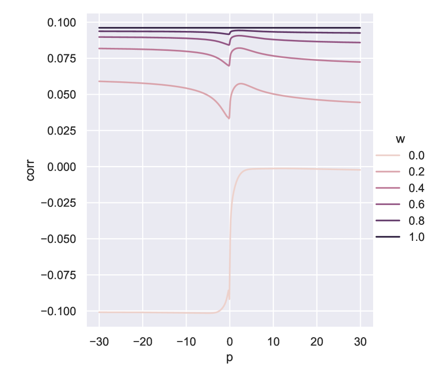
(a) Erasure + XMoverScore, en-zh from MLQE-PE

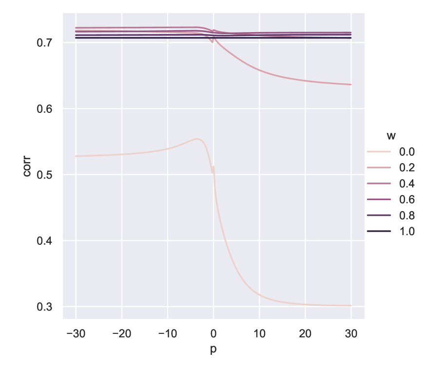
(b) LIME + BERTScore, et-en from Eval4NLP

Figure 3: Two plots of Pearson correlations on a selected dataset, explainer and metric, with varying $p$ and $w$ values. $w=1$ is the original metric. In the left plot, our approach doesn’t show any improvements. However, in the right plot, there are improvements over $w=1$.

Erasure: Li et al. (2016) suggest neural network decisions can be investigated by analyzing the effect of feature removal. We use Erasure to determine token-level importance scores by analyzing a metric’s prediction with respect to the presence of each token in the translation. This is for example also done in adversarial attacks by Li et al. (2020). For each token $t_{i}\in\boldsymbol{a}\cup\boldsymbol{b}$ we compute the importance $\phi_{i}$ as follows:

$$\phi_{i}=\mathcal{S}(\boldsymbol{a},\boldsymbol{b})-\mathcal{S}(\boldsymbol{a},\boldsymbol{b})_{/t_{i}}$$

where $\mathcal{S}(\boldsymbol{a},\boldsymbol{b})$ is a MTE metric grading the ground truth $\boldsymbol{a}$ and hypothesis $\boldsymbol{b}$. $\mathcal{S}(\boldsymbol{a},\boldsymbol{b})_{/t_{i}}$ denotes the same input without token $t_{i}$.

LIME Ribeiro et al. (2016): When we explain a metric with LIME, for each ground truth or hypothesis sentence that is explained, LIME trains a linear model that returns similar results as the metric in a neighborhood of this sentence. The dataset used to fit this model is generated by randomly permuting the input. The labels of this dataset are determined by computing the metric score of these permuted sentences. Finally, the weights of the linear model are assigned to each token as feature importance explanations. We run LIME with 100 permutations per ground truth and per reference sentence.

SHAP Lundberg and Lee (2017) is an explainability technique that either exactly or approximately computes Shapley values from game theory and assigns these as feature importances. The exact SHAP explanation of a token is calculated using all possible permutations of the target sentence (with a single replacement token). As a result, feature importance is not the difference between $\mathcal{S}(\boldsymbol{a},\boldsymbol{b})$ with or without a token, rather it is a contribution of a token to the difference between the score of original and the mean score of all permutations. The number of possible permutations grows exponentially with the number of input features (here tokens). For this reason, SHAP is often approximated, e.g. using KernelShap Lundberg and Lee (2017). In our experiments, we use the same replacement string as for LIME: UNKWORDZ. Also, up to a number of 7 tokens per sentence, we compute the exact SHAP. For longer sentences, we use PermutationSHAP, which is the default option of the SHAP library.

Input Marginalization: Kim et al. (2020) suggest that replacement with empty strings or unreasonable tokens causes out-of-distribution problems in the explained model, which might lead to a decrease in accuracy of the explanation. Instead, their technique uses a masked-language model to generate a list of the most reasonable replacement tokens and investigates the effect that replacement with each of them has in comparison to the original score. We adapt their technique for metrics and choose to only consider replacement tokens with a probability of more than 5% to keep the computation efficient. We give more details on this explainer in appendix D. In our figures, we abbreviate this explainer as IM.

Random Explainer: This mock explainer returns a random number between 0 and 1 for each input token: $\phi_{i}=random(0,1)$.

3.4 Aggregation technique

Following Rücklé et al. (2018), we use the power mean (also known as generalized mean) as a generalization over different means to aggregate token-level attribution scores. The power mean of $n$ positive numbers $e_{1},\ldots,e_{n}$ is computed as:

$$M_{p}(e_{1},...,e_{n})=\left(\frac{1}{n}\sum_{k=1}^{n}e^{p}_{k}\right)^{\frac{1}{p}}$$

Depending on $p$, the power mean takes on the value of specific means, e.g.  $p=-1$ is the harmonic mean, $p=1$ is the arithmetic mean, and $p=-\infty$ resp. $p=+\infty$ is the minimum resp. maximum. We experiment with different $p$-values between $[-30,30]$ in $0.1$ steps. The token-level scores resulting from the explanation technique can be negative, which is problematic for power means, as these are defined on positive numbers only. To guarantee positive importance scores, whenever there is a negative importance score for a token, we add a regularization term to all importance scores of the current ground-truth/hypothesis pair. This term is the absolute value of the smallest importance score assigned to any token of this pair. Generally, we add a constant $1\mathrm{e}{-9}$ to each importance score to avoid issues with fluctuations around 0.

4 Results and analysis

In this section, we evaluate the effectiveness of our evaluation metric by correlating the results with human judgments of translation quality annotated in the datasets described in §3.1. We describe the Pearson correlations that we compute as follows:

$$\text{Pearson}(\>H(\textit{LP},D)\>,\>S_{1}(\textit{LP},D,S_{0},\mathchoice{{\scriptstyle\mathcal{E}}}{{\scriptstyle\mathcal{E}}}{{\scriptscriptstyle\mathcal{E}}}{\scalebox{0.7}{$\scriptscriptstyle\mathcal{E}$}},w,p)\>)$$

Here, $H$ returns the set of human scores for language pair LP and dataset $D$. $S_{1}$ returns the new metric scores, when our method is applied to LP and $D$. Its further parameters are the original metric $S_{0}$, the explainer $\mathchoice{{\scriptstyle\mathcal{E}}}{{\scriptstyle\mathcal{E}}}{{\scriptscriptstyle\mathcal{E}}}{\scalebox{0.7}{$\scriptscriptstyle\mathcal{E}$}}$, the weight of the linear combination $w$ and the $p$-value of the power mean. We apply this Pearson correlation across all experiment settings introduced in §3 and compute $1,290,000$ correlation scores (see Appendix B for details). Figure 3 shows two examples of how the correlation behaves for different $p$ and $w$ values in a setting with fixed LP, $D$, $S_{0}$ and $\mathchoice{{\scriptstyle\mathcal{E}}}{{\scriptstyle\mathcal{E}}}{{\scriptscriptstyle\mathcal{E}}}{\scalebox{0.7}{$\scriptscriptstyle\mathcal{E}$}}$. The first example shows a case where no improvement over the original metric ($w=1$) is reached for any $p$ and $w$. The second example shows a case with good improvement for (among others) $w=0.4$. Generally, there are cases for which our new metric $S_{1}$ improves over $S_{0}$ and cases in which it does not. This motivates the remainder of this section, where we use the correlation scores to assess the overall performance, determine the best parameters and analyze in which cases the approach performs best. Finally, we explore the performance for a fixed set of parameters on two held out datasets. In appendix E, we discuss the results of performing a second iteration, which did not considerably improve on the first.

4.1 Performance across all parameters

Figure 4 shows kernel density estimations of the difference between the correlation of the original metric (for $w=1$) and correlations for the new metric(s) (for $w\in\{0,0.2,0.4,0.6,0.8\}$ across all other parameters). The results are plotted separately for every explainer. We can see that the density across all explainers is skewed to the left. I.e., generally, our approach decreases the original metric’s performance. However, there are also datapoints to the right of the zero value of the x-axis (marked by a black line), leading to the question whether we can select parameters that lead to an improvement in most cases. We also evaluate the success cases per explainer and find that the random explainer indeed has the least cases of improvement, so we exclude it and the random metric for further experiments, in order to not have them reflected in the results. The reason we described them up to this point is that comparison with them allowed us to verify that our approach is better than a random baseline.

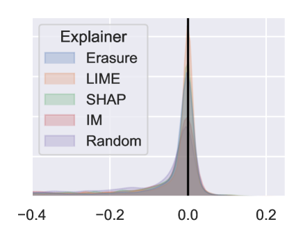
Figure 4: Difference in Pearson correlation to human judgements between the new metric and the original metric across all experiment settings

4.2 Finding the best parameters

We consider which values of the parameters $w$ and $p$ lead to the highest improvements. To do so, for every combination of the language pair LP, dataset $D$, metric $S_{0}$, and explainer $\mathchoice{{\scriptstyle\mathcal{E}}}{{\scriptstyle\mathcal{E}}}{{\scriptscriptstyle\mathcal{E}}}{\scalebox{0.7}{$\scriptscriptstyle\mathcal{E}$}}$ we filter for the $p$ and $w$ values that increase the correlation between the scores returned by our approach and the human scores in the datasets the most. Further, we exclude the results of the random explainer and random metric. By doing so, we consider the best $p$ and $w$ values for $272$ experiment settings. Figure 5 shows the box-plots of the $p$ and $w$ in these $272$ settings. For further experiments, we choose the median $p$ and $w$ values for each explainer, as shown in the box-plots, e.g., $w=0.4$ and $p=-1.4$ for LIME. Interestingly, LIME has the lowest Median for $w$, i.e., the linear combination puts more weight on the explanations compared to the other explainers. This is already an indicator that LIME performs best among them. We also note that its $p$-median is close to $-1$, which is the harmonic mean. Future work could explore other ways to select these two parameters, e.g., instead of filtering for those $p$ and $w$ that led to the highest increase in terms of correlation to human judgments, filtering for those that increase the correlation across most experiment settings.

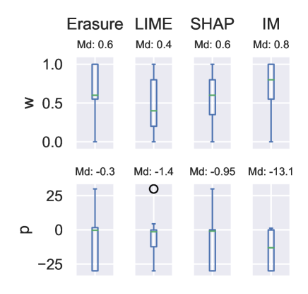
Figure 5: Box-plots of the $w$ and $p$ values leading to the highest correlation improvements across all experiment settings (excluding the Random Explainer and Metric). Md denotes the Median value.

4.3 Analysis with fixed $p$ and $w$

Figure 6 compares the number of improvements vs. decreases of correlation with fixed $w$ and $p$ across every combination of language pair LP, dataset $D$, original metric $S_{0}$ and explainer $\mathchoice{{\scriptstyle\mathcal{E}}}{{\scriptstyle\mathcal{E}}}{{\scriptscriptstyle\mathcal{E}}}{\scalebox{0.7}{$\scriptscriptstyle\mathcal{E}$}}$ across $\mathchoice{{\scriptstyle\mathcal{E}}}{{\scriptstyle\mathcal{E}}}{{\scriptscriptstyle\mathcal{E}}}{\scalebox{0.7}{$\scriptscriptstyle\mathcal{E}$}}$ (excluding the random explainer and metric). We can see that LIME and SHAP show more cases of improvement. This suggests that fixing $p$ and $w$, as described in §4.2, makes our method perform well in a reasonable amount of cases. To further distinguish the experiment settings that work well from those that do not, we perform a linear ridge regression between LP, $D$, $S_{0}$ and $\mathchoice{{\scriptstyle\mathcal{E}}}{{\scriptstyle\mathcal{E}}}{{\scriptscriptstyle\mathcal{E}}}{\scalebox{0.7}{$\scriptscriptstyle\mathcal{E}$}}$. Figure 8 shows the three biggest and the three smallest learned coefficients. Based on these coefficients, the language pairs en-zh and si-en seem to be difficult to improve with our approach, while tr-en and de-zh are indicators for larger expected improvement. Further, the reference-based BERTScore variant seems to be especially hard to improve. Lastly, our technique is likely to work on the MLQE-PE corpus. We note that the regressors are not completely independent. Still, this evaluation gives an impression of good and bad conditions for the approach.

LIME

The results shown up to now investigate the performance across all combinations of language pair LP, dataset $D$ and original metric $S_{0}$ separately for each explainer $\mathchoice{{\scriptstyle\mathcal{E}}}{{\scriptstyle\mathcal{E}}}{{\scriptscriptstyle\mathcal{E}}}{\scalebox{0.7}{$\scriptscriptstyle\mathcal{E}$}}$. For the next experiments, we solely select the explainer that performed best: LIME. Figure 7 plots the distribution of correlations across every combination of language pair LP and original metric $S_{0}$ separated for each dataset $D$. We can see that the distributions for Eval4NLP and MLQE-PE are skewed to the right, while it is skewed to the left for WMT17, suggesting that some datasets are harder to improve on than others. Specifically, the human scores in WMT17 are based on reference sentences instead of the source, while most tested metrics are reference-free which might be a reason for this. In Appendix C, we analyze the effects of LP and $S_{0}$ in more detail.

In our experiments on the effect of the original metric $S_{0}$, we find that reference-based BERTScore and SentenceBLEU do not improve in most cases. SentenceBleu is especially stable, as it also does not perform a lot worse across experiments. This might because SentenceBleu is a hard metric. The metrics that improved the most were reference-free XBertScore and XLMR-SBERT.

Performance improvements

We also check the correlation between the original metric’s correlation and its change with out method:

$$\text{Pearson(}C_{1}-C_{0},C_{0})$$

Here, $C_{1}$ is the mean correlation of the BMX metrics across all datasets and $C_{0}$ is the mean correlation of the original metrics across all datasets. This correlation is negative ($-0.286$), which shows that metrics that originally performed worse tend to be easier to improve. Based on these results, we advise to use our enhancement in cases where the data is suspected to be difficult for a metric. Further, we propose to use the mean $w$ and $p$ found in §4.2 for the tested explainers. Among the tested explainers, LIME performed best and reference-free metrics seemed to improve more (though reference-based metrics were only tested on one dataset).

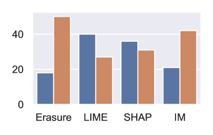
Figure 6: Cases of improvement and decreased performance with $p$ and $w$ fixed to the respective explainer’s best median. The blue bars show the number of settings with improved correlation, the orange bars show the number of settings with equal or worse correlation.

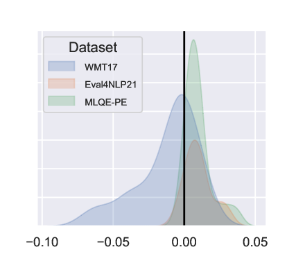
Figure 7: Density plot of correlation improvements with LIME across datasets. The x-axis shows the correlation difference between the new and original metric.

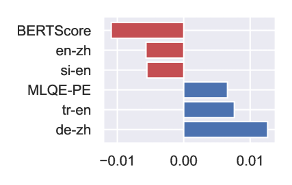
Figure 8: Three most and three least important regressors using ridge regression with $p$ and $w$ fixed to the median of the highest correlation improvements fitted across all other datapoints.

4.4 Performance on WMT22

We apply the gathered settings to the test sets of WMT22 (which we held back in the previous evaluation) and plot the number of times the correlation did improve across reference-free metrics in Figure 9. We can see that the method indeed increased the correlation in more cases than it decreased it. Also, we see that each original metric has a relatively low average correlation of $0.1$ to $0.29$. Figure 10 highlights the number of cases where our technique provides an improvement. Especially the enhancement using LIME works in $15$ out of $18$ settings and is stronger than on the previously analyzed datasets. The maximal improvement achieved with the fixed hyperparameters in these $18$ settings is $0.032$

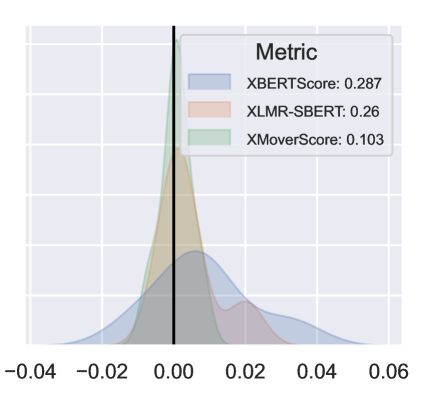
Figure 9: Density plot of correlation improvements with LIME across different metrics on WMT22. The x-axis shows the correlation difference between the new and original metric.

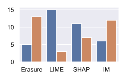
Figure 10: Comparison of explainers using the $p$ and $w$ values from the analysis in §4.3 on WMT22. The blue bars show the number of settings with improved correlation, the orange bars show the number of settings with equal or worse correlation.

4.5 Performance for an MQM dataset

We evaluate the performance of LIME with XBERTScore and XLMR-SBERT on another held back dataset, the MQM newstest21 annotations Freitag et al. (2021a). The original correlation is low and we find that the preselected $p$ and $w$ improve over the base metric in all 4 settings. Figure 11 shows the behavior for different $p$ and $w$ values. We can also see that the setting we preselect for LIME, $w=0.4$ and $p=-1.4$, leads to better results than the original metric in both plots, but choices of lower $w$ would be have performed even better. We find that the maximal correlation gain for these settings of $w$ and $p$ for the 4 experiment settings is $0.055$.

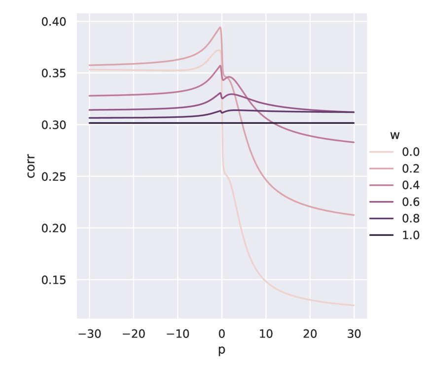
(a) Pearson correlation for zh-en, with LIME and XBERTScore.

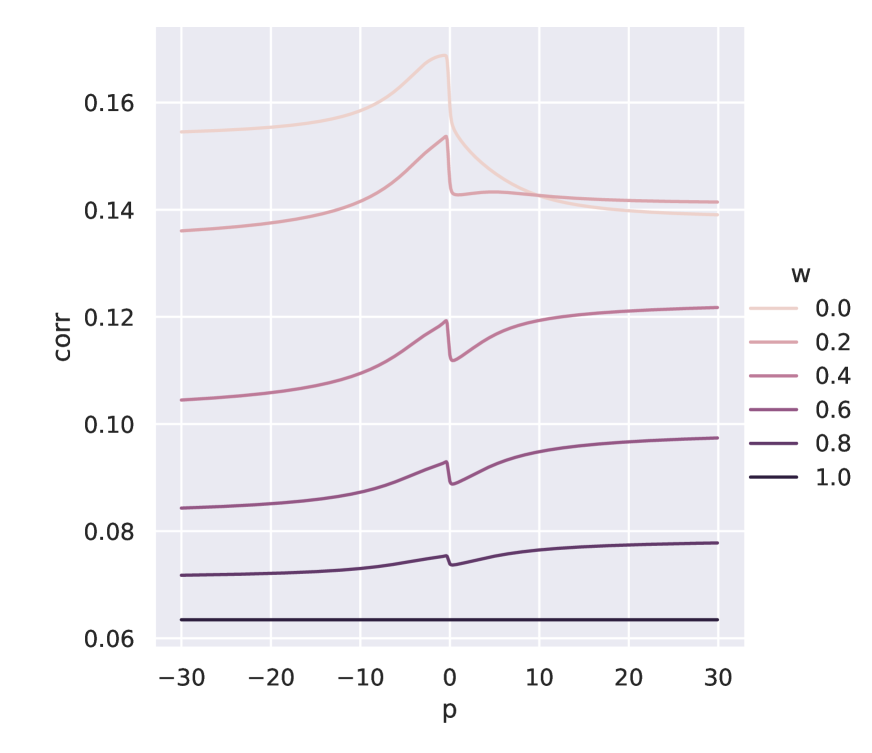
(b) Pearson correlation for en-de, with LIME and XBERTScore.

Figure 11: Experiment results for Newstest21 MQM annotations, across $p$ values from $-30$ to $30$ and across $w$ values from $0$ to $1$, where $w=1$ is the original metric (indicated by a black line).

5 Related Work

By combining methods from the explainability domain and MTE metrics, our work is related to both fields.

MTE Metrics

Hard reference-based metrics like BLEU Papineni et al. (2002) and ChrF Popović (2015) grade translations based on character- or word-level overlap with a reference sentence and often fall short when synonyms or paraphrasations of this reference are used in a translation. Modern soft reference-based metrics like BERTScore Zhang et al. (2020) and BLEURT Sellam et al. (2020) instead leverage contextualized word-embeddings and neural network architectures to allow for a soft matching of the reference and the hypothesis sentence. However, these metrics still require a reference translation that in some cases has to be provided by a human expert. Reference-free metrics like XBERTScore (e.g. Zhang et al., 2020; Song et al., 2021; Leiter, 2021) or XMoverScore Zhao et al. (2020) do not require this precondition by directly computing similarity with the source sentence instead of an additional reference. For a further overview of MTE metrics, we refer to Celikyilmaz et al. (2020); Sai et al. (2022).

Explainable MTE metrics

While soft metrics perform better than hard metrics, their internal workings have become more complex and can not be easily understood by a human anymore. The recent shared tasks Eval4NLP (Fomicheva et al., 2021) and WMT22 QE (Zerva et al., 2022) explore the usage of explainability techniques to tackle this issue and provide word-level explanations for sentence-level metrics. Motivated by their work, our work also uses word-level explanations, but additionally aggregates them in order to improve the original score.

Considering existing metrics, our work is especially related to word-level metrics and metrics that can be considered self-explaining. Word-level metrics like word-level Transquest Ranasinghe et al. (2021) and Ding et al. (2021) are designed to directly assign translation quality scores to each word instead of the whole sentence. As such, they can be considered as self-explaining, as they provide the same kind of explanations external explainers would provide for a sentence level model Leiter et al. (2022). We note that word-level scores might also be limited in the quality of explanation they provide, though this is not a focus of this paper and we leave the exploration of further methods to future work. Some existing sentence-level metrics are self-explaining in this sense as well, as they use sentence-level scores that are constructed from other word-level outputs. E.g. BERTScore is based on word-level cosine similarities of contextualized word-embeddings and BARTScore Yuan et al. (2021) is based on word-level prediction probabilities of an MBART translation model. Our method relates to word-level and self-explaining methods, because we also use word-level scores in order to construct a new sentence level score. However, to the best of our knowledge, our method is the first to leverage model-agnostic explainabiltiy techniques to extract additional word-level information that is incorporated into the final metric. This has the benefit of being applicable to any kind of MTE metric (and theoretically to any kind of NLG metric).

Another topic related to explainable MTE metrics are fine-grained annotation schemes themselves. For example, the word-level scores annotated in the Eval4NLP shared task Fomicheva et al. (2021) or fine-grained error annotations like MQM Lommel et al. (2014) allow for human annotation of explanations that could for example be used to compare the word-level scores in our experiments to.

Explainability

Our method is related to the field of explainability, as we leverage model-agnostic explainability techniques to collect word-level importance scores. There are many concept papers and surveys that give an overview of this area, e.g. Lipton (2018); Doshi-Velez and Kim (2017); Barredo Arrieta et al. (2020).

Specifically, we want to highlight the similarity of our approach to the concept of simulatability (e.g. Hase and Bansal, 2020). To test how well an explanation technique performs, some works conduct simulatability tests. In these, a machine or a human tester tries to reproduce an original model’s output or solve an additional task, using the explanations they receive about it. Our work relates to this topic, as we also utilize explanation outputs to accomplish a specific task. However, our focus is not on evaluating the performance of the explainers, but rather on using them to improve metrics for MTE.

EM algorithm

Our approach for estimating the sentence-level score using an iterative method is inspired by the Expectation Maximization Algorithm (EM-algorithm) Dempster et al. (1977), which involves an iterative process to find maximum likelihood or MAP estimates of parameters. The EM algorithm aims to use the available observed data to estimate missing data and then uses that data to update the values of the parameters in the maximization step. In our case, the available data is the initial sentence score estimated with automatic MT evaluation metrics. The expectation step approximates the token-level scores from the sentence score. In the maximization step, we use the token scores to update the sentence score.

6 Conclusion

In this work, we have presented BMX: Boosting machine translation Metrics with eXplainability, a novel approach that leverages the duality of MTE metrics and feature importance explanations to boost the metrics performance. As BMX leverages model-agnostic explainability techniques, it can be applied to any machine translation evaluation metric. Additionally, it requires no supervision once the initial parameters for $p$ and $w$ are set, which might benefit fully unsupervised approaches like UScore Belouadi and Eger (2022) as well. Our tests have shown strong improvements for 4 out of 5 datasets. Notably, BMX with the LIME explainer and preselected parameters, i.e. $p=-1.4$ and $w=0.4$, achieves improvement in $\frac{15}{18}$ experiment settings of WMT22 and in all four tested conditions of the newstest21 mqm dataset. To the best of our knowledge, our approach is the first to leverage the duality of sentence-level MTE metrics and their explanations directly and we believe that it can lead a step forward in research towards true human level machine translation evaluation.

7 Limitations

One limitation of our work is that we were only able to run a few experiments for the second iteration due to efficiency constraints. Future work might consider using model distillation by training a distilled metric from the boosted setup after every iteration for speedup.

In §5, we discuss metrics that produce word-level scores or are self-explaining by default. While not applicable to all metrics, every metric that falls into one of these two groups has another option to compute explanations. As the Eval4NLP shared task showed, these tend do be stronger than model agnostic approaches Fomicheva et al. (2021). Also, while not explicitly denoted as explanations, they are often already incorporated into the final score, e.g. for BERTScore or BARTScore. Here, we note that our method can provide another way of incorporating these word-level scores into the final prediction that might be explored by future work. Future work might also explore to use other model-specific explainers, e.g.  gradient based or attention based methods (e.g. Treviso et al., 2021).

Appendix A Library Configurations

We use the following library and metric versions:

• LIME: 0.2.0.1

• SHAP: 0.41.0

• transformers: 4.20.1, 4.24.0

• BERTScore, Reference-Based: bertscore: 0.3.11; roberta-large

• XBERTScore, Reference-Free: bertscore: 0.3.11; joeddav/xlm-roberta-large-xnli

• SentenceBleu: 2.2.0

• XLMR-SBERT: stsb-xlm-r-multilingual

• XMoverScore: V2 - June 2022

The other two explainers use an own implementation.

Appendix B Number of correlation scores

We conducted our experiments with the settings introduced in section 3. This results in $6\text{metrics}\cdot 5\text{explainers}\cdot 7\text{Language Pairs}=210$ for WMT17 and $4\text{metrics}\cdot 5\text{explainers}\cdot(4+7)\text{Language Pairs}=220$ for the other two datasets. I.e. we conducted $430$ experiment settings. In each setting, we evaluated $5$ values of $w$ and $600$ values of $p$. Each of these combinations resulted in new metric scores for a specific language pair in a specific dataset. We evaluated the quality of these new scores with their specific sets using pearson correlation, resulting in $1.290.000$ correlation scores.

Appendix C Impact of language pairs and metrics, when using the three main datasets

To investigate the effect of different language pairs we select ru-en and ro-en, which each occur in two datasets, and cs-en, si-en, ru-de and plot them in figure 12. We can see that three of the LP’s correlation improvements are more centered at 0, while cs-en and ru-en have a higher variance. Improvement can be seen in all of the language pairs, though ro-en improved the most. While the language pairs are correlated with the datasets they stem from, this might also indicate that the performance of our approach also depends on the language pair.

Figure 13 shows density plots across different original metrics. we can see that BERTScore (which only ran on WMT17) has the best average performance, while XMoverScore has the worst average performance. We can also see, that BERTScore and SentenceBleu did only improve in a very small amount of cases, while the other 3 metrics improved more substantially.

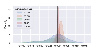
Figure 12: Density plot of correlation improvements with LIME across selected language pairs.

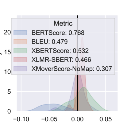
Figure 13: Density plot of correlation improvements with LIME across original metrics. The numbers denote the average original correlation.

Appendix D Input Marginalization Explainer

Here, we explain the input marginalization explainer. We denote V as the set of replacement tokens with a probability $p(t^{*}_{i}|\text{mask}_{t_{i}})>\delta$, where $\text{mask}_{t_{i}}$ denotes the input strings with token $t_{i}$ being masked, $t^{*}_{i}$ is an arbitrary token of the model vocabulary replacing $t_{i}$ and $\delta$ is the threshold of how many replacements should be considered. We first determine the effect of the replacements and then calculate the importance $\phi_{i}$ by subtracting the effect from the original score:

$$\text{effect}_{t_{i}}=\sum_{t^{\prime}_{i}\in V}S_{0}(\text{input}_{t^{\prime}_{i}})\cdot p(t^{\prime}_{i}|\text{mask}_{t_{i}})$$

$$\phi_{i}=S_{0}(\text{input})-\text{effect}_{t_{i}}$$

Here, $\text{input}_{t^{\prime}_{i}}$ refers to the input (ground truth and hypothesis), where token $t_{i}$ has been replaced with $t^{\prime}_{i}$ from the set of replacement candidates.

Appendix E Further Iterations

Our experiments show substantial improvement in just a single iteration. As described in §2, we also consider whether multiple iterations continue to improve the baseline metric. A limitation of running multiple iterations is that the number of necessary inference steps grows exponentially. This is caused by the explainers that need to perform inference on multiple permutations. As the explainers in further iterations depend on the results of the explainers in the first iterations, the approach becomes inefficient quite fast. Thus, we limit our test of further iterations to a subset of experiment settings.

In particular, we employ the combination of XBERTScore/XLMR-SBERT as the base metric and Erasure as the explainer on Eval4NLP. Erasure is the fastest of the explainers, as it only performs one permutation and inference with the original metric per input token. It is worth highlighting the value of $p$ and $w$ can be configured differently for each iteration. To keep the computation efficient, we reuse the optimal $p$ and $w$ values that we describe in §5 for the first iteration. These settings amount to an evaluation of 8 language pairs. Unfortunately, we can not see any major improvement over the first iteration for any language pair. Interestingly, scores are even very similar to the first iteration for every $p$ and $w$ (comparing free $p$ and $w$ in the first iteration with fixed $p$ and $w$ in the first and free in the second iteration). On further consideration, this is not surprising, as we chose $p=-0.3$ and $w=0.6$ for the first iteration. Hence, the score of the first iteration is close to the original score. Further, we still have a 60% part of the original metric and 40% of the aggregated explanations that is suspected to be similar as well (as it explains the original). Following this, we hypothesize that the improvement of further iterations might often be low.

References

- Barredo Arrieta et al. (2020) Alejandro Barredo Arrieta, Natalia Díaz-Rodríguez, Javier Del Ser, Adrien Bennetot, Siham Tabik, Alberto Barbado, Salvador Garcia, Sergio Gil-Lopez, Daniel Molina, Richard Benjamins, Raja Chatila, and Francisco Herrera. 2020. Explainable artificial intelligence (xai): Concepts, taxonomies, opportunities and challenges toward responsible ai. Information Fusion, 58:82–115.
- Belouadi and Eger (2022) Jonas Belouadi and Steffen Eger. 2022. Uscore: An effective approach to fully unsupervised evaluation metrics for machine translation. ArXiv, abs/2202.10062.
- Bojar et al. (2017) Ondřej Bojar, Yvette Graham, and Amir Kamran. 2017. Results of the WMT17 metrics shared task. In Proceedings of the Second Conference on Machine Translation, pages 489–513, Copenhagen, Denmark. Association for Computational Linguistics.
- Celikyilmaz et al. (2020) Asli Celikyilmaz, Elizabeth Clark, and Jianfeng Gao. 2020. Evaluation of text generation: A survey. ArXiv, abs/2006.14799.
- Conneau et al. (2020) Alexis Conneau, Kartikay Khandelwal, Naman Goyal, Vishrav Chaudhary, Guillaume Wenzek, Francisco Guzmán, Edouard Grave, Myle Ott, Luke Zettlemoyer, and Veselin Stoyanov. 2020. Unsupervised cross-lingual representation learning at scale. In Proceedings of the 58th Annual Meeting of the Association for Computational Linguistics, pages 8440–8451, Online. Association for Computational Linguistics.
- Conneau et al. (2018) Alexis Conneau, Ruty Rinott, Guillaume Lample, Adina Williams, Samuel Bowman, Holger Schwenk, and Veselin Stoyanov. 2018. XNLI: Evaluating cross-lingual sentence representations. In Proceedings of the 2018 Conference on Empirical Methods in Natural Language Processing, pages 2475–2485, Brussels, Belgium. Association for Computational Linguistics.
- Dempster et al. (1977) Arthur P. Dempster, Nan M. Laird, and Donald B. Rubin. 1977. Maximum likelihood from incomplete data via the em - algorithm plus discussions on the paper.
- Ding et al. (2021) Shuoyang Ding, Marcin Junczys-Dowmunt, Matt Post, Christian Federmann, and Philipp Koehn. 2021. The JHU-Microsoft submission for WMT21 quality estimation shared task. In Proceedings of the Sixth Conference on Machine Translation, pages 904–910, Online. Association for Computational Linguistics.
- Doshi-Velez and Kim (2017) Finale Doshi-Velez and Been Kim. 2017. Towards a rigorous science of interpretable machine learning. arXiv: Machine Learning.
- Fomicheva et al. (2021) Marina Fomicheva, Piyawat Lertvittayakumjorn, Wei Zhao, Steffen Eger, and Yang Gao. 2021. The Eval4NLP shared task on explainable quality estimation: Overview and results. In Proceedings of the 2nd Workshop on Evaluation and Comparison of NLP Systems, pages 165–178, Punta Cana, Dominican Republic. Association for Computational Linguistics.
- Fomicheva et al. (2022) Marina Fomicheva, Shuo Sun, Erick Fonseca, Chrysoula Zerva, Frédéric Blain, Vishrav Chaudhary, Francisco Guzmán, Nina Lopatina, Lucia Specia, and André F. T. Martins. 2022. MLQE-PE: A multilingual quality estimation and post-editing dataset. In Proceedings of the Thirteenth Language Resources and Evaluation Conference, pages 4963–4974, Marseille, France. European Language Resources Association.
- Fort and Couillault (2016) Karën Fort and Alain Couillault. 2016. Yes, we care! results of the ethics and natural language processing surveys. In Proceedings of the Tenth International Conference on Language Resources and Evaluation (LREC 2016), pages 1593–1600, Portorož, Slovenia. European Language Resources Association (ELRA).
- Freitag et al. (2021a) Markus Freitag, George Foster, David Grangier, Viresh Ratnakar, Qijun Tan, and Wolfgang Macherey. 2021a. Experts, errors, and context: A large-scale study of human evaluation for machine translation. Transactions of the Association for Computational Linguistics, 9:1460–1474.
- Freitag et al. (2021b) Markus Freitag, Ricardo Rei, Nitika Mathur, Chi-kiu Lo, Craig Stewart, George Foster, Alon Lavie, and Ondřej Bojar. 2021b. Results of the WMT21 metrics shared task: Evaluating metrics with expert-based human evaluations on TED and news domain. In Proceedings of the Sixth Conference on Machine Translation, pages 733–774, Online. Association for Computational Linguistics.
- Graham et al. (2017) Yvette Graham, Timothy Baldwin, Alistair Moffat, and Justin Zobel. 2017. Can machine translation systems be evaluated by the crowd alone. Natural Language Engineering, 23(1):3–30.
- Hase and Bansal (2020) Peter Hase and Mohit Bansal. 2020. Evaluating explainable AI: Which algorithmic explanations help users predict model behavior? In Proceedings of the 58th Annual Meeting of the Association for Computational Linguistics, pages 5540–5552, Online. Association for Computational Linguistics.
- Kim et al. (2020) Siwon Kim, Jihun Yi, Eunji Kim, and Sungroh Yoon. 2020. Interpretation of NLP models through input marginalization. In Proceedings of the 2020 Conference on Empirical Methods in Natural Language Processing (EMNLP), pages 3154–3167, Online. Association for Computational Linguistics.
- Leiter et al. (2022) Christoph Leiter, Piyawat Lertvittayakumjorn, M. Fomicheva, Wei Zhao, Yang Gao, and Steffen Eger. 2022. Towards explainable evaluation metrics for natural language generation. ArXiv, abs/2203.11131.
- Leiter (2021) Christoph Wolfgang Leiter. 2021. Reference-free word- and sentence-level translation evaluation with token-matching metrics. In Proceedings of the 2nd Workshop on Evaluation and Comparison of NLP Systems, pages 157–164, Punta Cana, Dominican Republic. Association for Computational Linguistics.
- Li et al. (2016) Jiwei Li, Will Monroe, and Dan Jurafsky. 2016. Understanding neural networks through representation erasure. ArXiv, abs/1612.08220.
- Li et al. (2020) Linyang Li, Ruotian Ma, Qipeng Guo, Xiangyang Xue, and Xipeng Qiu. 2020. BERT-ATTACK: Adversarial attack against BERT using BERT. In Proceedings of the 2020 Conference on Empirical Methods in Natural Language Processing (EMNLP), pages 6193–6202, Online. Association for Computational Linguistics.
- Lipton (2018) Zachary C. Lipton. 2018. The mythos of model interpretability. Commun. ACM, 61(10):36–43.
- Lommel et al. (2014) Arle Lommel, Aljoscha Burchardt, and Hans Uszkoreit. 2014. Multidimensional quality metrics (mqm): A framework for declaring and describing translation quality metrics. Tradumàtica: tecnologies de la traducció, 0:455–463.
- Lundberg and Lee (2017) Scott M Lundberg and Su-In Lee. 2017. A unified approach to interpreting model predictions. In Advances in Neural Information Processing Systems, volume 30. Curran Associates, Inc.
- Mathur et al. (2020) Nitika Mathur, Timothy Baldwin, and Trevor Cohn. 2020. Tangled up in BLEU: Reevaluating the evaluation of automatic machine translation evaluation metrics. In Proceedings of the 58th Annual Meeting of the Association for Computational Linguistics, pages 4984–4997, Online. Association for Computational Linguistics.
- Papineni et al. (2002) Kishore Papineni, Salim Roukos, Todd Ward, and Wei-Jing Zhu. 2002. Bleu: a method for automatic evaluation of machine translation. In Proceedings of the 40th Annual Meeting of the Association for Computational Linguistics, pages 311–318, Philadelphia, Pennsylvania, USA. Association for Computational Linguistics.
- Popović (2015) Maja Popović. 2015. chrF: character n-gram f-score for automatic MT evaluation. In Proceedings of the Tenth Workshop on Statistical Machine Translation, pages 392–395, Lisbon, Portugal. Association for Computational Linguistics.
- Ranasinghe et al. (2021) Tharindu Ranasinghe, Constantin Orasan, and Ruslan Mitkov. 2021. An exploratory analysis of multilingual word-level quality estimation with cross-lingual transformers. In Proceedings of the 59th Annual Meeting of the Association for Computational Linguistics and the 11th International Joint Conference on Natural Language Processing (Volume 2: Short Papers), pages 434–440, Online. Association for Computational Linguistics.
- Reimers and Gurevych (2020) Nils Reimers and Iryna Gurevych. 2020. Making monolingual sentence embeddings multilingual using knowledge distillation. In Proceedings of the 2020 Conference on Empirical Methods in Natural Language Processing (EMNLP), pages 4512–4525, Online. Association for Computational Linguistics.
- Reiter (2018) Ehud Reiter. 2018. A structured review of the validity of BLEU. Computational Linguistics, 44(3):393–401.
- Ribeiro et al. (2016) Marco Tulio Ribeiro, Sameer Singh, and Carlos Guestrin. 2016. ”why should I trust you?”: Explaining the predictions of any classifier. In Proceedings of the 22nd ACM SIGKDD International Conference on Knowledge Discovery and Data Mining, San Francisco, CA, USA, August 13-17, 2016, pages 1135–1144.
- Rücklé et al. (2018) Andreas Rücklé, Steffen Eger, Maxime Peyrard, and Iryna Gurevych. 2018. Concatenated p-mean word embeddings as universal cross-lingual sentence representations. ArXiv, abs/1803.01400.
- Sai et al. (2022) Ananya B. Sai, Akash Kumar Mohankumar, and Mitesh M. Khapra. 2022. A survey of evaluation metrics used for nlg systems. ACM Comput. Surv., 55(2).
- Sellam et al. (2020) Thibault Sellam, Dipanjan Das, and Ankur Parikh. 2020. BLEURT: Learning robust metrics for text generation. In Proceedings of the 58th Annual Meeting of the Association for Computational Linguistics, pages 7881–7892, Online. Association for Computational Linguistics.
- Song et al. (2021) Yurun Song, Junchen Zhao, and Lucia Specia. 2021. SentSim: Crosslingual semantic evaluation of machine translation. In Proceedings of the 2021 Conference of the North American Chapter of the Association for Computational Linguistics: Human Language Technologies, pages 3143–3156, Online. Association for Computational Linguistics.
- Specia et al. (2021) Lucia Specia, Frédéric Blain, Marina Fomicheva, Chrysoula Zerva, Zhenhao Li, Vishrav Chaudhary, and André F. T. Martins. 2021. Findings of the WMT 2021 shared task on quality estimation. In Proceedings of the Sixth Conference on Machine Translation, pages 684–725, Online. Association for Computational Linguistics.
- Treviso et al. (2021) Marcos Treviso, Nuno M. Guerreiro, Ricardo Rei, and André F. T. Martins. 2021. IST-unbabel 2021 submission for the explainable quality estimation shared task. In Proceedings of the 2nd Workshop on Evaluation and Comparison of NLP Systems, pages 133–145, Punta Cana, Dominican Republic. Association for Computational Linguistics.
- Yuan et al. (2021) Weizhe Yuan, Graham Neubig, and Pengfei Liu. 2021. BARTScore: Evaluating generated text as text generation. In Thirty-Fifth Conference on Neural Information Processing Systems.
- Zerva et al. (2022) Chrysoula Zerva, Frédéric Blain, Ricardo Rei and Piyawat Lertvittayakumjorn, José G. C. de Souza, Steffen Eger, Diptesh Kanojia, Duarte Alves, Constantin Orăsan, Marina Fomicheva, André F. T. Martins, and Lucia Specia. 2022. Findings of the wmt 2022 shared task on quality estimation. In Proceedings of the Seventh Conference on Machine Translation, Abu Dhabi. Association for Computational Linguistics.
- Zhang et al. (2020) Tianyi Zhang, Varsha Kishore, Felix Wu, Kilian Q. Weinberger, and Yoav Artzi. 2020. Bertscore: Evaluating text generation with bert. In International Conference on Learning Representations.
- Zhao et al. (2020) Wei Zhao, Goran Glavaš, Maxime Peyrard, Yang Gao, Robert West, and Steffen Eger. 2020. On the limitations of cross-lingual encoders as exposed by reference-free machine translation evaluation. In Proceedings of the 58th Annual Meeting of the Association for Computational Linguistics, pages 1656–1671, Online. Association for Computational Linguistics.
- Zhao et al. (2019) Wei Zhao, Maxime Peyrard, Fei Liu, Yang Gao, Christian M. Meyer, and Steffen Eger. 2019. MoverScore: Text generation evaluating with contextualized embeddings and earth mover distance. In Proceedings of the 2019 Conference on Empirical Methods in Natural Language Processing and the 9th International Joint Conference on Natural Language Processing (EMNLP-IJCNLP), pages 563–578, Hong Kong, China. Association for Computational Linguistics.