Abstract

In this paper, we have analyzed the significance of bulk viscosity in an axially symmetric Bianchi type-I model to study the accelerated expansion of the universe. We have considered four bulk viscosity parameterizations for the matter-dominated cosmological model. The function of the two significant Hubble $H(z)$ and deceleration parameters are discussed in detail. The energy parameters of the universe are computed using the most recent observational Hubble data (57 data points) in the redshift range $0.07\leq z\leq 2.36)$. In this model, we obtained all feasible solutions with the viscous component and analyzed the universe’s expansion history. Finally, we analyzed the statefinder diagnostic and found some interesting results. The outcomes of our developed model now properly align with observational results.

Keywords : LRS Bianchi-I; Viscosity parameterization; Statefinder diagnosis; Transit universe; observational constraints.

Mathematics Subject Classification 2020: 83C56, 83C75, 83F05

1 Introduction

The recent finding of the universe’s accelerated expansion has been discussed as the most well-known issue in modern cosmology. Different observational data, such as Type Ia Supernovae (SNIa)[1, 2], Cosmic Microwave Background Radiation (CMB) [3, 4, 5] and gravitational lensing [6, 7], have all contributed to confirming the accelerating expansion. This phenomenon is explained in the context of general relativity (GR) by introducing an unidentified energy source known as dark energy (DE). Dark energy produces a gravitational repulsion that aids in accelerating motion by exerting a strong negative force that results in an anti-gravity effect. In the FRW model, viscosity is the single observable phenomenon in the study of cosmological models with viscous fluid. Common knowledge holds that bulk viscosity causes the inflationary phase and generates a negative pressure resembling repulsive gravity.

Fluid mechanics has a concept called viscosity. It is divided into two types: shear viscosity and bulk viscosity, and it is related to the velocity gradient. Shear viscosity is important in viscous cosmology because it relates to spacetime anisotropy. The energy-momentum tensor (EMT) can have a bulk viscosity term in the Friedmann-Robertson-Walker (FRW) framework of at most ($\rho-\xi\theta$), where $\xi$ is the bulk viscosity and $theta$ is the expansion scalar. Also, bulk viscosity and the grand-unified-theory phase transition may help explain why the universe is expanding faster than expected. The bulk viscosity in cosmology has been explored in [14, 15, 16, 17, 18, 19] in many aspects. Numerous cosmologists have examined the influence of bulk viscosity in the cosmic media on the DE phenomena [20, 21]. In this context, Santos et al. obtained perfect solutions to the isotropic homogeneous model, where the bulk viscosity was determined to be a power function of the energy density. An inflationary cosmology may develop due to the bulk viscosity related to the grand unified theory (GUT). Cataldo et al. [22] showed the phantom models with viscous fluid. Carlevaro and Montani [23] examined the consequences of bulk viscosity being produced on the stability of the very early universe. In the same direction, authors [24] work on viscous cosmology in the Weyl-type f(Q, T) gravity in the same framework. Current findings from Goswami [25], and Kotambkar [26] have focused on simulating the accelerating and dynamical behavior of Chaplygin gas, as well as cosmological and gravitational “constants” in various scenarios.

In cosmology, kinematic variables like the Hubble parameter (H) and the deceleration parameter (q) are all derived from the scale factor’s derivatives and may also be used to examine cosmic acceleration (for details, see Sect. 2). These redshift transitions were discussed in [27, 28]. The parameters $\Omega_{m}$, $\Omega_{de}$ and present value of Hubble constant $H_{0}$ have been estimated using latest OHD data set [29, 30, 31, 35, 36, 37, 38, 39, 40, 41, 42, 43, 44, 45] and results are found to be matched with the results obtained from SNIa data, BAO, CMB observations and also with statistical analysis compilation by Huchra’s $H_{0}$ [46].

In this context, the Hubble parameter data set and the cosmic expansion rate are the function of redshift $z$, and $H(z)$ is especially fascinating in this direction. Current H(z) data contains a higher redshift range than Type Ia supernovae, $0.07\leq z\leq 2.36$ [47, 48, 49, 50, 51]. The H(z) data can also be used to identify the cosmological deceleration-acceleration transition [52, 53]; measure the Hubble constant $H_{0}$ [54, 55, 56]; and constrain the standard cosmological parameters, such as the non-relativistic matter and dark energy density parameters. Additionally, spatial curvature may be constrained using H(z) measurements in combination with distance-redshift data (Clarkson et al. 2007, 2008) [57, 58].

The most effective and straightforward models that fully describe the anisotropic effects are those of the Bianchi type. These anisotropic models have several advantages over isotropic FRW models, including the ability to describe the history of the early universe and help to develop more generic cosmological models [59, 60, 61, 62]. Locally rotational symmetric (LRS) space-time is a subclass of Bianchi type I models, which is spatially homogeneous and represent symmetry along a certain direction. A significant number of contemporary accelerating universe models on LRS spacetime have been published in the literature [63, 64, 65, 66, 67, 68]. In the context of viscosity, we have shown how an axially symmetric Bianchi type-I model of the cosmos evolved in this study. Our model predicts that the universe has just undergone a deceleration and is now accelerating. Roles of the two crucial deceleration $q(z)$ and Hubble $H(z)$ parameters are examined. The most recent observational Hubble data determine the universe’s energy parameters (57 data points). Through statefinder diagnostics, we have also discussed the model’s stability analysis. The investigation shows that the model is a quintessence type in the late time and leads toward the $\Lambda$CDM model. The present model is adequately consistent with empirical results.

The manuscript is organized as follows: In section 1, we discussed the present cosmological scenario. In section 2, The model’s field equations are present in section 2. In section 3, we have discussed the evolutionary trajectories. Results and discussions are mentioned in section 4. The last section, 5, is devoted to conclusions.

2 Field Equations of the model

We take into account the form’s LRS Bianchi type I metric.

$$ds^{2}=A(dx)^{2}+B^{2}\left(dy^{2}+dz^{2}\right)-dt^{2}$$ (1)

Here, “A” and “B” are the time-dependent metric functions. The Einstein field equation for general relativity with the cosmological constant ($\Lambda$) is:

$$\Lambda g_{ij}+R_{ij}-\frac{1}{2}g_{ij}R=-T_{ij}$$ (2)

Considering the EMT in the form $T_{ij}=(\bar{p}+\rho_{m})u_{i}u_{j}-\bar{p}g_{ij}$, where $\rho_{m}$ is the matter energy density and the bulk pressure $\bar{p}$ is given as

$$\bar{p}=p-3\xi H$$ (3)

where $p$ is normal pressure that is equal to 0 for the nonrelativistic matter. The aforementioned EMT is comparable to perfect but has an equivalent pressure of $\bar{p}$. This pressure is created by adding the viscous pressure ($p_{vis}=-3\xi H$) to the fluid pressure ($p$). As mentioned above, the viscous pressure $p_{vis}$ can be considered a measurement of the pressure to restore the local thermodynamics equilibrium. We conclude that in the presence of a viscous fluid, $p=0$ governs the universe of pressureless matter.

The field equations for the metric (1) are expressed as:

$$2\frac{\ddot{B}}{B}+\frac{\dot{B}^{2}}{B^{2}}=-\bar{p}+\Lambda$$ (4)

$$\frac{\ddot{A}}{A}+\frac{\ddot{B}}{B}+\frac{\dot{A}\dot{B}}{AB}=-\bar{p}+\Lambda$$ (5)

$$2\frac{\dot{A}\dot{B}}{AB}+\frac{\dot{B}^{2}}{B^{2}}=\rho_{m}+\Lambda$$ (6)

To proposed the explicit solution of the field equations, we have assumed the scale factor as $a=\left(AB^{2}\right)^{1/3}$, volume as $V=AB^{2}$ and Hubble’s parameter as $H=\frac{1}{3}\left(\frac{\dot{A}}{A}+2\frac{\dot{B}}{B}\right)=\frac{\dot{a}}{a}$.
From Eqs. (4)-(5), we have

$$\frac{d}{dt}\left(\frac{\dot{A}}{A}-\frac{\dot{B}}{B}\right)=-\left(\frac{\dot{A}}{A}-\frac{\dot{B}}{B}\right)\left(\frac{\dot{A}}{A}+2\frac{\dot{B}}{B}\right)$$ (7)

On integration, Eq. (7) we get

$$\frac{\dot{A}}{A}-\frac{\dot{B}}{B}=\frac{c}{a^{3}}$$ (8)

Also, we have

$$\frac{\dot{A}}{A}+2\frac{\dot{B}}{B}=3\frac{\dot{a}}{a}$$ (9)

Solving Eqs. (8) and (9), we get

$$\frac{\dot{A}}{A}=\frac{\dot{a}}{a}+\frac{2}{3}\frac{c}{a^{3}}$$ (10)

$$\frac{\dot{B}}{B}=\frac{\dot{a}}{a}-\frac{1}{3}\frac{c}{a^{3}}$$ (11)

Using Eqs. (10) and (11) in Eq.(6), we get

$$H^{2}=\frac{1}{3}\left(\rho_{m}+\Lambda+\frac{1}{3}\frac{c^{2}}{a^{6}}\right)$$ (12)

The energy conservation law, $\dot{\rho_{m}}+3H(p_{m}+\rho_{m})=0$, holds for barotropic matter. For the dust filled current universe “$p_{m}=0$ and $\rho_{m}\propto a^{-3}$”. Using the relation $\frac{a_{0}}{a}=1+z$, we get $\rho_{m}=\rho_{m0}(1+z)^{3}$. The term $\frac{1}{3}\frac{c^{2}}{a^{6}}=\rho_{\sigma 0}(1+z)^{6}=\rho_{\sigma}$ denotes the anisotropy energy density. For the dust filled universe ($p_{m}=0$), the density parameters are defined as $\Omega_{m}=\frac{\rho_{m}}{\rho_{c}}$ and $\Omega_{\sigma}=\frac{\rho_{\sigma}}{\rho_{c}}$, where $\rho_{c}=\frac{3H^{2}}{8\pi G}$ & $8\pi G\approx 1$. Thus, Eq. (12) can also be witten as

$$H^{2}=H^{2}_{0}\left[(1+z)^{3}\Omega_{m0}+\Omega_{\Lambda 0}+(1+z)^{6}\Omega_{\sigma 0}\right]$$ (13)

For $z=0$, the relationship between energy parameters is obtained from Eq. (13) as:

$$1=\Omega_{m0}+\Omega_{\Lambda 0}+\Omega_{\sigma 0}$$ (14)

The DP for the model can be expressed as:

$$q=-\frac{a\ddot{a}}{\dot{a}^{2}}=--\frac{\ddot{a}}{a}\frac{1}{H^{2}}$$ (15)

$$\frac{\ddot{a}}{a}=\frac{1}{2}\left[3\xi H+3H_{0}^{2}\Omega_{\Lambda_{0}}-H^{2}-2H_{0}^{2}\Omega_{\sigma_{0}}(1+z)^{6}+3Hc(1+z)^{3}-2c(1+z)^{4}\right]$$ (16)

By using Eqs. (15) and (16), we obtained the deceleration parameter as:

$$q=\frac{1}{2}\left[\frac{(3\xi+2c(1+z)^{3})}{H}+\frac{3H_{0}^{2}(\Omega_{\Lambda_{0}}-\Omega_{\sigma_{0}}(1+z)^{6})}{H^{2}}-\frac{2c(1+z)^{4}}{H^{2}}-1\right]$$ (17)

By using Eq. (15) the deceleration parameter can also be rewritten as:

$$q=\frac{1}{2}\left[\frac{3(\xi+c(1+z)^{3})}{\sqrt{[(1+z)^{3}\Omega_{m0}+\Omega_{\Lambda 0}+(1+z)^{6}\Omega_{\sigma 0}}}+\frac{3(\Omega_{\Lambda_{0}}-\Omega_{\sigma_{0}}(1+z)^{6}-2c(1+z)^{4})}{\left[(1+z)^{3}\Omega_{m0}+\Omega_{\Lambda 0}+(1+z)^{6}\Omega_{\sigma 0}\right]}-1\right]$$ (18)

$H$ plays a crucial role in the explanation of the universe’s expansion and is also significantly helpful in estimating the age of the cosmos. In the similar way, the deceleration parameter explains the change in phase (acceleration or deceleration) that occurs during the evolution of the cosmos.

3 State-finders

In this section, we have focused on analyzing the statefinder diagnosis. Statefinder Diagnostic (SFD) is a geometrical parameter pair approach developed for the broad analysis of many dark energy models [69, 70]. The pair is designated by ${r,s}$ where $r$ and $s$ are defined as:

$$r=2q^{2}+q+\frac{\dot{q}}{H}$$ (19)

$$s=\frac{r-1}{3(q-\frac{1}{2})}$$ (20)

The various evolutionary trajectories of the geometric pair $({r~{}s})$ developing in the $(r-s)$ plane allow for the examination of several dark energy scenarios. Here, the two well-known geometrical variables that characterize the history of the universe’s expansion are the Hubble parameter $H$, which represents the rate of the universe’s expansion, and the deceleration parameter $q$, which represents the rate of acceleration/deceleration of the expanding cosmos. The standard $\Lambda$ CDM model of cosmology is represented by the fixed point ${(r,s)}={(1,0)}$ while the standard matter-dominated Universe, SCDM, is represented by the fixed point ${(r,s)}={(1,1)}$. This is a symbolic part of the SFD. Besides the $\Lambda$ CDM and SCDM models, the SFD analysis can successfully explain the different dark energy candidates. Quintessence, braneworld dark energy models, Chaplygin gas, and a few additional interacting dark energy models are among them. This is completed by finding some particular region in the figure in the distinctive trajectories [71, 72, 73]. To explain the behavior of our model, we have used the SFD technique. We have explained the convergence and divergence characteristics and compared the results with $\Lambda$ CDM and SCDM. The four types of bulk viscosity parameterization are used in our derived model, and their physical significance is discussed.

3.1 Solution with Bulk viscosity

On thermodynamic grounds, $\xi$ in Eq. (16) is usually a positive number, and it may depend on the cosmic time $t$, the scale factor $a$, or the energy density. Since viscosity may take many forms, Eq. (16) can be solved numerically or precisely. In our derived model following are some options for $\xi$ are examined in particular cases:
Case I: In this case, we have choice $\xi=\xi_{0}$ to determine the certain cosmological parameters by using the constant bulk viscosity. We have calculated the deceleration parameter $q$ and statefinders by using Eq. (18) and the relation $\xi=\xi_{0}$, [15, 74] we obtained decelerating parameter as :

$$q=\frac{1}{2}\left[\frac{(3\xi_{0}+2c(1+z)^{3})}{\sqrt{[(1+z)^{3}\Omega_{m0}+\Omega_{\Lambda 0}+(1+z)^{6}\Omega_{\sigma 0}}}+\frac{3(\Omega_{\Lambda_{0}}-\Omega_{\sigma_{0}}(1+z)^{6}-2c(1+z)^{4})}{\left[(1+z)^{3}\Omega_{m0}+\Omega_{\Lambda 0}+(1+z)^{6}\Omega_{\sigma 0}\right]}-1\right]$$ (21)

The statefinder $(r-s)$ can be obtained, by using Eqs. (19), (20) and (21)

$$r = \bigg{[}\frac{H_{0}^{2}}{H^{4}(z)}\bigg{(}(-z-1)\left(3(z+1)^{2}\Omega_{\text{m0}}+6(z+1)^{5}\Omega_{\text{$\sigma$0}}\right)\bigg{)}$$ (22)

$$\times \frac{1}{2}\bigg{(}2cH(z)(z+1)^{3}-2c(z+1)^{4}-H^{2}(z)+3H_{0}^{2}(\Omega_{\text{$\Lambda$0}}-(z+1)^{6}\Omega_{\text{$\sigma$0}})+3H(z)\xi_{0}\bigg{)}$$

$$+ \frac{1}{H^{4}(z)}\bigg{(}2cH(z)(z+1)^{3}-2c(z+1)^{4}-H^{2}(z)+3H_{0}^{2}(\Omega_{\text{$\Lambda$0}}-(z+1)^{6}\Omega_{\text{$\sigma$0}})+3H(z)\xi_{0}\bigg{)}{}^{2}$$

$$- \frac{1}{2H^{2}(z)}\bigg{(}2cH(z)(z+1)^{3}-2c(z+1)^{4}-H^{2}(z)$$

$$+ 3H_{0}^{2}(\Omega_{\text{$\Lambda$0}}-(z+1)^{6}\Omega_{\text{$\sigma$0}})+3H(z)\xi_{0}\bigg{)}\bigg{]}$$

$$s = \bigg{[}\frac{2H(z)^{2}}{3\big{(}-2cHz(z+1)^{3}+2c(z+1)^{4}-3H_{0}^{2}\Omega_{\text{$\Lambda$0}}-3H\xi z+3H_{0}^{2}(z+1)^{6}\Omega_{\text{$\sigma$0}}\big{)}}\bigg{]}$$ (23)

$$\times \bigg{[}-1+\biggl{\{}\frac{H_{0}^{2}}{H^{4}(z)}\bigg{(}(-z-1)\left(3(z+1)^{2}\Omega_{\text{m0}}+6(z+1)^{5}\Omega_{\text{$\sigma$0}}\right)\bigg{)}$$

$$\times \frac{1}{2}\bigg{(}2cH(z)(z+1)^{3}-2c(z+1)^{4}-H^{2}(z)+3H_{0}^{2}(\Omega_{\text{$\Lambda$0}}-(z+1)^{6}\Omega_{\text{$\sigma$0}})+3H(z)\xi_{0}\bigg{)}$$

$$+ \frac{1}{H^{4}(z)}\bigg{(}2cH(z)(z+1)^{3}-2c(z+1)^{4}-H^{2}(z)+3H_{0}^{2}(\Omega_{\text{$\Lambda$0}}-(z+1)^{6}\Omega_{\text{$\sigma$0}})+3H(z)\xi_{0}\bigg{)}{}^{2}$$

$$- \frac{1}{2H^{2}(z)}\bigg{(}2cH(z)(z+1)^{3}-2c(z+1)^{4}-H^{2}(z)$$

$$+ 3H_{0}^{2}(\Omega_{\text{$\Lambda$0}}-(z+1)^{6}\Omega_{\text{$\sigma$0}})+3H(z)\xi_{0}\bigg{)}\biggr{\}}\bigg{]}$$

Case-II:-In the homogeneous models, $\xi$ only depends on time; therefore, we may consider it a function of the Universe’s energy density $\rho$. Citing references [16, 75], it is stated “we assume that the bulk viscosity coefficient depends on $\rho$ as a power-law of the form when $\xi=\xi_{0}\rho^{n}$. Where $\xi_{0}>0$ dimensional constant while $n\geq 0$ is a numerical constant”. In the case of a radiative fluid with a low density, $n$ may be equal to 1. To achieve realistic findings, it is reasonable to assume that $0\leq n\leq 1/2$, as suggested by Belinskii and Khalatnikov [76]. By substituting the relation $\xi=\xi_{0}$ $\rho^{n}$ in Eq. (18), we have calculate the deceleration parameter as:

$$q=\frac{1}{2}\left[\frac{3(\xi_{0}\left(3H_{0}^{2}(z+1)^{3}\Omega_{\text{m0}}\right){}^{n}+2c(1+z)^{3})}{\sqrt{[(1+z)^{3}\Omega_{m0}+\Omega_{\Lambda 0}+(1+z)^{6}\Omega_{\sigma 0}}}+\frac{3(\Omega_{\Lambda_{0}}-\Omega_{\sigma_{0}}(1+z)^{6}-2c(1+z)^{4})}{\left[(1+z)^{3}\Omega_{m0}+\Omega_{\Lambda 0}+(1+z)^{6}\Omega_{\sigma 0}\right]}-1\right]$$ (24)

The statefinder $(r-s)$ can be obtained, by using Eqs.(19), (20) and (24)

$$r = \bigg{[}\frac{H_{0}^{2}}{H^{4}(z)}\bigg{(}(-z-1)\left(3(z+1)^{2}\Omega_{\text{m0}}+6(z+1)^{5}\Omega_{\text{$\sigma$0}}\right)\bigg{)}$$ (25)

$$\times \frac{1}{2}\bigg{(}2cH(z)(z+1)^{3}-2c(z+1)^{4}-H^{2}(z)+3H_{0}^{2}(\Omega_{\text{$\Lambda$0}}-(z+1)^{6}\Omega_{\text{$\sigma$0}})+3^{n+1}H(z)\xi_{0}\left(H_{0}^{2}(z+1)^{3}\Omega_{\text{m0}}\right){}^{n}\bigg{)}$$

$$+ \frac{1}{H^{4}(z)}\bigg{(}2cH(z)(z+1)^{3}-2c(z+1)^{4}-H^{2}(z)+3H_{0}^{2}(\Omega_{\text{$\Lambda$0}}-(z+1)^{6}\Omega_{\text{$\sigma$0}})$$

$$+ 3^{n+1}H(z)\xi_{0}\left(H_{0}^{2}(z+1)^{3}\Omega_{\text{m0}}\right){}^{n}\bigg{)}{}^{2}-\frac{1}{2H^{2}(z)}\bigg{(}2cH(z)(z+1)^{3}-2c(z+1)^{4}-H^{2}(z)$$

$$+ 3H_{0}^{2}(\Omega_{\text{$\Lambda$0}}-(z+1)^{6}\Omega_{\text{$\sigma$0}})+3^{n+1}H(z)\xi_{0}\left(H_{0}^{2}(z+1)^{3}\Omega_{\text{m0}}\right){}^{n}\bigg{)}\bigg{]}$$

$$s = \bigg{[}\frac{2H(z)^{2}}{3\big{(}-2cHz(z+1)^{3}+2c(z+1)^{4}-3H_{0}^{2}\Omega_{\text{$\Lambda$0}}-3^{n+1}H(z)\xi_{0}\left(H_{0}^{2}(z+1)^{3}\Omega_{\text{m0}}\right){}^{n}+3H_{0}^{2}(z+1)^{6}\Omega_{\text{$\sigma$0}}\big{)}}\bigg{]}$$ (26)

$$\times \bigg{[}-1+\biggl{\{}\frac{H_{0}^{2}}{H^{4}(z)}\bigg{(}(-z-1)\left(3(z+1)^{2}\Omega_{\text{m0}}+6(z+1)^{5}\Omega_{\text{$\sigma$0}}\right)\bigg{)}$$

$$\times \frac{1}{2}\bigg{(}2cH(z)(z+1)^{3}-2c(z+1)^{4}-H^{2}(z)+3H_{0}^{2}(\Omega_{\text{$\Lambda$0}}-(z+1)^{6}\Omega_{\text{$\sigma$0}})+3^{n+1}H(z)\xi_{0}\left(H_{0}^{2}(z+1)^{3}\Omega_{\text{m0}}\right){}^{n}\bigg{)}$$

$$+ \frac{1}{H^{4}(z)}\bigg{(}2cH(z)(z+1)^{3}-2c(z+1)^{4}-H^{2}(z)+3H_{0}^{2}(\Omega_{\text{$\Lambda$0}}-(z+1)^{6}\Omega_{\text{$\sigma$0}})+3^{n+1}H(z)\xi_{0}\left(H_{0}^{2}(z+1)^{3}\Omega_{\text{m0}}\right){}^{n}\bigg{)}{}^{2}$$

$$- \frac{1}{2H^{2}(z)}\bigg{(}2cH(z)(z+1)^{3}-2c(z+1)^{4}-H^{2}(z)$$

$$+ 3H_{0}^{2}(\Omega_{\text{$\Lambda$0}}-(z+1)^{6}\Omega_{\text{$\sigma$0}})+3^{n+1}H(z)\xi_{0}\left(H_{0}^{2}(z+1)^{3}\Omega_{\text{m0}}\right){}^{n}\bigg{)}\biggr{\}}\bigg{]}$$

Case III: In this instance, the bulk viscosity is written as $\xi=\xi_{0}+\xi_{1}H$, where $\xi_{0}$ and $\xi_{1}$ are traditionally two constants, and the overhead dot denotes a derivative about time. This bulk viscosity is being considered since, according to fluid mechanics, the transport/viscosity phenomenon involves velocity, which is a function of time. Related to the scalar expansion $\theta=3\frac{\dot{a}}{a}$,$\xi=\xi_{0}(constant)$ and $\xi\propto\theta$ are both discussed in prior references [15, 74]. By using Eq(18) and the relation $\xi=\xi_{0}+\xi_{1}H$ we obtained the deceleration parameter obtained as:

$$q=\frac{1}{2}\left[\frac{(3\xi_{0}+2c(1+z)^{3})}{\sqrt{[(1+z)^{3}\Omega_{m0}+\Omega_{\Lambda 0}+(1+z)^{6}\Omega_{\sigma 0}}}+\frac{3(\Omega_{\Lambda_{0}}-\Omega_{\sigma_{0}}(1+z)^{6}-2c(1+z)^{4})}{\left[(1+z)^{3}\Omega_{m0}+\Omega_{\Lambda 0}+(1+z)^{6}\Omega_{\sigma 0}\right]}+3\xi_{1}-1\right]$$ (27)

The statefinder $(r-s)$ can be obtained, by using Eqs. (19), (20) and (27)

$$r = \bigg{[}\frac{H_{0}^{2}}{H^{4}(z)}\bigg{(}(-z-1)\left(3(z+1)^{2}\Omega_{\text{m0}}+6(z+1)^{5}\Omega_{\text{$\sigma$0}}\right)\bigg{)}$$ (28)

$$\times \frac{1}{2}\bigg{(}2cH(z)(z+1)^{3}-2c(z+1)^{4}-H^{2}(z)+3H_{0}^{2}(\Omega_{\text{$\Lambda$0}}-(z+1)^{6}\Omega_{\text{$\sigma$0}})+3H(z)(\xi_{0}+\xi_{1}H(z))\bigg{)}$$

$$+ \frac{1}{H^{4}(z)}\bigg{(}2cH(z)(z+1)^{3}-2c(z+1)^{4}-H^{2}(z)+3H_{0}^{2}(\Omega_{\text{$\Lambda$0}}-(z+1)^{6}\Omega_{\text{$\sigma$0}})+3H(z)(\xi_{0}+\xi_{1}H(z))\bigg{)}{}^{2}$$

$$- \frac{1}{2H^{2}(z)}\bigg{(}2cH(z)(z+1)^{3}-2c(z+1)^{4}-H^{2}(z)$$

$$+ 3H_{0}^{2}(\Omega_{\text{$\Lambda$0}}-(z+1)^{6}\Omega_{\text{$\sigma$0}})+3H(z)(\xi_{0}+\xi_{1}H(z))\bigg{)}\bigg{]}$$

$$s = \bigg{[}\frac{2H(z)^{2}}{3\big{(}-2cHz(z+1)^{3}+2c(z+1)^{4}-3H_{0}^{2}\Omega_{\text{$\Lambda$0}}-3H(z)(\xi_{0}+\xi_{1}H(z))+3H_{0}^{2}(z+1)^{6}\Omega_{\text{$\sigma$0}}\big{)}}\bigg{]}$$ (29)

$$\times \bigg{[}-1+\biggl{\{}\frac{H_{0}^{2}}{H^{4}(z)}\bigg{(}(-z-1)\left(3(z+1)^{2}\Omega_{\text{m0}}+6(z+1)^{5}\Omega_{\text{$\sigma$0}}\right)\bigg{)}$$

$$\times \frac{1}{2}\bigg{(}2cH(z)(z+1)^{3}-2c(z+1)^{4}-H^{2}(z)+3H_{0}^{2}(\Omega_{\text{$\Lambda$0}}-(z+1)^{6}\Omega_{\text{$\sigma$0}})+3H(z)(\xi_{0}+\xi_{1}H(z))\bigg{)}$$

$$+ \frac{1}{H^{4}(z)}\bigg{(}2cH(z)(z+1)^{3}-2c(z+1)^{4}-H^{2}(z)+3H_{0}^{2}(\Omega_{\text{$\Lambda$0}}-(z+1)^{6}\Omega_{\text{$\sigma$0}})+3H(z)(\xi_{0}+\xi_{1}H(z))\bigg{)}{}^{2}$$

$$- \frac{1}{2H^{2}(z)}\bigg{(}2cH(z)(z+1)^{3}-2c(z+1)^{4}-H^{2}(z)$$

$$+ 3H_{0}^{2}(\Omega_{\text{$\Lambda$0}}-(z+1)^{6}\Omega_{\text{$\sigma$0}})+3H(z)(\xi_{0}+\xi_{1}H(z))\bigg{)}\biggr{\}}\bigg{]}$$

Case IV: In fourth case, for the parametrization of the bulk viscosity we assume the viscous component as,$\xi=\xi_{0}+\xi_{1}H+\xi_{2}(\dot{H}+H^{2})$. Where $\xi_{0}$, $\xi_{1}$ and $\xi_{2}$ are constants [16] [19]. The bulk viscosity coefficient in an expanding universe may be affected by both velocity and acceleration. The simplest form is a linear combination of three terms: the first is a constant $\xi_{0}$, the second of which is proportional to the Hubble parameter, which determines how to bulk viscosity varies with velocity, and the third of which is proportional to $\frac{\ddot{a}}{a}$, which determines the rate of change of bulk viscosity. Using Eq. (18) and the relationship $\xi=\xi_{0}+\xi_{1}H+\xi_{2}(\dot{H}+H^{2})$, we obtained the deceleration parameter as:

$$q=\frac{1}{2}\left[\frac{3(\xi_{0}+\xi_{2}\left(H_{0}^{2}\left(\Omega_{\text{$\Lambda$0}}+(z+1)^{3}\Omega_{\text{m0}}+(z+1)^{6}\Omega_{\text{$\sigma$0}}\right)-\frac{1}{2}H_{0}^{2}(z+1)\left(3(z+1)^{2}\Omega_{\text{m0}}+6(z+1)^{5}\Omega_{\text{$\sigma$0}}\right)\right)}{\sqrt{[(1+z)^{3}\Omega_{m0}+\Omega_{\Lambda 0}+(1+z)^{6}\Omega_{\sigma 0}}}\right]$$

$$+\frac{1}{2}\left[\frac{2c(1+z)^{3})}{\sqrt{[(1+z)^{3}\Omega_{m0}+\Omega_{\Lambda 0}+(1+z)^{6}\Omega_{\sigma 0}}}+\frac{3(\Omega_{\Lambda_{0}}-\Omega_{\sigma_{0}}(1+z)^{6}-2c(1+z)^{4})}{\left[(1+z)^{3}\Omega_{m0}+\Omega_{\Lambda 0}+(1+z)^{6}\Omega_{\sigma 0}\right]}+3\xi_{1}-1\right]$$ (30)

The statefinder $(r-s)$ can be obtained, by using Eqs. (19), (20) and (30)

$$r = \bigg{[}\frac{H_{0}^{2}}{H^{4}(z)}\bigg{(}(-z-1)\left(3(z+1)^{2}\Omega_{\text{m0}}+6(z+1)^{5}\Omega_{\text{$\sigma$0}}\right)\bigg{)}$$ (31)

$$\times \frac{1}{2}\bigg{(}2cH(z)(z+1)^{3}-2c(z+1)^{4}-H^{2}(z)+3H_{0}^{2}(\Omega_{\text{$\Lambda$0}}-(z+1)^{6}\Omega_{\text{$\sigma$0}})$$

$$+ 3H(z)\big{(}\xi_{0}+\xi_{1}H(z)+\xi_{2}(\dot{H}(z)+H(z)^{2})\big{)}\bigg{)}$$

$$+ \frac{1}{H^{4}(z)}\bigg{(}2cH(z)(z+1)^{3}-2c(z+1)^{4}-H^{2}(z)+3H_{0}^{2}(\Omega_{\text{$\Lambda$0}}-(z+1)^{6}\Omega_{\text{$\sigma$0}})$$

$$+ 3H(z)\big{(}\xi_{0}+\xi_{1}H(z)+\xi_{2}(\dot{H}(z)+H(z)^{2})\big{)}\bigg{)}{}^{2}$$

$$- \frac{1}{2H^{2}(z)}\bigg{(}2cH(z)(z+1)^{3}-2c(z+1)^{4}-H^{2}(z)$$

$$+ 3H_{0}^{2}(\Omega_{\text{$\Lambda$0}}-(z+1)^{6}\Omega_{\text{$\sigma$0}})3H(z)\big{(}\xi_{0}+\xi_{1}H(z)+\xi_{2}(\dot{H}(z)+H(z)^{2})\big{)}\bigg{)}\bigg{]}$$

$$s = \bigg{[}\frac{2H(z)^{2}}{3\big{(}-H(z)(2c(z+1)^{3}+3H(z)(\xi_{0}+\xi_{1}H(z)+\xi_{2}(\dot{H}(z)+H(z)^{2}))+2c(z+1)^{4}-3H_{0}^{2}(\Omega_{\text{$\Lambda$0}}+(z+1)^{6}\Omega_{\text{$\sigma$0}})\big{)}}\bigg{]}$$ (32)

$$\times \bigg{[}-1+\biggl{\{}\frac{H_{0}^{2}}{H^{4}(z)}\bigg{(}(-z-1)\left(3(z+1)^{2}\Omega_{\text{m0}}+6(z+1)^{5}\Omega_{\text{$\sigma$0}}\right)\bigg{)}$$

$$\times \frac{1}{2}\bigg{(}2cH(z)(z+1)^{3}-2c(z+1)^{4}-H^{2}(z)$$

$$+ 3H_{0}^{2}(\Omega_{\text{$\Lambda$0}}-(z+1)^{6}\Omega_{\text{$\sigma$0}})+3H(z)(\xi_{0}+\xi_{1}H(z)+\xi_{2}(\dot{H}(z)+H(z)^{2})\bigg{)}$$

$$+ \frac{1}{H^{4}(z)}\bigg{(}2cH(z)(z+1)^{3}-2c(z+1)^{4}-H^{2}(z)+3H_{0}^{2}(\Omega_{\text{$\Lambda$0}}-(z+1)^{6}\Omega_{\text{$\sigma$0}})$$

$$+ 3H(z)(\xi_{0}+\xi_{1}H(z)+\xi_{2}(\dot{H}(z)+H(z)^{2})\bigg{)}{}^{2}$$

$$- \frac{1}{2H^{2}(z)}\bigg{(}2cH(z)(z+1)^{3}-2c(z+1)^{4}-H^{2}(z)$$

$$+ 3H_{0}^{2}(\Omega_{\text{$\Lambda$0}}-(z+1)^{6}\Omega_{\text{$\sigma$0}})+3H(z)(\xi_{0}+\xi_{1}H(z)+\xi_{2}(\dot{H}(z)+H(z)^{2})\bigg{)}\biggr{\}}\bigg{]}$$

4 Hubble data from 57 observations, data set H (z)

The observational data and statistical analytical analyses used to limit the model parameters of the generated universe are presented in this section (Figs. 1, 2). In this domain, we have applied 57 $H(z)$ observational data points ranges $0\leq z\leq 2.36$ [33], which were obtained by using the Monte Carlo Technique ( MCT)” [34]. We employ the $chi2$ statistic to identify the best-fitting values and bounds for a fitted model.

$$\chi^{2}\left(p\right)=\sum_{i=1}^{57}{\frac{\left(H_{th}(i)-H_{ob}(i)\right)^{2}}{\sigma(i)^{2}}}$$ (33)

The OHD measurements presented in Table 1 are consistent with the $chi^{2}$ expression in Eq. (33). A data set of the $H(z)$ observed values for $z$ is presented in this table. Various cosmologists have obtained a possible error by using the differential age approach. Here, $p$ is the set of parameters for the model, where ($p=H_{0},\Omega_{m0},\Omega_{\Lambda 0},\Omega_{\sigma 0}$). The $\chi^{2}$ expression in Eq. (33) is true for all of the $H(z)$ OHD measurements in Table 1. This Table shows data about the observed values of the Hubble parameters $H(z)$ versus redshift $z$, along with a possible error. These values were found by different cosmologists using the various age approach.

Table 1: The behavior of Hubble parameter H(z) with redshift

“ $Z$	$H(Obs)$	$\sigma_{i}$	Ref	$Z$	$H(Obs)$	$\sigma_{i}$	Ref	$Z$	$H(Obs)$	$\sigma_{i}$	Ref	$Z$	$H(Obs)$	$\sigma_{i}$	Ref
$0.07$	69	19.6	[77]	0.4783	80	90	[31]	0.24	79.69	2.99	[83]	0.52	94.35	2.64	[83]
$0.90$	69	12	[78]	0.480	97	62	[77]	0.30	81.7	6.22	[84]	0.56	93.34	2.3	[56]
$0.120$	68.6	26.2	[77]	0.593	104	13	[89]	.31	78.18	4.74	[56]	.57	87.6	7.8	[86]
$0.170$	83	8	[78]	0.6797	92	8	[31]	0.34	83.8	3.66	[83]	0.57	96.8	3.4	[87]
.1791	75	4	[79]	.7812	105	12	[79]	0.35	82.7	9.1	[85]	0.59	98.48	3.18	[56]
0.1993	75	5	[79]	0.8754	124	17	[79]	0.36	79.94	3.38	[56]	0.60	87.9	6.1	[49]
0.200	72.9	29.6	[80]	0.880	90	40	[77]	0.38	81.5	1.9	[51]	0.61	97.3	2.1	[51]
0.270	77	14	[78]	0.900	117	23	[78]	0.40	82.04	2.03	[56]	0.64	97.3	2.1	[56]
0.280	88.8	36.6	[31]	1.037	154	20	[78]	0.43	86.45	3.97	[81]	0.73	97.3	7	[85]
0.3519	83	14	[79]	1.300	168	17	[78]	0.44	82.6	7.8	[56]	2.30	224	8.6	[27]
0.3802	83	13.5	[31]	1.363	160	33.6	[82]	0.44	84.81	1.83	[56]	2.33	224	8	[88]
0.400	95	17	[78]	1.430	177	18	[78]	0.48	87.79	2.03	[56]	2.34	222	8.5	[89]
0.4004	77	10.2	[31]	1.530	140	14	[78]	0.51	90.4	1.9	[51]	2.36	226	9.3	[90]
0.4247	87.1	11.2	[31]	1.750	202	40	[78]
0.4497	92.8	12.9	[31]	1.965	186.5	50.4	[82]
0.470	89	34	[81]”

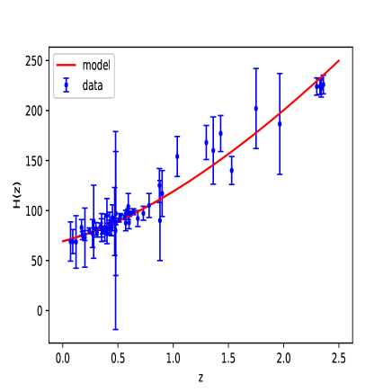
Figure 1: The figure shows the comparison of theoretical model with error bar plots of the OHD points

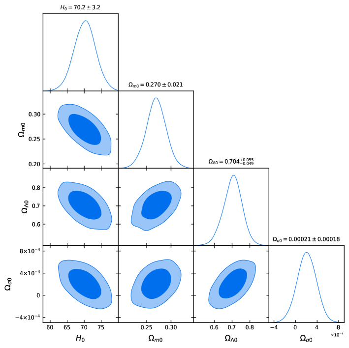
Figure 2: Plots for 1-D marginalized distribution, and 2-D contours with 68$\%$ CL and 95$\%$ CL for the model parameters. Marginalized probability distributions of the individual parameters are also displayed.

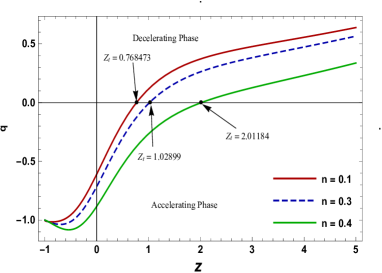
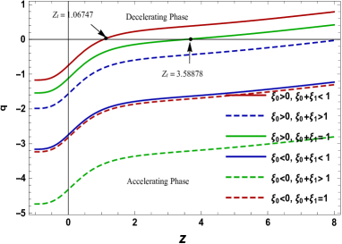
(a) (b) (c) (d)

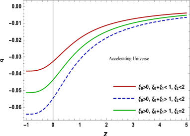
Figure 3: The plots show the behavior of deceleration parameter $q$ versus $z$ for different scenarios. Here $H_{0}=70.2$, $\Omega_{m0}=0.270$, $\Omega_{\Lambda_{0}}=0.704$, $\Omega_{\sigma_{0}}0.00021$, and c=0.001.

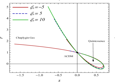
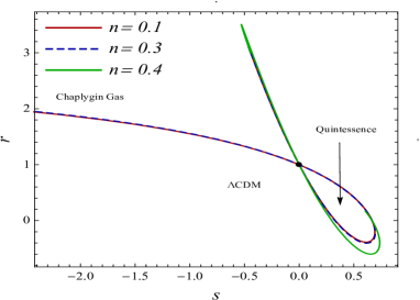
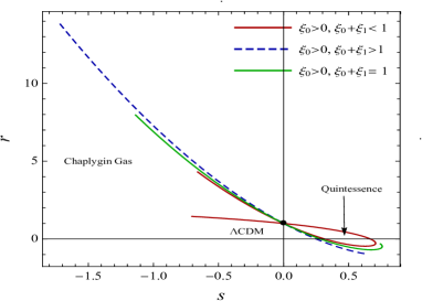
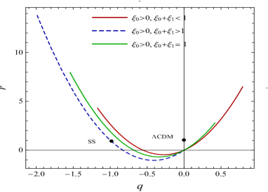
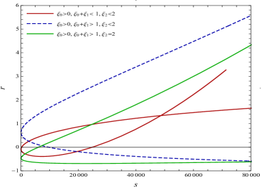
(a) (b) (c) (d) (e) (f) (g) (h)

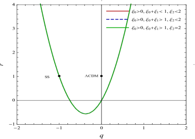
Figure 4: The variations of $r$ versus $s$ are shown in ( figures 4a, 4c, 4e $\&$ 4g). The black dot denotes the statefinder pair $(r,s)=(1,0)$, or the position of a flat $\Lambda$CDM model in the $(r-s)$ plane. The location of statefinder parameters in the best-fitting model based on 57 H(z) data is shown by the star symbol on the $(r-s)$ curve. The variations of $r$ versus $q$ are shown in ( figures 4b, 4d, 4f $\&$ 4h). The black dot represents the location of SS point $(r,q)=(1,-1)$ in the $r–q$ plane, In both panels, we have used four bulk viscosity parameterizations, here $H_{0}=70.2$, $\Omega_{m0}=0.270$, $\Omega_{\Lambda_{0}}=0.704$, $\Omega_{\sigma_{0}}=0.00021$, and $c=0.001.$

5 Result and Dissussion

We use the 57 OHD points to constrain the free parameters of the model under consideration and perform the MCMC technique using the EMCEE Python module. We determined the best-fit parameters in our derived model by minimising the $\chi^{2}$ for the aforementioned datasets. The relationship between $q$ and $z$ for $\xi=-5,5$ and $10$ is seen in figure 3a. The model demonstrates that the display transitioned smoothly from early $q>0$ to late $q<0$. According to the OHD results, the value of $q$ that is accelerating at the moment is in the range $-1\leq q<0$, which implies a decelerating universe, whereas its “negative” value results in an accelerated universe. The results of the 57 data points in the observed high redshift OHD show that our model transits from an early decelerating to a late accelerating cosmos. For different values of $\xi=-5,5,or10$, we discovered that the early Universe was expanding with positive to negative values of $q$ and that there was a signature flipping at $z_{t}=0.80755.$, $z_{t}=0.94572$ and $z_{t}=1.06415$. We can also observe that $q$ will become -1 in the future when $z$ reaches that value. The DP is a function of redshift. The Universe evolves to the infinite future $(z=-1)$ from an inflationary stage at the infinite past $(z=0)$. The K-matter solution (q = 0) appears to be the centre of the universe’s dynamical plane (DP). We can see from Table-2 above that the Universe normally begins with a slowing down phase before transitioning to a speeding up phase for various values of $\xi$.

Table 2: The behaviour of the evoluation of the universe with transitioning point.

range of $\xi$	Nature of $q$	$z_{t}$	Evoluation of the Universe
“ $-10$	+ve to -ve	0 .59043	decelerating- Acclerating
$-5$	+ve to -ve	0.70886	decelerating- Acclerating
$0$	+ve to -ve	0.82792	decelerating- Acclerating
$5$	+ve to -ve	0.94572	decelerating- Acclerating
$10$	+ve to -ve ”	1.06415	decelerating- Acclerating

Figure 3b shows the nature of $q$ with respect to redshift $z$ for $0\leq n\leq 1/2$. The above Table-3 shows that in various values of $n$, the Universe begins smoothly with the deceleration phase to the accelerating phase. We observe that in the future, when z$\to$ -1, q$\to$ -1.

Table 3: The behaviour of the evoluation of the universe with transitioning point.

range of n	Nature of $q$	$z_{t}$	Evoluation of the Universe
“ $0.1$	+ve to -ve	0.85553	decelerating -Acclerating
$0.2$	+ve to -ve	0.93313	decelerating -Acclerating
$0.3$	+ve to -ve	1.0933	decelerating -Acclerating
$0.4$	+ve to -ve	1.6051	decelerating -Acclerating
$0.5$	+ve to -ve”	1.9079	decelerating -Acclerating

Figure 3c shows the nature of $q$ against redshift $z$ for the limiting conditions of the viscous parameters with $\xi_{0}+\xi_{1}>1$,$\xi_{0}+\xi_{1}<1$ and $\xi_{0}+\xi_{1}=1$. The current deceleration parameter $q_{0}>0$ if $\xi_{0}+\xi_{1}>1$, for $\xi_{0}>0$ and $\xi_{1}>0$ indicates that the universe is currently in the decelerating epoch and will transition to the accelerating phase at some point in future if $\xi_{0}<0$ (see Table 4). We have different types of expansions of the Universe:

• For $q>0$, the expansion of the universe would be deceleration.

• For $q=0$, it would expand at a constant rate.

• If $-1<q>0$, the universe would be accelerating with power-law expansion.

• If $q=-1$, the universe has exponential expansion (also known as de Sitter-expansion)

• If $q<-1$, the universe would be super-exponential expansion.

If the limiting conditions of the viscous parameters with $\xi_{0}<0$ , our model shows only the deceleration phase, no trasition point obtained. In particular, the kinematic method of cosmic data analysis offers clear evidence for the universe’s current acceleration stage, which is independent of the universe’s matter-energy composition and the viability of general relativity.

Table 4: The behaviour of the evoluation of the universe with transitioning point.

range of $\xi$	$\xi_{0}$	$\xi_{1}$	Nature of $q$	$z_{t}$	Evolution of Universe
“ $\xi_{0}>0$, $\xi_{0}$+$\xi_{1}<1.0$	0.8	0.1	+ve to -ve	1.4536	decelerating -Acclerating
$\xi_{0}>0$, $\xi_{0}$+$\xi_{1}>1.0$	0.45	0.65	+ve to -ve	3,5882	decelerating -Acclerating
$\xi_{0}>0$, $\xi_{0}$+$\xi_{1}=1.0$	0.65	0.35	+ve to -ve	7.0663	decelerating -Acclerating
$\xi_{0}<0$, $\xi_{0}$+$\xi_{1}<1.0$	-0.5	1.45	-ve	-	Acclerating
$\xi_{0}<0$, $\xi_{0}$+$\xi_{1}>1.0$	-0.5	2.5	-ve	-	Acclerating
$\xi_{0}<0$, $\xi_{0}+\xi_{1}=1.0$”	-0.5	1.5	-ve	-	Acclerating

Similarly, Figure 3d shows the nature of $q$ against redshift $z$ for the limiting conditions of the viscous parameters $\xi_{0}+\xi_{1}>1$, $\xi_{0}+\xi_{1}<1$ and $\xi_{0}+\xi_{1}=1$. We obtained the current deceleration parameter only in the accelerating phase for all $\xi_{0}$, $\xi_{1}$, and $\xi_{2}$. The negative sign indicates inflation (see Table 5).

Table 5: The behaviour of the evoluation of the universe with transitioning point.

range of $\xi$	$\xi_{0}$	$\xi_{1}$	$\xi_{2}$	Nature of $q$	$z_{t}$	Evolution of the universe
“$\xi_{0}>0$, $\xi_{0}$+$\xi_{1}<1.0,\xi_{2}<2.0$	0.9	.01	1	-ve	-	Acclerating
$\xi_{0}>0$,$\xi_{0}$+$\xi_{1}>1.0,\xi_{2}<2.0$	0.45	0.65	1	-ve	-	Acclerating
$\xi_{0}>0$,$\xi_{0}$+$\xi_{1}=1.0,\xi_{2}<2.0$	0.65	.35	1	-ve	-	Acclerating
$\xi_{0}>0$, $\xi_{0}$+$\xi_{1}<1.0,\xi_{2}>2.0$	-0.5	1.45	2.1	-ve	-	Acclerating
$\xi_{0}<0$,$\xi_{0}$+$\xi_{1}>1.0,\xi_{2}>2.0$	-0.5	2.5	3	-ve	-	Acclerating
$\xi_{0}<0$,$\xi_{0}+\xi_{1}>1.0,\xi_{2}>2.0$ ”	-0.5	1.5	2.17	-ve	-	Acclerating

The $r-s$ trajectories in Fig. 4a are separated into two sections by a vertical line. According to references[74, 75], the region $r>1$, $s<0$ in the $r-s$ plane exhibits behavior resembling a Chaplygin gas (CG) model, while the region $r<1$, $s>0$ exhibits behavior resembling the quintessence model (Q-model). The trajectories in all regions coincide for all values of viscous parameter $\xi$, whether positive or negative. The current values of ${r,s}$ (to meet) the $\Lambda$ CDM point for various values of $\xi_{0}$”. Fig 4b shows the behavior of the model in the $(r-q)$ plane. The trajectories are plotted for $\xi=-5,5,10$, and the dot represents the $\Lambda$ CDM point (see Table-6, case I).

Table 6: A numerical description of cosmological model parameters

range of $\xi$	$q$	r	s
$-10$	-0.203426	-0.281664	0.607344
$-5$	-0.302147	-0.299041	0.539818
$0$	-0.400869	-0.23845	0.458243
$5$	-0.49959	-0.099892	0.366781
$10$	-0.598311	0.116633	0.268098

In the case of II, our II parameterization is based on the density parameter. In this case, Fig. 4c  also shows the behavior similar to a CG region, whereas the region $r<1$, $s>0$ depicts the Q-model for $0\leq n<1/2$. The trajectory $r-s$ shows the Q-model early and approaches $\Lambda$CDM at late times. It also shows the CG at early times and approaches $\Lambda$ CDM at late times. Fig. 4d depicts that our model approaches $\Lambda$CDM model. All the trajectories coincide for all different values of $\xi$ (see Table-7, case II).

Table 7: A numerical description of cosmological model parameters

range of n	$q$	r	s
0.1	-0.639804	0.230912	0.224918
0.2	-0.979166	1.68256	-0.153816
0.3	-1.80053	9.00947	-1.16053
0.4	-3.78847	49.0818	-3.73729
0.5	-8.5999	276.928	-10.1074

The case-III shows the nature of $r-s$ and $r-q$ for the limiting conditions of the viscous parameters with $\xi_{0}+\xi_{1}>1$,$\xi_{0}+\xi_{1}<1$ and $\xi_{0}+\xi_{1}=1$. The current deceleration parameter $q_{0}>0$ if $\xi_{0}+\xi_{1}>1$, for $\xi_{0}>0$ and $\xi_{1}>0$ shown in Fig 4e. $\&$ Fig. $4f$ The trajectory shows the Q-model behavior at early times for $\xi_{0}>,\xi_{1}>0$ and approaches $\Lambda$CDM at late times. In both figures the “dot represents the fixed points (r, q) = (1, 0) and (r, q) = (1,-1) of LCDM and Steady State (SS) models”, respectively. It can be observed that there is a sign change of $q$ from positive to negative in a Q-region at small values of $\xi_{0}$ and $\xi_{1}$. The q-factor has always negative values starting from $q<-1$ and tends to $q=-1$ at late times for large values of $\xi_{0}$ and $\xi_{1}$ (see Table-8, case-III).

Table 8: A numerical description of cosmological model parameters

range of $\xi$	$\xi_{0}$	$\xi_{1}$	$q$	$r$	$s$
“ $\xi_{0}>0$, $\xi_{0}+\xi_{0}<1.0$	0.8	0.1	-0.56666	0.03873	0.30039
$\xi_{0}>0$, $\xi_{0}$+$\xi_{1}>1.0$	0.45	0.65	-1.38475	4.62605	-0.64129
$\xi_{0}>0$, $\xi_{0}$+$\xi_{1}=1.0$	0.65	0.35	-0.93870	1.46109	-0.10683
$\xi_{0}<0$, $\xi_{0}$+$\xi_{1}<1.0$	-0.5	1.45	-2.5659	20.6965	-2.1413
$\xi_{0}<0$, $\xi_{0}$+$\xi_{1}>1.0$	-0.6	2.5	-4.13902	59.42716	-4.19823
$\xi_{0}<0$, $\xi_{0}+\xi_{1}=1.0$ ”	-0.7	1.7	-2.93704	28.0484	-2.62322

Similarly, Fig. $4g$ depicts the evolution of our model in the $r-s$ plane. The $r-s$ and $r-q$ planes the trajectory shows the Q-model behavior at early times for and approaches $\Lambda$CDM at late times for the limiting conditions of the viscous parameters $\xi_{0}+\xi_{1}>1$,$\xi_{0}+\xi_{1}<1$ and $\xi_{0}+\xi_{1}=1$, for $\xi_{0}>0,\xi_{1}>0,\xi_{2}>0$. In Fig. 4h the region $r>1$, $q<-1$ in the $r-q$ plane shows a behavior similar to the phantom model (see Table-9, case-IV).

Table 9: A numerical description of cosmological model parameters

range of $\xi$	$\xi_{0}$	$\xi_{1}$	$\xi_{2}$	$q$	$r$	$s$
“ $\xi_{0}>0$, $\xi_{0}$+$\xi_{1}<1.0,\xi_{2}<2.0$	0.9	.01	1	-0.020112	8753.38	-61.348
$\xi_{0}>0$,$\xi_{0}$+$\xi_{1}>1.0,\xi_{2}<2.0$	0.45	0.65	1	-0.020113	8756.63	-61.360
$\xi_{0}>0$,$\xi_{0}$+$\xi_{1}=1.0,\xi_{2}<2.0$	0.65	.35	1	-0.020036	8590.46	-60.7656
$\xi_{0}>0$, $\xi_{0}$+$\xi_{1}<1.0,\xi_{2}>2.0$	-0.5	1.45	2.1	-0.04218	38586.56	-129.9275
$\xi_{0}<0$,$\xi_{0}$+$\xi_{1}>1.0,\xi_{2}>2.0$	-0.5	2.5	3	-0.06033	79415.51	-186.841
$\xi_{0}<0$,$\xi_{0}+\xi_{1}>1.0,\xi_{2}>2.0$”	-0.5	1.5	2.17	-0.04358	41200.78	-134.290

6 Conclusion

As we all know, bulk viscosity is a very important part of cosmology. It helps explain why the universe expands quickly during the inflationary phase. The impact of viscosity on the evolution of cosmological models and the role of viscosity in avoiding the first big bang singularity have been examined by a number of authors [13, 14, 15]. In this study, we examine the Bianchi type-I model with bulk viscosity and the role of bulk viscosity in explaining the early and late universe. The model incorporates the ideal fluid with the four forms of bulk viscosity parameterization. We have performed a detailed study of the Bianchi-I viscous model. We have estimated values of cosmological parameters from the OHD data sets. We have studied four cases of parameterization.

We have provided a summary of the key findings:

• Fig. 1 shows the 2-dimensional joint contours (57 OHD), at 68$\%$and 95$\%$ confidence regions, bounded with latest. We have find the constraint on $H_{0}$, $\Omega_{\text{m0}}$ $\Omega_{\Lambda_{0}},$$\Omega_{\sigma_{0}}$ by (57 OHD ) data sets (Table-I). The best fit values $H_{0}$ are closer to other investigation.

• The error bar plots for OHD data sets are shown in Fig. 2. The dots in both graphs reflect the observed values after corrections, and the red lines compare the current model to the $\Lambda$CDM model, which is depicted by the black dashed lines.

• As shown in the graph, the deceleration parameter $q$ oscillates with $z$ from positive to negative values. The generated model describes the transition from the early deceleration phase to the current expanding phase of the universe. Various viscosity parameterizations for cases I, II, and III are displayed in Figs. $3a,$3b, $3c,and$3d. We also observed that q$\to$ -1 in the future when z$\to$ -1. In case of IV, we obtained the current deceleration parameter only in accelerating phase for all $\xi_{0}$, $\xi_{1}$ and $\xi_{2}$. We can say that the plot of $q$ versus $z$ exhibits cosmic deceleration for high redshift $z$, acceleration for low redshift. We observe that variation of $q$ with bulk viscous coefficient $\xi$ and the model paramters $H_{0}=70.2\pm 3.2$, $\Omega_{\text{m0}}=.270\pm 0.021$, $\Omega_{\Lambda_{0}}=0.704^{+0.055}_{-0.049},$ $\Omega_{\sigma_{0}}=0.00021\pm 0.00018$ have shown in Table $2$, $3$ , $4$ and $5$. The dynamics of the deceleration parameter exhibits a signature transitioning from an early phase of decelerating to the phase in which it is now accelerating. Different studies show transition redshifts as $z_{t}={0.69}^{+0.09}_{-0.06},{0.65}^{+0.10}_{-0.07}$ and ${0.61}^{+0.12}_{-0.08}$ within $(1\sigma)$ for the joined $(SNIa+CC+H_{0})$ data, $z_{t}={0.646}^{+0.020}_{-0.158}$, $z_{t}={0.659}^{+0.371}_{-0.124}$, $z_{t}={0.860}^{+0.013}_{-0.146}$, $z_{t}={1.183}^{+0.002}_{-0.032}$ for SN, OHD and BAO data and $z_{t}={0.8596}^{+0.2886}_{-0.2722}$, $z_{t}={0.6320}^{+0.1605}_{-0.1403}$, and $z_{t}={0.7679}^{+0.1831}_{-0.1829}$ for the models using SNIa, OHD and combined data [91, 92, 93, 94, 95]. Thus, results in the present manuscript show a agreement with the recent analysis.

• We also observed the $(r~{}s)$ and $(r~{}q)$ plane parameters to diagnose the DE model geometrically, as shown in Figs. 4a,4c,4e $\&$ 4f . Our derived model initially shows a Chaplygin gas (CG) type DE model, which later evolves into a quintessence DE model at a few points. The model, later on, reverts again to CG. Interestingly, the model deviates significantly from the point $(r~{}s)=(1,0)$, which coincides with $\Lambda CDM$ see Figs. 4b, 4d, 4e $\&$ 4g for four viscosity parameterization.The detail study of trajectories are shown in Tables 6, 7, 8, 9 for the constrained value of the model parameters $H_{0}=70.2\pm 3.2$, $\Omega_{\text{m0}}=.270\pm 0.021$, $\Omega_{\Lambda_{0}}=0.704^{+0.055}_{-0.049},$ $\Omega_{\sigma_{0}}=0.00021\pm 0.00018$.

We have now come to the conclusion that bulk viscosity can be used to explain DE phenomena.

References

- [1] A. G. Riess,et al., Observational evidence from supernovae for an accelerating universe and a cosmological constant, Astron. J. 116 (1998) 1009.
- [2] S. Perlmutter, G. Aldering, and G. Goldhaber, Measurements of and from 42 high-redshift supernovae, Astron. J. 517 (1999) 565.
- [3] P. A. R. Ade et al., Planck collaboration XV, planck 2013 results. XV. CMB power spectra and likelihood, Astron. Astrophys. 571 (2014) A15.
- [4] P. A. R. Ade et al., Results. XI. CMB power spectra, likelihoods and robustness of parameters, Astron. Astrophys. 594 (2015) A11.
- [5] L. Pogosian and T. Vachaspati, Cosmic microwave background anisotropy from wiggly strings, Phys Rev D 60 (1999) 8.
- [6] P. A. R. Ade et al., Planck Collaboration XVII, Planck 2013 results. XVII. Gravitational lensing by large-scale structure, Astron. Astrophys. 571 (2013) A17.
- [7] P. A. R. Ade et al., Planck 2015 cosmological results Planck Collaboration XV, Planck 2015 results. XV. Gravitational lensing, Astron. Astrophys. 594 (2016) A15.
- [8] C. Eckart, The thermodynamics of irreversible processes. III. Relativistic theory of the simple fluid, Phys. Rev. 58 (1940) 919.
- [9] L. D Landau and E. M Lifshitz, Fluid mechanics Butterworth Heinemann, New York, 1987.
- [10] W. Israel, Nonstationary irreversible thermodynamics: a causal relativistic theory,Ann. Phys. 100 (1976) 310 .
- [11] W. Israel and J. M. Stewart, Thermodynamics of nonstationary and transient effects in a relativistic gas,Phys. Lett. 58 (1976) 213.
- [12] G. L. Murphy, Big-bang model without singularities, Phys. Rev. D 8 (1973) 4231.
- [13] W. H. Huang, Bianchi type I cosmological model with bulk viscosity, Phys. Lett. A 129 (1998) 429 .
- [14] V. K Bhardwaj, M. K. Rana, A. K Yadav, Bulk viscous Bianchi-V cosmological model within the formalism of gravity, Astrophys. Space Sci. 364 (2019) 1.
- [15] A. Dixit, R. Zia, A. Pradhan, Anisotropic bulk viscous string cosmological models of the Universe under a time-dependent deceleration parameter, Pramana-J. Phys. 94 (2020) 1.
- [16] S. J. K. Pacif, Dark energy models from a parametrization of H: a comprehensive analysis and observational constraints Eur. Phys. J. C 135 (2020) 1.
- [17] M. Xin-He and D. Xu, Friedmann cosmology with bulk viscosity: a concrete model for dark energy, Commun. Theor. Phys. 52 (2009) 377.
- [18] C. P. Singh, Bulk viscous cosmology in early universe, Pramana-J. Phys. 71 (2008) 33.
- [19] R. Solanki, S. K. J. Pacif, A. Parida and P. K. Sahoo, Cosmic acceleration with bulk viscosity in modified gravity, Phys. Dark Univ. 32 ( 2021) 100820.
- [20] Y. D. Xu , Z. G. Haaung and X. H. Zhef, Generalized chaplygin gas model with or without viscosity in the plane, Astrophy. Space Sci. 337 (2012 ) 493 .
- [21] C. J. Feng and X. Z. Li, Viscous Ricci dark energy, Phys, Lett. B 680 (2009) 355.
- [22] M. Cataldo, N. Cruz and S. Lepe, Viscous dark energy and phantom evolution, Phys. Lett. B 619 (2005) 5 .
- [23] N. Carlevaro and G. Mod. Montani, Bulk viscosity effects on the early universe stability, Phys. Lett. A 20 (2005) 1729.
- [24] G. Gadbail, S. Arora and P. K. Sahoo, Power-law cosmology in Weyl-type f (Q, T) gravity, Eur. Phys. J. Plus 136 (2021) 1040.
- [25] G. K. Goswami, A. K. Yadav, B. Mishra and S. K. Tripathy, Modeling of accelerating universe with bulk viscous fluid in Bianchi V space‐time, Fortschr. Phys. 69 (2021) 2100007.
- [26] S. Kotambkar, R. K. Kelkar and G. P. Singh, Dynamical behaviours of Chaplygin gas, cosmological and gravitational ’constants’ with cosmic viscous fluid in Bianchi type V space-time geometry, J. Phys. Conf. Ser. 1913 (2021) 012103.
- [27] T. Delubac et al., Baryon acoustic oscillations in the Ly forest of BOSS quasars, Astron. Astrophys. 552 (2013) A96.
- [28] H. Lin, C. Hao, X. Wang, Q. Yuan, Z. L. Yi, T. J. Zhang and B. Q. Wang, Observational data as a complementarity to other cosmological probes, Mod. Phys. Lett. A 24, (2009) 1699.
- [29] J. Simon, L. Verde and R. Jimenez, Constraints on the redshift dependence of the dark energy potential, Phys. Rev. D 71 (2005) 123001.
- [30] O. Farooq, Observational constraint on dark energy cosmological model parameters, Kansas State University PhD Thesis [arXiv:1309.3710] (2013).
- [31] M. Moresco et al. A 6 measurement of the Hubble parameter at : direct evidence of the epoch of cosmic re-acceleration JCAP 014 (2016) 1605 .
- [32] O. Akarsu, T. Dereli and S. Kumar, Probing kinematics and fate of the Universe with linearly time-varying deceleration parameter, Eur. Phys. J. Plus 129 (2014) 1.
- [33] S. Capozziello et al., Cosmic acceleration from a single fluid, Phys. Dark Univ. 20 (2018) 1.
- [34] C. Escamilla-Rivera, M.A.C. Quintero, S. Capozziello, A deep learning approach to cosmological dark energy models, JCAP
- [35] L. Samushia and B. Ratra, Cosmological constraints from Hubble parameter versus redshift data, ApJ 650 (2006) L5.
- [36] B. D Pandey, Pankaj and U. K Sharma, Phantom model for Tsallis Holographic Dark Energy Int. J. Geom. Methods Mod. Phys. 19 (2022) 2250215.
- [37] C. Gruber and O. Luongo, Cosmographic analysis of the equation of state of the universe through Pade approximations, Phys. Rev. D 89 (2014) 103516.
- [38] K. Bamba, Cosmological investigations of (extended) nonlinear massive gravity schemes with nonminimal coupling, Phys. Rev. D 89 (2014) 083518.
- [39] M. Forte, On extended sign-changeable interactions in the dark sector, Gen. Rel. Grav. 46 (2014) 1811.
- [40] S. Capozziello, O. Farooq and O. Luongo, Cosmographic bounds on the cosmological deceleration-acceleration transition redshift in gravity, Phys. Rev. D 90 (2014) 044016.
- [41] R. Y. Guo and X. Zhang, Constraining dark energy with Hubble parameter measurements: an analysis including future redshift-drift observations, Eur. Phys. J. C 76 (2016) 163.
- [42] S. Capozziello, et al., Addressing the cosmological tension by the Heisenberg uncertainty, Found. Phys. 50 (2020) 893.
- [43] S. Capozziello, et al., Thermodynamic parametrization of dark energy, Phys. Dark Univ. 36 (2022) 101045.
- [44] L. Verde, P. Protopapas and R. Jimenez, The expansion rate of the intermediate universe in light of Planck, Phys. Dark Univ. 5 (2014) 307.
- [45] Y. Chen, S. Kumar and B. Ratra, Determining the Hubble constant from Hubble parameter measurements, Astrophys J. 835 (2017) 86.
- [46] Y. Chen and B. Ratra, Hubble parameter data constraints on dark energy, Phys. Lett. B 703(4) (2011) 406.
- [47] R. Nagpal, S. K. J. Pacif, J. K. Singh, K. Bamba and A. Beesham, Analysis with observational constraints in -cosmology in f (R, T) gravity, Eur. Phys. J. C 78, (2018) 1.
- [48] J. Hu and H. Hu, Viscous universe with cosmological constant, Eur. Phys. J. Plus 135, (2020) 1.
- [49] C. Blake, The WiggleZ Dark Energy Survey: Joint measurements of the expansion and growth history at , Mem. R. Astron. Soc. 425 (2012) 405.
- [50] A. K. Yadav, L. K. Sharma, B. K. Singh, and P. K. Sahoo, Existence of bulk viscous universe in f (R, T) gravity and confrontation with observational data, New Astron. 78 (2020) 101382.
- [51] S. Alam et al., The clustering of galaxies in the completed SDSS-III Baryon Oscillation Spectroscopic Survey: cosmological analysis of the DR12 galaxy sample, Mon. Not. R. Astron. Soc. 470 (2017) 2617.
- [52] O. Farooq, S. Crandall and B. Ratra, Binned Hubble parameter measurements and the cosmological deceleration-acceleration transition, Phys. Lett. B 726 (2013) 72.
- [53] J. F. Jesus, R. L. F. Holanda and S. H. Pereira, Model independent constraints on transition redshift, JCAP 05 (2018) 073.
- [54] V. C. Busti, C. Clarkson and M. Seikel, Evidence for a lower value for from cosmic chronometers data ? Mon. Not. R. Astron. Soc. 441 L11.
- [55] Y. Wang, L. Xu and G. B. Zhao, A measurement of the Hubble constant using galaxy redshift surveys, Astrophys J 849 (2017) 84.
- [56] S.Ganjizadeh, A. Amani and M. A. Ramzanpour, Observational Hubble parameter data constraints on the interactive model of gravity with particle creation, Chin. Phys. C 46 (2022), 125104.
- [57] C. Clarkson, B. Bassett and T. H.C. Lu, A general test of the Copernican Principle, Phys Rev Lett 101 (2008) 011201.
- [58] C. Clarkson, M. Cortes and B. Bassett, Dynamical dark energy or simply cosmic curvature? JCAP 08 (2007) 011.
- [59] K. Bamba, S. Capozziello, S. Nojiri and S. D. Odintsov, Dark energy cosmology: the equivalent description via different theoretical models and cosmography tests, Astrophysics and Space Science 342(1) (2012) 155.
- [60] N. Godani, FRW cosmology in gravity, Int. J. Geom. Methods Mod. Phys. 16 (2019) 1950024
- [61] C. P. Singh and P. Kumar, Friedmann model with viscous cosmology in modified gravity theory, Eur. Phys. J. C 74 (2014) 3070.
- [62] C. P. Singh and A. Kumar, Holographic Ricci dark energy with constant bulk viscosity in gravity, Grav. Cos. 25 (2019) 58.
- [63] A. K. Yadav, A. M. Alshehri, N. Ahmad, G. K. Goswami and M. Kumar, Transitioning universe with hybrid scalar field in Bianchi I space–time, Phys. Dark Univ. 31 (2021) 100738.
- [64] J. K Singh S. Rani, Spatially Homogeneous Bianchi Type-I Universes with Variable and , Int. J. Theor. Phys. 52 (2013) 3737.
- [65] O. Heckmann and E. Schucking, Relativistic cosmology in gravitation: An introduction to current research, Willey, New York Chap XI (1962) 438
- [66] G. F. R. Ellis and M. A. H. MacCallum, A class of homogeneous cosmological models, Commun. Math. Phys. 12 (1969) 108.
- [67] V. B. Johri and G. K. Goswami, Spatially homogeneous and anisotropic cosmological models in Brans-Dicke theory, Aust, J. Phys. 34 (1981) 261.
- [68] V. K. Bhardwaj, A. Dixit, R. Rani, G. K Goswami and A. Pradhan, An Axially Symmetric Transitioning models with observational constraints, Chin. J. Phys. 80 (2022) 261.
- [69] S. Ghaffari, A. Sheykhi and M. H. Dehghani, Statefinder diagnosis for holographic dark energy in the DGP braneworld, Phys. Rev. D 91 (2015) 023007.
- [70] V. Sahni T. D. Saini, A. A. Starobinsky and U. Alam, Statefinder-a new geometrical diagnostic of dark energy, J. Exp. Theor. Phys. 77 (2003) 201.
- [71] H. Moradpour, A. H. Ziaie, I. P. Lobo, J. P. M Graca, U. K Sharma and A.S Jahromi, The third law of thermodynamics, non-extensivity and energy definition in black hole physics,Mod. Phys. Lett. A 37 (2020) 2250076.
- [72] J. K. Singh, R. Nagpal, S. K. J. Pacif, Statefinder diagnostic for modified Chaplygin gas cosmology in f (R, T) gravity with particle creation, Int. J. Geom. Methods Mod. Phys. 15 (2018) 1850049.
- [73] R. Myrzakulov and M. Shahalam, Statefinder hierarchy of bimetric and galileon models for concordance cosmology, J. Cosm. Astropart. Phys. 1310 (2013) 047.
- [74] C.P. Singh and M. Srivastava, Viscous cosmology in new holographic dark energy model and the cosmic acceleration, Eur. Ohys. J. C. 78 (2018) 190.
- [75] X. H. Meng and X. Duo, Singularities and entropy in bulk viscosity dark energy model, Commun. Theor. Phys. 56 (2011) 957.
- [76] V. A Belinski and M. I. Khalatnikov, Influence of viscosity on the character of cosmological evolution, J. Exp. Theor. Phys. 42 (1975) 205.
- [77] D. Stern et al., Cosmic chronometers: constraining the equation of state of dark energy. I: H(z) measurements, J. Cosmol. Astropart. Phys. 02 (2010) 008.
- [78] J. Simon, L. Verde and R. Jimenez, Constraints on the redshift dependence of the dark energy potential, Phys. Rev. D 71 (2005) 123001.
- [79] M. Moresco et al., Improved constraints on the expansion rate of the Universe up to from the spectroscopic evolution of cosmic chronometers, J. Cosmol. Astropart. Phys. 08 (2012) 006.
- [80] C. Zhang et al., Four new observational data from luminous red galaxies in the Sloan Digital Sky Survey data release seven, Res. Astron. Astrophys. 14 (2014) 1221.
- [81] A. L. Ratsimbazafy et al., Age-dating luminous red galaxies observed with the Southern African Large Telescope, Mon. Not. Roy. Astron. Soc. 467 (2017) 3239.
- [82] M. Moresco, Raising the bar: new constraints on the Hubble parameter with cosmic chronometers at , Mon. Not. Roy. Astron. Soc. 450 (2015) L16.
- [83] E. Gaztanaga, A. Cabre and L. Hui, Clustering of luminous red galaxies-IV. Baryon acoustic peak in the line-of-sight direction and a direct measurement of , Mon. Not. Roy. Astron. Soc. 399 (2009) 1663.
- [84] A. Oka, S. Saito, T. Nishimichi, A. Taruya and K. Yamamoto, Simultaneous constraints on the growth of structure and cosmic expansion from the multipole power spectra of the SDSS DR7 LRG sample, Mon. Not. Roy. Astron. Soc. 439 (2014) 2515.
- [85] C. H. Chuang and Y. Wang, Modelling the anisotropic two-point galaxy correlation function on small scales and single-probe measurements of , and f(z) (z) from the Sloan Digital Sky Survey DR7 luminous red galaxies, Mon. Not. Roy. Astron. Soc. 435 (2013) 255.
- [86] C. H. Chuang et al., The clustering of galaxies in the SDSS-III Baryon Oscillation Spectroscopic Survey: single-probe measurements and the strong power of f(z) on constraining dark energy, Mon. Not. Roy. Astron. Soc. 433 (2013) 3559.
- [87] L. Anderson et al., The clustering of galaxies in the SDSS-III Baryon Oscillation Spectroscopic Survey: baryon acoustic oscillations in the Data Releases 10 and 11 Galaxy samples, Mon. Not. Roy. Astron. Soc. 441 (2014) 24.
- [88] J. E. Bautista et al., Measurement of baryon acoustic oscillation correlations at with SDSS DR12 Ly-Forests, Astron. Astrophys 603 (2017) A12.
- [89] T. Delubac et al., Baryon acoustic oscillations in the Ly forest of BOSS DR11 quasars, Astron. Astrophys. 574 (2015) A59.
- [90] A. Font-Ribera et al., Quasar-Lyman forest cross-correlation from BOSS DR11: Baryon Acoustic Oscillations, J. Cosmol. Astropart. Phys. 05 (2014) 027.
- [91] R. Nair et al., Cosmokinetics: a joint analysis of standard candles, rulers and cosmic clocks, J. Cosmol. Astropart. Phys. 01 (2012) 018.
- [92] J. Magana et al., Cosmic slowing down of acceleration for several dark energy parametrizations, J. Cosmol. Astropart. Phys. 10 (2014) 017.
- [93] A.A. Mamon, K. Bamba, S. Das, Constraints on reconstructed dark energy model from SN Ia and BAO/CMB observations, Eur. Phys. J. C 77 (2017) 29.
- [94] S. Capozziello, et al., Model-independent reconstruction of cosmological accelerated-decelerated phase, Mon. Not. R. Astron. Soc. 509 (2022) 5399.
- [95] A. A. Mamon, Constraints on a generalized deceleration parameter from cosmic chronometers, Mod. Phys. Lett. A 33 (2018) 1850056.