DDIPNet and DDIPNet+: Discriminant Deep Image Prior Networks for Remote Sensing Image Classification

Abstract

Research on remote sensing image classification significantly impacts essential human routine tasks such as urban planning and agriculture. Nowadays, the rapid advance in technology and the availability of many high-quality remote sensing images create a demand for reliable automation methods. The current paper proposes two novel deep learning-based architectures for image classification purposes, i.e., the Discriminant Deep Image Prior Network and the Discriminant Deep Image Prior Network+, which combine Deep Image Prior and Triplet Networks learning strategies. Experiments conducted over three well-known public remote sensing image datasets achieved state-of-the-art results, evidencing the effectiveness of using deep image priors for remote sensing image classification.

Index Terms—  Remote sensing, Deep Image Prior, Triplet Networks, DDIPNet, DDIPNet+

1 Introduction

Technological advances toward remote sensing provided a large amount of high-quality imagery data, depicting a detailed overview from the Earth’s surface through spatial and spectral resolutions [1]. In a nutshell, such images comprise essential information regarding the land cover, such as rural areas, residential housing, commercial buildings, and vegetation, which is imperative in many real-world problems, e.g., agriculture and city planning.

However, proper segmentation and classification of those regions denote exhausting and cumbersome human tasks, but not for computers. Ulyanov et al. [2] proposed the Deep Image Prior (DIP) approach recently, which employs a generator network to capture low-level image information before any sample-based learning. Besides, Liu et al. [3] proposed the triplet networks, a model that employs weakly labeled images to alleviate the necessity of a massive volume of labeled samples for training.

This paper proposes two deep learning approaches, i.e., the Deep Image Prior Network (DDIPNet) and the Discriminant Deep Image Prior Network+ (DDIPNet+), which combine DIP modeling and triplet networks strategies with remote sensing image classification. Therefore, the main contributions of this paper are threefold:

• to propose two hybrid deep neural network models, i.e., DDIPNet and DDIPNet+;

• to provide a novel approach for remote sensing image classification; and

• to foster the literature concerning both deep learning and remote sensing image classification.

The remainder of this paper is presented as follows. Section 2 provides the theoretical background concerning DDIPNet and DDIPNet+. Further, Sections 3 and 4 describe the methodology and the experimental results, respectively. Finally, Section 5 states the conclusions and future works.

2 Proposed Approach

This section describes DDIPNet and DDIPNet+ architectures, two novel approaches for remote sensing image classification. The models comprise a projective convolutional neural network (VGG16), a Deep Convolutional Generative Prior Network (DCGPN), and a triplet loss function. The difference between DDIPNet and DDIPNet+ stands in the optimization step, in which DDIPNet+ incorporates data augmentation into its triplet network optimization process. Figure 1 depicts the general idea of the models.

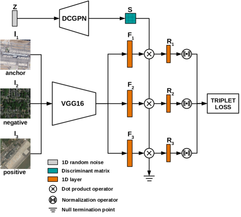
Fig. 1: DDIPNet and DDIPNet+ joint optimization architecture configuration.

Given a set of input images ${\cal{I}}=\{\bm{I}_{1},\bm{I}_{2},\bm{I}_{3}\}$ such that $\bm{I}_{1}$ and $\bm{I}_{2}$ stand for the anchor and negative examples, respectively, and $\bm{I}_{3}$ denotes the positive sample, the VGG16 neural network is employed to project each of those images into a set of its corresponding low-level feature domain representations ${\cal F}=\{\bm{F}_{1},\bm{F}_{2},\bm{F}_{3}\}$. In this work, we considered $\bm{I}_{j}\in\mathbb{R}^{224\times 224}$ and $\bm{F}_{j}\in\mathbb{R}_{+}^{1\times f}$, where $f=4,096$ stands for VGG16’s last fully connected layer dimension, $\forall j\in\{1,2,3\}$.

Given a random uniform distributed input $\bm{Z}\in\mathbb{R}^{1\times 100}$, the DCGPN network is trained to produce a prior generative model, i.e., a discriminant matrix $\bm{S}\in\mathbb{R}^{f\times c}$, where $c$ stands for the number of classes. The matrix $\bm{S}$ is then used to project ${\cal F}$ into a more compact and separable feature domain $\cal{R}$, such that ${\cal R}=\{\bm{R}_{1},\bm{R}_{2},\bm{R}_{3}\}$ and $\bm{R}_{j}\in\mathbb{R}^{1\times c}$, $\forall j\in\{1,2,3\}$. Notice that DCGPN follows its original architecture [4], except for the depth of the last layer, which in this case is equivalent to $c$.

The DDIPNets joint optimization step consists of minimizing a triplet loss function given by:

$$L(D_{1},D_{2};\Theta,\Phi)=max(0,D_{1\{\Theta,\Phi\}}-D_{2\{\Theta,\Phi\}}+m),$$ (1)

where $\Theta$ and $\Phi$ stand for the VGG16 and DCGPN trainable parameters, respectively, and $m=0.5$ denotes the margin constant.

The term $D_{1\{\Theta,\Phi\}}$ denotes the positive pairwise distance between the anchor feature representation $Q(\bm{R}_{1})$ and the same class feature representation $Q(\bm{R}_{3})$, being computed as follows:

$$D_{1\{\Theta,\Phi\}}=\lVert Q(\bm{R}_{1})-Q(\bm{R}_{3})\rVert_{2},$$ (2)

and $D_{2\{\Theta,\Phi\}}$ denotes the negative pairwise distance between the normalized anchor feature representation $Q(\bm{R}_{1})$ and the different class normalized feature representation $Q(\bm{R}_{2})$, being computed as follows:

$$D_{2\{\Theta,\Phi\}}=\lVert Q(\bm{R}_{1})-Q(\bm{R}_{2})\rVert_{2}.$$ (3)

Last but not least, $Q(\cdot)$ stands for the non-linear squashing function [5] and it can be computed as follows:

$$Q(\bm{R}_{j})=\frac{\lVert\bm{R}_{j}\rVert_{2}^{2}}{1+\lVert\bm{R}_{j}\rVert_{2}^{2}}\frac{\bm{R}_{j}}{\lVert\bm{R}_{j}\rVert_{2}},$$ (4)

such that $\forall j\in\{1,2,3\}$.

After VGG16 and DCGPN models have been trained and jointly optimized, the model’s output is employed to feed a linear Support Vector Machine (SVM) classifier, as depicted in Figure 2.

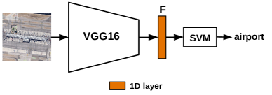
Fig. 2: DDIPNet and DDIPNet+ classification architecture.

3 Methodology

We considered three public remote sensing image datasets for a fair evaluation of the proposed approaches, as described bellow:

• UC-Merced [6]: composed of $21$ classes, each containing $100$ samples of size $256\times 256$ pixels, ending up in $2,100$ images.

• AID [1]: comprises $30$ classes of large-scale aerial scenes totaling $10,000$ images of size $600\times 600$ pixels. The dataset is imbalanced.

• NWPU-RESISC45 [7]: comprises $31,500$ large-scale aerial scene images of size $256\times 256$ equally distributed into $45$ distinct categories.

Following the methodology proposed by Zhang et al. [5], the models are trained and evaluated over two distinct splitting scenarios. Moreover, different ratios are considered for each dataset, i.e., UC-Merced is trained first with $80\%$ of the samples and further $50\%$ of the instances. Regarding AID dataset, the training folds are built using $50\%$ and $20\%$ of the samples, and finally, NWPU-RESISC45 considers $20\%$ and $10\%$ of the samples for training. For statistical purposes, the procedure is performed during $10$ executions, and the average accuracies are computed for each model.

The training steps are performed as follows:

1. Both VGG16 (previously trained over ImageNet) and DCGPN networks are jointly trained during a maximum period of $50$ epochs to minimize Equation (1). The training procedure considers batches of size $32$, Adam optimizer, and learning rates of $10^{-6}$ and $10^{-4}$ assuming VGG16 and DCGPN models, respectively.

2. Further, the VGG16 network projects the training images into a feature domain through its last fully connected layer.

3. A linear Support Vector Machines (SVM) classifier is trained using the projected features as input. Notice the default parameters are used according to Xia et al. [1].

The evaluation process is performed by submitting the test images through the models and measuring the average accuracies obtained in the process.

4 Experimental Results

Table 1 presents the results over UC-Merced dataset concerning the proposed models against some state-of-the-art approaches. Considering the $80\%$ training ratio, DDIPNet overcomes four-out-of-twelve techniques and presented comparable results concerning another three ones. Over the $50\%$ training ratio, it overcame VGG-16, TEX-Net-LF, and VGG-16-CapsNet, in a total of three-out-of-six baselines. Concerning DDIPNet+, one can observe even better results, outperforming eight-out-of-twelve and four-out-of-six baselines considering $80\%$ and $50\%$ training ratios, respectively.

Table 1: Overall accuracies ($\%$), standart deviations, and rank positions in parenthesis considering UC-Merced dataset.

Method	80% Training Ratio	50% Training Ratio
VGG-16 [1]	$95.21\pm 1.20$ $(14)$	$94.14\pm 0.69$ $(8)$
TEX-Net-LF [8]	$96.62\pm 0.49$ $(13)$	$95.89\pm 0.37$ $(6)$
LGFBOVW [9]	$96.88\pm 1.32$ $(12)$	/
Fine-tuned GoogLeNet [10]	$97.10$ $(11)$	/
Fusion by addition [11]	$97.42\pm 1.79$ $(9)$	/
CCP-net [12]	$97.52\pm 0.97$ $(8)$	/
Two-Stream Fusion [13]	$98.02\pm 1.03$ $(7)$	$96.97\pm 0.75$ $(4)$
DSFATN [14]	$98.25$ $(6)$	/
Deep CNN Transfer [15]	$98.49$ $(4)$	/
GCFs+LOFs [16]	$99.00\pm 0.35$ $(2)$	$97.37\pm 0.44$ $(2)$
VGG-16-CapsNet [5]	$98.81\pm 0.22$ $(3)$	$95.33\pm 0.18$ $(7)$
Inception-v3-CapsNet [5]	$\textbf{99.05}\bm{\pm}\textbf{0.22}$ (1)	$\textbf{97.59}\bm{\pm}\textbf{0.16}$ (1)
DDIPNet (ours)	$97.28\pm 0.75$ $(10)$	$96.00\pm 0.70$ $(5)$
DDIPNet+ (ours)	$98.28\pm 0.64$ $(5)$	$97.28\pm 0.58$ $(3)$

Table 2 presents the results over AID dataset. Considering the $50\%$ training ratio, DDIPNet outperformed three-out-of-seven techniques, while DDIPNet+ also obtained better results surpassing five-out-of-seven of them. Similar results were obtained over the $20\%$ training ratio scenario.

Table 2: Overall accuracies ($\%$), standart deviations, and rank positions in parenthesis considering AID dataset.

Method	50% Training Ratio	20% Training Ratio
VGG-16 [1]	$89.64\pm 0.36$ $(9)$	$86.59\pm 0.29$ $(8)$
TEX-Net-LF [8]	$92.96\pm 0.18$ $(7)$	$90.87\pm 0.11$ $(6)$
Fusion by addition [11]	$91.87\pm 0.36$ $(8)$	/
Two-Stream Fusion [13]	$94.58\pm 0.25$ $(5)$	$92.32\pm 0.41$ $(4)$
GCFs+LOFs [16]	$\textbf{96.85}\bm{\pm}\textbf{0.23}$ (1)	$92.48\pm 0.38$ $(3)$
VGG-16-CapsNet [5]	$94.74\pm 0.17$ $(4)$	$91.63\pm 0.19$ $(5)$
Inception-v3-CapsNet [5]	$96.32\pm 0.12$ $(2)$	$\textbf{93.79}\bm{\pm}\textbf{0.13}$ (1)
DDIPNet (ours)	$93.91\pm 0.47$ $(6)$	$89.88\pm 0.49$ $(7)$
DDIPNet+ (ours)	$95.31\pm 0.22$ $(3)$	$92.59\pm 0.52$ $(2)$

Considering NWPU-RESISC45 dataset (Table 3), one can observe that DDIPNet+ was capable of overcoming Fine-tuned VGG-16 and VGG-16-CapsNet considering same training ratios.

Table 3: Overall accuracies ($\%$), standart deviations, and rank positions in parenthesis considering NWPU-RESISC45 dataset.

Method	20% Training Ratio	10% Training Ratio
Fine-tuned VGG-16 [1]	$90.36\pm 0.18$ $(4)$	$87.15\pm 0.45$ $(3)$
Triple networks [3]	$92.33\pm 0.20$ $(2)$	/
VGG-16-CapsNet [5]	$89.18\pm 0.14$ $(5)$	$85.08\pm 0.13$ $(4)$
Inception-v3-CapsNet [5]	$\textbf{92.60}\bm{\pm}\textbf{0.11}$ (1)	$\textbf{89.03}\bm{\pm}\textbf{0.21}$ (1)
DDIPNet (ours)	$88.33\pm 0.43$ $(6)$	$83.67\pm 0.64$ $(5)$
DDIPNet+ (ours)	$91.54\pm 0.31$ $(3)$	$88.14\pm 0.42$ $(2)$

4.1 Discussion

Summarizing Tables 1 to 3, we can highlight that DDIPNet showed better results than pre-trained VGG-16, and also than more complex texture-based and visual word-based techniques, such as TEX-Net-LF and LGFBOVW. Meanwhile, DDIPNet+ surpassed the state-of-the-art CapsNet concerning the same VGG-16 backbone. Besides, DDIPNet+ figures a primary advantage over CapsNet since its DCGPN module and discriminant matrix are not incorporated into the final classifier model, thus being quite faster for prediction.

4.2 Ablation Study

As mentioned earlier in Section 2, the proposed approaches figure the main hyperparameter $m$, i.e., the margin constant. We conducted an ablation study to find out the best value. For the sake of space, we present an ablation study over UC-Merced dataset only. Figure 3 depicts such a study, in which $m=0.5$ showed a suitable choice concerning the trade-off between accuracy and robustness (standard deviation).

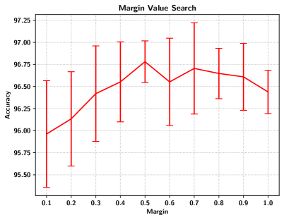
Fig. 3: Margin grid search process conducted over UC-Merced [6] dataset, regarding $50\%$ training samples. We considered margin variations of $0.1$, and the searches were executed by five rounds of $15$ training epochs each.

5 Conclusion

This work proposes two image classification approaches named DDIPNet and DDIPNet+, which combine Deep Image Prior and triplet network optimization strategies to cope with remote sensing image classification. The proposed approaches showed promising results in three public datasets, overcoming state-of-the-art techniques in some situations. Besides, DDIPNet and DDIPNet+ figure a lighter training and classification steps than their counterparts. Regarding future works, we intend to improve DDIPNet and DDIPNet+ thourgh modifications in the VGG-16 backbone.

References

- [1] Gui-Song Xia, Jingwen Hu, Fan Hu, Baoguang Shi, Xiang Bai, Yanfei Zhong, Liangpei Zhang, and Xiaoqiang Lu, “AID: A benchmark data set for performance evaluation of aerial scene classification,” IEEE Transactions on Geoscience and Remote Sensing, vol. 55, no. 7, pp. 3965–3981, 2017.
- [2] Dmitry Ulyanov, Andrea Vedaldi, and Victor Lempitsky, “Deep image prior,” in Proceedings of the IEEE Conference on Computer Vision and Pattern Recognition, 2018, pp. 9446–9454.
- [3] Yishu Liu and Chao Huang, “Scene classification via triplet networks,” IEEE Journal of Selected Topics in Applied Earth Observations and Remote Sensing, vol. 11, no. 1, pp. 220–237, 2017.
- [4] Alec Radford, Luke Metz, and Soumith Chintala, “Unsupervised representation learning with deep convolutional generative adversarial networks,” arXiv preprint arXiv:1511.06434, 2015.
- [5] Wei Zhang, Ping Tang, and Lijun Zhao, “Remote sensing image scene classification using CNN-CapsNet,” Remote Sensing, vol. 11, no. 5, pp. 494, 2019.
- [6] Yi Yang and Shawn Newsam, “Bag-of-visual-words and spatial extensions for land-use classification,” in Proceedings of the 18th SIGSPATIAL international conference on advances in geographic information systems, 2010, pp. 270–279.
- [7] Gong Cheng, Junwei Han, and Xiaoqiang Lu, “Remote sensing image scene classification: Benchmark and state of the art,” Proceedings of the IEEE, vol. 105, no. 10, pp. 1865–1883, 2017.
- [8] Rao Muhammad Anwer, Fahad Shahbaz Khan, Joost van de Weijer, Matthieu Molinier, and Jorma Laaksonen, “Binary patterns encoded convolutional neural networks for texture recognition and remote sensing scene classification,” ISPRS journal of photogrammetry and remote sensing, vol. 138, pp. 74–85, 2018.
- [9] Qiqi Zhu, Yanfei Zhong, Bei Zhao, Gui-Song Xia, and Liangpei Zhang, “Bag-of-visual-words scene classifier with local and global features for high spatial resolution remote sensing imagery,” IEEE Geoscience and Remote Sensing Letters, vol. 13, no. 6, pp. 747–751, 2016.
- [10] Marco Castelluccio, Giovanni Poggi, Carlo Sansone, and Luisa Verdoliva, “Land use classification in remote sensing images by convolutional neural networks,” arXiv preprint arXiv:1508.00092, 2015.
- [11] Souleyman Chaib, Huan Liu, Yanfeng Gu, and Hongxun Yao, “Deep feature fusion for vhr remote sensing scene classification,” IEEE Transactions on Geoscience and Remote Sensing, vol. 55, no. 8, pp. 4775–4784, 2017.
- [12] Kunlun Qi, Qingfeng Guan, Chao Yang, Feifei Peng, Shengyu Shen, and Huayi Wu, “Concentric circle pooling in deep convolutional networks for remote sensing scene classification,” Remote Sensing, vol. 10, no. 6, pp. 934, 2018.
- [13] Yunlong Yu and Fuxian Liu, “A two-stream deep fusion framework for high-resolution aerial scene classification,” Computational intelligence and neuroscience, vol. 2018, 2018.
- [14] Xi Gong, Zhong Xie, Yuanyuan Liu, Xuguo Shi, and Zhuo Zheng, “Deep salient feature based anti-noise transfer network for scene classification of remote sensing imagery,” Remote Sensing, vol. 10, no. 3, pp. 410, 2018.
- [15] Fan Hu, Gui-Song Xia, Jingwen Hu, and Liangpei Zhang, “Transferring deep convolutional neural networks for the scene classification of high-resolution remote sensing imagery,” Remote Sensing, vol. 7, no. 11, pp. 14680–14707, 2015.
- [16] Dan Zeng, Shuaijun Chen, Boyang Chen, and Shuying Li, “Improving remote sensing scene classification by integrating global-context and local-object features,” Remote Sensing, vol. 10, no. 5, pp. 734, 2018.