geepers: Principal Stratification using Principal Scores and Stacked Estimating Equations

Abstract

Principal stratification is a framework for making sense of causal effects conditioned on variables that themselves may have been affected by treatment. Most principal stratification estimators rely on strong structural or modeling assumptions, and many require advanced statistical training to fit and to check. In this paper, we introduce a new M-estimation principal effect estimator for one-way noncompliance based on a binary indicator. Estimates may be computed using conventional regressions (though the standard errors require a specialized sandwich formula) and do not rely on distributional assumptions. We illustrate the new technique in an analysis of student log data from a recent educational technology field experiment.

1 Introduction

Randomized experiments easily admit subgroup analysis—estimation of treatment effects for a subset of the study population—when those subgroups are defined at baseline, and not themselves a function of treatment assignment. However, when subgroup membership is a function of a post-treatment variable, then it may itself be affected by the treatment. Contrasts between treatment and control conditions within those subgroups may not have a causal interpretation at all—and when they do, the same techniques that work for subgroups defined at baseline will often produce inconsistent estimates.

Principal stratification (Frangakis and Rubin, 2002) is a broad framework for defining subgroup effects for post-treatment subgroups. It relies on the notion of potential subgroups called principal strata: groups of subjects defined based on the values a post-treatment variable would potentially take if the subject were assigned to one treatment condition or another. Since principal strata membership is based on subjects’ responses to both factual and counter-factual treatment assignments, it is in general unobserved. Nonetheless, researchers have devised estimators of principal effects, as average effects within principal strata are called, to address a broad range of applied statistical problems, including non-compliance in randomized experiments (Angrist et al., 1996), the evaluation of surrogate outcomes (Li et al., 2010), the investigation of causal mechanisms (Page, 2012), and sample attrition (Zhang and Rubin, 2003; Ding et al., 2011).

Because principal strata membership is generally unobserved, principal effects are not always identified, and when they are, estimation can still be difficult. Typically, principal effects are identified and estimated based on strong structural assumptions (e.g. Angrist et al., 1996) and/or parametric modeling (e.g. Imbens and Rubin, 1997). Parametric models for principal effects are often hard to specify and hard or impossible to test. Even when they are well-specified they can yield estimates that are severely biased and misleading (Griffin et al., 2008; Ho et al., 2022). Another route to identification and estimation of principal effects leads through auxiliary data, including baseline covariates or secondary outcomes (Mattei et al., 2013). Of particular importance is the “principal score,” (Jo and Stuart, 2009; Ding and Lu, 2017; Feller et al., 2017), or the probability that a subject belongs to a particular principal stratum, as a function of pre-treatment covariates. Under a strong, untestable assumption called “principal ignorability,” principal scores can be transformed into weights to compute form an unbiased estimate of principal effects.

On the other hand, Jo (2002), Ding et al. (2011), Jiang and Ding (2021), and others have shown that, under certain circumstances, researchers can use baseline covariates to identify and estimate principal effects without relying on principal ignorability. This paper expands on those identification results by presenting a new set of principal effect estimators, and associated standard error estimates, based on a general estimating equations (or M-estimation or method-of-moments) (Stefanski and Boos, 2002). It turns out that, under certain general conditions, principal effects can be estimated with a simple, two-step procedure: first, estimate principal scores with logistic regression or another M-estimator; then, impute unknown principal subgroup membership indicators with principal scores and estimate principal effects using ordinary least squares (OLS) regression with interactions. We will refer to the estimators presented here as “geepers”: generalized estimating equations for principal effects using regressions. geepers estimates rely on correct specification of regression functions, but unlike common fully-parametric methods, they make no assumptions about the shape of the distribution of regression errors. Unlike principal score weighting, geepers does not assume principal ignorability, and admits to sandwich-style standard error estimates, which we provide in the appendix.

This paper focuses on a special case of principal stratification—one-way, binary non-compliance—that is, there are only two principal strata, and principal stratum membership is observable in one treatment arm, but not in the other. This scenario would occur if, say, subjects in the control arm of a study had no access to the treatment, and not all subjects assigned to the treatment arm actually received the full treatment. While such a setup may represent the simplest and easiest principal stratification problem, we believe it is a common scenario. Moreover, we believe that the methods developed here can extend to more complex scenarios, which we leave to future work.

The following section gives a formal introduction to principal stratification and briefly describes two common estimation techniques, parametric mixture modeling and principal score weighting. Next, Section 3 develops geepers estimation, and gives conditions for its consistency. Section 4 describes a simulation study examining the operating characteristics of geepers estimates and comparing them to estimates from parametric mixture modeling and principal score weighting. Under ideal circumstances, estimates from parametric mixture models and weighting estimators are somewhat more efficient than geepers, but when assumptions are violated geepers easily out-performs the other two methods. Section 5 illustrates geepers in analyzing data from a recent large-scale field trial of educational software, and Section 6 concludes.

2 Background

In a randomized experiment with two conditions, let $Z_{i}=0$ if subject $i$, $i=1,\dots,n$ is assigned to the treatment condition, and let $Z_{i}=0$ otherwise. If interest is in the effect of $Z$ on an outcome $Y$, under the “stable unit treatment value assumption” (Angrist et al., 1996) of no interference between units and no hidden versions of the treatment, define potential outcomes (Splawa-Neyman et al., 1990) $Y_{Ti}$ as the value of $Y$ that $i$ would exhibit if $Z_{i}=1$, and let $Y_{Ci}$ be the value if $Z_{i}=0$. Then the observed value of $Y$ satisfies $Y_{i}=Z_{i}Y_{Ti}+(1-Z_{i})Y_{Ci}$, and the treatment effect of $Z$ on $Y$ for subject $i$ may be defined as $\tau_{i}=Y_{Ti}-Y_{Ci}$. The average treatment effect (ATE) is $\mathbb{E}[\tau]$.

Let $S_{i}\in\{0,1\}$ be a measurement on subject $i$ taken subsequent to treatment assignment, so that $S$ may be affected by $Z$. Then $S$ itself has potential values $S_{Ti}$ and $S_{Ci}$, which $i$ would exhibit if $Z_{i}=1$ or $Z_{i}=0$, respectively. Assume “strong monotonicity” (c.f. Ding and Lu, 2017) (also referred to as “one-way noncompliance”):

Assumption 1 (Strong Monotonicity)

$$S_{Ci}=0\text{ for all }i$$

Like potential outcomes $Y_{Ti}$ and $Y_{Ci}$, $S_{Ci}$ and $S_{Ti}$ are defined for all subjects, though $S_{Ci}$ is only observed when $Z_{i}=0$ and $S_{Ti}$ is only observed when $Z_{i}=1$. Under strong monotonicity, since $S$ is binary, every subject belongs to one of two “principal strata,” $S_{Ti}=1$ or $S_{Ti}=0$. The average treatment effect in each principal stratum, $\tau^{1}=\mathbb{E}[\tau|S_{T}=1]$ or $\tau^{1}=\mathbb{E}[\tau|S_{T}=0]$, is called a principal effect. The challenge in estimating principal effects is due to the fact that strata membership $S_{Ti}$ is only observed when $Z_{i}=1$, in which case $S_{Ti}=S_{i}$, the observed value of $S$.

2.1 Estimating Principal Effects

In estimating principal effects for a binary $S$, it will be useful to define four conditional means. For $s\in\{0,1\}$, let

$$\mu_{C}^{s}=\mathbb{E}[Y_{C}|S_{T}=s]\mbox{ and }\mu_{T}^{s}=\mathbb{E}[Y_{T}|S_{T}=s]$$ (1)

Then, since

$$\tau^{s}=\mu_{T}^{s}-\mu_{C}^{s}$$

estimating principal effects requires estimating the four conditional means.

We will focus on estimation in completely randomized experiments, that is, we will assume

Assumption 2 (Randomization)

$$Y_{Ci},Y_{Ti},S_{Ti},\bm{x}_{i}\mathchoice{\mathrel{\hbox to0.0pt{$\displaystyle\perp$\hss}\mkern 2.0mu{\displaystyle\perp}}}{\mathrel{\hbox to0.0pt{$\textstyle\perp$\hss}\mkern 2.0mu{\textstyle\perp}}}{\mathrel{\hbox to0.0pt{$\scriptstyle\perp$\hss}\mkern 2.0mu{\scriptstyle\perp}}}{\mathrel{\hbox to0.0pt{$\scriptscriptstyle\perp$\hss}\mkern 2.0mu{\scriptscriptstyle\perp}}}Z_{i}$$

where $\bm{x}_{i}$ is a vector of pre-treatment covariates.

Under Assumptions 1 and 2, conditional means $\mu_{T}^{0}$ and $\mu_{T}^{1}$ are nonparametrically identified. In particular, the means of observed outcomes for subjects with $Z=1$ and $S=0$ or $S=1$ are unbiased for $\mu_{T}^{0}$ and $\mu_{T}^{1}$, respectively, since when $Z_{i}=1$, $Y_{i}=Y_{Ti}$ and $S_{i}=S_{Ti}$. In contrast, $\mu_{C}^{0}$ and $\mu_{C}^{1}$ are not fully identified without further assumptions because $S_{Ti}$ and $Y_{Ci}$ are never observed simultaneously (though they may be nonparametrically bounded; see, e.g., Miratrix et al. 2018). We will briefly review two approaches to estimating $\mu_{C}^{0}$ and $\mu_{C}^{1}$—normal mixture modeling and weighting—with some comments in-between on the role for covariates.

2.1.1 Normal Mixture Modeling

The normal mixture modeling approach to estimating $\mu_{C}^{0}$ and $\mu_{C}^{1}$ (Imbens and Rubin, 1997) assumes that, conditional on $S_{T}$, $Y_{C}$ is normally distributed. Then the probability density of $Y_{C}$ may be written as

$$f_{Y_{C}}(y)=Pr(S_{T}=0)\phi\left(\frac{y-\mu_{C}^{0}}{\sigma_{C}^{0}}\right)+Pr(S_{T}=1)\phi\left(\frac{y-\mu_{C}^{1}}{\sigma_{C}^{1}}\right)$$ (2)

where $\phi(\cdot)$ is the standard normal density function, and $\sigma_{C}^{0}>0$ and $\sigma_{C}^{1}>0$ are standard deviations, which are sometimes assumed equal. The probabilities $Pr(S_{T}=0)$ and $Pr(S_{T}=1)$ may be estimated first using data from the treatment group, since Assumption 2 implies that $Pr(S_{T}=1|Z=1)=Pr(S_{T}=1)$. Given these estimates and (2), parameters $\mu_{C}^{0}$ and $\mu_{C}^{1}$ may be estimated using maximum likelihood, method of moments, or Bayesian techniques.

This approach has a number of setbacks. First, the conditional normality assumption is untestable and limiting. Unfortunately, even when it holds, mixture model estimates can be unreliable and, in some cases, severely biased (Griffin et al., 2008; Feller et al., 2017).

2.2 Principal Scores

The principal score (e.g. Jo and Stuart, 2009) is defined as

$$e(\bm{X}^{S}_{i})=Pr(S_{Ti}=1|\bm{X}^{S}_{i})$$ (3)

where $\bm{X}^{S}_{i}\subseteq\bm{x}_{i}$, the set of covariates used to model $S$. Note that under randomization, $Pr(S_{Ti}=1|\bm{X}^{S}_{i},Z_{i})=Pr(S_{Ti}=1|\bm{X}^{S}_{i})$, so a model for principal scores can be estimated using data from the treatment group and extrapolated to the control group. Assume a model for principal scores:

$$e_{\bm{\alpha}}(\bm{X}^{S}_{i})=f(\bm{X}^{S}_{i};\bm{\alpha})$$ (4)

with parameter vector $\bm{\alpha}$. An analyst may estimate $\bm{\alpha}$ by fitting model (4) using observed $\bm{S}$ and $\bm{X}^{S}$ for subjects with $Z=1$, and then compute estimated principal scores $e_{\bm{\hat{\alpha}}}(\bm{X}^{S}_{i})$ for subjects with $Z_{i}=1$.

Going forward, we will occasionally suppress dependence on $\bm{\alpha}$, and write $e_{\bm{\alpha}}(\bm{X}^{S}_{i})=e(\bm{X}^{S}_{i})$.

In order for principal scores to be useful, they need to vary with $\bm{x}$. Otherwise, $\bm{x}$ is uninformative about $S_{T}$. In particular, we will assume the following:

Assumption 3 (Variable Principal Scores)

$e(\bm{X}^{S})$ takes at least 3 distinct values

For a broader discussion, see Ding et al. (2011); Jiang and Ding (2021).

Principal scores can potentially improve inference in a finite mixture model, by re-writing (2) as

$$f_{Y_{C}}(y)=(1-e_{\bm{\alpha}}(\bm{X}^{S}_{i}))\phi\left(\frac{y-\mu_{C}^{0}}{\sigma_{C}^{0}}\right)+e_{\bm{\alpha}}(\bm{X}^{S}_{i})\phi\left(\frac{y-\mu_{C}^{1}}{\sigma_{C}^{1}}\right)$$ (5)

Alternatively, an analyst may assume “principal ignorability” (Jo and Stuart, 2009; Ding and Lu, 2017):

Assumption 4 (Principal Ignorability)

$$Y_{C}\mathchoice{\mathrel{\hbox to0.0pt{$\displaystyle\perp$\hss}\mkern 2.0mu{\displaystyle\perp}}}{\mathrel{\hbox to0.0pt{$\textstyle\perp$\hss}\mkern 2.0mu{\textstyle\perp}}}{\mathrel{\hbox to0.0pt{$\scriptstyle\perp$\hss}\mkern 2.0mu{\scriptstyle\perp}}}{\mathrel{\hbox to0.0pt{$\scriptscriptstyle\perp$\hss}\mkern 2.0mu{\scriptscriptstyle\perp}}}S_{T}|\bm{X}^{S}$$ (6)

or a somewhat weaker version, $\mathbb{E}[Y_{C}|S_{T},\bm{X}^{S}]=\mathbb{E}[Y_{C}|\bm{X}^{S}]$ (Feller et al., 2017). That is, the principal stratum is unrelated to control potential outcomes conditional on covariates. Principal ignorability (6) is reminiscent of ignorability assumptions typical in observational studies. In particular, an unobserved covariate $u$ that is correlated with both $S_{T}$ and $Y_{C}$ would invalidate (6).

Under principal ignorability, $\mu_{C}^{0}$ and $\mu_{C}^{1}$ can be estimated via weighting:

$$\hat{\mu_{C}^{0}}_{w}=\frac{\sum_{i:Z_{i}=0}Y_{i}(1-e(\bm{X}^{S}))}{\sum_{i:Z_{i}=0}1-e(\bm{X}^{S})}\text{ and }\hat{\mu_{C}^{1}}_{w}=\frac{\sum_{i:Z_{i}=0}Y_{i}(e(\bm{X}^{S}))}{\sum_{i:Z_{i}=0}e(\bm{X}^{S})}$$ (7)

Principal score weighting (psw) does not require any distributional assumptions and (after estimating principal scores) is very easy to implement. On the other hand, the principal ignorability assumption is strong and restrictive.

Feller et al. (2017) recommends the case-resampling bootstrap to estimate the sampling variances of $\hat{\mu}_{Cw}^{0}$, $\hat{\mu}_{Cw}^{1}$, and their associated principal effect estimators.

3 geepers

The approach we introduce here incorporates principal scores into an M-Estimator for the mixture model (2). Like principal score weighting, our M-estimator does not require distributional assumptions, but instead requires a conditional independence assumption. We will begin by describing a stronger-than-necessary conditional independence assumption in order to build intuition; in § 3.2 we will present a considerably weaker alternative.

3.1 Building Intuition: Covariate Ignorability

We begin by introducing an assumption that we term “Covariate Ignorability,” or CI. It is a slightly weaker version of Jiang and Ding (2021)’s “auxiliary independence” assumption.

Assumption 5 (Covariate Ignorability)

$$\mathbb{E}[Y_{Ci}|\bm{X}^{S}_{i},S_{Ti}]=\mathbb{E}[Y_{Ci}|S_{Ti}]=\mu_{C}^{0}\text{ or }\mu_{C}^{1}$$ (8)

i.e. $Y_{C}$ is mean-independent of $\bm{X}^{S}$ conditional on $S_{T}$. Under CI, covariates are not informative of the mean of $Y_{C}$ within principal strata. As stated above, CI will rarely be plausible. However, in some circumstances researchers can identify a subset of observed covariates that satisfy CI, and use those covariates in estimation.

It turns out that under strong monotonicity, randomization, and CI, and given a set of principal scores, the two principal effects $\tau^{0}$ and $\tau^{1}$ can be estimated by a simple OLS regression. To see how, we’ll derive the estimating equations for $\mu_{C}^{0}$, $\mu_{C}^{1}$, $\mu_{T}^{0}$, and $\mu_{T}^{1}$, and show that they are equivalent to estimating equations for a model fit by OLS. The details of the calculations and the proofs are in the appendix.

The argument stems from a set of expressions for expectations, summarized in the following lemma:

Lemma 1

Let

$$\tilde{\Psi}_{i}=\begin{pmatrix}(1-Z_{i})\left[Y_{i}-\mu_{C}^{0}-e(\bm{X}^{S}_{i})(\mu_{C}^{1}-\mu_{C}^{0})\right]\\ (1-Z_{i})\left[e(\bm{X}^{S}_{i})Y_{i}-e(\bm{X}^{S}_{i})\mu_{C}^{0}-e(\bm{X}^{S}_{i})^{2}(\mu_{C}^{1}-\mu_{C}^{0})\right]\\ Z_{i}\left[Y_{i}-\mu_{T}^{0}-S_{Ti}(\mu_{T}^{1}-\mu_{T}^{0})\right]\\ Z_{i}\left[S_{Ti}Y_{i}-S_{Ti}\mu_{T}^{0}-S_{Ti}^{2}(\mu_{T}^{1}-\mu_{T}^{0})\right]\end{pmatrix}$$ (9)

Then under Assumptions 1, 2, 3, and 5, $\mathbb{E}[\Psi_{i}]=\bm{0}$.

Lemma 1 implies a set of estimating equations $\sum_{i=1}^{n}\tilde{\Psi}_{i}=\bm{0}$.

Now, the estimating equations $\sum_{i}\tilde{\Psi}_{i}=\bm{0}$ are algebraically equivalent to the estimating equations for a particular OLS fit, after some transformations, the most important of which follows. Let

$$R_{i}=Z_{i}S_{i}+(1-Z_{i})e(\bm{X}^{S}_{i})=\begin{cases}e(\bm{X}^{S}_{i})&Z_{i}=0\\ S_{Ti}&Z_{i}=1\end{cases}$$ (10)

In general, $(1-Z_{i})e(\bm{X}^{S}_{i})=(1-Z_{i})R_{i}$ and $Z_{i}S_{Ti}=Z_{i}R_{i}$, allowing $R_{i}$ to take the place of $e(\bm{X}^{S}_{i})$ and $S_{i}$ throughout $\tilde{\Psi}_{i}$.

Proposition 1

Under Assumptions 1, 2, 3, 5, and suitible regularity conditions (e.g. Boos et al., 2013, p. 327), if $R_{i}$ is defined as in (10) and the model

$$\mathbb{E}[Y_{i}|Z_{i},R_{i}]=\beta_{0}+\beta_{1}R_{i}+\beta_{2}Z_{i}+\beta_{3}Z_{i}R_{i}$$ (11)

is fit with OLS, yielding coefficient estimates $\hat{\beta}_{k}$, $k=0,\dots,3$, then

$$\hat{\tau}^{0}_{CI}\equiv\hat{\beta}_{2}\mbox{ and }\hat{\tau}^{1}_{CI}\equiv\hat{\beta}_{3}+\hat{\beta}_{2}$$ (12)

are M-estimators, with $\hat{\tau}^{0}_{CI}\rightarrow_{p}\tau^{0}$ and $\hat{\tau}^{1}_{CI}\rightarrow_{p}\tau^{1}$ as $n\rightarrow\infty$

Thus, given principal scores, Assumption 5 enables an analyst to estimate principal effects with a simple regression. Proposition 1 builds on Theorem 2 of Jiang and Ding (2021) which establishes identification of $\tau^{0}$ and $\tau^{1}$ by representing the principal effect estimators as a familiar regression using estimated principal scores.

If the principal scores are modeled as (4), and parameters $\bm{\alpha}$ are estimated by M-estimation, with estimating equations $\sum_{i:Z_{i}=1}\Omega_{i}=\bm{0}$, then the estimating equations for the principal score model and principal effect estimation can be stacked (c.f. Boos et al., 2013), as

$$\sum_{i=1}^{n}\begin{pmatrix}Z_{i}\Omega_{i}(\bm{X}^{S}_{i},S_{i};\bm{\alpha})\\ \Psi_{i}\left(Y_{i},Z_{i},R_{i}(\bm{\alpha});\bm{\beta}\right)\end{pmatrix}=\begin{pmatrix}\bm{0}\\ \bm{0}\end{pmatrix}$$ (13)

where $R_{i}\left(\bm{\alpha}\right)=S_{i}Z_{i}+e_{\bm{\alpha}}(\bm{X}^{S}_{i})(1-Z_{i})$ emphasizes $e(\bm{X}^{S}_{i})$’s dependence on $\bm{\alpha}$. In practice, the principal score model (4) could be fit first, yielding estimates $\bm{\hat{\alpha}}$, and model (11) could be fit next, using $R_{i}=R_{i}\left(\bm{\hat{\alpha}}\right)$. Together, the vector of estimates $[\bm{\hat{\alpha}},\bm{\hat{\beta}}]$ represents a zero of the stacked estimating equations (13).

Then, the standard error matrix for $[\bm{\hat{\alpha}},\bm{\hat{\beta}}]$ can be estimated as (Boos et al., 2013, ch. 7):

$$\widehat{var}(\bm{\hat{\beta}})=A^{-1}BA^{\prime}$$ (14)

Where

$$A=\sum_{i}\frac{\partial}{\partial[\alpha,\beta]^{\prime}}[Z_{i}\Omega_{i},\Psi_{i}]^{\prime}$$

and

$$B=\sum_{i}[Z_{i}\Omega_{i},\Psi_{i}]^{\prime}[Z_{i}\Omega_{i},\Psi_{i}]$$

where $[Z_{i}\Omega_{i},\Psi_{i}]$ is the stacked vector of estimating equations evaluated at $Z_{i}$, $\bm{X}^{S}_{i}$, $S_{i}$, and $Y_{i}$. The appendix gives details of this calculation, giving a consistent variance estimator.

3.2 Relaxing Covariate Ignorability with Outcome Modeling

In most applications, identifying a set of covariates $\bm{X}^{S}$ satisfying CI will be difficult or impossible. Fortunately, CI may be relaxed or obviated by regression (see Jiang and Ding 2021, §3.4 for an analogous identification result).

The assumption we’ll state here is stronger than necessary, but leads to an attractively simple method; a weaker version of the assumption and corresponding method, along with the proof, can be found in an online appendix.

Assumption 6 (Residualized Covariate Ignorability)

There exists $\bm{X}^{Y}$, a (known) transformation of covariates $\bm{X}$, and an (unknown) vector of coefficients $\bm{\gamma}$ such that

$$\begin{split}\mathbb{E}[Y_{C}-\bm{\gamma}^{\prime}\bm{X}^{Y}|\bm{X}^{S},S_{T}]&=\mathbb{E}[Y_{C}-\bm{\gamma}^{\prime}\bm{X}^{Y}|S_{T}]\\ \mathbb{E}[Y_{T}-\bm{\gamma}^{\prime}\bm{X}^{Y}|\bm{X}^{S},S_{T}]&=\mathbb{E}[Y_{T}-\bm{\gamma}^{\prime}\bm{X}^{Y}|S_{T}]\end{split}$$ (15)

That is, CI may not hold for potential outcomes themselves, but an analogous assumption holds for residualized potential outcomes—i.e. $Y_{C}$ and $Y_{T}$ after subtracting out a linear function of (possibly transformed) covariates. By forcing $\bm{\gamma}$ to be the same for both treatment groups, and (implicitly) for both principal strata, Assumption 6 assumes that there are no interactions between columns of $\bm{X}^{Y}$ and either condition or principal stratum. This is akin to the “Additivity of Treatment Assignment Effect” assumption in Jo (2002). Proposition 3 in the online appendix relaxes these requirements, but some preliminary simulations suggest that standard errors from estimates allowing for these interactions will be prohibitively large. Simulation results in the following section address some cases in which interactions are present in the data generating model but not in the data analysis.

In any event, Assumption 6 allows principal effects to be estimated with an OLS model including $\bm{X}^{Y}$:

Proposition 2

geepers

Under Assumptions 1, 2, 3, and 6, let principal scores be estimated as in (4) using data from the treatment group and assume they are linearly independent of $\bm{X}^{Y}$. Then say the researcher fits the following model with OLS:

$$Y_{i}=\beta_{0}+\beta_{1}R_{i}+\beta_{2}Z_{i}+\beta_{3}Z_{i}R_{i}+\bm{\gamma_{1}}^{\prime}\bm{X}^{Y}_{i}+\epsilon_{i}$$ (16)

where $R_{i}$ is defined as in (10). Then let

$$\begin{split}\hat{\tau}^{0}_{RCI}&\equiv\hat{\beta}_{2}\\ \hat{\tau}^{1}_{RCI}&\equiv\hat{\beta}_{2}+\hat{\beta}_{3}\end{split}$$ (17)

$\hat{\tau}^{0}_{RCI}$ and $\hat{\tau}^{1}_{RCI}$ are M-estimators, with $\hat{\tau}^{0}_{RCI}\rightarrow_{p}\tau^{0}$ and $\hat{\tau}^{1}_{RCI}\rightarrow_{p}\tau^{1}$ as $n\rightarrow\infty$. Under suitible regularity conditions, they are jointly asymptotically normal, with a variance of the form (14).

In short, researchers can estimate principal effects under strong monotonicity by simply imputing missing $S_{T}$ values with estimated principal scores, fitting an OLS regression, and estimating standard errors with a sandwich formula. For the remainder of the paper, we will refer to principal effect estimators $\hat{\tau}^{1}_{RCI}$ and $\hat{\tau}^{0}_{RCI}$—our preferred estimators—as “geepers.”

4 A Simulation Study

We conducted a simulation study to compare the performance of geepers compared to a Bayesian mixture model and to a principal score weighting estimator, in both favorable and unfavorable circumstances. The study was designed to answer three sets of overarching questions. First, how does the performance of the geepers estimator vary under different conditions, including sample size, the extent to which $\bm{X}$ predicts $S_{T}$, whether and how the principal effects themselves vary, and when important interactions are omitted from the outcome model. Second, how does geepers compare with mixture modeling? Is it competitive in circumstances favorable to both techniques? Does it avoid the pitfalls of mixture modeling when the parametric assumptions of the normal mixture model fail? Third, are there ways or circumstances when the principal score weighting estimator outperforms geepers even though principal ignorability does not hold?

4.1 Simulation Design

The simulation study was conducted in R (R Core Team, 2020) and Stan (Stan Development Team, 2020), and full replication code is available at https://github.com/adamSales/psGee.

4.1.1 Data Generation

In each run of the simulation, we simulated three independent standard normal covariates, $x_{k}$ $k=1,\dots,3$. However, only the first two covariates were “observed,” i.e. were included in the analysis model. Given the covariates, the (true) principal scores were defined as

$$e(\bm{X}^{S}_{i})=logit^{-1}\left[\alpha(x_{1i}-x_{2i}+x_{3i})\right]$$

where $\alpha$ is a manipulated factor. When $\alpha$ was higher, $S_{T}$ was more easily predicted by covariates; when $\alpha=0$, Assumption 3 was violated, i.e. $Var(e(\bm{X}^{S}))=0$. Principal stratum $S_{Ti}\in\{0,1\}$ was simulated as $S_{i}\sim Bern(e(\bm{X}^{S}_{i}))$

Potential and observed outcomes were generated as

$$Y_{i}=\beta_{1}S_{Ti}+\beta_{3}Z_{i}S_{Ti}+(\gamma_{1}+\gamma_{2}S_{Ti}+\gamma_{3}Z_{i})(x_{1i}+x_{2i})+\frac{1}{\sqrt{6}}x_{3i}+\epsilon_{i}$$ (18)

with $\beta_{3}=0.3-\beta_{1}$, $\mathbb{E}[\epsilon_{i}]=0$, and $Var(\epsilon_{i})=1/2$. When $\gamma_{3}=0$ (i.e. no interaction between $Z$ and covariates), there is no average treatment effect in the $S_{T}=0$ stratum.

The distribution of $\epsilon_{i}$, $\beta_{1}$, and coefficients $\gamma_{1}$, $\gamma_{2}$, and $\gamma_{3}$ were manipulated factors in the study.

4.1.2 Manipulated Factors

We manipulated six factors in the simulation, listed in Table 1. The six factors are not completely crossed—in particular, we let $n$ and $\alpha$ each vary across all the levels listed while holding the other five factors fixed.

Table 1: Manipulated factors in simulation study

Factor	Levels
Sample size per condition $n$	$100,200,\dots,1000$
$\alpha$	$0,0.2,0.3,\dots,1$
The distribution of $\epsilon_{i}$	Normal, Uniform
$\beta_{1}$	0, 0.3
Interactions between $S_{T}$ and covariates	No, Yes
Interactions between $Z$ and covariates	No, Yes

Sample Size per condition $\bm{n}$: The guarantees of M-estimation are all asymptotic, so we examined the behavior of our geepers at a range of sample sizes to determine its finite-sample properties.

$\bm{\alpha}$: As mentioned above, $\alpha$ controls the variance of the principal scores, i.e. the extent to which $S_{T}$ is predictable as a function of covariates. When $\alpha=0$, the covariates are unrelated to $S_{T}$ and principal scores do not vary between participants, violating (3). We expect that the more predictive the covariates, the better the performance of all three estimators. To aid in the interpretation of the $\alpha$ parameter, the online appendix plots $\alpha$ against the area under the receiver operating characteristic curve for each fitted model (AUC), a common measure of classification accuracy (Bradley, 1997)—an AUC of 0.5 implies that the model is no better than random guessing, and AUC of 1 implies perfect prediction. For $0.5\leq\alpha\leq 1$, the average AUC varies from roughly 0.53 to 0.77; for $\alpha=0.5$, the average AUC was roughly 0.675.

The distribution of $\bm{\epsilon_{i}}$: $\epsilon$ is the regression error in (18). Across simulation runs, $E[\epsilon]=0$ and $Var(\epsilon)=1/2$. However, the shape of $\epsilon$’s distribution varied between the following two possibilities: Normal $\epsilon\sim\mathcal{N}(0,1/2)$, as assumed by the mixture model estimator, or Uniform $\epsilon\sim\mathcal{U}(-\sqrt{6}/2,\sqrt{6}/2)$.

$\bm{\beta_{1}}$: When $\beta_{1}=0$ there is only one mixture component in the control group, which can be problematic for mixture modeling (Griffin et al., 2008; Ho et al., 2022). Conversely, when $\beta_{1}=0.3$, unless there is an interaction between $Z$ and covariates (i.e. $\gamma_{3}\neq 0$), $\tau^{0}=\tau^{1}=0$, so there is no average treatment effect for either principal stratum.

Interactions between $S_{T}$ or $Z$ and covariates: The last two factors—the presence of interactions between covariates and $S_{T}$ and $Z$, respectively—test the performance of a model that does not include interactions when that modeling assumption is false. When neither interaction was present, $\gamma_{2}=\gamma_{3}=0$, then $\gamma_{1}=1/\sqrt{6}$. Then, since $Var(\gamma_{1}(x_{1}+x_{2}+x_{3}))=1/2$ and $Var(\epsilon_{i})=1/2$, covariates explained half of the variance of $Y$ within treatment group and principal stratum, and observed covariates $x_{1}$ and $x_{2}$ explained 1/3 of that variance. When there was an interaction between covariates and $S_{Ti}$, then $\gamma_{1}=3/(4\sqrt{6})$ and $\gamma_{2}=1/(2\sqrt{6})$, so that the slopes for $x_{1}$ and $x_{2}$ varied by half their magnitude between principal strata, and on average they were equal to $1/\sqrt{6}$, as in the no-interaction case. Interactions between covariates and $Z$ were controlled by $\gamma_{3}$: when there were interactions, $\gamma_{3}=1/(2\sqrt{6})$, otherwise $\gamma_{3}=0$. Either type of interaction violates Assumption 6 since if $\gamma_{2}\neq 0$ or $\gamma_{3}\neq 0$, there is no single vector $\bm{\gamma}$ that can fully capture the dependence of $Y_{C}$ and $Y_{T}$ on $S$—instead, the dependence varies with $S_{T}$ and/or with $Z$.

4.1.3 Analysis Models

Using each simulated dataset, we estimated $\tau^{0}$ and $\tau^{1}$ with three methods: a mixture model (5) including principal scores, geepers, and third, the principal score weighting estimator (7).

The methods all used the same “observed” dataset, consisting of outcomes $Y$, treatment assignments $Z$, two covariates $\bm{X}^{S}=\bm{X}^{Y}=\bm{X}=[x_{1},x_{2}]$, and $S$ observed only when $Z=1$. The third covariate used in the data generating model, $x_{3}$, was “unobserved”–since $x_{3}$ was correlated with both $S_{T}$ and $Y$, Principal Ignorability (Assumption 4) was violated.

All three methods used the same principal score model, a logistic regression of $S$ on $\bm{X}$, and an intercept, fit using data from the treatment group in which $S=S_{T}$ was observed, i.e. $e_{\bm{\alpha}}\left(\bm{X}\right)=logit^{-1}(\alpha_{0}+\bm{\alpha}^{\prime}\bm{X})$.

The mixture estimator then fit two outcome models: For the treatment group, the regression model $Y=\beta_{0}^{T}+\beta_{1}^{T}S+\bm{\gamma}^{\prime}\bm{X}+\epsilon$ and for the control group, a mixture model of the form (5), but with $\mu_{C}^{0}$ and $\mu_{C}^{1}$ replaced by regression functions $\beta_{0}^{C}+\bm{\gamma}^{\prime}\bm{X}$ and $\beta_{0}^{C}+\beta_{1}^{C}+\bm{\gamma}^{\prime}\bm{X}$, respectively. Residual variance were allowed to differ across treatment groups, but not across principal strata. These models were fit simultaneously using Bayesian Markov Chain Monte Carlo with Stan (Stan Development Team, 2020), and principal effects $\tau^{0}$ and $\tau^{1}$ estimated as $\beta_{0}^{T}-\beta_{0}^{C}$ and $\beta_{0}^{T}+\beta_{1}^{T}-\beta_{0}^{C}-\beta_{1}^{T}$, respectively. We interpreted the posterior mean as a point estimate and the posterior standard deviation as a standard error.

In contrast, for geepers and principal score weighting the principal score model was fit by itself, to data from the treatment group, using standard maximum likelihood methods. For geepers, we used the estimated principal scores in the control group, along with the observed $S$ in the treatment group, to construct $R$, and then fit the model (16) with OLS. To estimate standard errors, we computed the sandwich covariance matrix following the procedure detailed in the appendix.

For principal score weighting we plugged estimated principal scores in to (7) to estimate $\mu_{C}^{0}$ and $\mu_{C}^{1}$, estimated $\mu_{T}^{0}$ and $\mu_{T}^{1}$ with the sample means of subjects with $Z=1$ and $S=0$ or $S=1$, respectively, and estimated $\hat{\tau}^{0}=\hat{\mu}_{Tw}^{0}-\hat{\mu}_{Cw}^{0}$ and $\hat{\tau}^{1}=\hat{\mu}_{Tw}^{1}-\hat{\mu}_{Cw}^{1}$.

4.2 Results

In this section we present the subset of simulation results that we think is the most telling and interesting; a fuller set of results is available in the online appendix.

4.2.1 Varying $n$ and $\alpha$

When $\alpha=0$, Assumption 3 was violated, and geepers estimates were highly erratic; however, as Table 2 shows, when other assumptions held inference remained valid.

Figure 1 shows the empirical bias and standard error (SE) of the geepers and mixture estimator of $\tau^{1}$ as sample size and $\alpha$ varied. Across $n$ and $\alpha$, geepers had lower bias and higher SE than the mixture estimator. geepers was positively biased for low $n$ with bias converging to close to 0 (up to simulation error) for $n\geq 300$, and was roughly unbiased (up to simulation error) for $\alpha\geq 0.2$, with $n$ fixed at 500. The SE of the geepers decreased rapidly for $100\leq n\leq 500$ and $0.2\leq\alpha\leq 0.5$ and more gradually for higher values of $n$ and $\alpha$.

For the remainder of the simulation, we focus on the moderate cases of $n=500$ and $\alpha=0.2$ or 0.5.

Figure 1: Empirical bias and standard error of geepers and Mixture estimates of $\mu_{C}^{1}$ as sample size per treatment group $n$ or $\alpha$ varied. There were 500 replications for each $n$ or $\alpha$. Other factors were held fixed at the noted values.

4.2.2 Other Factors

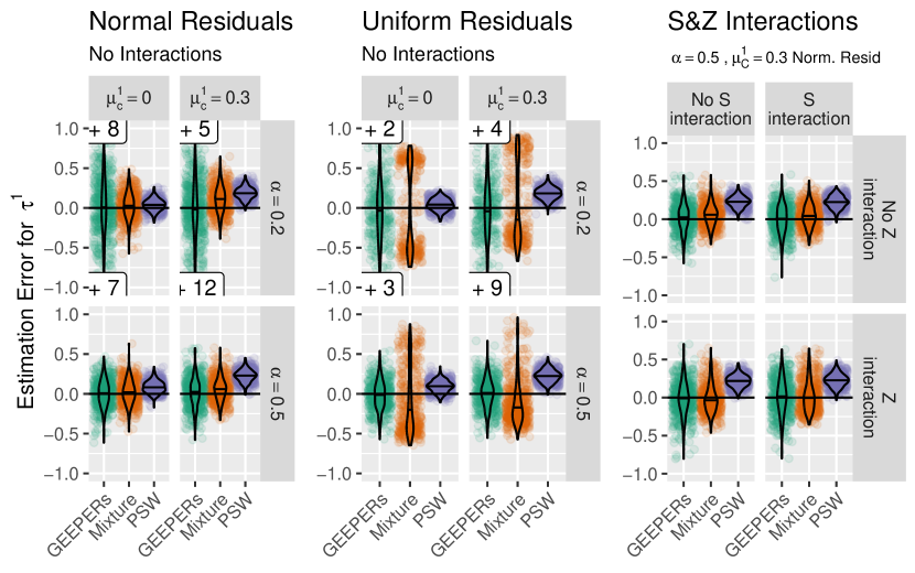
Figure 2: Violin and scatter plots of 500 simulation estimation errors for estimators described in Section 4.1.3 under varying conditions. For all plots, $n=500$; there were 500 replications for each set of conditions. Annotations indicate the number of extreme outliers excluded from the plotting area.

Figure 2 shows violin plots, layered on top of jittered scatter plots, showing estimation error for geepers, the mixture estimator, and the psw estimator of $\tau^{1}$ under various sets of conditions, and Table 2 shows empirical coverage of nominal 95% confidence interval estimates under a somewhat wider set of circumstances when $\mu_{C}^{1}=0.3$. More complete results, including root-mean-squared-error estimates, are in the online appendix. The leftmost panel of Figure 2 and the top line of Table 2 show results under conditions favorable to both the mixture model and to geepers—normal residuals and no interactions in the data generating model between covariates and either $S$ or $Z$. geepers was roughly unbiased, but less precise than the other two methods—when $\alpha=0.2$ it was much noisier, and when $\alpha=0.5$ it was only slightly less precise. The mixture estimator’s bias depended on $\mu_{C}^{1}$—when $\mu_{C}^{1}=0$, the bias was slight, and when $\mu_{C}^{1}=0.3$ the bias was more substantial. This is somewhat surprising, because when $\mu_{C}^{1}=0$, there was no separation between the principal strata in the control group, and previous literature (Griffin et al., 2008) has identified this scenario as a particular challenge for mixture modeling. The psw estimator was also biased—due, presumably, to the violation of Principal Ignorability, Assumption 4—inherent in the data generating model. On the other hand, the psw estimator had easily the lowest sampling variance of the three estimators. The middle panel of Figure 2 and the fifth line of Table 2 show a similar set of results for when the residuals in (18) are uniformly distributed. In this case, geepers and psw estimator, which do not assume normality, behaved in a similar fashion as in the normal case, but the mixture estimator showed a bimodal pattern–sometimes over-estimating $\tau^{1}$ and sometimes underestimating, but rarely estimating $\tau^{1}$ accurately. Credible intervals from the mixture model exhibited severe undercoverage, while geepers confidence intervals achieved at least their nominal level.

The rightmost panel of Figure 2 returns to the case of normal residuals—and only shows results when $\mu_{C}^{1}=0.3$ and $\alpha=0.5$—but introduces interactions in the data generating model between covariates and either $S_{T}$, $Z$, or both, violating Assumption 6. Fortunately, these interactions made little difference when $\alpha=0.5$; however, Table 2 shows that when $\alpha=0$ or 0.2, interactions between $\bm{X}$ and $Z$ were present (i.e. $\gamma_{3}\neq 0$) geepers 95% confidence intervals tended to under-cover. Nevertheless, coverage of geepers intervals was nearly always substantially higher than coverage of corresponding 95% credible intervals from mixture models.

Table 2: Empirical coverage of nominal 95% confidence intervals for estimates of $\tau^{1}$.

			$\alpha=0$		$\alpha=0.2$		$\alpha=0.5$
Residual Dist.	X:Z Int.?	X:S Int.?	geepers	Mixture	geepers	Mixture	geepers	Mixture
	No	No	0.99	0.99	0.97	0.97	0.96	0.96
	Yes	No	0.88	0.74	0.88	0.74	0.94	0.89
	No	Yes	1.00	1.00	0.98	0.97	0.97	0.96
Normal	Yes	Yes	0.90	0.77	0.90	0.77	0.94	0.88
	No	No	0.99	0.29	0.97	0.40	0.95	0.61
	Yes	No	0.83	0.11	0.87	0.20	0.93	0.48
	No	Yes	1.00	0.47	0.98	0.53	0.96	0.57
Uniform	Yes	Yes	0.83	0.15	0.88	0.21	0.94	0.53
Based on 500 replications. $n=500$, $\beta_{1}=0.3$. Simulation standard error $\approx 1$ percentage point.

5 Application: Estimating Treatment Effects for Implementation Subgroups

In a recent educational field experiment, middle school students completing their math schoolwork on a computer program were randomized between four conditions. These included two gamified programs—DragonBox and From Here to There (FH2T)—and two programs in which students used computers to work through a series of algebra problems taken from the district’s textbook—“Assistments” and an active control called “Business as Usual” (BAU). Students in ASSISTments had access to a series hints for each problem, culminating in a “bottom out” hint that contained the answer and were given immediate feedback on their answers. In the BAU condition students had no access to hints and received feedback only after completing the assignment. In all four conditions, students worked on their assigned math program in class on 12 different occasions spaced throughout the school year: a prior assessment, a mid-test, a post-test, and nine learning sessions. In this illustration, we will compare ASSISTments—the only condition featuring bottom-out hints—with each of the three others separately. Our goal is to estimate different treatment effects for groups of students who would, if assigned to ASSISTments, request few or many bottom out hints.

The literature on hints in online learning is mixed (see, e.g., Aleven et al., 2016; Goldin et al., 2012; Sales and Pane, 2021) in particular when it comes to requesting a bottom-out hint (called “bottoming out”). On the one hand, hints that include the correct answer are essentially worked examples, which can be beneficial to learning (Sweller and Cooper, 1985, e.g.). On the other hand, they allow students to “game the system,” by simply requesting enough hints to see the right answer, and use the software without ever working to solve any problems (e.g. Guo et al., 2008).

In this experiment, the ability to bottom out was only one of several differences between the treatment conditions. One way to disentangle the role of bottoming out in any treatment effect would be to estimate average treatment effects of being assigned to ASSISTments, relative to any of the other three, separately for subjects who would (if assigned to ASSISTments) bottom out frequently, and for subjects who would not. If the availability of bottom-out hints plays an important positive role in ASSISTments’ efficacy, we might expect larger effects of condition on students who would bottom out frequently than for those who would not; if bottom-out hints are harmful, we might expect the opposite. (These hypothetical results may be masked by other treatment effect heterogeneity between students who would or wouldn’t bottom out, but the results could still be informative.)

We gathered dichotomized data on whether students in ASSISTments requested more than the median number of bottom-out hints (i.e. 11). That is, $S_{T}=1$ for students who, if assigned to ASSISTments, would request at more than 11 bottom-out hints (“bottom-outers”), and $S_{T}=0$ for students who would request 11 or fewer (“non-bottom-outers”). The outcome of interest $Y$ in our example is students’ total scores on a ten-item posttest completed within the online tutoring system; $Y$ is an integer ranging from 0 to 10. The goal of our analysis will be to determine the principal effects $\tau_{1}=\mathbb{E}[Y_{T}-Y_{C}|S_{T}=0]$ and $\tau_{0}=\mathbb{E}[Y_{T}-Y_{C}|S_{T}=0]$, the average effects of assignment to ASSISTments (“$T$” subscripts) versus the other conditions (“$C$”) for bottom-outers and non-bottom-outers.

We also had access to data on a number of baseline covariates, including prior achievement, demographics, baseline measurements of student attitudes towards math and an indicator for whether students began the school year in remote or in-person instruction. Students with missing pretest scores were dropped from the analysis; missing data in other covariates was imputed with a Random Forest algorithm (Stekhoven and Buehlmann, 2012). Summary statistics are displayed in the online appendix.

The data analysis we present here is intended as a demonstration of geepers, rather than for its substantive conclusions, and our description omits discussion of some important methodological considerations, including attrition and post-selection inference. For a more complete discussion of the experimental design, the conditions being compared, and the impact analysis, please see Decker-Woodrow et al. (Forthcoming).

Due to privacy regulations, the data are not publicly available; however, interested analysts may access anonymized data by emailing the study’s principal investigator at erottmar@wpi.edu and signing a privacy agreement. Replication code for the analysis is available at https://github.com/adamSales/psGee.

We estimated principal scores using logistic regression of observed $S$ on school fixed effects and a set of baseline variables chosen with a combination of expert judgement and backwards selection based on the AIC, and evaluated model fit with binned residual plots (Gelman and Hill, 2006). The model was fit to data from students in the ASSISTments group, for whom bottom-out status ($S$) was observed; hence, the same model fit was used for all three treatment contrasts. The model was fairly successful in distinguishing bottom-outers from non-bottom-outers—the AUC, evaluated using out-of-sample predictions in a 10-fold cross-validation, was roughly 0.795. That is, in roughly 80% of bottom-outer/non-bottom-outer pairs of subjects, the bottom-outer will have a higher predicted probability from the model. Coefficient estimates are displayed in the online appendix.

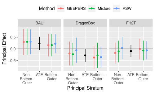
Figure 3: Principal Effects

Figure 3 shows principal effect estimates from geepers compared to analogous estimates using Bayesian mixture modeling and psw, alongside estimates of the overall average treatment effects, labeled “ATE.”. Outcome regressions in geepers and the mixture model included all of the covariates that were in the principal score model, in addition to students’ pretest scores; also, the models substituted class fixed effects for school fixed effects. Coefficient estimates are displayed in the online appendix.

The Bayesian mixture model assumed that outcomes were normally distributed, conditional on covariates and principal stratum, with a residual standard deviation that varied between principal strata. This modeling assumption is necessarily false, since post-test scores were integers between 0 and 10. All model parameters with support in $\mathbb{R}$ were given standard normal priors, while standard deviation parameters were given half-standard normal priors. The principal score and outcome models were fit simultaneously using a Markov Chain Monte Carlo algorithm (Stan Development Team, 2020).

The psw estimators did not include any covariate outcome modeling. Standard errors for the psw estimates were estimated using the bootstrap, with resampling done within schools.

For all three sets of estimators, approximate 95% confidence intervals were estimated by adding and subtracting twice the standard error from the point estimate (or twice the posterior standard deviation from the posterior mean, in the Bayesian mixture model).

The geepers results suggest little difference, if any, between the effects in the two principal strata. Estimated effects compared to BAU or DragonBox were slightly lower for bottom-outers than for non-bottom-outers, and estimated effects compared to FH2T were higher for non-bottom-outers. However, none of these differences is statistically significant, so opposite patterns, or no difference between principal effects at all, would also be consistent with the data. In fact, 95% confidence intervals for all principal effects include both positive and negative principal effects.

The other estimation strategies largely agreed with geepers, and with each other. This may suggest that the estimators’ various assumptions—additivity of treatment assignment effect for geepers and the mixture model, normal residuals for the mixture model, and principal ignorability for psw—were all innocuous and may have held approximately. Alternatively, violations of the different assumptions may have led to similar errors.

6 Discussion

geepers is a straightforward approach to principal effect estimation under strong monotonicity, built on widely-used regression models, which is more robust—though sometimes less precise—than alternative approaches under a wide array of scenarios.

There is good reason to hope that extensions to geepers, including cases in which $S$ takes more than two values, may be straightforward. For instance, in truncation by death problems (e.g. Zhang and Rubin, 2003; Ding et al., 2011) with weak monotonicity, $S_{i}=1$ if participant $i$ survives (or, more generally, if the outcome $Y_{i}$ is measured) and 0 otherwise, interest is typically in the principal effect for the “always survive” principal stratum in which $S_{Ti}=S_{ci}=1$. If, say, $S_{Ti}\geq S_{Ci}$, then every subject in the control condition with $S_{i}=1$ is in the always survive stratum, while those subjects in the treatment condition with $S_{i}=1$ are a mixture of the always survive and $S_{Ti}=1;\;S_{Ci}=0$ stratum. This scenario is broadly similar to the strong monotonicity, one-way noncompliance situation that this paper discussed. On the other hand, when no monotonicity assumption holds, both $S_{T}$ and $S_{C}$ will have to be imputed for every subject; further research is necessary to determine the appropriate way to do so.

Another direction of extension involved the principal score model (3). The performance of geepers in the simulation study of Section 4 depended heavily on the factor $\alpha$, which controlled the extent to which covariates could predict $S$. That suggests that when covariates are high-dimensional, geepers’ performance in applications could be optimized with a high-dimensional semi- or non-parametric model. If so, several further questions emerge. First, can the parameter $\alpha$ be extended to a more general parameter measuring the prediction accuracy of a non-parametric model. Second, if the principal score model cannot be formulated as the solution to a set of estimating equations, how should the standard error be computed? Lastly, can over-fit principal score models cause bias or other estimation problems, and if so, are there ways to protect against overfitting?

geepers is a flexible, easily-implementable method for principal effect estimation for one-way noncompliance, with predictive covariates; extensions to a broader set of circumstances could be a boon to causal modeling.

Online Appendices for “GEEPERs: Principal Stratification using Principal Scores and Stacked Estimating Equations”

Appendix A Proofs and Calculations

A.1 Proof for Lemma 1

As a preliminary, note that

$$\mathbb{E}[Y_{C}|e(\bm{X}^{S})] =\mathbb{E}\left\{\mathbb{E}[Y_{C}|e(\bm{X}^{S}),S_{T}]|e(\bm{X}^{S})\right\}$$

$$=\mathbb{E}\left\{\mathbb{E}[Y_{C}|S_{T}]|e(\bm{X}^{S})\right\}$$ by (8)

$$=\mathbb{E}[\mu_{C}^{1}S_{T}+\mu_{C}^{0}(1-S_{T})|e(\bm{X}^{S})]$$

$$=\mu_{C}^{1}e(\bm{X}^{S})+\mu_{C}^{0}(1-e(\bm{X}^{S}))$$

Then we have

$$\begin{split}\mathbb{E}[Y_{C}]=&\mathbb{E}\mathbb{E}[Y_{C}|e(\bm{X}^{S})]=\mu_{C}^{1}\mathbb{E}e(\bm{X}^{S})+\mu_{C}^{0}(1-\mathbb{E}e(\bm{X}^{S}))\\ =&\mu_{C}^{0}+\mathbb{E}e(\bm{X}^{S})(\mu_{C}^{1}-\mu_{C}^{0})\end{split}$$

Next we have

$$\mathbb{E}[Y_{C}e(\bm{X}^{S})] =\mathbb{E}\left\{\mathbb{E}[Y_{C}e(\bm{X}^{S})|e(\bm{X}^{S})]\right\}$$

$$=\mathbb{E}\left\{e(\bm{X}^{S})\mathbb{E}[Y_{C}|e(\bm{X}^{S})]\right\}$$

$$=\mathbb{E}\left\{e(\bm{X}^{S})\left[\mu_{C}^{1}e(\bm{X}^{S})+\mu_{C}^{0}(1-e(\bm{X}^{S}))\right]\right\}$$

$$=\mathbb{E}[e(\bm{X}^{S})]\mu_{C}^{0}+\mathbb{E}[e(\bm{X}^{S})^{2}](\mu_{C}^{1}-\mu_{C}^{0})$$

In the treatment group, $S_{T}$ is observed, so

$$\mathbb{E}[Y_{T}]= \mu_{T}^{0}+\mathbb{E}[S_{T}](\mu_{T}^{1}-\mu_{T}^{0})$$ and

$$\mathbb{E}[S_{T}Y_{T}]= \mathbb{E}[S_{T}]\mu_{T}^{0}+\mathbb{E}[S_{T}^{2}](\mu_{T}^{1}-\mu_{T}^{0})$$

Due to Assumption 2 (randomization), $\mathbb{E}[Y|Z=0]=\mathbb{E}[Y_{C}]$, $\mathbb{E}[Y|Z=1]=\mathbb{E}[Y_{T}]$, $\mathbb{E}[Ye(\bm{X}^{S})|Z=0]=\mathbb{E}[Y_{C}e(\bm{X}^{S})]$ and $\mathbb{E}[YS|Z=1]=\mathbb{E}[Y_{T}S_{T}]$, completing the proof.

A.2 Proof for Proposition 1

Replacing $S_{Ti}$ and $e(\bm{X}^{S})$ in (9) with $R_{i}$, as in (10), and replacing $\tilde{\Psi}_{i}$ with $\Psi_{i}=\begin{pmatrix}1&0&1&0\\ 0&1&0&1\\ 0&0&1&0\\ 0&0&0&1\end{pmatrix}\tilde{\Psi}_{i}$ gives an equivalent set of estimating equations $\sum_{i=1}^{n_{C}}\Psi_{i}=\bm{0}$ with $\Psi_{i}=$

$$\begin{pmatrix}Y_{i}-\mu_{C}^{0}-R_{i}(\mu_{C}^{1}-\mu_{C}^{0})-Z_{i}(\mu_{T}^{0}-\mu_{C}^{0})-Z_{i}R_{i}(\mu_{T}^{1}-\mu_{T}^{0}-\mu_{C}^{1}+\mu_{C}^{0})\\ R_{i}Y_{i}-R_{i}\mu_{C}^{0}-R_{i}^{2}(\mu_{C}^{1}-\mu_{C}^{0})-Z_{i}R_{i}(\mu_{T}^{0}-\mu_{C}^{0})-Z_{i}R_{i}^{2}(\mu_{T}^{0}-\mu_{T}^{1}-\mu_{C}^{0}+\mu_{C}^{1})\\ Z_{i}Y_{i}-Z_{i}\mu_{T}^{0}-Z_{i}R_{i}(\mu_{T}^{1}-\mu_{T}^{0})\\ Z_{i}R_{i}Y_{i}-Z_{i}R_{i}\mu_{T}^{0}-Z_{i}R_{i}^{2}(\mu_{T}^{1}-\mu_{T}^{0})\par\end{pmatrix}$$ (19)

These are equivalent to the estimating equations for OLS model (11) with $\beta_{0}=\mu_{C}^{0}$, $\beta_{1}=\mu_{C}^{1}-\mu_{C}^{0}$, $\beta_{2}=\mu_{T}^{0}-\mu_{C}^{0}$, and $\beta_{3}=\mu_{T}^{1}-\mu_{T}^{0}-\mu_{C}^{1}-\mu_{C}^{0}$. Therefore, under standard OLS regularity conditions the estimated parameter vector $\bm{\hat{\beta}}$ is consistent, completing the proof.

A.3 A Stronger Version of Proposition 2 and a Proof

Proposition 3

Say, for $i=1,\dots,n$, principal scores $e(\bm{X}^{S}_{i})$ are generated as (3), with parameters $\bm{\alpha}$ identified and estimable with M-estimation, and there exist $\beta_{0}$, $\beta_{1}$, $\beta_{2}$, $\beta_{3}$, $\bm{\gamma_{1}}$, $\bm{\gamma_{2}}$, $\bm{\gamma_{3}}$ amd $\bm{\gamma_{4}}$ such that

$$\begin{split}\mathbb{E}[Y_{i}|S_{T},Z,\bm{X}]=&\beta_{0}+\beta_{1}S_{Ti}+\beta_{2}Z_{i}+\beta_{3}Z_{i}S_{Ti}\\ &+\bm{\gamma_{1}}^{\prime}\bm{X}^{Y}_{i}+\bm{\gamma_{2}}^{\prime}\bm{X}^{Y}_{i}S_{Ti}+\bm{\gamma_{3}}^{\prime}\bm{X}^{Y}Z_{i}+\bm{\gamma_{4}}^{\prime}\bm{X}^{Y}_{i}Z_{i}S_{Ti}\end{split}$$ (20)

Then, under Assumptions 1, 2, and 3, if $e(\bm{X}^{S}_{i})$ is linearly independent of $\bm{X}^{Y}$, a researcher may follow the following procedure to estimate principal effects:

1. Estimate principal scores by fitting model (3) to data from the treatment group

2. Replace $S_{Ti}$ with $R_{i}$ (as defined in 10) in model (20) and fit with OLS

3. Estimate principal effects as:

   $$\begin{split}\hat{\tau}^{0}_{int}&\equiv\hat{\beta}_{2}+\bm{\hat{\gamma}_{3}}^{\prime}\overline{\bm{X}^{Y}}_{Z=1,S=0}\\ \hat{\tau}^{1}_{int}&\equiv\hat{\beta}_{2}+\hat{\beta}_{3}+(\bm{\hat{\gamma}_{3}}+\bm{\hat{\gamma}_{4}})^{\prime}\overline{\bm{X}^{Y}}_{Z=1,S=1}\end{split}$$ (21)

   where $\overline{\bm{X}^{Y}}_{Z=1,S=0}$ and $\overline{\bm{X}^{Y}}_{Z=1,S=0}$ are the vector of covariate sample means for the subsets of subjects with $Z=1$ and $S=0$ or $S=1$, respectively.

Then $\hat{\tau}^{0}_{G}$ and $\hat{\tau}^{1}_{int}$ are M-estimators, with $\hat{\tau}^{0}_{int}\rightarrow_{p}\tau^{0}$ and $\hat{\tau}^{1}_{G}\rightarrow_{p}\tau^{1}$ as $n\rightarrow\infty$. Under suitible regularity conditions, they are jointly asymptotically normal, with a variance of the form (14).

Equation (20) implies Assumption 6 with $\bm{\gamma_{2}}=\bm{\gamma_{3}}=\bm{\gamma_{4}}=0$.

Proof A.1.

First of all, by (20),

$$\begin{split}\mathbb{E}[Y_{T}-Y_{C}|S_{T}=0]&\\ =&\mathbb{E}[Y|Z=1,S_{T}=0]-\mathbb{E}[Y|Z=1,S_{T}=0]\\ =&\beta_{2}+\bm{\gamma_{3}}^{\prime}\mathbb{E}[\bm{X}^{Y}|S_{T}=0]\end{split}$$

and

$$\begin{split}\mathbb{E}[Y_{T}-Y_{C}|S_{T}=1]&\\ =&\mathbb{E}[Y|Z=1,S_{T}=1]-\mathbb{E}[Y|Z=1,S_{T}=1]\\ =&\beta_{2}+\beta_{3}+(\bm{\gamma_{3}}^{\prime}+\bm{\gamma_{4}}^{\prime})\mathbb{E}[\bm{X}^{Y}|S_{T}=1]\end{split}$$

Furthermore, $\overline{\bm{X}^{Y}}_{Z=1,S=0}\rightarrow\mathbb{E}[\bm{X}^{Y}|S_{T}=0]$ and $\overline{\bm{X}^{Y}}_{Z=1,S=1}\rightarrow\mathbb{E}[\bm{X}^{Y}|S_{T}=1]$ as $n\rightarrow\infty$.

We will show that the estimated coefficients from model (20), but with $R$ replacing $S_{T}$, fit with OLS, are consistent for $\bm{\beta}$ and $\bm{\gamma}$ from (20).

First, note that $\mathbb{E}[S]=\mathbb{E}\mathbb{E}[S|\bm{X}]=\mathbb{E}[e(\bm{X}^{S})]$ and

$$\mathbb{E}[\bm{X}S] =\mathbb{E}[\bm{X}S|Z=1]=\mathbb{E}[\bm{X}S|Z=0]\mbox{ (due to randomization)}$$

$$=\mathbb{E}[\bm{X}\mathbb{E}[S|\bm{X}]|Z=0]=\mathbb{E}[\bm{X}e(\bm{X}^{S})|Z=0]=\mathbb{E}[\bm{X}e(\bm{X}^{S})]$$

implying that, according to (20),

$$\begin{split}\mathbb{E}[Y|\bm{X},Z=0]&=\beta_{0}+\beta_{1}e(\bm{X}^{S})+\bm{\gamma_{1}}^{\prime}\bm{X^{Y}}+\bm{\gamma_{2}}^{\prime}\bm{X^{Y}}e(\bm{X}^{S})\\ &=\beta_{0}+\beta_{1}R+\bm{\gamma_{1}}^{\prime}\bm{X^{Y}}+\bm{\gamma_{2}}^{\prime}\bm{X^{Y}}R\\ \mathbb{E}[Y|\bm{X},S,Z=1]&=\beta_{0}+\beta_{2}+(\beta_{1}+\beta_{3})S+(\bm{\gamma_{1}}+\bm{\gamma_{3}})\bm{X}^{Y}+(\bm{\gamma_{2}}+\bm{\gamma_{4}})\bm{X}^{Y}S\\ &=\beta_{0}+\beta_{2}+(\beta_{1}+\beta_{3})R+(\bm{\gamma_{1}}+\bm{\gamma_{3}})\bm{X}^{Y}+(\bm{\gamma_{2}}+\bm{\gamma_{4}})\bm{X}^{Y}R\end{split}$$

Therefore,

$$\mathbb{E}[Y]= \mathbb{E}[Y|Z=0]+\mathbb{E}[Z]\left\{\mathbb{E}[Y|Z=1]-\mathbb{E}[Y|Z=0]\right\}$$

$$= \beta_{0}+\beta_{1}\mathbb{E}[R]+\beta_{2}\mathbb{E}[Z]+\beta_{3}\mathbb{E}[ZR]+\bm{\gamma_{1}}^{\prime}\mathbb{E}[\bm{X}^{Y}]+\bm{\gamma_{2}}^{\prime}\mathbb{E}[\bm{X}^{Y}R]$$

$$+\bm{\gamma_{3}}^{\prime}\mathbb{E}[\bm{X}^{Y}Z]+\bm{\gamma_{4}}\mathbb{E}[\bm{X}^{Y}RZ]$$

Analogous reasoning leads to expressions for $\mathbb{E}[RY]$, $\mathbb{E}[\bm{X}^{Y}Y]$, $\mathbb{E}[ZY]$, $\mathbb{E}[ZRY]$, $\mathbb{E}[\bm{X}^{Y}YZ]$, and $\mathbb{E}[\bm{X}^{Y}RZY]$. These, in turn, give rise to estimating equations

$$\begin{split}&\psi_{i}=\\ &\begin{pmatrix}Y_{i}\\ \phantom{}\\ Y_{i}R_{i}\\ \phantom{}\\ Y_{i}Z_{i}\\ \phantom{}\\ Y_{i}Z_{i}R_{i}\\ \phantom{}\\ Y_{i}\bm{X}^{Y}_{i}\\ \phantom{}\\ Y_{i}\bm{X}^{Y}_{i}R_{i}\\ \phantom{}\\ Y_{i}\bm{X}^{Y}_{i}Z_{i}\\ \phantom{}\\ Y_{i}\bm{X}^{Y}_{i}Z_{i}R_{i}\\ \phantom{}\end{pmatrix}-\begin{pmatrix}[l]\beta_{0}+\beta_{1}R_{i}+\beta_{2}Z_{i}+\beta_{3}Z_{i}R_{i}\\ \quad+\left\{\bm{\gamma_{1}}^{\prime}+R_{i}\bm{\gamma_{2}}^{\prime}+Z_{i}\bm{\gamma_{3}}^{\prime}+R_{i}Z_{i}\bm{\gamma_{4}}^{\prime}\right\}\bm{X}^{Y}\\ \beta_{0}R_{i}+\beta_{1}R_{i}^{2}+\beta_{2}Z_{i}R_{i}+\beta_{3}Z_{i}R_{i}^{2}\\ \quad+R_{i}\left\{\bm{\gamma_{1}}^{\prime}+R_{i}\bm{\gamma_{2}}^{\prime}+Z_{i}\bm{\gamma_{3}}^{\prime}+R_{i}Z_{i}\bm{\gamma_{4}}^{\prime}\right\}\bm{X}^{Y}\\ (\beta_{0}+\beta_{2})Z_{i}+(\beta_{1}+\beta_{3})R_{i}Z_{i}\\ \quad+Z_{i}\left\{\bm{\gamma_{1}}^{\prime}+R_{i}\bm{\gamma_{2}}^{\prime}+Z_{i}\bm{\gamma_{3}}^{\prime}+R_{i}Z_{i}\bm{\gamma_{4}}^{\prime}\right\}\bm{X}^{Y}\\ \beta_{0}Z_{i}R_{i}+(\beta_{1}+\beta_{3})Z_{i}R_{i}^{2}+\beta_{2}Z_{i}R_{i}\\ \quad+Z_{i}R_{i}\left\{\bm{\gamma_{1}}^{\prime}+\bm{\gamma_{3}}^{\prime}+R_{i}(\bm{\gamma_{2}}^{\prime}+\bm{\gamma_{4}}^{\prime})\right\}\bm{X}^{Y}\\ \beta_{0}\bm{X}^{Y\prime}+\beta_{1}R_{i}\bm{X}^{Y\prime}+\beta_{2}Z_{i}\bm{X}^{Y\prime}+\beta_{3}Z_{i}R_{i}\bm{X}^{Y\prime}\\ \quad{}+\left\{\bm{\gamma_{1}}^{\prime}+R_{i}\bm{\gamma_{2}}^{\prime}+Z_{i}\bm{\gamma_{3}}^{\prime}+R_{i}Z_{i}\bm{\gamma_{4}}^{\prime}\right\}\bm{X}^{Y}\bm{X}^{Y\prime}\\ \beta_{0}R_{i}\bm{X}^{Y\prime}+\beta_{1}R_{i}^{2}\bm{X}^{Y\prime}+\beta_{2}Z_{i}R_{i}\bm{X}^{Y\prime}+\beta_{3}Z_{i}R_{i}^{2}\bm{X}^{Y\prime}\\ \quad{}+R_{i}\left\{\bm{\gamma_{1}}^{\prime}+R_{i}\bm{\gamma_{2}}^{\prime}+Z_{i}\bm{\gamma_{3}}^{\prime}+R_{i}Z_{i}\bm{\gamma_{4}}^{\prime}\right\}\bm{X}^{Y}\bm{X}^{Y\prime}\\ (\beta_{0}+\beta_{2})Z_{i}\bm{X}^{Y\prime}+(\beta_{1}+\beta_{3})R_{i}Z_{i}\bm{X}^{Y\prime}\\ \quad{}+Z_{i}\left\{\bm{\gamma_{1}}^{\prime}+R_{i}\bm{\gamma_{2}}^{\prime}+Z_{i}\bm{\gamma_{3}}^{\prime}+R_{i}Z_{i}\bm{\gamma_{4}}^{\prime}\right\}\bm{X}^{Y}\bm{X}^{Y\prime}\\ \beta_{0}R_{i}Z_{i}\bm{X}^{Y\prime}+\beta_{1}R_{i}^{2}Z_{i}\bm{X}^{Y\prime}+\beta_{2}R_{i}Z_{i}\bm{X}^{Y\prime}+\beta_{3}Z_{i}R_{i}^{2}\bm{X}^{Y\prime}\\ \quad{}+R_{i}Z_{i}\left\{\bm{\gamma_{1}}^{\prime}+R_{i}\bm{\gamma_{2}}^{\prime}+Z_{i}\bm{\gamma_{3}}^{\prime}+R_{i}Z_{i}\bm{\gamma_{4}}^{\prime}\right\}\bm{X}^{Y}\bm{X}^{Y\prime}\\ \end{pmatrix}\end{split}$$

with $\mathbb{E}[\psi_{i}]=0$. These are the estimating equations for the regression model (20), with $R$ replacing $S_{T}$, fit by OLS. Under standard OLS regularity conditions, the estimated coefficients of that model are consistent, completing the proof.

A.4 Sandwich Matrix Calculations

Here we will derive the sandwich variance-covariance matrix for the geepers estimate without interactions between $\bm{X}$ and either $Z$ or $S_{T}$—i.e. with $\bm{\gamma_{2}}=\bm{\gamma_{3}}=\bm{\gamma_{4}}=0$ in the notation of (20)—and estimating principal scores using a generalized linear model.

We propose estimating principal effects in two stages. First, fit the model

$$e(\bm{X}^{S}_{i})=Pr(S_{Ti}=1|\bm{X}^{S}_{i})=f(\bm{\alpha}^{\prime}\bm{\tilde{X}^{S}}_{i})$$ (22)

for some inverse link function $f(\cdot)$, where $\bm{\tilde{X}^{S}}_{i}=[1,\bm{X}^{S}_{i}]$, using (observed) values from the treatment group, and estimating $\hat{\alpha}$. Then let

$$\hat{p}_{i}=f(\bm{\hat{\alpha}}^{\prime}\bm{\tilde{X}^{S}}_{i})$$ (23)

for all subjects in the experiment.

Finally, fit model

$$Y_{i}=\beta_{0}+\beta_{1}r_{i}+\beta_{2}Z_{i}+\beta_{3}Z_{i}R_{i}+\bm{\gamma}^{\prime}\bm{X}^{Y}_{i}+\epsilon_{i}$$ (24)

to estimate $\bm{\beta}$ and hence principal effects, where $\bm{x}_{i}$ is a set of covariates predictive of $Y$ within principal strata. Let $\bm{\beta}=[\beta_{0},\beta_{1},\beta_{2},\beta_{3},\bm{\gamma}^{\prime}]^{\prime}$.

Following (13), let $\bm{\Lambda}(Z_{i},S_{i},\bm{X}^{S}_{i},\bm{X}^{Y}_{i},Y_{i};\bm{\alpha},\bm{\beta})=\begin{pmatrix}Z_{i}\Omega(\bm{X}^{S}_{i},S_{i};\bm{\alpha})\\ \Psi(\bm{X}^{Y}_{i},\bm{X}^{S}_{i},Y_{i},Z_{i},R_{i}(\bm{\alpha});\bm{\beta})\end{pmatrix}$, the stacked estimating equations of (22) and (24). Going forward, for the sake of brevety, we will write $\bm{\Lambda}_{i}(\bm{\alpha},\bm{\beta})=\bm{\Lambda}(Z_{i},S_{i},\bm{X}^{S}_{i},\bm{X}^{Y}_{i},Y_{i};\bm{\hat{\alpha}},\bm{\hat{\beta}})$, where dependence on the data for $i$ is captured in the subscript $i$, with similar meanings for $\Psi_{i}(\bm{\alpha},\bm{\beta})$ and $\omega_{i}(\bm{\alpha})$.

The variance-covariance matrix for $\bm{\hat{\alpha}}$ and $\bm{\hat{\beta}}$ can be estimated as:

$$\widehat{var}\left([\bm{\hat{\alpha}}^{\prime},\bm{\hat{\beta}}^{\prime}]^{\prime}\right)=A^{-1}BA^{-t}$$

where

$$A=\sum_{i}\frac{\partial}{\partial[\bm{\alpha},\bm{\beta}]^{\prime}}\bm{\Lambda}_{i}\Bigr{|}_{\begin{subarray}{c}\bm{\alpha}=\bm{\hat{\alpha}}\\ \bm{\beta}=\bm{\hat{\beta}}\end{subarray}}$$

and

$$B=\sum_{i}\bm{\Lambda}_{i}(\bm{\hat{\alpha}},\bm{\hat{\beta}})\bm{\Lambda}_{i}(\bm{\hat{\alpha}},\bm{\hat{\beta}})^{\prime}$$

Following Carroll et al. [2006, p. 373], we can decompose the matrices into diagonal elements

$$\begin{split}A_{1,1}&=\sum_{i}\partial\Omega_{i}/\partial\bm{\alpha}|_{\bm{\alpha}=\bm{\hat{\alpha}}}\\ A_{2,2}&=\sum_{i}\partial\Psi_{i}/\partial\bm{\beta}|_{\bm{\beta}=\bm{\hat{\beta}}}\\ B_{1,1}&=\sum_{i}\Omega_{i}(\bm{\hat{\alpha}})\Omega_{i}(\bm{\hat{\alpha}})^{\prime}\\ B_{2,2}&=\sum_{i}\Psi_{i}(\bm{\hat{\alpha}},\bm{\hat{\beta}})\Psi_{i}(\bm{\hat{\alpha}},\bm{\hat{\beta}})^{\prime}\end{split}$$

that pertain to the parameter sets $\bm{\alpha}$ and $\bm{\beta}$ and the estimating equations for models (22) and (24), respectively, and

$$\begin{split}A_{21}&=\sum_{i}\partial\Psi_{i}/\partial\bm{\alpha}|_{\bm{\alpha}=\bm{\hat{\alpha}}}\\ B_{12}=B_{21}^{\prime}&=\sum_{i}\Omega_{i}(\bm{\hat{\alpha}})\Psi_{i}(\bm{\hat{\alpha}},\bm{\hat{\beta}})^{\prime}\end{split}$$

which capture to the dependence of model (24) on the parameters $\bm{\alpha}$ from (22) and the covariance between the estimating equations of the two models. The sub-matrix $A_{12}=\sum_{i}\partial\Omega_{i}/\partial\bm{\beta}=0$, since (22) does not depend on $\bm{\beta}$.

The diagonal matrices $A_{1,1}$ and $A_{2,2}$ and $B_{1,1}$ and $B_{2,2}$ are all the typical “bread” and “meat” matrices from M-estimation of generalized linear models and OLS. Calculation of the matrices $B_{12}$ and $B_{21}$ is straightforward after vectors $\Omega_{i}(\bm{\hat{\alpha}})$ and $\Psi_{i}(\bm{\hat{\alpha}},\bm{\hat{\beta}})$ have been calculated. Some specialized calculation is necessary for matrix $A_{21}$.

A.5 $A_{21}$ Matrix

The estimating equations for the regression (24) are

$$\psi(Y_{i},\bm{X}^{Y}_{i},\bm{X}^{S}_{i},\bm{\beta},\alpha)=X_{i}Y_{i}-X_{i}X_{i}^{\prime}\bm{\beta}$$ (25)

Where $X_{i}=[1,r_{i},Z_{i},r_{i}Z_{i},\bm{X}^{Y\prime}_{i}]^{\prime}$. In other words,

$$\psi(Y_{i}, \bm{X}^{Y}_{i},\bm{X}^{S}_{i},\bm{\beta},\bm{\alpha})=$$

$$\left\{\begin{array}[]{l}Y_{i}-\left(\beta_{0}+\beta_{1}r_{i}+\beta_{2}Z_{i}+\beta_{3}Z_{i}r_{i}+\bm{\gamma}^{\prime}\bm{X}^{Y}_{i}\right)\\ r_{i}Y_{i}-r_{i}\left(\beta_{0}+\beta_{2}Z_{i}+\bm{\gamma}^{\prime}\bm{X}^{Y}_{i}\right)-r_{i}^{2}\left(\beta_{1}+\beta_{3}Z_{i}\right)\\ Z_{i}Y_{i}-Z_{i}\left(\beta_{0}+\beta_{1}r_{i}+\beta_{2}Z_{i}+\beta_{3}Z_{i}r_{i}+\bm{\gamma}^{\prime}\bm{X}^{Y}_{i}\right)\\ Z_{i}r_{i}Y_{i}-Z_{i}r_{i}\left(\beta_{0}+\beta_{2}Z_{i}+\bm{\gamma}^{\prime}\bm{X}^{Y}_{i}\right)-Z_{i}r_{i}^{2}\left(\beta_{1}+\beta_{3}Z_{i}\right)\\ \bm{X}^{Y}_{i}Y_{i}-\bm{X}^{Y}_{i}\left(\beta_{0}+\beta_{1}r_{i}+\beta_{2}Z_{i}+\beta_{3}Z_{i}r_{i}+\bm{\gamma}^{\prime}\bm{X}^{Y}_{i}\right)\end{array}\right\}$$

(noting that $Z^{2}=Z$). These depend on $\bm{\alpha}$ when $r_{i}=p_{i}$, i.e. when $Z_{i}=0$.Then note that, following (23), and letting $\eta_{i}=\bm{\alpha}^{\prime}\bm{\tilde{X}^{S}}_{i}$

$$\frac{\partial p_{i}}{\partial\bm{\alpha}^{\prime}}=f^{\prime}(\eta_{i})\frac{\partial\eta_{i}}{\partial\bm{\alpha}^{\prime}}=f^{\prime}(\eta_{i})\bm{\tilde{X}^{S\prime}}_{i}$$ (26)

and that

$$\frac{\partial p_{i}^{2}}{\partial\bm{\alpha}^{\prime}}=2p_{i}\frac{\partial p_{i}}{\partial\bm{\alpha}^{\prime}}=2f(\eta)f^{\prime}(\eta_{i})\bm{\tilde{X}^{S\prime}}_{i}=2p_{i}f^{\prime}(\eta_{i})\bm{\tilde{X}^{S\prime}}_{i}$$ (27)

Then if $r_{i}=p_{i}$,

$$\frac{\partial}{\partial\bm{\alpha}^{\prime}} \psi(Y_{i},\bm{X}^{Y}_{i},\bm{\beta},\bm{\alpha})=$$

$$\left[\begin{array}[]{c}-(\beta_{1})f^{\prime}(\eta_{i})\bm{\tilde{X}^{S\prime}}_{i}\\ \left[Y_{i}-X_{i}^{\prime}\bm{\beta}-2p_{i}(\beta_{1})\right]f^{\prime}(\eta_{i})\bm{\tilde{X}^{S\prime}}_{i}\\ 0\\ 0\\ -\beta_{1}f^{\prime}(\eta_{i})\bm{X}^{Y}_{i}\bm{\tilde{X}^{S\prime}}_{i}\end{array}\right]$$

If $r_{i}=S_{i}$, $\frac{\partial}{\partial\bm{\alpha}^{\prime}}\psi(Y_{i},\bm{X}^{Y}_{i},\bm{\beta},\bm{\alpha})=0$.

Appendix B Simulation Results

B.1 Plot of AUC versus $\alpha$

B.2 Full Empirical 95% Interval Coverage Results

					$\alpha=0$		$\alpha=0.2$		$\alpha=0.5$
Res. Dist.	X:Z Int.?	X:S Int.?	$\beta_{1}$	Prin. Eff	GEEPERs	Mixture	GEEPERs	Mixture	GEEPERs	Mixture
	No	No	0.0	$\tau^{0}$	1.00	1.00	0.98	0.98	0.97	0.96
	No	No	0.0	$\tau^{1}$	1.00	1.00	0.97	0.97	0.97	0.95
	Yes	No	0.0	$\tau^{0}$	0.84	0.70	0.91	0.74	0.93	0.81
	Yes	No	0.0	$\tau^{1}$	0.85	0.70	0.91	0.74	0.93	0.82
	No	Yes	0.0	$\tau^{0}$	1.00	1.00	0.98	0.99	0.95	0.95
	No	Yes	0.0	$\tau^{1}$	1.00	0.99	0.98	0.99	0.95	0.95
	Yes	Yes	0.0	$\tau^{0}$	0.88	0.76	0.91	0.77	0.94	0.83
Norm	Yes	Yes	0.0	$\tau^{1}$	0.86	0.74	0.92	0.76	0.94	0.82
	No	No	0.0	$\tau^{0}$	1.00	0.15	0.96	0.24	0.96	0.50
	No	No	0.0	$\tau^{1}$	1.00	0.16	0.97	0.23	0.95	0.49
	Yes	No	0.0	$\tau^{0}$	0.85	0.05	0.83	0.09	0.95	0.34
	Yes	No	0.0	$\tau^{1}$	0.85	0.06	0.85	0.09	0.93	0.33
	No	Yes	0.0	$\tau^{0}$	1.00	0.27	0.99	0.26	0.95	0.50
	No	Yes	0.0	$\tau^{1}$	1.00	0.28	0.98	0.26	0.96	0.52
	Yes	Yes	0.0	$\tau^{0}$	0.83	0.11	0.86	0.18	0.92	0.45
Unif	Yes	Yes	0.0	$\tau^{1}$	0.81	0.11	0.85	0.17	0.92	0.45
	No	No	0.3	$\tau^{0}$	0.99	0.99	0.97	0.98	0.95	0.96
	No	No	0.3	$\tau^{1}$	0.99	0.99	0.97	0.97	0.96	0.96
	Yes	No	0.3	$\tau^{0}$	0.88	0.75	0.88	0.76	0.94	0.89
	Yes	No	0.3	$\tau^{1}$	0.88	0.74	0.88	0.74	0.94	0.89
	No	Yes	0.3	$\tau^{0}$	0.99	0.99	0.97	0.96	0.96	0.97
	No	Yes	0.3	$\tau^{1}$	1.00	1.00	0.98	0.97	0.97	0.96
	Yes	Yes	0.3	$\tau^{0}$	0.90	0.78	0.90	0.76	0.93	0.89
Norm	Yes	Yes	0.3	$\tau^{1}$	0.90	0.77	0.90	0.77	0.94	0.88
	No	No	0.3	$\tau^{0}$	0.99	0.29	0.98	0.39	0.95	0.61
	No	No	0.3	$\tau^{1}$	0.99	0.29	0.97	0.40	0.95	0.61
	Yes	No	0.3	$\tau^{0}$	0.83	0.12	0.87	0.21	0.94	0.48
	Yes	No	0.3	$\tau^{1}$	0.83	0.11	0.87	0.20	0.93	0.48
	No	Yes	0.3	$\tau^{0}$	1.00	0.47	0.97	0.49	0.95	0.60
	No	Yes	0.3	$\tau^{1}$	1.00	0.47	0.98	0.53	0.96	0.57
	Yes	Yes	0.3	$\tau^{0}$	0.83	0.16	0.89	0.21	0.95	0.52
Unif	Yes	Yes	0.3	$\tau^{1}$	0.83	0.15	0.88	0.21	0.94	0.53

B.3 Full RMSE Results

					$\alpha=0.2$			$\alpha=0.5$
Residual Dist.	X:Z Int.?	X:S Int.?	$\beta_{1}$	Prin. Eff	GEEPERs	Mixture	PSW	GEEPERs	Mixture	PSW
	No	No	0.0	$\tau^{0}$	0.56	0.17	0.09	0.19	0.16	0.24
	No	No	0.0	$\tau^{1}$	0.57	0.17	0.08	0.19	0.16	0.24
	Yes	No	0.0	$\tau^{0}$	0.94	0.29	0.09	0.23	0.18	0.24
	Yes	No	0.0	$\tau^{1}$	0.94	0.30	0.09	0.23	0.18	0.23
	No	Yes	0.0	$\tau^{0}$	0.48	0.17	0.08	0.18	0.15	0.23
	No	Yes	0.0	$\tau^{1}$	0.46	0.16	0.08	0.19	0.15	0.24
	Yes	Yes	0.0	$\tau^{0}$	0.98	0.29	0.09	0.23	0.20	0.24
Normal	Yes	Yes	0.0	$\tau^{1}$	0.99	0.29	0.09	0.23	0.20	0.24
	No	No	0.0	$\tau^{0}$	0.42	0.55	0.08	0.18	0.31	0.24
	No	No	0.0	$\tau^{1}$	0.42	0.54	0.08	0.18	0.31	0.24
	Yes	No	0.0	$\tau^{0}$	1.58	0.58	0.09	0.22	0.34	0.24
	Yes	No	0.0	$\tau^{1}$	1.60	0.57	0.09	0.22	0.35	0.24
	No	Yes	0.0	$\tau^{0}$	0.41	0.53	0.09	0.19	0.30	0.24
	No	Yes	0.0	$\tau^{1}$	0.41	0.54	0.08	0.19	0.31	0.23
	Yes	Yes	0.0	$\tau^{0}$	2.70	0.55	0.09	0.22	0.35	0.24
Uniform	Yes	Yes	0.0	$\tau^{1}$	2.29	0.57	0.09	0.24	0.35	0.24
	No	No	0.3	$\tau^{0}$	0.52	0.20	0.20	0.13	0.11	0.23
	No	No	0.3	$\tau^{1}$	0.55	0.20	0.20	0.13	0.11	0.23
	Yes	No	0.3	$\tau^{0}$	1.03	0.34	0.20	0.16	0.15	0.23
	Yes	No	0.3	$\tau^{1}$	1.06	0.33	0.21	0.17	0.16	0.23
	No	Yes	0.3	$\tau^{0}$	0.52	0.22	0.20	0.13	0.11	0.23
	No	Yes	0.3	$\tau^{1}$	0.51	0.22	0.21	0.13	0.11	0.23
	Yes	Yes	0.3	$\tau^{0}$	1.79	0.32	0.20	0.16	0.16	0.23
Normal	Yes	Yes	0.3	$\tau^{1}$	1.81	0.33	0.20	0.17	0.16	0.23
	No	No	0.3	$\tau^{0}$	0.60	0.50	0.20	0.13	0.32	0.23
	No	No	0.3	$\tau^{1}$	0.60	0.50	0.20	0.13	0.33	0.23
	Yes	No	0.3	$\tau^{0}$	0.93	0.56	0.20	0.16	0.36	0.23
	Yes	No	0.3	$\tau^{1}$	0.91	0.57	0.20	0.17	0.36	0.24
	No	Yes	0.3	$\tau^{0}$	0.45	0.47	0.20	0.12	0.29	0.23
	No	Yes	0.3	$\tau^{1}$	0.45	0.46	0.20	0.12	0.29	0.24
	Yes	Yes	0.3	$\tau^{0}$	1.25	0.55	0.20	0.16	0.34	0.23
Uniform	Yes	Yes	0.3	$\tau^{1}$	1.28	0.56	0.20	0.17	0.34	0.23

Appendix C More Results from Application

C.1 Summary Statistics

	level	ASSISTments	BAU	Miss. %	Imp. Err.
Baseline
n		461	428
Pretest		-0.22 (2.63)	-0.37 (2.64)	0.0	0
Gr. 5 Stand. Test		578.16 (60.39)	580.87 (59.71)	11.5	1754.93
Gender (n (%))	Female	202 (49.3)	176 (46.2)	11.0
	Male	208 (50.7)	205 (53.8)
Race/Eth. (n (%))	White	100 (44.2)	73 (36.3)	52.0
	Asian	40 (17.7)	44 (21.9)
	Hispanic	42 (18.6)	32 (15.9)
	Other	44 (19.5)	52 (25.9)
Has EIP (n (%))		27 ( 6.6)	28 ( 7.4)	11.5	0.08
Has IEP (n (%))		39 ( 9.5)	33 ( 8.7)	11.0	0.1
ESOL (n (%))		23 ( 5.6)	33 ( 8.7)	11.0	0.04
Gifted (n (%))		71 (17.3)	73 (19.2)	11.0	0.16
log(Pretest ToT)		4.14 (0.71)	4.16 (0.81)	0.0	0
Math Anxiety		13.35 (5.77)	13.50 (5.70)	6.0	0.31
Math Neg. React.		3.06 (2.31)	3.13 (2.33)	6.0	1.29
Numerical Conf.		4.75 (2.67)	4.81 (2.70)	6.0	2.07
Post-Treatment
Posttest		4.44 (2.84)	4.37 (2.87)	32.6
Bottom Out (%)		222 (48.2)	0 ( 0.0)	0.0

C.2 Regression Results

Regression estimates from principal score logit model and three outcome regressions for geepers estimates. Standard errors shown are nominal regression errors, not sandwich corrected. Fixed-effect estimates for school (PS-model) or classroom (outcome models) are omitted.

	psModel	BAU	FH2T	DragonBox
(Intercept)	$-2.14$	$1.73$	$2.83^{***}$	$2.51^{**}$
	$(1.26)$	$(0.92)$	$(0.72)$	$(0.92)$
Scale.Score5	$-0.59^{**}$	$0.21$	$0.45^{***}$	$0.05$
	$(0.19)$	$(0.13)$	$(0.10)$	$(0.13)$
ESOL1	$-0.83$	$0.09$	$-0.46$	$-0.49$
	$(0.64)$	$(0.36)$	$(0.27)$	$(0.35)$
IEP1	$-1.34^{**}$	$0.15$	$0.23$	$0.10$
	$(0.46)$	$(0.29)$	$(0.25)$	$(0.28)$
pre.total_time_on_tasks	$-0.45^{**}$	$-0.13$	$0.08$	$-0.00$
	$(0.15)$	$(0.09)$	$(0.07)$	$(0.10)$
pre_MSE_total_score	$-0.18$	$0.20^{*}$	$0.12$	$0.35^{***}$
	$(0.13)$	$(0.08)$	$(0.07)$	$(0.08)$
fullYear5TRUE	$1.40^{*}$	$-0.13$	$-0.10$	$0.06$
	$(0.58)$	$(0.33)$	$(0.29)$	$(0.34)$
pre_MA_total_scoreNATRUE	$-3.20^{***}$
	$(0.71)$
GenderM	$0.17$	$-0.19$	$-0.34^{**}$	$-0.27$
	$(0.25)$	$(0.15)$	$(0.13)$	$(0.16)$
raceEthHispanic/Latino	$-0.56$	$0.28$	$0.33$	$0.23$
	$(0.46)$	$(0.29)$	$(0.21)$	$(0.28)$
raceEthAsian	$-0.43$	$0.66^{*}$	$0.62^{**}$	$0.82^{**}$
	$(0.42)$	$(0.28)$	$(0.22)$	$(0.30)$
raceEthOther	$-0.13$	$0.45$	$0.21$	$0.10$
	$(0.49)$	$(0.29)$	$(0.23)$	$(0.30)$
GIFTED1	$-0.24$	$0.66^{**}$	$0.43^{*}$	$0.34$
	$(0.37)$	$(0.24)$	$(0.19)$	$(0.26)$
pre_PS_tasks_total_score	$0.01$
	$(0.19)$
$\text{pre\_PS\_tasks\_total\_score}^{2}$	$-0.41^{**}$
	$(0.13)$
Z		$0.29$	$-0.17$	$-0.20$
		$(0.28)$	$(0.22)$	$(0.27)$
Sp		$0.03$	$-0.22$	$0.04$
		$(0.52)$	$(0.41)$	$(0.52)$
pre_PS_tasks_total_score		$0.34^{**}$	$0.37^{***}$	$0.23$
		$(0.12)$	$(0.09)$	$(0.12)$
pre.total_math_score		$0.14^{**}$	$0.24^{***}$	$0.15^{**}$
		$(0.05)$	$(0.04)$	$(0.05)$
pre.total_math_scoreNATRUE		$-0.35$	$0.18$	$-0.44$
		$(0.45)$	$(0.36)$	$(0.43)$
Z:Sp		$-0.14$	$0.17$	$-0.17$
		$(0.49)$	$(0.39)$	$(0.49)$
AIC	$447.55$
BIC	$539.47$
Log Likelihood	$-200.78$
Deviance	$401.55$
Num. obs.	$402$	$787$	$1193$	$771$
R2		$0.60$	$0.60$	$0.63$
Adj. R2		$0.52$	$0.55$	$0.54$
${}^{***}p<0.001$; ${}^{**}p<0.01$; ${}^{*}p<0.05$

References

- Aleven et al. [2016] Vincent Aleven, Ido Roll, Bruce M McLaren, and Kenneth R Koedinger. Help helps, but only so much: Research on help seeking with intelligent tutoring systems. International Journal of Artificial Intelligence in Education, 26(1):205–223, 2016.
- Angrist et al. [1996] Joshua D Angrist, Guido W Imbens, and Donald B Rubin. Identification of causal effects using instrumental variables. Journal of the American statistical Association, 91(434):444–455, 1996.
- Boos et al. [2013] Dennis D Boos, Leonard A Stefanski, et al. Essential statistical inference. Springer, 2013.
- Bradley [1997] Andrew P Bradley. The use of the area under the roc curve in the evaluation of machine learning algorithms. Pattern recognition, 30(7):1145–1159, 1997.
- Carroll et al. [2006] Raymond J Carroll, David Ruppert, Leonard A Stefanski, and Ciprian M Crainiceanu. Measurement error in nonlinear models: a modern perspective. Chapman and Hall/CRC, 2006.
- Decker-Woodrow et al. [Forthcoming] Lauren E Decker-Woodrow, Craig Mason, Jenny Chan, Ji-Eun Lee, Adam C Sales, Allison Liu, and Shihfen Tu. The impacts of three educational technologies on algebraic understanding in the context of covid-19. AERA Open, Forthcoming.
- Ding and Lu [2017] P. Ding and J. Lu. Principal stratification analysis using principal scores. Journal of the Royal Statistical Society: Series B (Statistical Methodology), 79:757–777, 2017.
- Ding et al. [2011] Peng Ding, Zhi Geng, Wei Yan, and Xiao-Hua Zhou. Identifiability and estimation of causal effects by principal stratification with outcomes truncated by death. Journal of the American Statistical Association, 106(496):1578–1591, 2011.
- Feller et al. [2017] Avi Feller, Fabrizia Mealli, and Luke Miratrix. Principal score methods: Assumptions, extensions, and practical considerations. Journal of Educational and Behavioral Statistics, 42(6):726–758, 2017.
- Frangakis and Rubin [2002] Constantine E Frangakis and Donald B Rubin. Principal stratification in causal inference. Biometrics, 58(1):21–29, 2002.
- Gelman and Hill [2006] Andrew Gelman and Jennifer Hill. Data analysis using regression and multilevel/hierarchical models. Cambridge university press, 2006.
- Goldin et al. [2012] Ilya M Goldin, Kenneth R Koedinger, and Vincent Aleven. Learner differences in hint processing. International Educational Data Mining Society, 2012.
- Griffin et al. [2008] Beth Ann Griffin, Daniel F McCaffery, and Andrew R Morral. An application of principal stratification to control for institutionalization at follow-up in studies of substance abuse treatment programs. The annals of applied statistics, 2(3):1034, 2008.
- Guo et al. [2008] Yu Guo, Joseph E Beck, and Neil T Heffernan. Trying to reduce bottom-out hinting: Will telling student how many hints they have left help? In International Conference on Intelligent Tutoring Systems, pages 774–778. Springer, 2008.
- Ho et al. [2022] Nhat Ho, Avi Feller, Evan Greif, Luke Miratrix, and Natesh Pillai. Weak separation in mixture models and implications for principal stratification. In Gustau Camps-Valls, Francisco J. R. Ruiz, and Isabel Valera, editors, Proceedings of The 25th International Conference on Artificial Intelligence and Statistics, volume 151 of Proceedings of Machine Learning Research, pages 5416–5458. PMLR, 28–30 Mar 2022. URL https://proceedings.mlr.press/v151/ho22b.html.
- Imbens and Rubin [1997] Guido W Imbens and Donald B Rubin. Bayesian inference for causal effects in randomized experiments with noncompliance. The annals of statistics, pages 305–327, 1997.
- Jiang and Ding [2021] Zhichao Jiang and Peng Ding. Identification of causal effects within principal strata using auxiliary variables. Statistical Science, 36(4):493–508, 2021.
- Jo [2002] Booil Jo. Estimation of intervention effects with noncompliance: Alternative model specifications. Journal of Educational and Behavioral Statistics, 27(4):385–409, 2002.
- Jo and Stuart [2009] Booil Jo and Elizabeth A Stuart. On the use of propensity scores in principal causal effect estimation. Statistics in medicine, 28(23):2857–2875, 2009.
- Li et al. [2010] Yun Li, Jeremy MG Taylor, and Michael R Elliott. A bayesian approach to surrogacy assessment using principal stratification in clinical trials. Biometrics, 66(2):523–531, 2010.
- Mattei et al. [2013] Alessandra Mattei, Fan Li, and Fabrizia Mealli. Exploiting multiple outcomes in bayesian principal stratification analysis with application to the evaluation of a job training program. The Annals of Applied Statistics, 7(4):2336–2360, 2013.
- Miratrix et al. [2018] Luke Miratrix, Jane Furey, Avi Feller, Todd Grindal, and Lindsay C. Page. Bounding, an accessible method for estimating principal causal effects, examined and explained. Journal of Research on Educational Effectiveness, 11(1):133–162, 2018. 10.1080/19345747.2017.1379576. URL https://doi.org/10.1080/19345747.2017.1379576.
- Page [2012] Lindsay C Page. Principal stratification as a framework for investigating mediational processes in experimental settings. Journal of Research on Educational Effectiveness, 5(3):215–244, 2012.
- R Core Team [2020] R Core Team. R: A Language and Environment for Statistical Computing. R Foundation for Statistical Computing, Vienna, Austria, 2020. URL https://www.R-project.org/.
- Sales and Pane [2021] Adam C Sales and John F Pane. Student log-data from a randomized evaluation of educational technology: A causal case study. Journal of Research on Educational Effectiveness, 14(1):241–269, 2021.
- Splawa-Neyman et al. [1990] Jerzy Splawa-Neyman, Dorota M Dabrowska, and TP Speed. On the application of probability theory to agricultural experiments. essay on principles. section 9. Statistical Science, pages 465–472, 1990.
- Stan Development Team [2020] Stan Development Team. RStan: the R interface to Stan, 2020. URL http://mc-stan.org/. R package version 2.21.2.
- Stefanski and Boos [2002] Leonard A Stefanski and Dennis D Boos. The calculus of m-estimation. The American Statistician, 56(1):29–38, 2002.
- Stekhoven and Buehlmann [2012] Daniel J. Stekhoven and Peter Buehlmann. Missforest - non-parametric missing value imputation for mixed-type data. Bioinformatics, 28(1):112–118, 2012.
- Sweller and Cooper [1985] John Sweller and Graham A Cooper. The use of worked examples as a substitute for problem solving in learning algebra. Cognition and instruction, 2(1):59–89, 1985.
- Zhang and Rubin [2003] Junni L Zhang and Donald B Rubin. Estimation of causal effects via principal stratification when some outcomes are truncated by “death”. Journal of Educational and Behavioral Statistics, 28(4):353–368, 2003.