A Pattern Discovery Approach to Multivariate Time Series Forecasting

Abstract.

Multivariate time series forecasting constitutes important functionality in cyber-physical systems, whose prediction accuracy can be improved significantly by capturing temporal and multivariate correlations among multiple time series. State-of-the-art deep learning methods fail to construct models for full time series because model complexity grows exponentially with time series length. Rather, these methods construct local temporal and multivariate correlations within subsequences, but fail to capture correlations among subsequences, which significantly affect their forecasting accuracy. To capture the temporal and multivariate correlations among subsequences, we design a pattern discovery model, that constructs correlations via diverse pattern functions. While the traditional pattern discovery method uses shared and fixed pattern functions that ignore the diversity across time series. We propose a novel pattern discovery method that can automatically capture diverse and complex time series patterns. We also propose a learnable correlation matrix, that enables the model to capture distinct correlations among multiple time series. Extensive experiments show that our model achieves state-of-the-art prediction accuracy.

1. Introduction

With the ongoing digitalization of societal and industrial processes and the increasing deployment of cyber-physical and IoT systems, massive time series data is being generated to enable value creation by means of a variety of analyses. A multivariate time series is a collection of time-aligned time series. In the paper, we study the forecasting of multivariate time series, where the objective is to predict future observations given historical observations. Accurate forecasting is dependent on the capture of complex temporal correlations among observations as well as the capture of multivariate correlations among different time series. Both are challenging and render the problem difficult.

(a) Local Correlations.

(b) Global Correlations.

Figure 1. Time Series Correlations

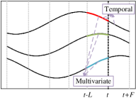
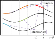
To forecast the next $F$ observations into the future, existing deep methods, including recurrent neural networks (wang2018multilevel, ; bai2019passenger, ), temporal convolutional networks (wu2019graph, ; campos2021unsupervised, ) and transformers (lim2021temporal, ; wu2021autoformer, ; zhou2021informer, ), all use similar mechanisms to train deep models. Given a time series, where observations are recorded from time 1 to $t$ these methods first split the entire time series into small subsequences of length $L+F$. These subsequences are then used as training data to learn a neural network model. Finally, the resulting model predicts a sequence of $F$ future observations when fed a sequence of $L$ observations. Intuitively, the better the learned models are at capturing correlations among the $L$ most recent observations and the $F$ future observations in the training data, the better their forecasting accuracy.

Following existing methods (bai2019passenger, ; wu2021autoformer, ; lim2021temporal, ; oreshkin2019n, ), we quantify the correlation between two observations by means of a similarity score between the two. We categorize correlations as being either temporal or multivariate. Temporal correlations refer to the influence of historical observations on future observations. For example, historical climate observations are helpful for climate prediction due to temporal correlations between historical and future observations. Temporal correlations are either local or global. As shown in Figure 1(a), local temporal correlations capture the influence of the $L$ most recent observations on the $F$ future observations. Global temporal correlations capture the influence of the observations in the entire time series, extending well before the most recent $L$ observations, as shown in Figure 1(b).

Multivariate correlations refer to the influence of one time series to another. For example, carbon dioxide time series correlate with temperature time series. As for temporal correlations, multivariate correlations may also be local or global. Local multivariate correlations are correlations among subsequences of the $L$ most recent observations from multiple time series, as shown in Figure 1(a). Global multivariate correlations are correlations between pairs of subsequences across the entire multivariate time series, as shown in Figure 1(b).

While the ability of a method to capture these correlations influences its forecasting accuracy significantly, capturing the correlations in a meaningful manner is difficult. We address two key challenges.

Challenge 1: It is difficult for existing deep methods to capture global temporal correlations due to how they are trained. In particular, the training data subsequences capture only local temporal correlations among $L$ historical and $F$ future observations. Once a time series is split into subsequences, the temporal alignment between the subsequences is lost. This makes it difficult to determine which subsequences are more important to future observations. Thus, existing methods fail to capture the global temporal correlations.

Challenge 2: It is difficult for existing methods to capture global multivariate correlations. Existing deep methods (wu2019graph, ; bai2020adaptive, ; cirstea2021enhancenet, ) utilize recurrent neural networks or transformers to capture local temporal correlations and utilize graph neural networks (hallac2017network, ; cao2020spectral, ) to capture local multivariate correlations by iteratively aggregating information from nearby time series. However, these methods fall short at capturing global multivariate correlations across an entire multivariate time series. Again, this is due to the training methodology used by recurrent neural networks and transformers when combined with graph neural networks—the entire multivariate time series are split into subsequences, whose correlations are then not available for training.

Proposed solution: To contend with the two challenges, we propose a novel deep autoregressive Gaussian process model called Autoregressive Gaussian Process (AutoGP) that integrates a different mechanism to train a forecasting model capable of capturing capture global temporal and global multivariate correlations. Specifically, we split the entire time series into subsequences. But instead of ignoring their global temporal and multivariate correlations, as do existing methods, we capture and consider these correlations during training. First, we use a sparse attention structure to capture local temporal correlations, as this structure has proven to be the most efficient and effective at capturing local temporal correlations (vaswani2017attention, ; zhou2021informer, ; DBLP:conf/ijcai/CirsteaG0KDP22, ). This attention structure also learns typical features of each subsequence. Next, we train models to learn global temporal and multivariate correlations by using Gaussian process kernels that can calculate correlations among subsequences using features extracted from them; these correlations are then used to predict future observations, and they also indicate the importance of a historical subsequence to a future observation.

Gaussian process kernels take well-defined analytic forms (wilson2013gaussian, ; tong2019discovering, ) that not only enable us to calculate correlations, or covariances, between pairs of subsequences, but also offer an opportunity to understand the correlations between subsequences using certain time series patterns, such as trend and seasonality, which offers good explainability. However, the traditional Gaussian process model uses a single pre-defined kernel function, e.g., a periodic kernel, for capturing the correlations among all time series, thus neglecting the diversity of correlations among different time series. For example, some time series may exhibit seasonality patterns, while others may exhibit show a combination of trend and periodicity patterns. Using a single and pre-defined kernel fails to capture dynamic and diverse correlations.

We introduce dynamic kernel learning as the core of the deep autoregressive Gaussian process to dynamically capture diverse correlations between any pair of subsequences across an entire multivariate time series. Instead of assigning a simple kernel manually in our deep autoregressive Gaussian process as prior knowledge, we introduce the novel notion of kernel association search (KAS) that is capable of exploring basic kernels and of efficiently discovering complex kernels, thus enabling the learning of global temporal and multivariate correlations in multivariate time series.

As all time series still use the same dynamically learned complex kernel to calculate global temporal and multivariate correlations, distinct aspects of individual correlations are still not captured well. Hence, we propose a learnable matrix of cross-variable weights for learning the importance of each entire time series to another. We then train models to learn diverse global temporal and multivariate correlations using the KAS learned kernel and the cross-variable weights. The resulting models are able to capture distinct global temporal and multivariate correlations.

Contributions: To the best of our knowledge, we propose the first deep learning method that uses a novel mechanism to train a forecasting model using entire time series to capture distinct temporal and multivariate correlations that are significant to multivariate time series forecasting, so as to achieve accurate forecasting. The paper offers the following contributions:

• We propose a novel deep autoregressive Gaussian process model to train using entire time series for multivariate time series forecasting, enabling models that can capture global temporal and multivariate correlations.

• We propose KAS, an efficient and dynamic kernel learning method, to find complex kernels, without requiring prior knowledge.

• We propose means of learning cross-variable weights to adjust the weights of global temporal and multivariate correlations, to capture the distinct correlations.

• We report on extensive experiments on public real-world data sets that offer insight into the prediction accuracy achieved. We visualize temporal and multivariate correlations learned from example time series.

2. Preliminaries

2.1. Problem Definition

We consider a multivariate time series $\mathbf{Y}\in\mathbb{R}^{t\times N}$, where $t$ denotes the number of observations, and $N$ indicates the number of time series or variables. An $F$-timestamps-ahead time series forecasting model $\mathcal{F}$ takes as input $L$ historical observations $\mathbf{y}_{t-L+1},\mathbf{y}_{t-L+2},...,\mathbf{y}_{t}$, with $L\ll t$, and predicts the $F$ future observations $\mathbf{y}_{t+1},\mathbf{y}_{t+2},...,\mathbf{y}_{t+F}$:

(1) $$\mathcal{F}_{\bm{\Gamma}}(\mathbf{y}_{t-L+1},\mathbf{y}_{t-L+2},...,\mathbf{y}_{t})=(\mathbf{y}_{t+1},\mathbf{y}_{t+2},...,\mathbf{y}_{t+F}),$$

where $\Gamma$ is a collection of learnable parameters and functions.

2.2. Gaussian Process

(a) Classical Gaussian Process

(b) Autoregressive Gaussian Process

Figure 2. Gaussian Processes

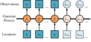
A Gaussian process is a joint Gaussian distribution consisting of a set of random variables (williams2006gaussian, ). Since training and inference for a Gaussian process are different, we introduce them separately.
Training: As Figure 2(a) shows, given $t$ training samples of location and observation pairs $(\mathbf{x},\mathbf{y})=\{(\mathrm{x}_{i},\mathrm{y}_{i})|i=1,2,...,t\}$ with additive, independent, and identically distributed Gaussian noise $\varepsilon$, we have $\mathrm{y}_{i}=f(\mathrm{x}_{i})\ +\ \varepsilon$. For simplicity, we use $f(\mathrm{x}_{i})$ and $f_{i}$ interchangeably, and we assume that $\mathbf{f}=f(\mathbf{x})=(f_{1},f_{2},...,f_{i},...,f_{t})$ is a collection of random variables. We assume a traditional Gaussian process and use ”locations” in the place of timestamps. A Gaussian process can be specified by its given priors—mean $\mu(\mathrm{x}_{i})$ and kernel function $k_{\theta}(\mathrm{x}_{i},\mathrm{x}_{j})$ that is parameterized by $\theta$. Specifically, $\theta$ can be given as prior values or learned through optimization (wilson2014covariance, ). The kernel function associates any pair of two random variables at locations $\mathrm{x}_{i}$ and $\mathrm{x}_{j}$. The mean and kernel functions are denoted as:

(2) $$\mu(\mathrm{x}_{i}) =\mathbb{E}[f(\mathrm{x}_{i})]$$

$$k_{\theta}(\mathrm{x}_{i},\mathrm{x}_{j}) =\mathbb{E}[(f(\mathrm{x}_{i})-\mu(\mathrm{x}_{i}))(f(\mathrm{x}_{j})-\mu(\mathrm{x}_{j}))],$$

giving rise to the Gaussian process:

(3) $$\mathbf{f}\sim\mathcal{GP}(\bm{\mu}(\mathbf{x}),\mathbf{K}(\mathbf{x},\mathbf{x})),$$

where $\bm{\mu}(\mathbf{x})=(\mu(\mathrm{x}_{1}),\mu(\mathrm{x}_{2}),...,\mu(\mathrm{x}_{t}))$ denotes the mean vector containing values for all training observations and $\mathbf{K}(\mathrm{x},\mathrm{x})$ is the covariance matrix that contains covariance values computed by kernel function $k_{\theta}(\mathrm{x}_{i},\mathrm{x}_{j})$ for each pair of training locations $\mathrm{x}_{i}$ and $\mathrm{x}_{j}$.

Although some studies refer to kernel functions and covariance matrices interchangeably, we distinguish between them. Specifically, we use kernel functions to represent the analytic forms of kernels that define priors on the Gaussian process distribution, and we use covariance matrices to represent the matrices of the covariance values computed by kernel functions. In addition, we set mean function $\mu$ to 0 as usual (williams2006gaussian, ).
Inference: Inference aims to predict random variables $\mathbf{f}_{*}=(f_{t+1},\\ f_{t+2},...)$ at test locations $\mathbf{x}_{*}=(\mathrm{x}_{t+1},\mathrm{x}_{t+2},...)$. Assuming noise $\varepsilon$ with variance $\sigma^{2}$, we formulate the joint distribution of the training observations $\mathbf{y}$ and the prediction random variables $\mathbf{f}_{*}$ under the priors, i.e., kernel functions, as follows.

(4) $$\begin{bmatrix}\mathbf{y}\\ \mathbf{f}_{*}\end{bmatrix}=\mathcal{N}\left(\begin{bmatrix}\bm{\mu}(\mathbf{x})\\ \bm{\mu}(\mathbf{x}_{*})\end{bmatrix},\begin{bmatrix}\mathbf{K}(\mathbf{x},\mathbf{x})+\sigma^{2}\mathbf{I}&\mathbf{K}(\mathbf{x},\mathbf{x}_{*})\\ \mathbf{K}(\mathbf{x}_{*},\mathbf{x})&\mathbf{K}(\mathbf{x}_{*},\mathbf{x}_{*})\end{bmatrix}\right),$$

where $\bm{\mu}(\mathbf{x})$ and $\bm{\mu}(\mathbf{x}_{*})$ denote the mean vectors and $\mathbf{K}(\mathbf{x},\mathbf{x})$, $\mathbf{K}(\mathbf{x}_{*},\mathbf{x})$, $\mathbf{K}(\mathbf{x},\mathbf{x}_{*})$, and $\mathbf{K}(\mathbf{x}_{*},\mathbf{x}_{*})$ are the covariance matrices. Then the conditional distribution of the prediction $\mathbf{f}_{*}$ has the form:

(5) $$\mathbf{f}_{*}|\mathbf{x},\mathbf{y},\mathbf{x}_{*}\sim\mathcal{N}(\mathbb{E}[\mathbf{f}_{*}],\mathrm{Cov}[\mathbf{f}_{*}]),$$

where

(6) $$\mathbb{E}[\mathbf{f}_{*}] =\bm{\mu}(\mathbf{x}_{*})+\mathbf{K}(\mathbf{x}_{*},\mathbf{x})[\mathbf{K}(\mathbf{x},\mathbf{x})+{\sigma}^{2}\mathbf{I}]^{-1}(\mathbf{y}-\bm{\mu}(\mathbf{x}))$$

$$\mathrm{Cov}[\mathbf{f}_{*}] =\mathbf{K}(\mathbf{x}_{*},\mathbf{x}_{*})-\mathbf{K}(\mathbf{x}_{*},\mathbf{x})[\mathbf{K}(\mathbf{x},\mathbf{x})+{\sigma}^{2}\mathbf{I}]^{-1}\mathbf{K}(\mathbf{x},\mathbf{x}_{*})$$

When we conduct point estimation, i.e., predict $\mathbf{y}_{*}$ given $\mathbf{x}_{*}$, we do not use the random variables $\mathbf{f}_{*}$ as the prediction values. Instead, we use the expectations $\mathbb{E}[\mathbf{f}_{*}]$ as the predictions, i.e., $\hat{\mathbf{y}}_{*}=(\hat{\mathrm{y}}_{t+1},\hat{\mathrm{y}}_{t+2},...)=(\mathbb{E}(f_{t+1}),\mathbb{E}(f_{t+2}),...)$, and the standards deviations $\mathrm{Cov}[\mathbf{f}_{*}]$ can be used to determine the confidence intervals.

2.3. Kernel Functions

Kernel functions are the priors used by the Gaussian process and denote the analytic forms of the functions that we are modeling. A kernel function is a function of $\mathrm{x}_{i}-\mathrm{x}_{j}$ (williams2006gaussian, ). A kernel function thus specifies the covariance between a pair of random variables, using a function of their location distance. For example, the squared exponential (SE) kernel is one of the most commonly used kernel functions in the Gaussian process. The observations $\mathrm{y}_{i}$ and $\mathrm{y}_{j}$ at two nearby locations $\mathrm{x}_{i}$ and $\mathrm{x}_{j}$ are expected to be close in a Gaussian process. In other words, the closer the locations are, the more similar the observations should be. Thus, the SE kernel function represents an interpretable pattern that captures short-term dependencies.

The SE kernel is defined as:

(7) $$k_{\theta}(\mathrm{x}_{i},\mathrm{x}_{j})=\sigma_{k}^{2}\mathrm{exp}\left(-\frac{||\mathrm{x}_{i}-\mathrm{x}_{j}||}{2l^{2}}\right),$$

where $\theta=\{\sigma_{k},l\}$ denotes the collection of parameters. Specifically, $\sigma_{k}$ denotes the scale factor of the covariance and $l$ represents the parameter length-scale. A shorter length-scale indicates that observations $\mathbf{y}$ vary more rapidly with locations $\mathbf{x}$.

Table 1. Basic Kernel Functions

Kernel Function	Interpretable Pattern	Analytic Form	Parameter(s)
SE	Short-term	$\sigma_{k}^{2}\mathrm{exp}\left(-\frac{||\mathrm{x}_{i}-\mathrm{x}_{j}||}{2l^{2}}\right)$	$l$
PER	Seasonality	$\sigma_{k}^{2}\mathrm{exp}\left(-\frac{2\mathrm{sin}^{2}(\frac{\pi|\mathrm{x}_{i}-\mathrm{x}_{j}|)}{p}}{l^{2}}\right)$	$l$,$p$
LIN	Trend	$\sigma_{k}^{2}(\mathrm{x}_{i}-c)(\mathrm{x}_{j}-c)$	$c$
RQ	Long-term	$\sigma_{k}^{2}\left(1+\frac{||\mathrm{x}_{i}-\mathrm{x}_{j}||}{2al^{2}}\right)^{-a}$	$l$,$a$ $>0$

Numerous kernel functions exist beyond the SE kernel function that describes the observations in an interpretable way. Table 1 lists basic kernel functions and the patterns they target. The analytic form of the PER kernel is a periodic function, enabling it to establish periodic correlations. The analytic form of the LIN kernel is a linear function, so it is able to capture linear correlations. The RQ kernel reduces to the SE kernel when the parameter $a\rightarrow\infty$ (rasmussen2003gaussian, ). The covariance captured via the RQ kernel decays more slowly with increasing distance than in the case of the SE kernel, as SE is the inverse of an exponential function and RQ is a power function with power $-a$. Therefore, the RQ kernel is capable of capturing long-term dependencies.

3. Autoregressive Gaussian Process

Traditional Gaussian process models are non-autoregressive and use timestamps as the Gaussian locations for regression tasks. In other words, they predict observation given their locations or timestamps. In contrast, time series forecasting requires an autoregressive method that predicts future observations given historical observations. Inspired by deep kernel learning methods (al2017learning, ), we define a deep autoregressive Gaussian process for multivariate time series forecasting that recursively predicts each future observation given a subsequence of historical observations. Further, the global temporal correlation in the full time series is modeled via Gaussian process kernel functions. More specifically, this process contains two procedures—training and inference.

Training: In order to establish the global temporal correlations of time series as exemplified in  Figure 2(b), the multivariate time series $\mathbf{Y}\in\mathbb{R}^{t\times N}$ is sliced into a series $\mathbf{M}$ of $B$ subsequences by moving a time window of length $L$ in steps of length $\Delta$: $\mathbf{M}=(\mathbf{M}_{1},\mathbf{M}_{2},...,\mathbf{M}_{i},...,\mathbf{M}_{B})$, where $\mathbf{M}_{i}\in\mathbb{R}^{L\times N}$ and $B=(t-L+1)/\Delta$. The $i$-th subsequence $\mathbf{M}_{i}$ is denoted as:

(8) $$\mathbf{M}_{i}=(\mathbf{y}_{(i-1)\Delta+1},\mathbf{y}_{(i-1)\Delta+2},...,\mathbf{y}_{(i-1)\Delta+L})$$

Like in the traditional Gaussian process training, we define a future observation as $\mathbf{y}_{(i-1)\Delta+L+1}=\mathbb{E}(f_{i})$, where $f_{i}=f(g_{\mathbf{w}}(\mathbf{M}_{i}))$ and $g_{\mathbf{w}}(\cdot)$ is a neural network, as shown in Figure 2(b). To enable time series forecasting, we build a temporal correlation between a historical subsequence $\mathbf{M}_{i}$ and a predicted observation $\mathbf{y}_{(i-1)\Delta+L+1}$. We then match $g_{\mathbf{w}}(\mathbf{M}_{i})$ and $\mathbf{y}_{(i-1)\Delta+L+1}$ with $\mathrm{x}_{i}$ and $\mathrm{y}_{i}$ in the training stage as shown in subsection 2.2 and formulate the autoregressive Gaussian process as follows.

(9) $$(f_{1},...,f_{i},...,f_{B})\sim\mathcal{GP}(\bm{\mu}(g_{\mathbf{w}}(\mathbf{M})),\mathbf{K}(g_{\mathbf{w}}(\mathbf{M}),g_{\mathbf{w}}(\mathbf{M}))),$$

where $\bm{\mu}(g_{\mathbf{w}}(\mathbf{M}))=(\mu(g_{\mathbf{w}}(\mathbf{M}_{1})),...,\mu(g_{\mathbf{w}}(\mathbf{M}_{B})))$ is the mean vector, and $\mathbf{K}(g_{\mathbf{w}}(\mathbf{M}),g_{\mathbf{w}}(\mathbf{M}))$ is the covariance matrix.

To achieve better time series forecasting accuracy, our goal is to learn the AutoGP model that contains three parts. The first is a neural network $g_{\mathbf{w}}(\cdot)$ that transforms the subsequences $\mathbf{M}$ into Gaussian locations. The second is a final kernel function $K_{\bm{\theta}}$ that is an association of kernel functions guided by a learnable cross-variable weight matrix $\mathbf{D}$, which is the third part. Here $g_{\mathbf{w}}(.)$ is parameterized by $\mathbf{w}$, and $K_{\bm{\theta}}$ is parameterized by $\bm{\theta}$. Thus, the model has parameters $\Gamma=\{\mathbf{w},K,\bm{\theta},\mathbf{D}\}$ and can be stated as follows.

(10) $$AutoGP_{\bm{\Gamma}}(\mathbf{M}_{1},...,\mathbf{M}_{B}) =(\mathbf{y}_{L+1},...,\mathbf{y}_{t})$$

We train the model using $\mathbf{M}_{1},...,\mathbf{M}_{B}$, and $\mathbf{y}_{L+1},...,\mathbf{y}_{t}$, in order to learn ${\mathbf{w}}$, $K$, ${\bm{\theta}}$, and $\mathbf{D}$.

Inference: To iteratively infer the future $F$ observations, as illustrated in subsection 2.2, we use traditional Gaussian process inference. Specifically, in the first iteration, we match $g_{\mathbf{w}}(\mathbf{M}_{B+1})$, where $\mathbf{M}_{B+1}=\mathbf{y}_{t-L+1},...,\mathbf{y}_{t}$, and $\hat{\mathbf{y}}_{t+1}$ with $\mathrm{x}_{t+1}$ and $\hat{\mathrm{y}}_{t+1}$, and thus infer $\mathbf{y}_{t+1}$ using Equation 4–6, as shown in Figure 2(b). Unlike in traditional Gaussian process inference that takes arbitrary future locations as input and predicts their observations, the autoregressive Gaussian process predicts iteratively, as follows.

(11) $$\mathit{AutoGP}_{\bm{\Gamma}}(\mathbf{y}_{t-L+1},...,\mathbf{y}_{t}) =\mathbf{\hat{y}}_{t+1}$$

$$\mathit{AutoGP}_{\bm{\Gamma}}(\mathbf{y}_{t-L+2},...,\mathbf{\hat{y}}_{t+1}) =\mathbf{\hat{y}}_{t+2}$$

$$......$$

$$\mathit{AutoGP}_{\bm{\Gamma}}(\mathbf{\hat{y}}_{t-L+F},...,\mathbf{\hat{y}}_{t+F-1}) =\mathbf{\hat{y}}_{t+F},$$

where the sequence $\mathbf{\hat{y}}_{t+1},\mathbf{\hat{y}}_{t+2},...,\mathbf{\hat{y}}_{t+F}$ denotes $F$ predictions. Figure 3 provides an overview of the proposed solution.

Figure 3. Solution Overview

4. Methodology

Figure 4. AutoGP Training

4.1. Framework

The training of the proposed AutoGP deep kernel model framework is illustrated in Figure 4. The framework takes as input subsequences $\mathbf{M}=(\mathbf{M}_{1},\mathbf{M}_{2},...,\mathbf{M}_{i},...,\mathbf{M}_{B})$, where $\mathbf{M}_{i}\in\mathbb{R}^{L\times N}$, and outputs predictions $\mathbf{y}_{L+1},...,\mathbf{y}_{L+i},...,\mathbf{y}_{L+j},...,\mathbf{y}_{t}$ for training.

The framework adopts a Gaussian process that models the temporal correlations of the whole time series. The first component, attention-based Gaussian location learning, takes as input $\mathbf{M}$ and outputs representations $\mathbf{H}=(\mathbf{h}_{1},...,\mathbf{h}_{i},...,\mathbf{h}_{j},...,\mathbf{h}_{B})$, where $\mathbf{h}_{i}\in\mathbb{R}^{N}$ represents the location of a Gaussian process, cf. Figure 4(a). We use patch-attention modules to capture the local temporal correlations within subsequence $\mathbf{M}_{i}$ and transfer subsequences $\mathbf{M}$ to Gaussian process locations $\mathbf{H}$ to capture the global temporal correlations.

The second component, dynamic kernel learning, aims at dynamically learning and searching the association of kernels to take into account the diverse patterns in multivariate time series. The dynamic kernel learning starts from a basic kernel set $\mathcal{K}$. In Figure 4(b), we assume $\mathcal{K}=\{k_{1},...,k_{4}\}$, corresponding to the four kernel functions shown in Table 1. The component automatically expands and learns potential new kernels via kernel association search (KAS) to achieve the final kernel function $K_{\theta}$, which is an association of basic kernels, e.g., $k_{1}$ and $k_{2}$, and expanded kernels, e.g., $k_{S}$. For simplicity, we denote $K_{\theta}$ as $K$.

Figure 4(c) shows the third component in the framework, multivariate covariance learning, that aims to capture the global multivariate correlations among variables. Taking the Gaussian locations $\mathbf{H}$ and the learned kernel $K$ as input, the component calculates the multivariate covariance matrix $\mathbf{K}(\mathbf{H},\mathbf{H})$ among Gaussian locations $\mathbf{H}$ via the learned kernel $K$. For simplicity, we denote $\mathbf{K}(\mathbf{H},\mathbf{H})$ as $\mathbf{K}$. Specifically, since the learned kernel is shared by all variables, the framework first computes a shared-kernel covariance matrix $\mathbf{C}(\mathbf{H},\mathbf{H})$, denoted as $\mathbf{C}$ for simplicity, that captures the global multivariate correlation via the shared kernel $K$. Next, it learns the cross-variable weights matrix $\mathbf{D}\in\mathbb{R}^{N^{2}}$ that captures the importance between each pair of variables. Finally, the framework calculates $\mathbf{K}$, which is the Hadamard product of $\mathbf{C}$ and $\mathbf{D}$, to model the distributions in the Gaussian process.

When used for inference, the framework takes as input a test subsequence and outputs $F$ future observations using Equations 6 and 11.

4.2. Attention-based Gaussian Location Learning

The framework utilizes attention structures to capture the local temporal correlations among observations in subsequence $\mathbf{M}_{i}$ and utilizes the Gaussian process to construct global temporal correlations among all subsequences $\mathbf{M}$.

Specifically, we utilize patch-attention (DBLP:conf/ijcai/CirsteaG0KDP22, ) as $g_{\mathbf{w}}(\cdot)$ to transform the input subsequences $\mathbf{M}$ to attention-based Gaussian locations $\mathbf{H}$ since patch-attention is the most efficient and effective state-of-the-art attention structure. $\mathbf{H}$ are also used as representations of $\mathbf{M}$. The intuition is that the representations capture typical features well, thus enabling higher prediction accuracy than when using timestamps of the time series as the input to the Gaussian process, since the Gaussian processes are able to capture complex temporal dependencies more easily in latent space (al2017learning, ).

A patch-attention is a triangular component—cf. Figure 4(a). Each patch-attention module takes as input a subsequence $\mathbf{M}_{i}\in\mathbb{R}^{L\times N}$ and outputs a Gaussian location $\mathbf{h}_{i}\in\mathbb{R}^{N}$. Unlike self-attention (vaswani2017attention, ) that computes an attention score between each pair of observations within each $\mathbf{M}_{i}$, patch-attention breaks down the $L$ observations into $P=L/\delta$ patches, where $\delta$ is the patch size. For the $p$-th patch $\mathbf{M}_{i,p}$ of subsequence $\mathbf{M}_{i}$, patch-attention defines a pseudo observation $\mathbf{T}_{i,p}\in\mathbb{R}^{N\times d}$, which is a learnable data placeholder. Patch-attention computes an attention score between the pseudo observation $\mathbf{T}_{i,p}$ and each observation in patch $\mathbf{M}_{i,p}$ and outputs a representation $\mathbf{O}_{i,p}$ of $\mathbf{M}_{i,p}$, given as follows.

(12) $$\mathbf{O}_{i,p}=\mathit{PA}(\mathbf{T}_{i,p},\mathbf{M}_{i,p})=\left\{\varphi\left(\frac{\mathbf{T}_{i,p}^{n}(\mathbf{M}_{i,p}^{n}\mathbf{W}_{K})^{\top}}{\sqrt{d_{k}}}\right)(\mathbf{M}_{i,p}^{n}\mathbf{W}_{V})\right\}_{n=1}^{N},$$

where $\mathit{PA}(\cdot)$ denotes the patch-attention, $\varphi(\cdot)$ denotes a $\mathit{softmax}$ activation function, $\mathbf{W}_{K}$ and $\mathbf{W}_{V}$ represent learned wights, $d_{k}$ is the number of attention heads, and $N$ is the number of variables. The decrease of connections enables the model to capture only the useful information and reduce the complexity of the attention layer.

Since the original $p$-th patch $\mathbf{M}_{i,p}$ is transformed to $\mathbf{O}_{i,p}$, all the outputs $(\mathbf{O}_{i,1},\mathbf{O}_{i,2},...,\mathbf{O}_{i,p},...,\mathbf{O}_{i,P})$ are concatenated into a vector that is then passed to a transformation neural network. This procedure is represented as follows.

(13) $$\mathbf{h}_{i}=\mathit{MLP}(\mathbf{O}_{i,1},\mathbf{O}_{i,2},...,\mathbf{O}_{i,p},...,\mathbf{O}_{i,P}),$$

where $\mathit{MLP}(\cdot)$ is a 3-layer fully connected neural network (zhou2021informer, ) and $\mathbf{h}_{i}$ is an attention-based Gaussian location. So far, we have obtained the representation series $\mathbf{H}=(\mathbf{h}_{1},...,\mathbf{h}_{i},...,\mathbf{h}_{j},...,\mathbf{h}_{B})$ to be used as the locations in the Gaussian process. The formulation of the Gaussian layer is as follows.

(14) $$(f_{1},...,f_{i},...,f_{j},...,f_{B})\sim\mathcal{GP}(\bm{\mu}(\mathbf{H}),\mathbf{K}(\mathbf{H},\mathbf{H})),$$

where $\bm{\mu}(\mathbf{H})=(\mu(\mathbf{h_{1}}),...,\mu(\mathbf{h_{i}}),...,\mu(\mathbf{h_{j}}),...,\mu(\mathbf{h_{B}}))$ and $\mathbf{K}(\mathbf{H},\mathbf{H}))$ are the mean vector and the covariance matrix.

(a) Greedy Kernel Search

(b) Kernel Association Search

Figure 5. Kernel Search Methods

4.3. Dynamic Kernel Learning

Instead of using a simple and fixed kernel function to model the global temporal correlations among subsequences $\mathbf{M}$, which fails to capture the diversity among time series, such as combinations of a growing trends and periodic patterns, we propose to learn a kernel function $K$ to capture such diversity. This is called dynamic kernel learning, and it encompasses kernel association that defines the rules of structural exploration of new kernels and kernel search that applies two kernel search methods to obtain the final kernel $K$.

4.3.1. Kernel Association

A new and more complex kernel function can be obtained by the addition and multiplication of existing kernel functions because positive semi-definite covariance matrices are closed under addition and multiplication (duvenaud2013structure, ).

Lemma 4.1.

Let $k_{1}$ and $k_{2}$ be kernels and let let $+$ and $\times$ denote addition and multiplication, respectively. Then $+$, $k_{1}+k_{2}$ and $k_{1}\times k_{2}$ are kernels.

Lemma 4.1 allows us to expand basic kernels into high-order kernels with power larger than 2. For example, LIN is a basic kernel, and LIN² is a 2-order kernel. The basic kernel LIN denotes a trend pattern, while the high-order kernel LIN² denotes a quadratic pattern. When a high-order kernel is combined with basic kernels into a final kernel $K$, it exhibits a more complex analytic form than do the basic kernels. We call this procedure kernel association (motai2014kernel, ). The intuition is that kernels with different orders should be included in $K$ because basic kernels capture general patterns of time series, while higher order kernels capture higher order information. As more higher order kernels are included in $K$, $K$ approximates the real patterns better. This is similar to polynomial approximation (hastie2009elements, ).

Specifically, we define a basic kernel set $\mathcal{K}=\{k_{1},k_{2},...,k_{|\mathcal{K}|}\}$, where $k_{i}$ denotes a kernel in $\mathcal{K}$, and $|\mathcal{K}|$ is the number of kernels in $\mathcal{K}$. Then we define an operation set $\mathcal{O}=\{+,\times\}$. Our goal is to discover a suitable final kernel $K$, which is an association of basic and expanded, high-order kernels obtained via operations in $\mathcal{O}$.

4.3.2. Kernel Search

We proceed to introduce two kernel search methods—greedy kernel search, used by existing models (grosse2012exploiting, ; duvenaud2013structure, ; lloyd2014automatic, ; tong2019discovering, ) and KAS, a kernel association search method.

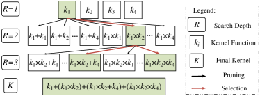
Greedy Kernel Search: As shown in Figure 5(a), assuming a basic kernel set $\mathcal{K}=\{k_{1},k_{2},k_{3},k_{4}\}$, an operation set $\mathcal{O}=\{+,\times\}$, and a search depth $R=3$, the goal of greedy kernel search is to discover a final kernel $K$.

In the first iteration, the method randomly picks a basic kernel in $\mathcal{K}$, say $k_{1}$, and then starts by setting $K=k_{1}$. Then it validates the forecasting loss, thus deriving a validation loss $\mathcal{L}_{val}$. Next, it checks whether associating $K$ with each other basic kernel, say $k_{i}$, i.e., obtaining $K=K+k_{i}$, is able to reduce $\mathcal{L}_{val}$. If so, $k_{i}$ is selected in the iteration. Assume that only $k_{1}$ is selected in the first iteration, as indicated by the green block in Figure 5(a). This means that the main pattern learned is $k_{1}$ and that $K=k_{1}$. In the second iteration, the method extends each kernel selected at the first iteration, e.g., $k_{1}$, with $|\mathcal{O}||\mathcal{K}|$ new kernels, where $|\mathcal{O}|$ is the number of operations in $\mathcal{O}$, and form candidates $(k_{1}+k_{1}),(k_{1}+k_{2}),...,(k_{1}\times k_{4})$. Similar in the first iteration, greedy search is used to validate each candidate kernel, and a kernel is selected if its association with $K$ lowers $\mathcal{L}_{val}$. For example, candidate $k1\times k2$ is selected, and $K=k_{1}+(k_{1}\times k_{2})$ after the second iteration is done. Iterations occur, until $R$ is reached. For example, when $R=3$, two higher order kernels are associated with $K$. The final kernel $K$ is the addition of the kernels selected at all levels.

However, although greedy kernel search discovers and expands kernels automatically, forecasting loss validation must be performed each time a candidate kernel is checked, which leads to time complexity $O(|\mathcal{K}|^{R})$, which is high.

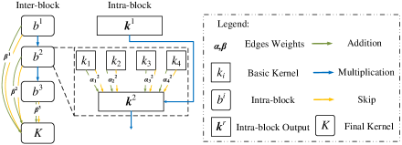
Kernel Association Search: To avoid the high complexity of greedy kernel search, we design a novel 2-level kernel search method (KAS), inspired by neural architecture search methods (liu2018darts, ; wu2021autocts, ), that includes intra-block and inter-block kernel associations, as shown in Figure 5(b). Each intra-block association $b^{r}$ intends to construct an $r$-th order kernel $\bm{k}^{r}$, and the inter-block sums kernels $\bm{k}^{1},...,\bm{k}^{R}$ to obtain the final kernel $K$.

Each intra-block association $b^{r}$ involves addition followed by multiplication. The input to the addition part is a set of basic kernels $\mathcal{K}=\{k_{1},k_{2},...,k_{|\mathcal{K}|}\}$, and the output is a kernel $\bm{k}^{r}$ that sums basic kernels. The input to the multiplication part is $\bm{k}^{r-1}$ and $\bm{k}^{r}$ derived from the addition part, and the output is still $\bm{k}^{r}$ that denotes a high-order kernel, by applying $\bm{k}^{r}=\bm{k}^{r-1}\times\bm{k}^{r}$.

In the addition part, each pair of a basic kernel $k_{i}$ and $\bm{k}^{r}$, we have an edge set $\mathcal{E}$ that contains operations used to connect $k_{i}$ and $\bm{k}^{r}$. To enable intra-block addition, we define $\mathcal{E}=\{+,\mathit{skip}\}$, where the edge $+$ indicates that $k_{i}$ should be included to form $\bm{k}^{r}$, and the edge $\mathit{skip}$ means that $k_{i}$ should be omitted. For example, for $\bm{k}^{r}=k_{1}+k_{2}$, an edge $+$ is selected between $k_{1}$ and $\bm{k}^{r}$ and between $k_{2}$ and $\bm{k}^{r}$; an edge $\mathit{skip}$ is selected between $k_{3}$ and $\bm{k}^{r}$ and between $k_{4}$ and $\bm{k}^{r}$. Next, ${\alpha}_{i,j}^{r}$ denotes the weight on the $j$-th edge between the $i$-th basic kernel and $\bm{k}^{r}$. Thus, we have a set of weights $\bm{\alpha}_{i}^{r}=\{\alpha_{i,1}^{r},...,\alpha_{i,j}^{r},...,\alpha_{i,|\mathcal{E}|}^{r}\}$ between $k_{i}$ and $\bm{k}^{r}$. KAS selects either addition or skip by optimizing weights $\bm{\alpha}_{i}^{r}$. Specifically, if $\alpha_{i,j}^{r}$ is the largest weight in $\bm{\alpha}_{i}^{r}$, KAS selects the $j$-th edge between $k_{i}$ and $\bm{k}^{r}$. Intra-block optimization is denoted as follows.

(15) $$\bm{k}^{r}=\sum_{i=1}^{|\mathcal{K}|}\sum_{j=1}^{|\mathcal{E}|}\frac{\mathrm{exp}(\alpha_{i,j}^{r})}{\sum_{j=1}^{|\mathcal{E}|}\mathrm{exp}(\alpha_{i,j}^{r})}e_{j}(k_{i}),$$

where $e_{j}$ denotes the $j$-th operation in $\mathcal{E}$.

In the multiplication part, we produce $\bm{k}^{r}=\bm{k}^{r-1}\times\bm{k}^{r}$, when $r>1$, to generate high-order kernels. For intra-block $b^{1}$, the multiplication part is denoted as $\bm{k}^{1}=\bm{k}^{0}\times\bm{k}^{1}$, and we define $\bm{k}^{0}=1$. As shown in Figure 5(b), there is a multiplication edge from $b^{1}$ to $b^{2}$, which indicates the multiplication operation $\bm{k}^{1}\times\bm{k}^{2}$. For example, assuming that $\bm{k}^{1}=k_{1}+k_{2}$ and $\bm{k}^{2}=k_{3}$ are produced by $b^{1}$ and $b^{2}$, respectively, we update $\bm{k}^{2}=\bm{k}^{1}\times\bm{k}^{2}=(k_{1}+k_{2})\times k_{3}$ to get a higher-order kernel.

An inter-block contains $R$ intra-blocks. The input is a set of kernels $\{\bm{k}^{1},...,\bm{k}^{r},...,\bm{k}^{R}\}$ that are learned in intra-blocks, and the output is the final kernel $K$, which is an association of basic and high-order kernels. To enable inter-block addition, we again use $\mathcal{E}=\{+,\mathit{skip}\}$, where a $+$ edge indicates that $b^{r}$ should be included in $K$, and a $\mathit{skip}$ edge means that $b^{r}$ should not be included. For example, for $K=\bm{k}^{1}+\bm{k}^{2}$, where $\bm{k}^{1}=k_{1}+k_{2}$, and $\bm{k}^{2}=(k_{1}+k_{2})\times k_{3}$, a $+$ edge is selected between $\bm{k}^{1}$ and $K$ and between $\bm{k}^{2}$ and $K$, and a $\mathit{skip}$ edge is selected between $\bm{k}^{3}$ and $K$. Further, $K=k_{1}+k_{2}+(k_{1}+k_{2})\times k_{3}$ can be distributed as $K=k_{1}+k_{2}+k_{1}\times k_{3}+k_{2}\times k_{3}$. We use ${\beta}_{j}^{r}$ to denote the weight on the $j$-th edge between the $r$-th intra-block and $K$. Thus, we have a set of weights $\bm{\beta}^{r}=\{\beta_{1}^{r},...,\beta_{j}^{r},...,\beta_{|\mathcal{E}|}^{r}\}$ between $b^{r}$ and $K$. KAS selects addition or skip operations by optimizing weights $\bm{\beta}^{r}$. Specifically, if $\beta_{j}^{r}$ is the largest value in $\bm{\beta}^{r}$, KAS selects the $j$-th edge between $b^{r}$ and $K$. Inter-block optimizations are formulated as follows.

(16) $$K=\sum_{r=1}^{R}\sum_{j=1}^{|\mathcal{E}|}\frac{\mathrm{exp}(\beta_{j}^{r})}{\sum_{j=1}^{|\mathcal{E}|}\mathrm{exp}(\beta_{j}^{r})}e_{j}(\bm{k}^{r})$$

We also notice that kernels are not equally important. Thus, as shown in Figure 4(b), after KAS completes kernel selection, we retrain the model and learn weights $\bm{\zeta}=\{\zeta_{1},\zeta_{2},...,\zeta_{S}\}$. A higher weight indicates that the kernel is more important when calculating correlations.

(17) $$K=\zeta_{1}k_{1}+\zeta_{2}k_{2}+...+\zeta_{s}k_{s}+...+\zeta_{S}k_{S},$$

where $\zeta_{s}$ denotes the weight of $s$-th kernel $k_{s}$ in $K$.

The kernel selection is completed in one iteration without traversing the search tree as done in the greedy strategy. The the time complexity is $O(|\mathcal{K}|R)$. KAS involves only one instance of forecasting validation loss computation, thereby reducing the time complexity.

4.4. Multivariate Covariance Learning

We use the multivariate covariance matrix $\mathbf{K}$ to capture the correlations between each two subsequences of different variables. In order to learn $\mathbf{K}$, we first calculate a shared-kernel covariance matrix $\mathbf{C}$ via a multi-task Gaussian process (parra2017spectral, ), a Gaussian process that handles multiple variables, and then we learn a matrix $\mathbf{D}$ that captures the cross-variable weights between each pair of variables. Finally, we get the multivariate covariance matrix $\mathbf{K}$ as the Hadamard product of $\mathbf{C}$ and $\mathbf{D}$ for the correlations between any two subsequences of any two variables.

4.4.1. Shared-kernel Covariance

The shared-kernel covariance matrix $\mathbf{C}\in\mathbb{R}^{B^{2}\times N^{2}}$ is learned from the attention-based Gaussian locations $\mathbf{H}$ and the kernel function $K$. An element $\mathbf{C}^{m,n}\in\mathbb{R}^{B^{2}}$ in $\mathbf{C}$ denotes the covariance between the $m$-th variable and the $n$-th variable in $\mathbf{H}$:

(18) $$\mathbf{C}=\left[\begin{matrix}\mathbf{C}^{1,1}&\mathbf{C}^{1,2}&\cdots&\mathbf{C}^{1,N}\\ \mathbf{C}^{2,1}&\mathbf{C}^{2,2}&\cdots&\vdots\\ \vdots&\vdots&\ddots&\vdots\\ \mathbf{C}^{N,1}&\mathbf{C}^{N,2}&\cdots&\mathbf{C}^{N,N}\\ \end{matrix}\right]$$

Element $\mathbf{C}^{m,n}$ is also a matrix, an element $\mathbf{C}_{i,j}^{m,n}$ of which denotes the temporal covariance between the $i$-th subsequence of the $m$-th variable $\mathbf{h}_{i}^{m}$ and the $j$-th subsequence of the $n$-th variable $\mathbf{h}_{j}^{n}$. Assuming that the final kernel $K$ contains $S$ kernel functions, we have:

(19) $$\mathbf{C}_{i,j}^{m,n}=K(\mathbf{h}_{i}^{m},\mathbf{h}_{j}^{n})=\sum_{s=1}^{S}\zeta_{s}k_{s}(\mathbf{h}_{i}^{m},\mathbf{h}_{j}^{n})$$

4.4.2. Cross-variable Weights

The multi-task Gaussian process captures the multivariate covariance by means of a single shared kernel function $K$. As this limits the capability of capturing diverse correlations between variables, we propose a learnable matrix $\mathbf{D}\in\mathbb{R}^{N^{2}}$ that represents the cross-variable weights, thus extending the capabilities of a single shared kernel. To ensure that covariance matrix $\mathbf{D}$ is positive semi-definite, we define $\mathbf{D}$ as follows.

(20) $$\mathbf{D}=\mathbf{D^{\prime}}(\mathbf{D}^{\prime})^{\top}+diag(\bm{\lambda}),$$

where $\mathbf{D}^{\prime}\in\mathbb{R}^{N\times V}$ is a low-rank matrix, $V\ (V<N)$ represents the number of non-zero columns in $\mathbf{C}$, and $\bm{\lambda}$ is a non-negative vector.

The multivariate covariance matrix $\mathbf{K}$ is calculated through the Hadamard product of the shared-kernel covariance and the cross-variable weights:

(21) $$\mathbf{K} =\sum_{s=1}^{S}\zeta_{s}\left[\begin{matrix}d_{1,1}k_{s}(\mathbf{h}^{1},\mathbf{h}^{1})&\cdots&d_{1,N}k_{s}(\mathbf{h}^{1},\mathbf{h}^{N})\\ d_{2,1}k_{s}(\mathbf{h}^{2},\mathbf{h}^{1})&\cdots&\vdots\\ \vdots&\ddots&\vdots\\ d_{N,1}k_{s}(\mathbf{h}^{N},\mathbf{h}^{1})&\cdots&d_{N,N}k_{s}(\mathbf{h}^{N},\mathbf{h}^{N})\\ \end{matrix}\right]$$

$$=\mathbf{D}\odot\mathbf{C},$$

where $d_{m,n}$ denotes the weight of $\mathbf{C}^{m,n}$ that constructs the cross-variable correlation between any pairs of variables. Thus, the correlation between any two subsequences of two variables also considers the distinct correlation between the two variables. Matrix $\mathbf{K}$ will be fed into the multi-task Gaussian process for training and inference.

4.5. Training and Optimization

Next, we consider the optimization of parameters in the AutoGP framework. As the multivariate time series forecasting problem is formulated as a Gaussian process, we use negative log marginal likelihood (wilson2016stochastic, ) rather than the general regression loss function from deep learning to optimize parameters.

The negative log marginal likelihood loss function is denoted as:

(22) $$\mathcal{L}=-[\mathbf{y}^{\top}(\mathbf{K}+{\sigma}^{2}I)^{-1}\mathbf{y}+\log{\det|\mathbf{K}+{\sigma}^{2}I|}]+\mathit{const},$$

where $\mathbf{y}$ denotes a series of observations, $\mathbf{K}$ represents a learned covariance matrix with analytic form $K$, and $\sigma^{2}$ is the variance of noise. Next, $\mathbf{y}^{\top}(\mathbf{K}+{\sigma}^{2}I)^{-1}\mathbf{y}$ is a positive semi-definite covariance matrix, $\mathrm{det}|\cdot|$ is the determinant of the argument matrix, and $const$ is a constant term.

The framework learns the analytic form of kernel function $K$ achieved via KAS and parameters $\bm{\Gamma}=\{\mathbf{w},K,\bm{\theta},\mathbf{D}\}$, where $\mathbf{w}$ denotes the learnable weights in the patch-attention, $\bm{\theta}$ represents the collection of parameters of the kernel $K$, which includes $\bm{\alpha}$, $\bm{\beta}$, $\bm{\zeta}$, and other parameters related to kernels, and $\mathbf{D}$ indicates the cross-variable weights. Specifically, the cross-variable weights $\mathbf{D}$ is a positive semi-definite matrix, and kernel computation is closed under the Hadamard product operation. Thus, the optimization of $\mathbf{D}$ and $\bm{\theta}$ represents the parameter optimization of kernel $K$. Therefore, $\mathbf{D}$ is regarded as a covariance matrix, and the optimization procedures of $\mathbf{D}$ and $\bm{\theta}$ are combined. We let $\bm{\Theta}=\{\bm{\theta},\mathbf{D}\}$. The framework then learns parameters $\bm{\Theta}$ and $\mathbf{w}$ jointly via back-propagation using loss function $\mathcal{L}$ and gradient descent. The partial derivative $\frac{\partial{\mathcal{L}}}{\partial{\bm{\Theta}}}$ stated below is proved by an existing study (wilson2016deep, ).

(23) $$\frac{\partial{\mathcal{L}}}{\partial{\bm{\Theta}}}=\frac{1}{2}\mathrm{tr}\left(\left[\mathbf{K}^{-1}\mathbf{y}\mathbf{y}^{\top}\mathbf{K}^{-1}-\mathbf{K}^{-1}\right]\frac{\partial{\mathbf{K}}}{\partial{\bm{\Theta}}}\right)$$

The partial derivative $\frac{\partial{\mathcal{L}}}{\partial{\mathbf{w}}}$ of the parameters $\mathbf{w}$ is also proved by an existing study (al2017learning, ).

(24) $$\frac{\partial{\mathcal{L}}}{\partial{\mathbf{w}}}= \frac{1}{2}\sum_{m,n}\sum_{i,j}(\mathbf{K}(\mathbf{h}_{i}^{m},\mathbf{h}_{j}^{n})^{-1}\mathbf{y}\mathbf{y}^{\top}\mathbf{K}(\mathbf{h}_{i}^{m},\mathbf{h}_{j}^{n})^{-1}-\mathbf{K}(\mathbf{h}_{i}^{m},\mathbf{h}_{j}^{n})^{-1})$$

$$\left\{\left(\frac{\partial{\mathbf{K}(\mathbf{h}_{i}^{m},\mathbf{h}_{j}^{n})}}{\partial{\mathbf{h}^{m}_{i}}}\right)^{\top}\frac{\partial{\mathbf{h}^{m}_{i}}}{\partial{\mathbf{w}}}+\left(\frac{\partial{\mathbf{K}(\mathbf{h}_{i}^{m},\mathbf{h}_{j}^{n})}}{\partial{\mathbf{h}^{n}_{j}}}\right)^{\top}\frac{\partial{\mathbf{h}^{n}_{j}}}{\partial{\mathbf{w}}}\right\}$$

Then we update the parameters using gradient descent as follows.

(25) $$\bm{\Theta} =\bm{\Theta}-\eta\frac{\partial{\mathcal{L}}}{\partial{\bm{\Theta}}}$$

$$\mathbf{w} =\mathbf{w}-\eta\frac{\partial{\mathcal{L}}}{\partial{\mathbf{w}}},$$

where $\eta$ is a learning rate that is used to control the learning speed.

5. EXPERIMENTAL STUDY

5.1. Experimental Setup

5.1.1. Datasets and Evaluation Metrics

We conduct experiments on four benchmark datasets.

M4: The M4 (makridakis2018m4, ) univariate time series dataset contains 100k time series and consists of data frequently encountered in business, finance, and industry forecasting. The M4 time series show trend and seasonality patterns. The sampling frequencies include yearly, quarterly, monthly, weekly, daily, and hourly.
ACSF1: The univariate time series dataset ACSF1 is drawn from the UCR repository (dau2019ucr, ). It contains 200 power consumption time series from typical appliances, and the time series length is 1460. Time series in ACSF1 embody a short-period seasonality pattern. In addition, these time series contain points with abrupt changes, caused by appliances being turned on or off.
SML2010: A multivariate time series dataset, SML2010 (zamora2014line, ) contains 4137 observations, each with 17 numerical variables that are recorded by indoor sensors to enable temperature forecasting. The target variable—Temperature Comedor has a seasonality pattern.
Electricity: Again a multivariate time series dataset, Electricity captures the electricity consumption of 370 users. The electricity consumption of different users is regarded as a different variable.

Table 2. Statistics of Datasets

Dataset	$N$	Length	Split Ratio	Input $L$	Output $F$
M4-Yearly	23,000	19$\sim$841	7:1:2	12	6
M4-Quarterly	24,000	24$\sim$874	7:1:2	16	8
M4-Monthly	48,000	60$\sim$2,812	7:1:2	36	18
M4-Weekly	359	93$\sim$2,610	7:1:2	26	13
M4-Daily	4,227	107$\sim$9,933	7:1:2	28	14
M4-Hourly	414	748$\sim$1,008	7:1:2	96	48
ACSF1	200	1,460	7:1:2	12	12
SML2010	17	4,137	3200:400:537	3$\sim$24	3$\sim$24
Electricity	370	26,304	7:1:2	3$\sim$24	3$\sim$24

Table 2 summarizes the statistical details of the aforementioned datasets, where $N$ denotes the number of time series or variables, ”Length” denotes the length of time series, ”Split Ratio” represents the ratio of train-validation-test for the dataset, ”Input $L$” and ”Output $F$” stand for the length of the historical horizon $L$ and forecasting horizon $F$.

Metrics: We evaluate forecasting accuracy using three commonly used metrics (li2017diffusion, ; wu2021autocts, ): mean absolute error (MAE), root mean square error (RMSE), and mean absolute percentage error (MAPE). In addition, we design significance tests to evaluate the model stability of AutoGP with other baselines via the standard errors of multiple experiments. In the ablation study, we only report the mean prediction accuracies, as we have already reported the standard errors for the same models.

5.1.2. Baselines

We consider four categories of baselines. Traditional Gaussian process models: (1) GP-SM (wilson2013gaussian, ) is a standard Gaussian process model that uses spectral mixture kernels; (2) MOGP (parra2017spectral, ) is a multi-task Gaussian process model that uses spectral mixture kernels for multivariate time series forecasting. Deep kernel learning models: (3) DKL (wilson2016deep, ) is a deep kernel learning model that combines a fully connected neural network with a Gaussian process; (4) DKL-RNN (al2017learning, ) is a deep kernel learning model that utilizes long short-term memory; (5) DKL-LCM is a deep kernel learning model that uses a linear coregionalization kernel for multivariate modeling and that is built by us; (6) AutoGP-G is a AutoGP model that replaces the KAS components with greedy kernel search and that is built by us. Univariate interpretable neural networks: (7) mWDN (wang2018multilevel, ) is a multilevel wavelet decomposition network that uses wavelets of different frequencies to capture temporal correlations; (8) N-BEATS (oreshkin2019n, ) is a residual neural network that uses predefined trend and seasonality patterns. Multivariate interpretable neural networks: (9) IMV-LSTM (guo2019exploring, ) is an attention-based recurrent neural network that captures local temporal and multivariate correlations via attention scores; (10) TFT (lim2021temporal, ) is an attention-based transformer neural network that captures local temporal and multivariate correlations via attention scores and learns seasonality patterns of time series.

5.1.3. Implementation Details

All experiments are conducted on a server running Linux 18.04 with an Intel Xeon W-2155 CPU @ 3.30GHz and two RTX GPUs with 24GB memory.

We use the Adam (kingma2015ba, ) optimizer with a learning rate $\eta$ in the range $[1e^{-5},1e^{-2}]$. The decay rate of $\eta$ is in the range $[0.8,1.0]$, and the step size is chosen from $\{3,5,10,20\}$. The number of training epochs is chosen from $\{50,100,200,500\}$, taking into account the capacity of the datasets. As AutoGP aims to capture patterns of whole time series, we use full-batch input. The candidate patch-size is chosen from all the common divisors of the length of the time window. The order $R$ is chosen from $\{1,2,3,4,5\}$. The moving step $\Delta$ is selected from $\{1,3,6,12,24\}$, and the length $L$ of subsequences is set to be the same as the historical horizon. We utilize grid search (pontes2016design, ) to select optimal hyperparameters from among the candidates described above. Furthermore, we also carefully tune the hyperparameters based on the recommendations of baselines.

5.2. Prediction Accuracy

We proceed to study prediction accuracy on univariate and multivariate datasets. The best results are highlighted using bold font, and the second-best results are underlined.

Table 3. Results on Univariate Datasets

		GP-SM	MOGP	DKL	DKL-RNN	mWDN	N-BEATS	IMV-LSTM	TFT	AutoGP-G	AutoGP
Yearly/6	MAE	1.998$\pm{0.171}$	1.975$\pm{0.050}$	1.018$\pm{0.077}$	0.845$\pm{0.121}$	0.654$\pm{0.065}$	0.361$\pm{0.052}$	0.490$\pm{0.069}$	0.448$\pm{0.080}$	0.332$\pm{0.064}$	0.322$\pm$0.063
	RMSE	2.059$\pm{0.120}$	2.049$\pm{0.036}$	1.085$\pm{0.077}$	0.923$\pm{0.134}$	0.868$\pm{0.079}$	0.441$\pm{0.060}$	0.591$\pm{0.077}$	0.561$\pm{0.088}$	0.425$\pm{0.068}$	0.409$\pm$0.065
	MAPE	0.276$\pm{0.033}$	0.273$\pm{0.008}$	0.134$\pm{0.018}$	0.106$\pm{0.022}$	0.116$\pm{0.0017}$	0.053$\pm{0.014}$	0.072$\pm{0.017}$	0.063$\pm{0.018}$	0.050$\pm{0.015}$	0.049$\pm$0.015
Quarterly/8	MAE	1.214$\pm{0.056}$	1.228$\pm{0.010}$	0.346$\pm{0.046}$	0.338$\pm{0.049}$	0.298$\pm{0.038}$	0.294$\pm{0.027}$	0.401$\pm{0.034}$	0.366$\pm{0.042}$	0.283$\pm{0.033}$	0.273$\pm$0.030
	RMSE	1.282$\pm{0.046}$	1.303$\pm{0.012}$	0.545$\pm{0.045}$	0.525$\pm{0.051}$	0.488$\pm{0.042}$	0.493$\pm{0.036}$	0.610$\pm{0.040}$	0.493$\pm{0.041}$	0.482$\pm{0.042}$	0.472$\pm$0.039
	MAPE	0.436$\pm{0.071}$	0.441$\pm{0.006}$	0.171$\pm{0.038}$	0.164$\pm{0.044}$	0.145$\pm{0.035}$	0.145$\pm{0.031}$	0.202$\pm{0.034}$	0.151$\pm{0.034}$	0.144$\pm{0.031}$	0.143$\pm$0.029
Monthly/18	MAE	1.354$\pm{0.059}$	1.402$\pm{0.020}$	0.788$\pm{0.069}$	0.718$\pm{0.082}$	0.582$\pm{0.058}$	0.514$\pm{0.035}$	0.536$\pm{0.055}$	0.531$\pm{0.058}$	0.477$\pm{0.041}$	0.461$\pm$0.041
	RMSE	1.460$\pm{0.056}$	1.543$\pm{0.036}$	0.964$\pm{0.079}$	0.850$\pm{0.085}$	0.715$\pm{0.061}$	0.666$\pm{0.049}$	0.695$\pm{0.069}$	0.631$\pm{0.081}$	0.620$\pm{0.055}$	0.605$\pm$0.054
	MAPE	0.415$\pm{0.020}$	0.429$\pm{0.003}$	0.232$\pm{0.030}$	0.254$\pm{0.030}$	0.177$\pm{0.021}$	0.163$\pm{0.011}$	0.172$\pm{0.017}$	0.164$\pm{0.023}$	0.157$\pm{0.017}$	0.151$\pm$0.017
Weekly/13	MAE	2.105$\pm{0.031}$	2.130$\pm{0.013}$	0.960$\pm{0.122}$	0.947$\pm{0.137}$	0.667$\pm{0.104}$	0.561$\pm{0.058}$	0.560$\pm{0.083}$	0.559$\pm{0.115}$	0.553$\pm{0.094}$	0.550$\pm$0.090
	RMSE	2.302$\pm{0.027}$	2.335$\pm{0.017}$	1.084$\pm{0.189}$	1.184$\pm{0.174}$	0.848$\pm{0.135}$	0.752$\pm{0.071}$	0.757$\pm{0.105}$	0.724$\pm$0.121	0.742$\pm{0.090}$	0.739$\pm$0.088
	MAPE	0.399$\pm{0.009}$	0.406$\pm{0.004}$	0.156$\pm{0.019}$	0.161$\pm{0.021}$	0.165$\pm{0.015}$	0.095$\pm{0.012}$	0.102$\pm{0.015}$	0.094$\pm{0.018}$	0.093$\pm{0.014}$	0.092$\pm$0.013
Daily/14	MAE	1.827$\pm{0.098}$	1.756$\pm{0.077}$	0.855$\pm{0.098}$	1.102$\pm{0.109}$	0.569$\pm{0.084}$	0.557$\pm{0.038}$	0.555$\pm{0.075}$	0.542$\pm{0.094}$	0.530$\pm{0.059}$	0.527$\pm$0.055
	RMSE	1.931$\pm{0.078}$	1.878$\pm{0.058}$	0.947$\pm{0.122}$	1.298$\pm{0.135}$	0.718$\pm$0.093	0.756$\pm{0.042}$	0.732$\pm{0.082}$	0.778$\pm{0.090}$	0.727$\pm{0.066}$	0.725$\pm$0.063
	MAPE	0.345$\pm{0.016}$	0.344$\pm{0.003}$	0.127$\pm{0.020}$	0.162$\pm{0.024}$	0.134$\pm{0.021}$	0.102$\pm{0.008}$	0.098$\pm{0.018}$	0.111$\pm{0.020}$	0.097$\pm{0.012}$	0.096$\pm$0.011
Hourly/48	MAE	0.886$\pm{0.007}$	0.923$\pm{0.042}$	0.406$\pm{0.013}$	0.683$\pm{0.020}$	0.444$\pm{0.013}$	0.414$\pm{0.010}$	0.420$\pm{0.013}$	0.419$\pm{0.015}$	0.391$\pm{0.014}$	0.391$\pm$0.014
	RMSE	1.057$\pm{0.004}$	1.095$\pm{0.051}$	0.567$\pm{0.041}$	0.837$\pm{0.061}$	0.610$\pm{0.038}$	0.578$\pm{0.034}$	0.619$\pm{0.040}$	0.605$\pm{0.059}$	0.565$\pm{0.039}$	0.560$\pm$0.039
	MAPE	0.448$\pm{0.007}$	0.445$\pm{0.003}$	0.181$\pm{0.013}$	0.304$\pm{0.021}$	0.191$\pm{0.017}$	0.184$\pm{0.014}$	0.209$\pm{0.018}$	0.194$\pm{0.020}$	0.181$\pm{0.017}$	0.179$\pm$0.017
ACSF1/12	MAE	0.555$\pm{0.013}$	0.550$\pm{0.003}$	0.076$\pm{0.008}$	0.117$\pm{0.012}$	0.083$\pm{0.012}$	0.094$\pm{0.008}$	0.062$\pm{0.005}$	0.060$\pm{0.006}$	0.053$\pm{0.007}$	0.052$\pm$0.007
	RMSE	0.655$\pm{0.014}$	0.624$\pm{0.007}$	0.218$\pm{0.012}$	0.376$\pm{0.017}$	0.206$\pm{0.016}$	0.217$\pm{0.011}$	0.187$\pm{0.013}$	0.189$\pm{0.010}$	0.183$\pm{0.012}$	0.179$\pm$0.012
	MAPE	0.746$\pm{0.015}$	0.683$\pm{0.007}$	0.285$\pm{0.005}$	0.252$\pm{0.008}$	0.231$\pm{0.008}$	0.244$\pm{0.005}$	0.194$\pm{0.006}$	0.185$\pm{0.009}$	0.162$\pm{0.008}$	0.155$\pm$0.008

Table 4. Results on Multivariate Datasets

Method		MOGP		DKL-LCM		IMV-LSTM		TFT		AutoGP
Dataset	$L$ and $F$	MAE	MAPE	MAE	MAPE	MAE	MAPE	MAE	MAPE	MAE	MAPE
SML2010	3	1.019$\pm$0.025	0.073$\pm$0.003	0.671$\pm$0.038	0.030$\pm$0.004	0.703$\pm$0.052	0.039$\pm$0.005	0.694$\pm$0.045	0.039$\pm$0.005	0.667$\pm$0.047	0.038$\pm$0.005
	6	1.318$\pm$0.032	0.092$\pm$0.004	1.031$\pm$0.047	0.057$\pm$0.005	1.012$\pm$0.056	0.055$\pm$0.006	0.943$\pm$0.047	0.054$\pm$0.006	0.916$\pm$0.047	0.052$\pm$0.006
	12	2.015$\pm$0.037	0.131$\pm$0.004	1.718$\pm$0.054	0.092$\pm$0.005	1.468$\pm$0.078	0.078$\pm$0.006	1.417$\pm$0.065	0.077$\pm$0.006	1.381$\pm$0.073	0.075$\pm$0.006
	24	2.715$\pm$0.043	0.160$\pm$0.005	2.209$\pm$0.066	0.122$\pm$0.006	2.178$\pm$0.082	0.117$\pm$0.008	2.098$\pm$0.075	0.113$\pm$0.007	2.012$\pm$0.079	0.109$\pm$0.007
Electricity	3	2.763$\pm$0.017	0.464$\pm$0.012	2.401$\pm$0.035	0.432$\pm$0.020	1.890$\pm$0.041	0.279$\pm$0.017	1.932$\pm$0.035	0.284$\pm$0.019	1.666$\pm$0.037	0.276$\pm$0.020
	6	2.971$\pm$0.031	0.421$\pm$0.015	2.547$\pm$0.053	0.383$\pm$0.021	1.991$\pm$0.086	0.290$\pm$0.035	1.954$\pm$0.065	0.309$\pm$0.024	1.900$\pm$0.060	0.244$\pm$0.024
	12	3.213$\pm$0.034	0.436$\pm$0.018	2.736$\pm$0.065	0.341$\pm$0.027	2.438$\pm$0.108	0.325$\pm$0.041	2.307$\pm$0.069	0.325$\pm$0.040	1.928$\pm$0.067	0.280$\pm$0.035
	24	3.325$\pm$0.053	0.460$\pm$0.024	2.931$\pm$0.084	0.345$\pm$0.033	3.605$\pm$0.110	0.437$\pm$0.041	2.762$\pm$0.099	0.312$\pm$0.036	2.164$\pm$0.093	0.282$\pm$0.041

5.2.1. Univariate Datasets.

Table 3 shows the results with standard errors for each method that supports univariate time series. We observe that AutoGP achieves the best results on the M4 and ACSF1 datasets in almost all cases.

On the M4 dataset, AutoGP outperforms the other methods, and N-beats is second best. The M4 dataset contains time series with obvious trend or seasonality patterns. As N-BEATS targets specifically trend and seasonality patterns, it outperforms the other baselines. AutoGP shows advantages over N-beats. Specifically, the autoregressive Gaussian process of AutoGP builds not only local temporal correlations but also global temporal correlations. AutoGP automatically constructs higher-order patterns, enabling it to capture diverse patterns, e.g., trend, seasonality, as well as quadratic patterns, using associations of LIN, PER, and LIN² kernels, enabling it to not rely on priors provided by domain experts. Therefore, AutoGP achieves the highest prediction accuracy on M4.

AutoGP also achieves the highest prediction accuracy on the ACSF1 dataset. We also observe that the attention-based methods IMV-LSTM and TFT obtain higher prediction accuracy than other baselines. ACSF1 contains periodic time series with abrupt change points. As the attention-based methods are able to assign higher attention scores to the change points, their prediction accuracies are the best among all the baselines. AutoGP utilizes kernel functions to capture correlations and automatically discovers that periodic kernels are suitable for the capture of the patterns in ACSF1. Further, AutoGP demonstrates the ability to capture abrupt change points with attention. Therefore, AutoGP achieves the highest prediction accuracy on ACSF1.

5.2.2. Multivariate Datasets.

The results with standard errors on multivariate datasets in Table 4 show that AutoGP achieves the best prediction accuracy in all cases. Due to the space limitation, we show only MAE and MAPE results; the RMSE results show similar patterns. We make four observations. (1) MOGP takes original timestamps as input to its functions, while AutoGP converts subsequences into representations that are then used as input to its kernel functions, thus enabling the Gaussian process in AutoGP to utilize high-dimensional information, which facilitates the fitting of the model. (2) DKL-LCM uses spectral mixture kernels that are good at capturing seasonality and short-term dependency but face challenges when having to fit more complex time series. DKL-LCM performs well on SML2010 but performs poorly on Electricity. This is because SML2010 contains simple periodic and short-term patterns, while the patterns in Electricity are more complex. In contrast, the kernels found by KAS are better at fitting complex time series, so AutoGP achieves the highest prediction accuracy. (3) Compared with the Attention-based models IMV-LSTM and TFT, AutoGP captures correlations of whole time series using its Gaussian process, rather than simply within subsequences. Hence, AutoGP achieves higher prediction accuracy than these two methods. (4) As the forecasting horizon increases, the loss of AutoGP grows more slowly than in the cases of the other baselines. In other words, the loss accumulation speed of AutoGP is better than those of the other baselines.

(a) Local Temporal Correlations

(b) Global Temporal Correlations

(c) Multivariate Correlations

(d) Cross-variable Weights

Figure 6. Interpretations

Table 5. Results on Multivariate Datasets with Feature Selection (top 50%)

Method		IMV-LSTM			TFT			AutoGP-P			AutoGP
Dataset	Horizon	MAE	RMSE	MAPE	MAE	RMSE	MAPE	MAE	RMSE	MAPE	MAE	RMSE	MAPE
SML2010	3	0.696$\pm$0.049	0.920$\pm$0.058	0.039$\pm$0.005	0.643$\pm$0.043	0.870$\pm$0.048	0.038$\pm$0.005	0.748$\pm$0.050	1.018$\pm$0.062	0.042$\pm$0.005	0.606$\pm$0.045	0.837$\pm$0.054	0.034$\pm$0.005
	6	0.948$\pm$0.053	1.265$\pm$0.060	0.052$\pm$0.005	0.936$\pm$0.045	1.274$\pm$0.052	0.052$\pm$0.006	1.027$\pm$0.051	1.365$\pm$0.066	0.058$\pm$0.005	0.910$\pm$0.045	1.254$\pm$0.55	0.050$\pm$0.006
	12	1.426$\pm$0.074	1.902$\pm$0.096	0.078$\pm$0.006	1.401$\pm$0.061	1.854$\pm$0.077	0.078$\pm$0.006	1.420$\pm$0.076	1.884$\pm$0.088	0.080$\pm$0.006	1.362$\pm$0.70	1.733$\pm$0.085	0.076$\pm$0.006
	24	2.142$\pm$0.079	2.874$\pm$0.135	0.113$\pm$0.008	2.164$\pm$0.073	2.765$\pm$0.115	0.121$\pm$0.008	2.206$\pm$0.079	2.837$\pm$0.101	0.120$\pm$0.007	1.920$\pm$0.075	2.571$\pm$0.90	0.103$\pm$0.006
Electricity	3	1.835$\pm$0.040	3.291$\pm$0.049	0.261$\pm$0.015	1.715$\pm$0.030	3.086$\pm$0.032	0.260$\pm$0.017	1.696$\pm$0.038	3.030$\pm$0.042	0.279$\pm$0.021	1.614$\pm$0.037	3.078$\pm$0.042	0.238$\pm$0.020
	6	2.041$\pm$0.085	3.612$\pm$0.104	0.288$\pm$0.033	1.970$\pm$0.062	3.522$\pm$0.080	0.258$\pm$0.020	2.050$\pm$0.062	3.586$\pm$0.093	0.260$\pm$0.026	1.697$\pm$0.059	3.394$\pm$0.089	0.239$\pm$0.023
	12	2.367$\pm$0.099	3.915$\pm$0.154	0.341$\pm$0.045	2.247$\pm$0.064	3.803$\pm$0.088	0.315$\pm$0.035	2.071$\pm$0.070	4.011$\pm$0.095	0.309$\pm$0.038	1.800$\pm$0.065	3.841$\pm$0.085	0.271$\pm$0.033
	24	3.575$\pm$0.101	5.159$\pm$0.123	0.465$\pm$0.047	2.575$\pm$0.093	4.606$\pm$0.089	0.318$\pm$0.037	2.227$\pm$0.096	4.405$\pm$0.120	0.317$\pm$0.045	2.027$\pm$0.090	4.403$\pm$0.097	0.262$\pm$0.038

Table 6. Ablation Study

Method		AutoGP w/o Att			AutoGP w/o Pa-att			AutoGP w/o CVW			AutoGP w/o KAS			AutoGP-G			AutoGP
Dataset	Horizon	MAE	RMSE	MAPE	MAE	RMSE	MAPE	MAE	RMSE	MAPE	MAE	RMSE	MAPE	MAE	RMSE	MAPE	MAE	RMSE	MAPE
SML2010	3	0.708	1.029	0.039	0.713	1.038	0.040	0.722	0.979	0.041	0.673	0.909	0.039	0.670	0.911	0.038	0.667	0.906	0.038
	6	0.949	1.287	0.053	0.941	1.290	0.054	0.970	1.285	0.054	1.191	1.611	0.063	0.931	1.280	0.053	0.916	1.279	0.052
	12	1.431	1.960	0.085	1.425	1.880	0.080	1.548	2.018	0.084	1.437	1.934	0.077	1.408	1.861	0.076	1.381	1.830	0.075
	24	2.151	2.866	0.121	2.134	2.741	0.117	2.613	3.410	0.141	2.375	3.069	0.130	2.127	2.705	0.110	2.012	2.667	0.109
Electricity	3	1.768	3.105	0.283	1.784	3.126	0.285	1.872	3.494	0.286	1.987	3.678	0.279	1.765	3.188	0.281	1.666	3.048	0.276
	6	2.003	3.853	0.276	1.983	3.838	0.271	1.906	3.573	0.251	2.046	3.873	0.280	1.905	3.590	0.253	1.900	3.476	0.244
	12	2.128	3.980	0.297	2.120	3.961	0.295	2.308	4.474	0.297	2.294	3.905	0.345	2.110	3.915	0.292	1.928	3.873	0.280
	24	2.204	4.591	0.287	2.199	4.544	0.285	2.288	4.554	0.291	2.737	4.720	0.292	2.195	4.408	0.308	2.164	4.343	0.282

Table 7. Kernel Ablation Study on M4 Hourly-210/48

Metrics	w/o SE	w/o PER	w/o SE2	w/o SE$\times$PER	w/o PER2	w/ LIN	w/ RQ	w/ (SE+RQ)	w/ (PER+SE)	Greedy-Full	KAS-Full
MAE	0.2138	0.2304	0.2259	0.2215	0.2285	0.2672	0.2285	0.2397	0.2342	0.2474	0.2073
RMSE	0.4440	0.4348	0.4503	0.4544	0.4322	0.4913	0.3684	0.4416	0.4555	0.3834	0.3555
MAPE	0.0383	0.0400	0.0405	0.0398	0.0404	0.0476	0.0404	0.0444	0.0429	0.0440	0.0372

5.3. Visualization of Correlations Learning

In this section, we visualize temporal and multivariate correlations captured by AutoGP.

5.3.1. Temporal Correlations

First, we consider the local and global temporal correlations constructed via patch-attention and the Gaussian process using the 210-th time series in M4 Hourly, denoted M4 Hourly-210.

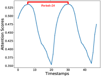
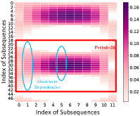
The local temporal correlation is constructed as an attention score between the Gaussian location $\mathbf{h}_{i}$ and each observation in a historical subsequence $\mathbf{M}_{i}$. In Figure 6(a), the x-axis denotes timestamps of 48 observations in subsequences, and the y-axis denotes the attention score between a Gaussian location and an observation at a timestamp. A higher attention score signifies a higher temporal importance of an observation to an Gaussian location and thus to the final prediction. The Gaussian process uses its covariance matrix to represent the global temporal correlations among subsequences, as illustrated in Figure 6(b), where darker colors indicate higher positive correlations and lighter colors indicate higher negative correlations. In addition, values in the covariance matrix represent the covariances of pairs of subsequences.

We observe that: both local and global temporal correlations are able to discover periodic patterns. The change of attention score in Figure 6(a) is consistent with the change of the observations in M4 Hourly-210, which exhibits a regular period of 24 timestamps (hours). Therefore, the attention module captures and constructs local temporal correlations. Further, each column in Figure 6(b) represents the covariance change between the current subsequence and other subsequences, which also matches the ground truth—the period is 24 hours. Next, we observe that the global temporal correlations capture different short term dependencies, that the local correlations fail to capture. As shown in the two oval shapes in Figure 6(b), the short-term dependencies of distinct subsequences are different. For example, the short-term dependencies of other subsequences to subsequence 1 and to subsequence 5 are distinct. The Attention module fails to capture such diversity because the attention parameters of learning Gaussian locations from input subsequences are shared. The Gaussian process compensates for this weakness of the Attention module by capturing the diversity among subsequences using global temporal correlations, thus improving the prediction accuracy.

5.3.2. Multivariate Correlations

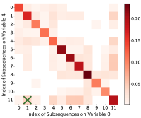
AutoGP utilizes a multivariate covariance matrix to capture the correlations between each two subsequences of two variables. An example matrix that captures the correlation between variables 0 and 4 is shown in Figure 6(c), where darker colors indicate higher positive correlations and lighter colors indicate higher negative correlations. We observe that the correlations between different subsequences of different variables can be captured. For example, subsequence 1 of variable 0 has a high positive correlation with subsequence 11 of variable 4, as indicated by the cross in Figure 6(c).

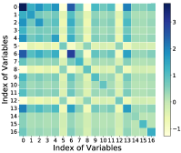
We show cross-variable weights in Figure 6(d). The higher an absolute weight value is, the higher the importance of the corresponding variable. By selecting variables with high correlations and discarding variables with low correlations during prediction, AutoGP captures important information and reduces the risk of overfitting.

In order to demonstrate the importance of correlated variables to the forecasting accuracy, we use IMV-LSTM and TFT as baselines to evaluate the effectiveness of feature selection. We select the variables with the top 50% correlations for AutoGP, IMV-LSTM, and TFT. Furthermore, to verify that the correlated variables affect the target variable, we include an additional baseline—AutoGP-P, which selects the variable with the highest correlation to the target variable. The results with standard errors in Table 5 show that AutoGP achieves the highest prediction accuracy in most cases. Removing uncorrelated variables decreases the risk of overfitting. In addition, the training time for each epoch decreases to $7.44\%$ of the original one, as the amount of data is decreased.

5.4. Ablation Study

5.4.1. Study of AutoGP

The results of the ablation study of AutoGP are shown in Table 6, where w/o Att, w/o CVW, and w/o KAS denote AutoGP without the attention structure, cross-variable weights, and KAS, respectively. In addition, AutoGP-G replaces KAS with greedy kernel search.

First, w/o Att replaces AutoGP’s attention structure with a fully connected neural network. As a result, the model misses temporal correlations within subsequences, and the prediction accuracy decreases slightly.

Next, w/o Pa-att replaces AutoGP’s patch-attention with a self-attention structure, thus offering information on the advantages of patch-attention over self-attention when processing time series. The results show that patch-attention performs better for large horizons. It reduces the connections between attention structures to improve the ability of the model to capture key features in long subsequences.

Third, w/o CVM performs poorly on SML2010, but performs well on Electricity. This is because of the variables of SML2010 record different aspects, such as indoor temperature, carbon dioxide concentration, and light intensity. In contrast, the variables of Electricity record similar data—the power consumption of different users. Without cross-variable weights and using only a shared kernel function, AutoGP is incapable of capturing the diverse multivariate correlations among subsequences in SML2010, thus reducing the prediction accuracy. The time series in Electricity record the same type of data, so the effect of cross-variable weights is not obvious.

Fourth, we observe that w/o KAS performs well on SML2010 and poorly on Electricity, as the seasonality and short-term dependency patterns in SML2010 are simple. In contrast, the patterns in Electricity are complex, including combinations of, e.g., long-term dependencies and hybrids of short-term dependencies and seasonality. We use a spectral mixture kernel as the prior for w/o KAS, which works well for the time series in SML2010. However, this simple prior is incapable of capturing the complex correlations in Electricity.

Finally, AutoGP-G and AutoGP achieve similar prediction accuracy on multivariate datasets because they are both able to discover complex kernel functions.

Table 8. Demonstration of Final Kernel

Search Method	Time Series Pattern
KAS	SE+PER+SE$\times$PER+PER2+SE2
Greedy	SE+PER+SE$\times$PER+PER2+LIN+RQ+(SE+RQ)+(PER+SE)

5.4.2. Study of KAS

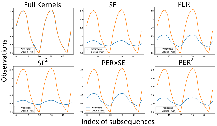
The kernels obtained by KAS and greedy kernel search may be different. As greedy kernel search is a greedy method and the input order of kernels is random, it tends to return locally optimal results. Hourly-210 is a time series in M4 that contains 1,008 observations with only periodic and short-term patterns. In the first iteration, with parameter initialization, the validation loss will be reduced with a high probability. Therefore, if the randomly input kernel in the first iteration is a LIN kernel, the greedy kernel search will preserve the LIN kernel, representing a linear pattern with a high probability. The greedy kernel search introduced redundant patterns into the model, thus causing overfitting of the model and decreasing prediction accuracy. In contrast, KAS searches all kernel functions at the training stage without random input, so it does not fall into the local optimum. To evaluate whether KAS can overcome overfitting, we utilize all four base kernel functions, and Table 8 shows the final kernel functions obtained by KAS and greedy kernel search when $R=2$ on Hourly-210. The domain of kernel functions is closed under addition, so the pattern found by KAS can be disassembled into multiple independent simple patterns. As shown in Figure 7, each kernel captures part of the information of the whole time series. Each pattern has its own analytic form, shown in Table 1. The blue pattern in Table 8 denotes a kernel found by KAS, but not by the greedy method, and the red patterns are kernels found by the greedy method, but not by KAS.

Figure 7. Visualization of Decomposed Kernels

The results are shown in Table 7, where KAS-Full and Greedy-Full denote the kernels learned via KAS and greedy kernel search, w/o means that we remove one kernel from KAS-Full, and w/ means that we add one kernel to KAS-Full that is discovered by Greedy-Full but not by KAS-Full. When we remove any kernel from KAS-Full, the prediction accuracy of AutoGP decreases because the missing pattern causes the model to underfit. Further, when we add a kernel, the prediction accuracy also decreases, as inclusion of the additional pattern leads to overfitting. Specifically, the result ”w/LIN” proves that the LIN kernel decreases the prediction accuracy, which, however, is contained in the kernel set searched by greedy kernel search.

(a) MAE

(b) Training Time

Figure 8. KAS vs. Greedy on M4 Hourly-210

(a) Training Time per Epoch

(b) Memory Usage

(c) MAE

Figure 9. Training Time and Scalability

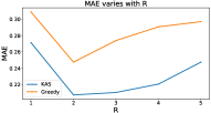
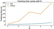
To assess the sensitivity to the depth of the kernel association $R$, we vary $R$. Figure 8(a) shows AutoGP and AutoGP-G generally achieve their highest prediction accuracy when $R=2$ or $R=3$. Although a larger $R$ results in the availability of more high-order hybrid patterns to fit the training data, this also increases the risk of overfitting. Finally, we report the training time of KAS and greedy kernel search. Figure 8(b) shows that KAS has a much lower running time than greedy search. Thus, we use $R=2$ for AutoGP and AutoGP-G in all experiments.

5.5. Training Time and Scalability

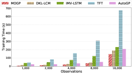
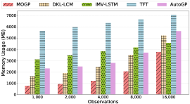
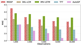
To evaluate the training time and memory usage of AutoGP, we design experiments on the sizeable multivariate dataset Electricity, which contains 370 variables. Each time series for one variable contains 26,304 observations, and the historical and forecasting horizons are set to 24. To ensure fairness of the results, we report the training time per epoch of each model. To assess the scalability of AutoGP, we report on experiments, where we use from 1000 to 16000 subsequences to train AutoGP. The sizes of the validation and test sets remain 10% and 20% of 26,304. We use a fixed kernel searched by KAS in advance for AutoGP to test the real training time.

We observe that the training times in Figure 9(a) and memory usage Figure 9(b) of the neural network-based methods IMV-LSTM and TFT are larger than those of the Gaussian-based methods MOGP, DKL-LCM, and AutoGP. However, the growth rates of the training times and memory usage of the Gaussian-based methods are larger than those of the neural network-based methods, as the Gaussian-based methods construct correlations between any two observations. Fortunately, we do not have to build the covariance matrix for all observations. As Figure 9(c) shows, the MAE decreases slightly when the number of observations exceeds 8,000 because when there are enough observations, the rate of decrease of MAE is slower.

6. Related Work

Time Series Forecasting with Correlation Learning: Time series forecasting methods utilize feature importance or temporal dynamics to explicitly learn correlations. Feature importance enables the learning of which variables or periods contribute the most to forecasting, by using attention-based methods (guo2019exploring, ; lim2021temporal, ; ismail2020benchmarking, ) that learn the importance of variables to other variables at each timestamp from attention scores, which are local correlations. Temporal dynamics concern the fluctuations or patterns of how the data changes over time, possibly described using characteristics such as frequency, trend, and seasonality. Wang et al. (wang2018multilevel, ) propose a multi-wavelet decomposition network that decomposes a time series into wavelets with different frequencies. Oreshkin et al. (oreshkin2019n, ) take advantage of residual calculation to enable pattern learning. Their modeling approach is capable of showing trend and seasonality by leveraging Holt-Winters inductive bias (holt2004forecasting, ). The above methods consider either feature importance or basic patterns of local correlations on univariate time series. In contrast, our proposal targets complex patterns and global correlations among multiple time series.

Gaussian Process: The applications of Gaussian processes in neural networks are divided into two areas—deep Gaussian process and deep kernel learning. Deep Gaussian processes (jankowiak2020deep, ; salimbeni2017doubly, ; damianou2013deep, ) replace each layer of the neural network with a Gaussian process to overcome overfitting. However, it is difficult to study correlations of time series explicitly with these methods. Next, deep kernel learning combines the structural properties of deep architectures with the non-parametric flexibility of kernel methods. Wilson et al. (wilson2016deep, ; wilson2016stochastic, ) combine a neural network and a Gaussian process layer with a spectral mixture kernel. Al-Shedivat et al. (al2017learning, ) propose to learn kernels with LSTMs so that the kernels encapsulate the properties of LSTMs. However, these methods lack the ability to model the diversity exhibited in multivariate time series. To achieve that, we propose a deep kernel model that combines the advantage of kernels, which model naturally the dynamics of time series, and the advantage of deep learning, which is able to learn complex parameters in kernels and covariance matrices. In addition, to capture the multivariate covariance among time series, multi-task Gaussian process models (bonilla2007multi, ; wilson2011gaussian, ; titsias2011spike, ; guarnizo2015indian, ) utilize fixed and pre-defined kernel functions, which limit their capability of capturing diverse correlations. Linear coregionalization models (alvarez2008sparse, ; alvarez2012kernels, ; ulrich2015gp, ; parra2017spectral, ; tong2019discovering, ) use linear combinations of kernel functions to enhance model adaptability. However, these proposals assume a purely Gaussian process framework and are difficult to transfer to deep architectures and to adapt to enable autoregressive time series forecasting.

Kernel Learning: Kernel methods are used in two main areas of machine learning—support vector machines (SVM) and Gaussian processes. SVM-based kernel learning methods (paparrizos2019grail, ; chang2011libsvm, ) are utilized for time series classification, and Gaussian process-based kernel learning methods are used for time series forecasting. Gaussian process-based methods generate new kernels by combining existing kernels (schulz2017compositional, ) via kernel association. A selection strategy determines how to select the best kernels, using, e.g., greedy search (duvenaud2013structure, ; kim2018scaling, ; lu2018structured, ; schulz2016probing, ; schulz2017compositional, ; tong2019discovering, ). However, existing kernels learning approaches suffer from high time complexity. These methods utilize the Bayesian information criterion to select optimal kernel functions. Sun et al. (sun2018differentiable, ) propose a neural network that alternates stacked linear and interactive layers to simulate kernel association. However, the capacity of the kernel function space is fixed, which may lead to sub-optimal kernels. We propose a dynamic and efficient kernel learning framework that is integrated well into a deep architecture.

7. Conclusion and future work

We propose an autoregressive Gaussian process modeling framework that enables the learning of multivariate time series forecasting models. The framework captures local and global temporal and multivariate correlations with the goal of improving forecasting accuracy. In addition, we propose KAS, a novel kernel search method that enables the framework to capture complex and diverse temporal correlations. Finally, the framework includes means of capturing cross-variable weights, which enable models that capture distinct multivariate correlations. Extensive experiments show that AutoGP is capable of better prediction accuracy than its competitors. And AutoGP provides visualized temporal and multivariate correlations. In future work, it is of interest to extend the proposed framework to cover outlier detection (kieu2022robust, ) and neural network interpretability (zhang2021survey, ).

References

- [1] Jingyuan Wang, Ze Wang, Jianfeng Li, and Junjie Wu. Multilevel wavelet decomposition network for interpretable time series analysis. In Proceedings of the 24th ACM SIGKDD International Conference on Knowledge Discovery & Data Mining, pages 2437–2446, 2018.
- [2] Lei Bai, Lina Yao, Salil S Kanhere, Zheng Yang, Jing Chu, and Xianzhi Wang. Passenger demand forecasting with multi-task convolutional recurrent neural networks. In Pacific-Asia Conference on Knowledge Discovery and Data Mining, pages 29–42. Springer, 2019.
- [3] Zonghan Wu, Shirui Pan, Guodong Long, Jing Jiang, and Chengqi Zhang. Graph wavenet for deep spatial-temporal graph modeling. arXiv preprint arXiv:1906.00121, 2019.
- [4] David Campos, Tung Kieu, Chenjuan Guo, Feiteng Huang, Kai Zheng, Bin Yang, and Christian S Jensen. Unsupervised time series outlier detection with diversity-driven convolutional ensembles–extended version. arXiv preprint arXiv:2111.11108, 2021.
- [5] Bryan Lim, Sercan Ö Arık, Nicolas Loeff, and Tomas Pfister. Temporal fusion transformers for interpretable multi-horizon time series forecasting. International Journal of Forecasting, 37(4):1748–1764, 2021.
- [6] Haixu Wu, Jiehui Xu, Jianmin Wang, and Mingsheng Long. Autoformer: Decomposition transformers with auto-correlation for long-term series forecasting. Advances in Neural Information Processing Systems, 34:22419–22430, 2021.
- [7] Haoyi Zhou, Shanghang Zhang, Jieqi Peng, Shuai Zhang, Jianxin Li, Hui Xiong, and Wancai Zhang. Informer: Beyond efficient transformer for long sequence time-series forecasting. In Proceedings of AAAI, pages 11106–11115, 2021.
- [8] Boris N Oreshkin, Dmitri Carpov, Nicolas Chapados, and Yoshua Bengio. N-beats: Neural basis expansion analysis for interpretable time series forecasting. arXiv preprint arXiv:1905.10437, 2019.
- [9] Lei Bai, Lina Yao, Can Li, Xianzhi Wang, and Can Wang. Adaptive graph convolutional recurrent network for traffic forecasting. Advances in neural information processing systems, 33:17804–17815, 2020.
- [10] Razvan Gabriel Cirstea, Tung Kieu, Chenjuan Guo, Bin Yang, and Sinno Jialin Pan. Enhancenet: Plugin neural networks for enhancing correlated time series forecasting. In 37th IEEE International Conference on Data Engineering, ICDE 2021, pages 1739–1750. IEEE, 2021.
- [11] David Hallac, Youngsuk Park, Stephen Boyd, and Jure Leskovec. Network inference via the time-varying graphical lasso. In Proceedings of the 23rd ACM SIGKDD International Conference on Knowledge Discovery and Data Mining, pages 205–213, 2017.
- [12] Defu Cao, Yujing Wang, Juanyong Duan, Ce Zhang, Xia Zhu, Congrui Huang, Yunhai Tong, Bixiong Xu, Jing Bai, Jie Tong, et al. Spectral temporal graph neural network for multivariate time-series forecasting. Advances in neural information processing systems, 33:17766–17778, 2020.
- [13] Ashish Vaswani, Noam Shazeer, Niki Parmar, Jakob Uszkoreit, Llion Jones, Aidan N Gomez, Łukasz Kaiser, and Illia Polosukhin. Attention is all you need. In Proceedings of the 31st International Conference on Neural Information Processing Systems, pages 6000–6010, 2017.
- [14] Razvan-Gabriel Cirstea, Chenjuan Guo, Bin Yang, Tung Kieu, Xuanyi Dong, and Shirui Pan. Triformer: Triangular, variable-specific attentions for long sequence multivariate time series forecasting. In Proceedings of the Thirty-First International Joint Conference on Artificial Intelligence, pages 1994–2001, 2022.
- [15] Andrew Wilson and Ryan Adams. Gaussian process kernels for pattern discovery and extrapolation. In International conference on machine learning, pages 1067–1075. PMLR, 2013.
- [16] Anh Tong and Jaesik Choi. Discovering latent covariance structures for multiple time series. In International Conference on Machine Learning, pages 6285–6294. PMLR, 2019.
- [17] Christopher K Williams and Carl Edward Rasmussen. Gaussian processes for machine learning. MIT press Cambridge, MA, USA, 2006.
- [18] Andrew Gordon Wilson. Covariance kernels for fast automatic pattern discovery and extrapolation with Gaussian processes. PhD thesis, University of Cambridge Cambridge, UK, 2014.
- [19] Carl Edward Rasmussen. Gaussian processes in machine learning. In Summer school on machine learning, pages 63–71. Springer, 2003.
- [20] Maruan Al-Shedivat, Andrew Gordon Wilson, Yunus Saatchi, Zhiting Hu, and Eric P Xing. Learning scalable deep kernels with recurrent structure. The Journal of Machine Learning Research, 18(1):2850–2886, 2017.
- [21] David Duvenaud, James Lloyd, Roger Grosse, Joshua Tenenbaum, and Ghahramani Zoubin. Structure discovery in nonparametric regression through compositional kernel search. In International Conference on Machine Learning, pages 1166–1174. PMLR, 2013.
- [22] Yuichi Motai. Kernel association for classification and prediction: A survey. IEEE transactions on neural networks and learning systems, 26(2):208–223, 2014.
- [23] Trevor Hastie, Robert Tibshirani, Jerome H Friedman, and Jerome H Friedman. The elements of statistical learning: data mining, inference, and prediction, volume 2. Springer, 2009.
- [24] Roger Grosse, Ruslan R Salakhutdinov, William T Freeman, and Joshua B Tenenbaum. Exploiting compositionality to explore a large space of model structures. arXiv preprint arXiv:1210.4856, 2012.
- [25] James Robert Lloyd, David Duvenaud, Roger Grosse, Joshua B Tenenbaum, and Zoubin Ghahramani. Automatic construction and natural-language description of nonparametric regression models. stat, 1050:24, 2014.
- [26] Hanxiao Liu, Karen Simonyan, and Yiming Yang. Darts: Differentiable architecture search. arXiv preprint arXiv:1806.09055, 2018.
- [27] Xinle Wu, Dalin Zhang, Chenjuan Guo, Chaoyang He, Bin Yang, and Christian S Jensen. Autocts: Automated correlated time series forecasting. Proceedings of the VLDB Endowment, 15(4):971–983, 2021.
- [28] Gabriel Parra and Felipe Tobar. Spectral mixture kernels for multi-output gaussian processes. In Proceedings of the 31st International Conference on Neural Information Processing Systems, pages 6684–6693, 2017.
- [29] Andrew Gordon Wilson, Zhiting Hu, Ruslan Salakhutdinov, and Eric P Xing. Stochastic variational deep kernel learning. Advances in Neural Information Processing Systems, pages 2594–2602, 2016.
- [30] Andrew Gordon Wilson, Zhiting Hu, Ruslan Salakhutdinov, and Eric P Xing. Deep kernel learning. In Artificial intelligence and statistics, pages 370–378. PMLR, 2016.
- [31] Spyros Makridakis, Evangelos Spiliotis, and Vassilios Assimakopoulos. The m4 competition: Results, findings, conclusion and way forward. International Journal of Forecasting, 34(4):802–808, 2018.
- [32] Hoang Anh Dau, Anthony Bagnall, Kaveh Kamgar, Chin-Chia Michael Yeh, Yan Zhu, Shaghayegh Gharghabi, Chotirat Ann Ratanamahatana, and Eamonn Keogh. The ucr time series archive. IEEE/CAA Journal of Automatica Sinica, 6(6):1293–1305, 2019.
- [33] Fransisco Zamora-Martinez, Pablo Romeu, Pablo Botella-Rocamora, and Juan Pardo. On-line learning of indoor temperature forecasting models towards energy efficiency. Energy and Buildings, 83:162–172, 2014.
- [34] Yaguang Li, Rose Yu, Cyrus Shahabi, and Yan Liu. Diffusion convolutional recurrent neural network: Data-driven traffic forecasting. arXiv preprint arXiv:1707.01926, 2017.
- [35] Tian Guo, Tao Lin, and Nino Antulov-Fantulin. Exploring interpretable lstm neural networks over multi-variable data. In International conference on machine learning, pages 2494–2504. PMLR, 2019.
- [36] Diederik P Kingma. &ba j.(2014). adam: A method for stochastic optimization. arXiv preprint arXiv:1412.6980, 2015.
- [37] Fabrício José Pontes, GF Amorim, Pedro Paulo Balestrassi, AP Paiva, and João Roberto Ferreira. Design of experiments and focused grid search for neural network parameter optimization. Neurocomputing, 186:22–34, 2016.
- [38] Aya Abdelsalam Ismail, Mohamed Gunady, Héctor Corrada Bravo, and Soheil Feizi. Benchmarking deep learning interpretability in time series predictions. In Proceedings of the 34th International Conference on Neural Information Processing Systems, pages 6441–6452, 2020.
- [39] Charles C Holt. Forecasting seasonals and trends by exponentially weighted moving averages. International journal of forecasting, 20(1):5–10, 2004.
- [40] Martin Jankowiak, Geoff Pleiss, and Jacob Gardner. Deep sigma point processes. In Conference on Uncertainty in Artificial Intelligence, pages 789–798. PMLR, 2020.
- [41] Hugh Salimbeni and Marc Peter Deisenroth. Doubly stochastic variational inference for deep gaussian processes. In Proceedings of the 31st International Conference on Neural Information Processing Systems, pages 4591–4602, 2017.
- [42] Andreas Damianou and Neil D Lawrence. Deep gaussian processes. In Artificial intelligence and statistics, pages 207–215. PMLR, 2013.
- [43] Edwin V Bonilla, Kian Ming A Chai, and Christopher KI Williams. Multi-task gaussian process prediction. In Proceedings of the 20th International Conference on Neural Information Processing Systems, pages 153–160, 2007.
- [44] Andrew Gordon Wilson, David A Knowles, and Zoubin Ghahramani. Gaussian process regression networks. arXiv preprint arXiv:1110.4411, 2011.
- [45] Michalis K Titsias and Miguel Lázaro-Gredilla. Spike and slab variational inference for multi-task and multiple kernel learning. In Proceedings of the 24th International Conference on Neural Information Processing Systems, pages 2339–2347, 2011.
- [46] Cristian Guarnizo, Mauricio A Álvarez, and Alvaro A Orozco. Indian buffet process for model selection in latent force models. In Iberoamerican Congress on Pattern Recognition, pages 635–642. Springer, 2015.
- [47] Mauricio Alvarez and Neil D Lawrence. Sparse convolved gaussian processes for multi-output regression. In Proceedings of the 21st International Conference on Neural Information Processing Systems, pages 57–64, 2008.
- [48] Mauricio A Alvarez, Lorenzo Rosasco, Neil D Lawrence, et al. Kernels for vector-valued functions: A review. Foundations and Trends® in Machine Learning, 4(3):195–266, 2012.
- [49] Kyle Ulrich, David E Carlson, Kafui Dzirasa, and Lawrence Carin. Gp kernels for cross-spectrum analysis. In Proceedings of the 28th International Conference on Neural Information Processing Systems-Volume 2, pages 1999–2007, 2015.
- [50] John Paparrizos and Michael J Franklin. Grail: efficient time-series representation learning. Proceedings of the VLDB Endowment, 12(11):1762–1777, 2019.
- [51] Chih-Chung Chang. Libsvm: a library for support vector machines, acm transactions on intelligent systems and technology, 2: 27: 1–27: 27, 2011. http://www. csie. ntu. edu. tw/~ cjlin/libsvm, 2, 2011.
- [52] Eric Schulz, Joshua B Tenenbaum, David Duvenaud, Maarten Speekenbrink, and Samuel J Gershman. Compositional inductive biases in function learning. Cognitive psychology, 99:44–79, 2017.
- [53] Hyunjik Kim and Yee Whye Teh. Scaling up the automatic statistician: Scalable structure discovery using gaussian processes. In International Conference on Artificial Intelligence and Statistics, pages 575–584. PMLR, 2018.
- [54] Xiaoyu Lu, Javier Gonzalez, Zhenwen Dai, and Neil D Lawrence. Structured variationally auto-encoded optimization. In International conference on machine learning, pages 3267–3275. PMLR, 2018.
- [55] Eric Schulz, Joshua B Tenenbaum, David Duvenaud, Maarten Speekenbrink, and Samuel J Gershman. Probing the compositionality of intuitive functions. In Proceedings of the 30th International Conference on Neural Information Processing Systems, pages 3736–3744, 2016.
- [56] Shengyang Sun, Guodong Zhang, Chaoqi Wang, Wenyuan Zeng, Jiaman Li, and Roger Grosse. Differentiable compositional kernel learning for gaussian processes. In International Conference on Machine Learning, pages 4828–4837. PMLR, 2018.
- [57] Tung Kieu, Bin Yang, Chenjuan Guo, Christian S Jensen, Yan Zhao, Feiteng Huang, and Kai Zheng. Robust and explainable autoencoders for unsupervised time series outlier detection. In Proceeding of the 38th IEEE International Conference on Data Engineering, ICDE 2022, pages 3038–3050, 2022.
- [58] Yu Zhang, Peter Tiňo, Aleš Leonardis, and Ke Tang. A survey on neural network interpretability. IEEE Transactions on Emerging Topics in Computational Intelligence, pages 726–742, 2021.